

Submitted:
01 September 2026
Posted:
02 September 2026
You are already at the latest version
Abstract
The range of local sequence–structure correlation is known for coarse-grained descriptors — secondary structure and side-chain burial — but not for the backbone dihedrals themselves. I measure the information local sequence carries about φ and ψ at 10° resolution against how far a translation-equivariant convolutional model may look. Both peak at a window radius of 8 residues — φ recovering 0.330 bits of its 3.669 and ψ 0.429 of its 4.161 on held-out chains — and decline beyond. Controls test the alternatives: rebinning at 5°, 20° and 30° leaves the radius at 8, profiles do not widen it, and capacity does not rescue a wider one — every radius-32 model tried, to 556,324 weights, scores below every radius-8 model. A parameter-free mutual-information estimate finds the signal at the null level by |d| ≈ 10 downstream, ≈ 8 upstream. On a second dataset of 8,589 chains, no 30% cluster shared across splits, both maxima again fall at 8, though ψ is flat to 16.Decomposed by class, coil carries three times what helix does beyond its own marginal (0.376 against 0.120 bits), though all three retain about 90% of what they fit. An earlier version reported that helix retains none; that is withdrawn. It came of scoring a small split against a class marginal fitted on that same split — an oracle whose advantage equals the train-to-split entropy gap, here 0.369 bits, larger than the helix signal. I report three evaluation errors able to invert conclusions; that is the third.
Keywords:
protein conformation
; protein structure
; secondary
; amino acid sequence
; information theory
; computational biology
; neural networks
Introduction
That an amino acid sequence determines its structure is not in dispute. How much of that determination is expressible locally — as a function of a bounded window of neighbouring residue identities — is a separate and quantitative question, and it bears directly on what any single-sequence predictor can achieve.
Crooks and Brenner addressed this for secondary structure, finding that only about one quarter of the information required to specify it is available from local inter-sequence correlations, and that the important interactions are short ranged.¹ A companion study extended the measurement across amino acid identity, three-state secondary structure and four-state side-chain burial, reporting a total sequence–structure information content of roughly 0.35 bits per residue and a correlation profile that decays over a few residues.² Both studies reduce conformation to a coarse-grained descriptor: each residue is represented by one β-carbon coordinate, and secondary structure enters as a three-state proxy for the backbone torsions rather than as the torsions themselves.
The backbone torsions have been the natural coordinates for local conformation since Ramachandran and colleagues mapped their sterically allowed combinations.³ They have been measured against sequence directly, but at short range. Solis quantified the mutual information between sequence and Ramachandran φ/ψ using an information-maximisation partition, reporting up to 0.417 nats for a tripeptide — a central residue and its two immediate flanks.⁴˒⁵ The analysis does not extend beyond ±1 residue, so it cannot say where the signal ends.
Networks that predict the dihedrals from sequence are now numerous and accurate. Current methods reach mean absolute errors of roughly 15–20° for φ using deep architectures over evolutionary profiles and predicted contact maps,⁶ with comparable single-sequence predictors for cases where no alignment is available.⁷ Their aim is accuracy rather than measurement: the input window is a design parameter tuned for performance, not a quantity swept to locate where the signal ends, and none reports the reach of what it exploits. The closest in intent is the older network of Helles and Fonseca, who trained one on an input window of seven residues to emit a probability distribution over 30° × 30° cells of Ramachandran space for the window’s central residue, restricted to coil segments.8 The output is of the same kind as the one used here, but the window is a fixed ±3 chosen as a design parameter rather than a quantity swept, and the aim is prediction accuracy rather than measurement. Škrbić and colleagues later examined local sequence–structure relationships across more than 4,000 structures and found the correlation weak against a random assignment of sequence to structure;9 their local descriptor is a pair of Cα-based angles rather than the backbone torsions themselves, and they report no dependence on sequence separation.
This leaves a specific gap. The published separation profiles for secondary structure and burial extend to ±8 residues;² the published dihedral measurement extends to ±1,⁴ and the widest window used by a dihedral predictor of this kind to ±3.8 No measurement locates the point at which additional sequence context stops contributing to a backbone torsion, and none reports whether that point is the same for φ and for ψ.
I close that gap with a model whose receptive field is an explicit, swept parameter, and corroborate it with a parameter-free counting estimate. I then decompose the result by secondary structure class. Here the qualitative direction is not new: Swindells, MacArthur and Thornton derived intrinsic φ/ψ propensities specifically from coil regions, because helix and strand residues confound intrinsic backbone preference with secondary-structure stabilisation, and the coil-library approach built on that observation is standard.10 What has not been reported is the size of the effect in bits, measured on a held-out split large enough to carry the decomposition. Doing so also exposes a hazard in how such decompositions are scored, which is reported alongside the measurement.
Materials and Methods
Data
All structures analysed are public depositions in the Protein Data Bank.11 They were taken from three non-overlapping sets: a training set of 3,276 chains, a validation set of 177 chains used for early stopping and model selection, and a held-out test set of 65 chains scored once per configuration. Backbone dihedrals were computed from deposited coordinates and secondary structure taken from the HELIX and SHEET records of the deposition, reduced to three classes (helix, strand, coil). The assignment is therefore the depositors’ rather than one recomputed from coordinates by a single algorithm.12 Splits are assigned deterministically by a hash of the chain identifier, so they are reproducible and independent of file ordering.
A second, independent dataset was built for the replication reported below. Its chains come from a PISCES13 `cullpdb` list at 25% sequence identity, resolution 2.0 Å or better, R ≤ 0.25, X-ray only — 8,589 chains and 2,143,481 residues against the first set’s 3,518 and 619,746. Two differences from the original construction are deliberate. Splits are assigned by hashing the connected component of entries linked by a shared RCSB 30% sequence cluster rather than the chain, so no such cluster can cross a split boundary; assigning chains independently leaves 180 clusters straddling, because those clusters are transitive and a 25% pairwise cut does not prevent it. And the set is X-ray only, where the original includes NMR ensembles, whose dihedrals are a different measurement. The proportions are 80/10/10, giving 818 test chains and 206,774 scored φ values in place of 65 and 16,715. Because the training marginal differs, so does H₀: for φ, 2.4653 nats on validation and 2.4695 on test; for ψ, 2.8262 and 2.8316. Bits measured on one dataset are therefore not comparable to bits measured on the other, and only the location of the maximum is.
Angles were discretised into 36 bins of 10°. The partition is stated here because every quantity in this paper is measured over it: an angle is wrapped into [0°, 360°) and assigned to bin k = ⌊θ/10°⌋, so bin edges fall at multiples of 10° from 0° and no bin is centred on 0° or ±180°. A bin’s representative angle, used wherever a result is quoted in degrees, is its centre, reported in (−180°, 180°]. φ is undefined at the N-terminal residue and ψ at the C-terminal residue; those positions are excluded from training and from scoring, and are not counted in any reported n.
All reported information is the reduction in cross-entropy against the training-set marginal for that torsion, evaluated on the scored split and converted to bits as (H₀ − NLL) / ln 2, where H₀ is the cross-entropy of the training marginal on the split being scored. This makes every figure a statement about information gained relative to a predictor that uses no sequence at all. For φ, H₀ = 2.5708 nats on validation and 2.5434 on test; for ψ, 2.9455 and 2.8844. The corresponding total entropies are 3.709 and 3.669 bits for φ, 4.249 and 4.161 for ψ.
I report information rather than accuracy deliberately. Tolerance-based accuracy is dominated by how concentrated the answer already is: helix φ barely varies, so a constant achieves a high score there without using any sequence.
The validation split does two jobs — early stopping selects the epoch on it, and the per-class breakdown is reported on it because the 65-chain test split is too small for that decomposition — so for the per-class breakdown it is divided into disjoint halves. Chains are sorted by name and taken alternately, giving 89 chains for selection and 88 for reporting; the epoch is chosen on one half and the figures quoted from the other. Alternating rather than splitting front-to-back matters, because a name-sorted list is not random with respect to deposition era or structural family.
Because the 10° discretisation is a choice, the radius sweep was repeated at 5° (72 bins), 20° (18 bins) and 30° (12 bins). The 20° and 30° datasets are exact coarsenings of the 10° one — two or three bins merged into one, so no angle moves and the chains are identical. The 5° dataset was re-prepared from the original coordinates and reproduces the same 3,276 / 177 / 65 chains and 558,905 / 44,126 / 16,715 residues. Bits are not comparable across resolutions, since a finer target is harder to hit, and each resolution is therefore scored against its own H₀, computed from the training marginal at that bin width; the location of the peak is comparable, and that is what the control tests.
Model
The model is a stack of one-dimensional convolutions over the residue-type one-hot encoding, 21 channels: the twenty amino acids and one slot into which anything else — a modified or unresolved residue — falls. Weights are indexed by input residue type, sequence separation and layer — never by absolute position — so a motif learned at one point in a chain is recognised at every other, and the model runs on chains of any length. This is a translation-equivariant weight-sharing scheme equivalent to a relative-position bias. At the reported configuration — radius 8, 64 units, four pointwise hidden layers — this is a model with 37,732 weights, small enough that its capacity is worth testing rather than assuming, and the Results do so.
For the radius sweep, the layers above the first are pointwise (kernel width 1). The total receptive radius of the stack is therefore exactly the first-layer radius and nothing else; without this constraint each hidden layer would silently contribute its own reach and the swept axis would not mean what it says. Depth (4 hidden layers), width (64 units), objective, learning rate and stopping rule are held fixed across the sweep, so the only quantity varying is how far along the chain the model may look.
The output is a softmax over the 36 bins, trained by cross-entropy against a von Mises target14 centred on the true bin with an angular width of 10° — label smoothing that respects the periodicity of the variable. The target is the von Mises density with κ = 1/σ², σ = 10° in radians, evaluated at the bin centres using the shortest circular distance between bins, then normalised over the 36. Here σ is a Gaussian-equivalent angular width — the small-angle limit in which a von Mises approaches a wrapped normal — rather than the von Mises circular standard deviation as formally defined; the quantity actually used is the concentration κ = 32.8. The width is deliberately one bin, since it encodes only that adjacent bins are nearly the same angle. Genuine conformational spread is meant to emerge from disagreement between training examples rather than be written into the target. A distribution, rather than a point estimate, is the appropriate answer for a position whose torsion genuinely varies.
The 36 outputs are therefore competing scores over one softmax, not 36 independent bits: an angle is never represented as a binary pattern anywhere in the model, and the training target for a residue is a real-valued vector over the bins summing to one (0.397 at the true bin, 0.241 either side, falling to 0.005 three bins out). The only one-hot in the model is the residue-type input. I note this because the released code also contains a bitwise thermometer coding of the angle, in which Hamming distance equals circular distance; it is the scheme the predecessor codebase used, regenerated rather than transcribed and retained so that its results remain reproducible, and it is not used for anything reported here.
Where a single predicted bin is needed — for accuracy against a tolerance, and for mean angular error — it is the argmax of the predicted distribution, and the corresponding angle is that bin’s centre. Every information figure, by contrast, uses the full predicted distribution and never the point estimate.
Training uses Adam with global gradient-norm clipping, mini-batches of 16 chains, early stopping on validation negative log likelihood with patience 10 and an epoch cap of 60. The one exception is the evolutionary-profile control of the Discussion, which uses patience 25 and a cap of 200 because the profile input converges much more slowly at narrow radii; it is described there as an extended-convergence run and its own control arm is trained under the same allowance. The activation is the logistic sigmoid. Across three seeds it outperformed ReLU by 0.036 bits on the test split and tanh by 0.026, and its worst seed beat every ReLU and tanh seed on both splits, by acting as a constraint on overfitting rather than as a smaller effective step.
Model-Free Estimate
To separate what is present from what one architecture can reach, I also estimated the pairwise mutual information between the residue type at separation d and the φ bin at position i, over 542,144 training residues, with no model. That count is smaller than the 558,905 residues in the training split because φ is undefined at the N-terminal residue of every chain and at every chain break; no residue is lost to the 21st input channel, since no residue carrying a non-standard type has a defined φ in this dataset.
Two corrections are essential. First, a plug-in mutual information is biased upward; with 20 residue types and 36 bins there are 720 cells, and even independent data fills them unevenly. At this sample size that bias is of order 0.001 bits — the same magnitude as the quantity being sought at large d — so the floor is measured by permutation rather than assumed, and subtracted: every value reported is the raw plug-in estimate minus the mean of twenty permutation replicates, and it is that difference the figure plots.
Second, the permutation null must be computed within each chain. A global permutation preserves both marginals but destroys something real: chains differ in secondary-structure content, so a helix-rich chain has both more of certain residue types and more helical φ. Under a global null that composition effect scores as signal. In these data it produced a flat pedestal of 0.0009 bits that did not decay out to d = 40, which reads as long-range coupling and is nothing of the kind. Permuting each chain’s angles among its own positions leaves composition intact and removes only the position-specific association; the pedestal disappears. This is consistent with the observation that neighbouring amino acids are themselves almost uncorrelated,² which means the pedestal could not have been local sequence autocorrelation.
Baselines
Where a tolerance-based score is used, the optimal constant baseline is the bin whose ±k window covers the most mass, not the modal bin. These coincide for a sharply peaked distribution and diverge for a broad one. φ in β-strand is the adverse case: in this training set the tallest single bin fell at helical φ (12.7% of strand-labelled residues, most likely mislabelled or frayed strand ends), and a modal-bin baseline built on it scored 5.9% on the test split — below the 8.3% chance level for a ±1-bin tolerance over 36 bins. The error runs one way only: an understated baseline flatters every model measured against it.
Redundancy
Sequence redundancy between the training and evaluation sets was assessed three ways of increasing stringency: a k-mer screen, Smith–Waterman15 alignment with a 60% coverage constraint, computed with parasail,16 and membership of the RCSB 30% sequence-identity clusters, which are computed independently of this work and are transitive. 32% of validation and 20% of test chains share a 30% cluster with training. Removing them moves validation from 0.332 to 0.330 bits and moves test in the opposite direction, from 0.329 to 0.332. The removed subsets score above the remainder on validation (0.338) and below it on test (0.314) — the signature of noise, not leakage. The alignment-based cull agrees: discarding every evaluation chain above 40% identity to any training chain leaves 0.330 bits on validation and 0.332 on test. I note that the correct remedy is to filter the evaluation set: training on redundant data is not an error, evaluating on data related to it is.
Availability
All source code, run scripts, analysis scripts and result files are released; see the Data Availability Statement. Every figure is regenerated from the released result files by a single script.
Results
Both Torsions Saturate at Radius 8
Figure 1 shows information recovered against window radius, for φ and ψ, on the held-out test split. Both curves rise steeply to radius 8 and decline beyond it. φ peaks at 0.330 bits and ψ at 0.429 (mean of three seeds, range 0.423–0.435); neither plateaus. Radius 32 — four times the reach and roughly four times the first-layer parameters — recovers less than radius 8 for both angles.
That the peak coincides for two different torsions is the central observation. ψ has more entropy to give up (4.161 bits against 3.669 on test) and yields more of it, both absolutely (0.429 against 0.330) and as a share of its own total (10.3% against 9.0%). The two angles differ in magnitude, in chemistry and in which neighbouring atoms define them, and they reach their maximum at the same distance — which is consistent with the range being a property of the underlying sequence–structure code rather than of either angle alone, though a shared limiting range could in principle arise for other reasons.
The ordering of magnitudes is chemically sensible. φ is the rotation about the N–Cα bond, and is strongly constrained by the local steric environment around that bond, including interactions involving the residue’s own side chain; a radius-0 model already recovers about half of φ’s eventual total. ψ is the rotation about the Cα–C′ bond and changes the orientation of the carbonyl group, which hydrogen-bonds to a neighbour, so more of what determines it lies in the surrounding residues — which is what a window model is positioned to capture.
Seed variation is small relative to the effect. The three-seed φ replication was run with the ReLU activation, which locates the same peak on both splits at a uniformly lower level (Supporting Information Figure S1); within any one configuration the spread across seeds is at most 0.013 bits, against a peak-to-radius-32 difference of 0.060 bits for φ and 0.094 for ψ.
The Peak does not Depend on the Angular Resolution
Table I repeats the sweep at four bin widths spanning a sixfold range, with the total entropy of φ on the test split running from 2.34 bits at 30° to 4.64 bits at 5°. The argmax is radius 8 at every resolution. The recovered fraction rises as bins get coarser — 6.8% at 5°, 9.0% at 10°, 12.7% at 20°, 15.2% at 30° — which is expected, because a narrower target is harder to hit. It should not be read as more information: across a resolution range in which the total varies by a factor of two, the absolute quantity recovered at radius 8 moves only between 0.313 and 0.355 bits. Coarsening the bins buys a larger share of a smaller total, not a better measurement. The location of the optimum does not move.
The Decline Past Radius 8 is Statistically Decisive
A wider first layer necessarily has more weights, so within the sweep alone reach and capacity are confounded: radius 32 could be failing to find a weak signal rather than finding none. Two results answer this. A protein-level bootstrap17 on the test split (65 chains, 20,000 paired resamples — chains, not residues, because residues within a chain are not independent draws) gives the values in Table II. The models are resampled together on each replicate, so the chain-to-chain variation they share cancels in a difference. A dilated-kernel control, which increases reach at a fixed parameter count, points the same way: within that control reach helps out to 14 and costs 0.009 bits beyond it, and its widest configuration — reach 62 for the parameters of a five-layer stack — sits 0.026 bits below the best dense model. Extra reach bought without extra parameters is still not worth having past this range. The complementary experiment — extra parameters bought for the wide window — is the subject of the next section.
Capacity does not Rescue the Wide Window
The dilation control holds parameters fixed and varies reach. The converse test is to hold reach fixed and raise capacity, because a window four times as wide plausibly needs a larger model to exploit it, and if so the decline past radius 8 would be an artefact of a budget rather than a property of the code. Radius 8 and radius 32 were therefore each trained at four capacities — 64, 128 and 256 units at four hidden layers, and 128 units at eight — with everything else held at the values used for Figure 1.

Table III.
Information recovered about φ (bits, held-out test split) at two window radii and four model capacities.
Table III.
Information recovered about φ (bits, held-out test split) at two window radii and four model capacities.
| Radius | Units × layers | Weights | Bits |
| 8 | 64 × 4 | 37,732 | 0.330 |
| 8 | 256 × 4 | 298,276 | 0.327 |
| 8 | 128 × 4 | 100,004 | 0.321 |
| 8 | 128 × 8 | 166,052 | 0.304 |
| 32 | 64 × 4 | 102,244 | 0.269 |
| 32 | 128 × 4 | 229,028 | 0.266 |
| 32 | 256 × 4 | 556,324 | 0.257 |
| 32 | 128 × 8 | 295,076 | 0.214 |
Every radius-32 configuration scores below every radius-8 configuration, with no overlap between the two sets. The widest and largest model tried — radius 32 at 556,324 weights, fifteen times the parameters of the best radius-8 model — recovers 0.073 bits less than the smallest. Both radii, moreover, are best at the smallest capacity tested, so within this family extra parameters cost information rather than buying it. Reach, not capacity, is what limits the wide models. Note also that radius 32 at 64 units already carries more weights than radius 8 at 128 and scores 0.052 bits below it, so the comparison does not depend on matching parameter counts.
The Result Replicates on an Independent, Larger Dataset
The sweep above is one dataset. To test it against another, the same measurement was repeated on a set built from a different source by a different route: the PISCES 25% identity, 2.0 Å, R ≤ 0.25 X-ray list, 8,589 chains and 2,143,481 residues against the original 3,518 and 619,746, partitioned so that no RCSB 30% sequence cluster crosses a split boundary. Every hyperparameter is the one Figure 1 used; only the data changed. Because H₀ differs between the two sets — φ 2.4695 nats on this test split against 2.5434 — bits are not directly comparable, and the quantity to compare is the location of the maximum.
Table IV.
Information recovered (bits, held-out test split of the 2026 dataset) against window radius. ψ carries three seeds at radii 4, 8 and 16; the range is min–max across them.
Table IV.
Information recovered (bits, held-out test split of the 2026 dataset) against window radius. ψ carries three seeds at radii 4, 8 and 16; the range is min–max across them.
| Radius | φ | ψ | ψ seed range |
| 0 | 0.132 | — | |
| 1 | 0.190 | — | |
| 2 | 0.250 | 0.347 | |
| 4 | 0.318 | 0.451 | 0.448 – 0.455 |
| 8 | 0.363 | 0.513 | 0.507 – 0.516 |
| 16 | 0.351 | 0.508 | 0.507 – 0.509 |
| 32 | 0.325 | 0.474 |
Both torsions again reach their maximum at radius 8 and decline beyond it, on chains sharing no 30% cluster with the original set. The recovered share is higher on the larger set — 10.2% of φ’s total against 9.0%, and 12.6% of ψ’s against 10.3% — which is expected, since a window model with fixed capacity is data-limited rather than reach-limited at this scale.
One claim does not survive intact. On the original dataset the ψ seed ranges at radii 4, 8 and 16 do not overlap, which is what licensed calling radius 8 the peak for ψ rather than a coincidence. Here the radius-8 range clears radius 4 comfortably (0.5073 against 0.4553) but overlaps radius 16 (0.5073 against 0.5087). On this larger and cleaner set, therefore, φ peaks sharply at 8 while ψ is flat between 8 and 16 and falls away by 32. The saturation claim survives; the sharper reading — that both torsions peak at the same radius to the residue — does not, and ψ’s saturation is better stated as a range.
A Parameter-Free Estimate Finds the Same Range
Figure 2 shows the pairwise mutual information between the residue at separation d and φ, with the within-chain permutation floor subtracted. The corrected estimate falls to the null level — below 0.001 bits, the size of the floor itself — by |d| ≈ 10 downstream and ≈ 8 upstream. A trained network and a counting exercise, sharing no assumptions and no parameters, agree on the reach.
Three features of the profile are worth noting. The residue’s own identity dominates: 0.209 bits at d = 0 against 0.023 for the best neighbour. The coupling is asymmetric, and downstream is stronger — 0.0231 at d = +1 against 0.0157 at −1, and 0.0208 at +2 against 0.0062 at −2. Since φ at i is defined by atoms from residue i−1, the naive expectation is the opposite; the asymmetry is consistent with known chemistry, in that a proline at i+1 sharply restricts the conformations available at i, and helix N-capping propagates the same way. Reproducing a documented effect that was not built into the estimator is a useful check that the pipeline measures what it claims. Finally, conditioned on the centre residue, the neighbour contribution reaches only about ±6 and peaks at d = +2 rather than +1, consistent with helical i,i+3/i+4 contacts and strand alternation.
The Information is in Coil, but Every Class Transfers
Figure 3 and Table V decompose the gain by secondary structure class, relative to each class’s own φ marginal, on the 2026 dataset: 818 held-out chains, and 63,263 held-out residues in the smallest class.
Two things follow. Coil carries by far the most sequence-specific information, three times what helix carries in absolute terms, which is the quantitative form of an observation that goes back to the derivation of intrinsic φ/ψ propensities from coil regions,10 and which motivated the assembly of coil libraries as a reference state for backbone conformation.18 But all three classes retain close to ninety per cent of what they fit, so the differences between them are differences in how much signal is present, not in whether it generalises.
That second point corrects an earlier version of this work, and the correction is instructive enough to report in full.
An Oracle Reference can Manufacture a Negative Result
Measured on the smaller dataset used for the radius sweep, the same decomposition says something different and much more striking: helix gains 0.191 bits in training and −0.012 held out, retaining none of it, while coil retains 75%. Read at face value that is a finding — sequence-structure association in helix is a property of a training set rather than of proteins — and it is wrong.
The cause is the reference. “Beyond the class marginal” requires choosing which marginal, and the choice is load-bearing. The own reference used above is the entropy of that class’s φ distribution in the split being scored. It cancels how concentrated the class happens to be in that split, which is what makes it the right question to ask, but it is fitted on the data it judges and is therefore an oracle: no deployable predictor could use it. Its advantage over the reference a real predictor could fit, the training-set class marginal, is exactly the entropy gap between the two splits for that class.
Table VI.
Why the same measurement gives opposite answers on the two datasets. The oracle’s advantage is the class-conditional φ entropy gap between training and the scored split.
Table VI.
Why the same measurement gives opposite answers on the two datasets. The oracle’s advantage is the class-conditional φ entropy gap between training and the scored split.
| Dataset | held-out residues | train entropy | split entropy | gap (bits) | own reference | train reference |
| radius-sweep set | 5,865 | 2.098 | 1.842 | +0.369 | −0.012 | +0.357 |
| 2026 | 63,263 | 2.027 | 2.039 | −0.017 | +0.120 | +0.103 |
On 5,865 held-out helix residues from 88 chains the gap is 0.369 bits, larger than the entire helix signal of 0.191, and the two references disagree about the sign. On 63,263 residues from 818 chains the gap is 0.017 bits and they agree. The negative result was the oracle, not the model.
Two alternative explanations were tested and rejected. The first was the stopping rule: the smaller run selected epoch 26 of a 60-epoch cap and the larger was still improving at 50, so both were repeated with a cap of 200 and patience 25. Converging the smaller run moves helix from −0.032 to −0.012 bits and retention from −20% to −6%: closer to zero, still no transfer. The second was the quantity of training data, since the 2026 training split holds three times as many helix residues. Table VII rules it out.
At the lowest rung the model sees 66,719 helix residues, little more than a third of what the radius-sweep dataset provides, and still transfers 0.054 bits where that dataset transfers −0.012. Gain rises with data, as expected, but it is positive from the first rung and never approaches the other dataset’s sign. Retention is also near-total at low data for every class — 99%, 99% and 92% at 12.5% — and falls as capacity is taken up, which is the ordinary shape of a fitting curve and not specific to helix.
What remains is the evaluation split. A held-out sample of a few thousand residues in the smallest class, drawn from 88 chains, produced a class marginal 0.256 nats away from the training marginal; a sample twenty times larger produced one 0.012 nats away. The hazard is not that the oracle reference is wrong in principle — it answers the intended question — but that its advantage scales with how unrepresentative the scored split is, and that advantage is invisible from inside a single dataset. Nothing about the smaller run looks defective. It took a second, larger split to show that the finding was a property of the first.
A Consequence for Training-Set Construction
It is common, and superficially sensible, to restrict training data to residues in well-defined secondary structure, on the grounds that their conformation is reliably observed. An earlier version of this work argued against that practice on the grounds that helix carries no transferable signal at all. The measurements above withdraw that argument: helix transfers what it fits, as coil and sheet do.
A weaker version survives, and it is quantitative rather than categorical. Coil residues carry 0.376 bits beyond their class marginal against helix’s 0.120, so a training set restricted to helix and strand discards the class with three times the sequence-specific signal and keeps the two with least. That is a reason to prefer coil-rich data, not a reason to believe helix residues are useless. The filter that makes a conformation reliable to observe — that it barely varies — is the same filter that reduces how much there is to learn, but reducing is not eliminating.
φ and ψ are Strongly Coupled, but the Coupling is not Sequence Information
Because both angles were measured, their joint distribution can be modelled. I added a shared coupling table C[bank][a][b] to a network emitting separate φ and ψ scores, with logit(a,b) = φ[a] + ψ[b] + C[bank][a][b], where banks separate glycine and proline from the remaining residues. Table VIII compares this against a control in which C is held at zero — the same trunk, the same scored residues, two independent softmaxes.
Modelling the two angles jointly does not improve either marginal. It transforms the joint prediction. The dependence in the data is large — I(φ;ψ) = 0.734 bits on test, more than twice what the entire local sequence window contributes to φ — and the coupled model captures 62% of it. But it is not sequence information: at prediction time neither angle is observed, so knowing which pairs are sterically forbidden constrains the pair without sharpening either coordinate alone. The control confirms the accounting exactly: an independent model must score φ + ψ − I(φ;ψ) = 0.335 + 0.418 − 0.734 = 0.019 bits on the joint, against 0.020 measured.
The practical implication is that a per-angle predictor discards 0.734 bits that require no sequence at all — a large quantity for any application that builds coordinates from predicted angles.
Discussion
The range of the local sequence–structure code, measured on the backbone torsions themselves rather than on a three-state proxy, has a saturation radius of about 8 residues, and the same one for φ and ψ. By saturation radius I mean the window at which recovered information reaches its maximum and beyond which it falls — not a plateau, since neither curve plateaus. Beyond that radius additional context does not merely stop helping; it costs accuracy, which is the signature of information genuinely exhausted rather than merely hard to reach. Four routes agree — a swept model, a protein-level bootstrap, a capacity control, and a parameter-free count — and the last of these carries no capacity confound while the third removes it directly. The result also holds on a second dataset three and a half times larger, built from a different source and partitioned so that no sequence cluster crosses a split boundary.
This extends rather than overturns the established picture. That local sequence–structure interactions are short ranged and dominate non-local contacts was established two decades ago;¹˒² my contribution is to locate the endpoint for a continuous conformational variable, and to show it is shared between two torsions.
The per-class decomposition puts a number on an old qualitative observation:10 coil carries 0.376 bits beyond its class marginal against helix’s 0.120. It also carries a warning. An earlier version of this work reported that helix retains none of its training gain, a conclusion drawn from 5,865 held-out residues in that class and scored against a marginal fitted on those same residues. On 63,263 residues the same measurement gives 89% retention. The apparent failure was the reference, and the size of the artefact — 0.369 bits — exceeded the quantity being measured.
A richer input does not widen the window. The obvious reading against a single-sequence result is that radius 8 marks where a one-hot runs out of things to say rather than where the code ends. I replaced the residue one-hot with a 20-channel column of alignment frequencies, on the 2,138 of the dataset’s 3,518 chains (61%) for which OpenProteinSet alignments could be matched, and re-ran the sweep with a single-sequence control on exactly those chains. The control reproduces the main result on the subset: it peaks at radius 8 in all three seeds, with radius-4 and radius-8 seed ranges that do not overlap (+0.294–0.302 against +0.303–0.316 bits). The profile input adds 0.03–0.05 bits, an increase of roughly 10–15% over the single-sequence arm rather than a different order of magnitude, and does not move the saturation point outward: radius 16 falls below radii 4 and 8 in every seed of both arms. If anything the plateau moves inward. Where the single-sequence curve peaks at 8, the profile curve is flat from radius 4 to radius 8 (+0.349 against +0.348, seed ranges overlapping), so the richer input reaches the same ceiling through a narrower window rather than a wider one. Two caveats: chains with deep alignments are the well-studied ones, so the subset is not a random 61%; and the profile input converges far more slowly at narrow radii than at wide ones — a best epoch of 188 at radius 4 against 63 at radius 8 — so a uniform epoch cap truncates the two unequally and makes the profile curve appear to peak sharply at 8. Both arms of this control were therefore run under an extended allowance, patience 25 and a cap of 200, rather than the patience 10 and cap of 60 used everywhere else; the figures quoted above are from those runs. Every run reported elsewhere in this paper stopped well inside the 60-epoch cap.
Limitations. The input is single sequence, where the accurate predictors cited above use evolutionary profiles and, in some cases, predicted contact maps. The profile control described above shows the window does not widen with a richer input, but it runs on a 61% subset biased toward chains with deep alignments, so it constrains that question rather than settling it. The radius sweep runs on a dataset whose 65-chain test split is too small and too idiosyncratic to carry a per-class decomposition, which is why the per-class results are measured on the 2026 dataset instead. The two are therefore reported on different data, and the bits are not comparable between them; only the per-class comparisons within the 2026 set are. Angles are binned; the saturation radius is unchanged at 5°, 10°, 20° and 30°, but all four are coarse relative to the precision of a deposited dihedral. The ψ curve carries three seeds at radii 4, 8 and 16 — where the peak claim rests, and where the seed ranges do not overlap — but a single seed at the outer points. That separation is a property of this dataset: on the larger replication set the radius-8 and radius-16 ψ ranges overlap, so ψ’s saturation is better read as a range of 8 to 16 than as a peak at 8, and only φ peaks sharply. The φ curve carries a single seed at every radius on both datasets. Two of those runs (seed 23, radii 4 and 8) stopped at the epoch cap while still improving; re-running both to convergence leaves radius 4 unchanged and moves the radius-8 mean from 0.429 to 0.430 bits, and the ranges still do not overlap. Finally, the pairwise mutual-information estimate bounds pairwise information only: structure carried jointly by several distant residues with no pairwise signature would be invisible to it, so it is a weaker corroboration of the model result than it first appears.
Three evaluation errors. I report all three because each is transferable and each can invert a conclusion. Under a tolerance-based score, the optimal constant maximises the scoring window rather than the modal bin; using the mode produced a baseline below chance, against which every model looked better than it was. A permutation null for sequence–structure mutual information must be computed within each chain: a global null scores chain composition as signal and manufactures an apparent long-range coupling that does not exist. And a per-class reference fitted on the split being scored is an oracle whose advantage grows with how unrepresentative that split is; on a small split it can exceed the signal and turn a positive result negative. The third is the most dangerous of the three, because unlike the other two it produces a clean negative finding rather than an inflated positive one, and negative findings invite less scrutiny.
Supplementary Materials
The following supporting information can be downloaded at the website of this paper posted on Preprints.org.
Data Availability Statement
All source code, run scripts, analysis scripts, both prepared datasets and every result file behind this paper are openly available at https://doi.org/10.5281/zenodo.22122428. No figure value is entered by hand: every figure is regenerated from the released result files by a single script, and a verification script checks each reported number, as the manuscript itself prints it, against the file it came from. The structures analysed are public depositions in the Protein Data Bank.
Acknowledgments
Claude (Anthropic) was used in preparing this work: to draft and revise the manuscript text, to write the Python analysis and figure-generation scripts, and to design and script several of the reported controls, including the capacity comparison of Table III, the replication on the second dataset in Table IV, and the training-data scaling analysis of Table VII. All models were trained and all experiments executed by the author using the released code; every reported value derives from those runs and was verified against the released result files. The author takes full responsibility for the content.
Author Contributions
Nick Harkiolakis: conceptualisation; methodology; software; formal analysis; investigation; data curation; writing — original draft; writing — review and editing; visualisation.
Conflicts of Interest Statement
The author declares no conflict of interest.
Funding Statement
This work received no specific grant from any funding agency.
References
- Crooks GE, Brenner SE. Protein secondary structure: entropy, correlations and prediction. Bioinformatics. 2004;20(10):1603–1608. [CrossRef]
- Crooks GE, Wolfe J, Brenner SE. Measurements of protein sequence–structure correlations. Proteins. 2004;57(4):804–810. [CrossRef]
- Ramachandran GN, Ramakrishnan C, Sasisekharan V. Stereochemistry of polypeptide chain configurations. J Mol Biol. 1963;7(1):95–99. [CrossRef]
- Solis AD. Deriving high-resolution protein backbone structure propensities from all crystal data using the information maximization device. PLoS One. 2014;9(6):e94334. [CrossRef]
- Solis AD, Rackovsky S. Optimally informative backbone structural propensities in proteins. Proteins. 2002;48(3):463–486. [CrossRef]
- Hanson J, Paliwal K, Litfin T, Yang Y, Zhou Y. Improving prediction of protein secondary structure, backbone angles, solvent accessibility and contact numbers by using predicted contact maps and an ensemble of recurrent and residual convolutional neural networks. Bioinformatics. 2019;35(14):2403–2410. [CrossRef]
- Singh J, Litfin T, Paliwal K, Singh J, Hanumanthappa AK, Zhou Y. SPOT-1D-Single: improving the single-sequence-based prediction of protein secondary structure, backbone angles, solvent accessibility and half-sphere exposures using a large training set and ensembled deep learning. Bioinformatics. 2021;37(20):3464–3472. [CrossRef]
- Helles G, Fonseca R. Predicting dihedral angle probability distributions for protein coil residues from primary sequence using neural networks. BMC Bioinformatics. 2009;10:338. [CrossRef]
- Škrbić T, Maritan A, Giacometti A, Banavar JR. Local sequence–structure relationships in proteins. Protein Sci. 2021;30(4):818–829.
- Swindells MB, MacArthur MW, Thornton JM. Intrinsic φ,ψ propensities of amino acids, derived from the coil regions of known structures. Nat Struct Biol. 1995;2(7):596–603. [CrossRef]
- Berman HM, Westbrook J, Feng Z, Gilliland G, Bhat TN, Weissig H, Shindyalov IN, Bourne PE. The Protein Data Bank. Nucleic Acids Res. 2000;28(1):235–242.
- Kabsch W, Sander C. Dictionary of protein secondary structure: pattern recognition of hydrogen-bonded and geometrical features. Biopolymers. 1983;22(12):2577–2637. [CrossRef]
- Wang G, Dunbrack RL Jr. PISCES: a protein sequence culling server. Bioinformatics. 2003;19(12):1589–1591. [CrossRef]
- Mardia KV, Jupp PE. Directional Statistics. Chichester: John Wiley & Sons; 2000.
- Smith TF, Waterman MS. Identification of common molecular subsequences. J Mol Biol. 1981;147(1):195–197. [CrossRef]
- Daily J. Parasail: SIMD C library for global, semi-global, and local pairwise sequence alignments. BMC Bioinformatics. 2016;17:81.
- Efron B. Bootstrap methods: another look at the jackknife. Ann Stat. 1979;7(1):1–26. [CrossRef]
- Fitzkee NC, Fleming PJ, Rose GD. The Protein Coil Library: a structural database of nonhelix, nonstrand fragments derived from the PDB. Proteins. 2005;58(4):852–854. [CrossRef]
Figure 1.
Information recovered about φ and ψ against window radius, held-out test split. Information recovered about φ and ψ as a function of the model’s window radius, on the held-out test split. Bits are the reduction in cross-entropy against the training marginal. All other hyperparameters are held fixed; layers above the first are pointwise, so the total receptive radius equals the plotted radius. Both torsions peak at radius 8 and decline beyond it. Shaded band, where present, is the min–max range across seeds.
Figure 1.
Information recovered about φ and ψ against window radius, held-out test split. Information recovered about φ and ψ as a function of the model’s window radius, on the held-out test split. Bits are the reduction in cross-entropy against the training marginal. All other hyperparameters are held fixed; layers above the first are pointwise, so the total receptive radius equals the plotted radius. Both torsions peak at radius 8 and decline beyond it. Shaded band, where present, is the min–max range across seeds.
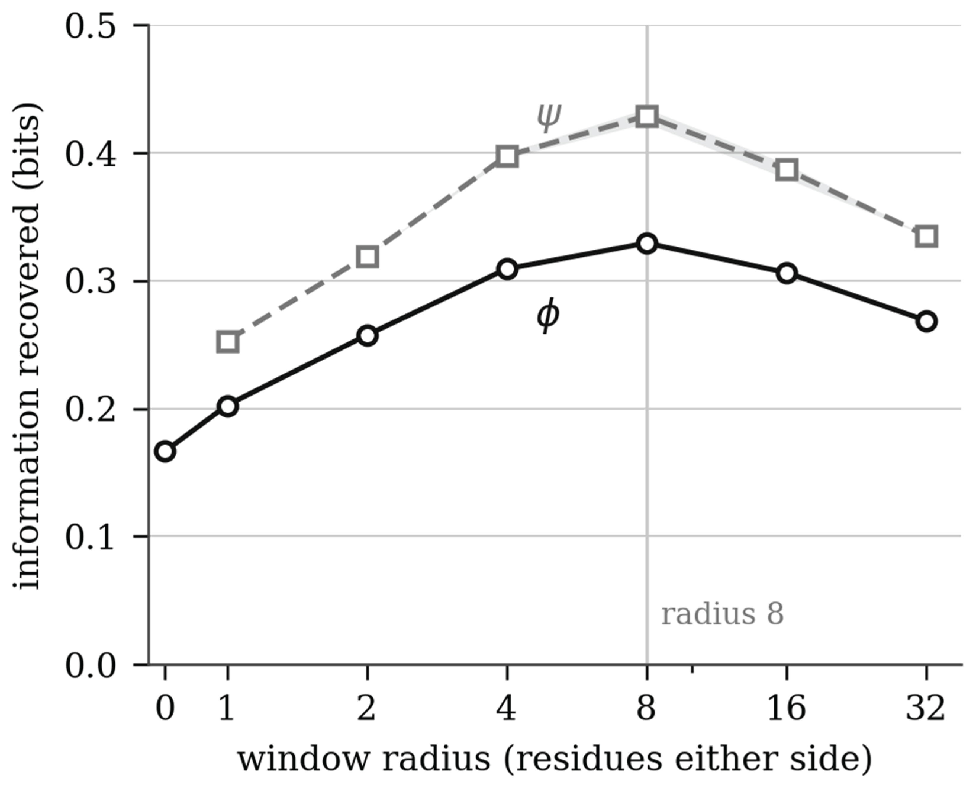
Figure 2.
Bias-corrected pairwise mutual information against sequence separation d. Bias-corrected pairwise mutual information between the residue at sequence separation d and φ, estimated from 542,144 training residues with no model, against a within-chain permutation null. The centre bar (d = 0, the residue’s own identity) is clipped. The corrected estimate falls to the null level by |d| ≈ 10 downstream and ≈ 8 upstream, matching the radius at which the trained model peaks.
Figure 2.
Bias-corrected pairwise mutual information against sequence separation d. Bias-corrected pairwise mutual information between the residue at sequence separation d and φ, estimated from 542,144 training residues with no model, against a within-chain permutation null. The centre bar (d = 0, the residue’s own identity) is clipped. The corrected estimate falls to the null level by |d| ≈ 10 downstream and ≈ 8 upstream, matching the radius at which the trained model peaks.
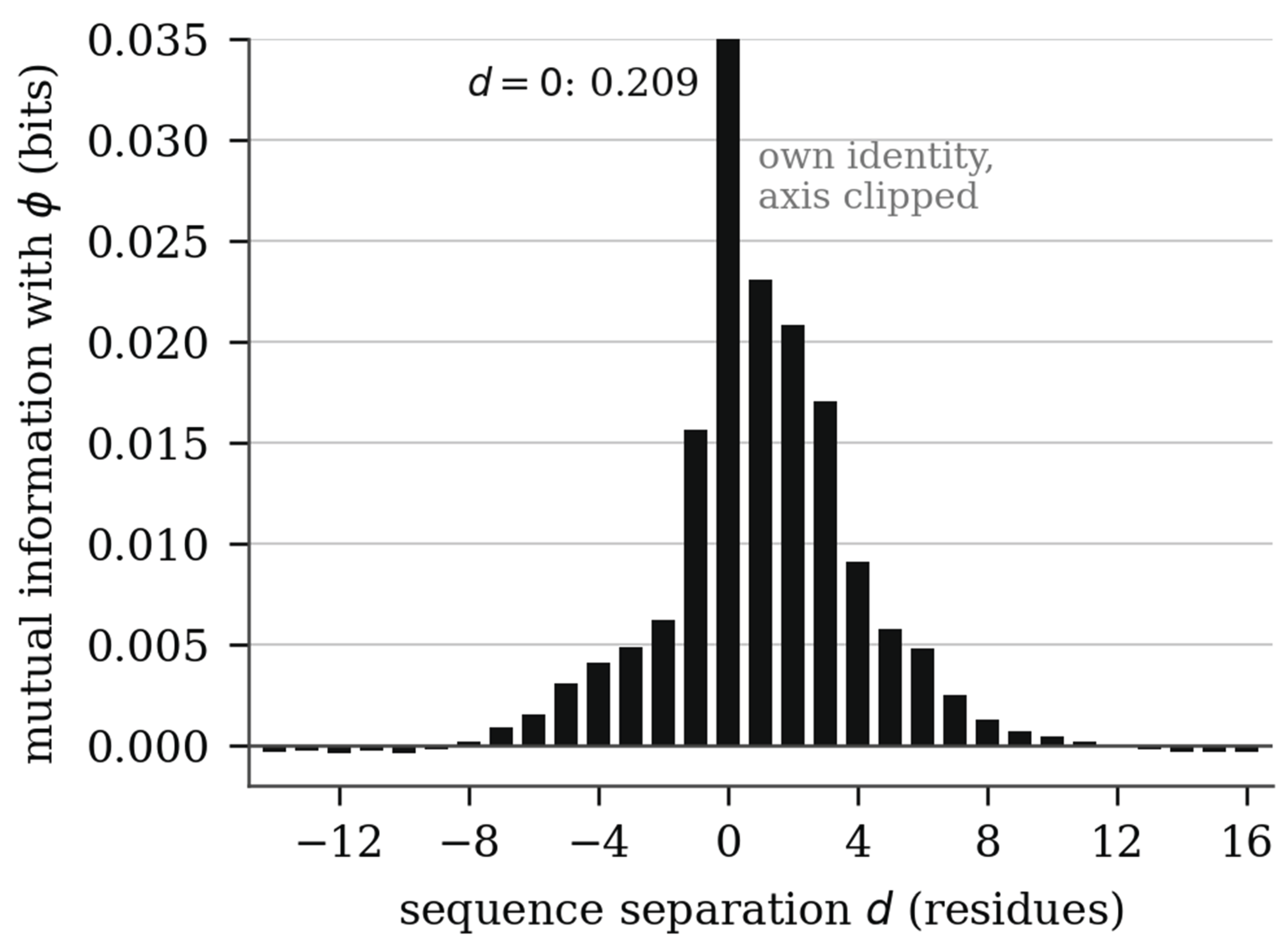
Figure 3.
Information gained beyond each class’s own φ marginal, training and held out, 2026 dataset. Information gained beyond each secondary-structure class’s own φ marginal, on training and held-out data of the 2026 dataset, with the percentage retained. Coil carries three times what helix carries, but all three classes retain close to ninety per cent of what they fit. The helix deficit is therefore a failure to generalise, not a failure to fit.
Figure 3.
Information gained beyond each class’s own φ marginal, training and held out, 2026 dataset. Information gained beyond each secondary-structure class’s own φ marginal, on training and held-out data of the 2026 dataset, with the percentage retained. Coil carries three times what helix carries, but all three classes retain close to ninety per cent of what they fit. The helix deficit is therefore a failure to generalise, not a failure to fit.
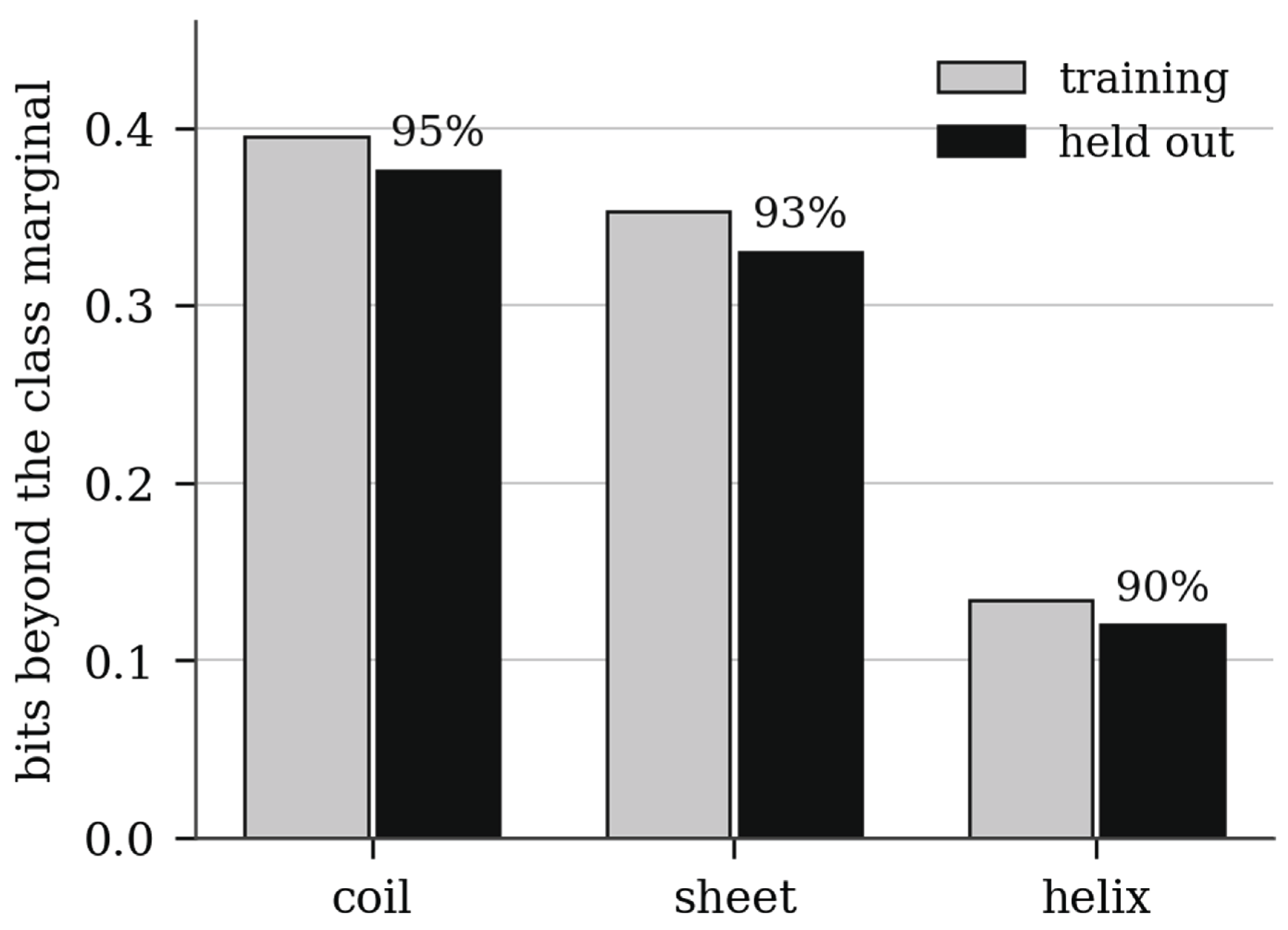
Table I.
Information recovered about φ (bits, held-out test split) against window radius, at four angular resolutions. Each column is scored against the H₀ of its own bin width.
Table I.
Information recovered about φ (bits, held-out test split) against window radius, at four angular resolutions. Each column is scored against the H₀ of its own bin width.
| Radius | 5° (72 bins) | 10° (36 bins) | 20° (18 bins) | 30° (12 bins) |
| 2 | 0.244 | 0.257 | 0.291 | 0.292 |
| 4 | 0.303 | 0.309 | 0.343 | 0.335 |
| 8 | 0.313 | 0.330 | 0.353 | 0.355 |
| 16 | 0.281 | 0.306 | 0.332 | 0.329 |
Table II.
Protein-level bootstrap on the held-out test split, 20,000 paired resamples.
| Quantity | Point estimate | 95% CI | P(≤ 0) |
| bits at radius 0 | 0.166 | 0.112 – 0.219 | |
| bits at radius 8 | 0.330 | 0.265 – 0.392 | |
| bits at radius 32 | 0.269 | 0.209 – 0.329 | |
| radius 8 − radius 0 | +0.163 | 0.143 – 0.183 | < 0.0001 |
| radius 8 − radius 32 | +0.060 | 0.047 – 0.073 | < 0.0001 |
Table V.
Information gained beyond each class’s own φ marginal, held-out test split of the 2026 dataset. Retention is the signed ratio of the held-out gain to the training gain.
Table V.
Information gained beyond each class’s own φ marginal, held-out test split of the 2026 dataset. Retention is the signed ratio of the held-out gain to the training gain.
| Class | n train | n held out | Training | Held out | Retained |
| coil | 916,906 | 111,722 | +0.395 | +0.376 | 95% |
| sheet | 212,086 | 25,422 | +0.353 | +0.330 | 93% |
| helix | 533,754 | 63,263 | +0.134 | +0.120 | 89% |
Table VII.
test split against the fraction of the training split the model was allowed to see. Helix transfer is positive at every rung, including one where the model sees fewer helix residues than the radius-sweep dataset contains.
Table VII.
test split against the fraction of the training split the model was allowed to see. Helix transfer is positive at every rung, including one where the model sees fewer helix residues than the radius-sweep dataset contains.
| Training data | helix residues seen | coil | sheet | helix |
| 12.5% | 66,719 | +0.306 | +0.237 | +0.054 |
| 25% | 133,438 | +0.332 | +0.272 | +0.068 |
| 50% | 266,877 | +0.351 | +0.282 | +0.113 |
| 100% | 533,754 | +0.376 | +0.330 | +0.120 |
| radius-sweep set, all | 175,700 | +0.298 | +0.112 | −0.012 |
Table VIII.
Joint φ/ψ modelling against an independent control, held-out test split. Both arms are scored on the 16,585 residues at which φ and ψ are both defined, a slightly smaller set than elsewhere in the paper, which is why the φ marginal reads 0.335 rather than the 0.330 of Figure 1.
Table VIII.
Joint φ/ψ modelling against an independent control, held-out test split. Both arms are scored on the 16,585 residues at which φ and ψ are both defined, a slightly smaller set than elsewhere in the paper, which is why the φ marginal reads 0.335 rather than the 0.330 of Figure 1.
| Quantity (bits, test) | Coupled | Independent |
| φ marginal | 0.335 | 0.335 |
| ψ marginal | 0.410 | 0.418 |
| joint | 0.469 | 0.020 |
Disclaimer/Publisher’s Note: The statements, opinions and data contained in all publications are solely those of the individual author(s) and contributor(s) and not of MDPI and/or the editor(s). MDPI and/or the editor(s) disclaim responsibility for any injury to people or property resulting from any ideas, methods, instructions or products referred to in the content. |
© 2026 by the authors. Licensee MDPI, Basel, Switzerland. This article is an open access article distributed under the terms and conditions of the Creative Commons Attribution (CC BY) license (http://creativecommons.org/licenses/by/4.0/).
Copyright: This open access article is published under a Creative Commons CC BY 4.0 license, which permit the free download, distribution, and reuse, provided that the author and preprint are cited in any reuse.