

Submitted:
01 September 2026
Posted:
01 September 2026
You are already at the latest version
Abstract
A quantum jump trajectory is a discrete-event process in the literal sense: coherent evolution between jumps, a waiting time drawn from the decay of the no-jump norm, a channel selection at the jump. We take this correspondence in both directions. First, we build a monitored quantum laboratory (a driven emitter, detectors with efficiency and dead time, a click-driven feedback controller) inside a verification-first discrete-event engine that machine-checks the event structure and the bookkeeping on every transition, validated against exact finite-horizon renewal expectations and against QuTiP. Second, we import a comparison discipline that is standard in discrete-event simulation and that we did not find in the quantum trajectory literature: common random numbers. Addressing the randomness by event ordinal keeps two protocol arms on identical draws until their event histories diverge, and a mechanical audit verifies the pairing rather than assuming it. Pairing pays in proportion to trajectory alignment: for close protocol variants, where the selection decision is hard, the variance of the estimated protocol gap falls by a factor of 40 or more (replicated across five seeds), and the paired design resolves a 0.7% rate difference at \(n = 400\) trajectories that the unpaired analysis of the same data cannot. Against the Fisher information of the click record, that paired design recovers about a tenth of the achievable precision at the count endpoint and the unpaired design under two percent, with the remaining gap attributable to the endpoint rather than the pairing. Two physics results follow. Dead-time losses for antibunched light sit well below the textbook Poisson correction, an effect reaching 21% that we compute exactly for resonance fluorescence and reproduce within the measurement intervals. And the rate-optimal feedback pulse after a click is not a \(\pi\) pulse, and not because of latency: the mean wait is exactly \(a_0 + a_1\cos\theta + a_2\sin\theta\) for every drive, detuning and latency, which puts the zero-latency optimum at our drive at exactly \(3\pi/4\) and the deficit of the \(\pi\) pulse at exactly \(\sqrt{2} - 1\), both confirmed by measurement at the shortest latency we can represent. Latency lowers the optimum further, and \(\pi\) is recovered only as the drive weakens. The optimum does not maximize post-pulse excitation, because the waiting time depends on coherence with the drive, not population alone.
Keywords:
quantum trajectories
; quantum jump unraveling
; common random numbers
; variance reduction
; discrete-event simulation
; photon antibunching
; detector dead time
; resonance fluorescence
; quantum feedback control
; simulation verification
1. Introduction
An open quantum system under continuous monitoring evolves coherently between detection events and jumps at random times. The quantum jump unraveling of the master equation makes this structure exact: the waiting time until the next jump is drawn from the decay of the no-jump norm, and the jump then selects a dissipation channel [1,2,3,4]. Radaelli, Landi and Binder made the correspondence explicit by recasting jump trajectories as a Gillespie process [5]: the same algorithm that underlies chemical kinetics [7] and, in its scheduling structure, discrete-event simulation generally. Under counting-type unravelings the detection record is not merely simulable by discrete events. It is a marked point process exactly, and not as an approximation of some underlying continuous description: it is what the detector produces. (Diffusive unravelings, homodyne and heterodyne, are outside this correspondence and outside this paper.)
This paper takes the correspondence seriously in both directions, and each direction produces results the other cannot.
In one direction, we build the laboratory inside a discrete-event engine designed for verification (Section 2). The dominant modelling errors in this domain are structural, not numerical: a decay path omitted from the operator set, or a detector inefficiency modelled as a loss channel and then also counted in the total rate. Neither produces a crash or an implausible trajectory. Both produce a smooth, converged, tightly error-barred, wrong ensemble average, and more replications never catch them. What catches them is exhaustive bookkeeping: machine invariants checked on every transition of every trajectory (the channel rates sum to the declared decay; the conditional state has unit norm at every anchor; photons reconcile exactly against clicks, inefficiency misses, and dead-time absorptions; every click is consumed by exactly one controller rule), and load-time gates on the declared wiring (every jump channel has exactly one detection destination; every emitted event kind is covered). The engine machine-checks the event structure and the bookkeeping, not the Hamiltonian: the coherent evolution between jumps is closed-form numerics that no model checker touches, and we validate it instead against analytic known answers and against QuTiP [9] (Section 3).
In the other direction, we import the discrete-event community’s standard comparison discipline into a field that does not use it. The decision problem in monitored quantum systems is protocol selection: which control pulse, which feedback policy, which measurement strategy performs best under realistic detector imperfections. Current practice simulates independent trajectory ensembles per protocol and compares their means [9], which discards the fact that both protocols face the same stochastic environment. Common random numbers (CRN) make the comparison paired [13,14,15]: the shared stochastic backbone cancels out of the difference. We are not aware of any use of this technique in the quantum trajectory literature (Section 6), and the nearest quantum relative, correlated sampling in ground-state quantum Monte Carlo [11,12], lives in a different domain. Our implementation addresses every random draw by event ordinal (the k-th jump, the k-th detector arrival), so two protocol arms consume identical uniforms up to the ordinal where their event histories diverge, and a mechanical audit verifies after the fact that the shared draws were byte-identical while reporting the arm-only tails (Section 5).
Our contributions:
- 1.
- A verified event-structure laboratory for monitored quantum systems (Section 2, Section 3). Gillespie waiting times computed in closed form, detector dead time and inefficiency as journaled bookkeeping, click-driven feedback with stale-jump cancellation, all invariant-checked per transition; validated against exact finite-horizon renewal expectations and QuTiP (twelve assertions on three levels, all passing), with the laboratory’s own estimator defect, caught by external review, as the demonstration that the target defect class is real (Section 3.1).
- 2.
- An exact dead-time correction for antibunched resonance fluorescence, for an effect reaching 21% (Section 4). The textbook non-paralyzable correction assumes Poisson arrivals. Sub-Poissonian arrivals are regularized, fewer land in the dead window, and the measured rate sits up to 21% above the Poisson prediction. That dead time modifies non-Poisson counting statistics is established; what we add is the exact delayed-renewal expectation for this source, reproduced by the laboratory across to 8 decay times.
- 3.
- Paired trajectories, with the audit as the instrument (Section 5). The variance of the estimated protocol gap falls by or more for near-identical protocols (40 to 430 across five seeds: the ratio itself is heavy-tailed at the smallest gap, and we report it as a floor), decaying to as the protocols diverge, and the CRN audit’s shared-stream ledger measures the alignment mechanism directly, closely enough that, calibrated on one protocol family, it predicts another family’s variance ratios to a median factor of (Section 5.5). At every seed the paired design resolves protocol differences the unpaired analysis of the same data cannot.
- 4.
- The rate-optimal feedback pulse is not , and not because of latency (Section 5.4). The mean wait after the pulse is exactly, for every drive, detuning and latency, so the optimum is and equals only when . At our drive, which is the exceptional point of the effective Hamiltonian, the zero-latency optimum is exactly and the pulse gives up exactly of the rate; the measurement at the shortest representable latency returns and 40% ( is recovered only as , which is the statement ); latency lowers the optimum along a measured curve ( at , at ; measured baselines are the prediction rounded to the grid of the sweep that produced them); and the optimum does not maximize post-pulse excitation. Locating one optimum took paired trajectories per arm; the unpaired equivalent would need roughly an order of magnitude more.
2. Model and Simulation Framework
2.1. Physics and the Gillespie Step
The system is a driven two-level emitter under photon counting, in the rotating frame:
with total decay split across K detection ports. Every result in this paper is on resonance, . Between events the conditional (unnormalized) state evolves under as , computed in closed form by complex eigendecomposition. No integrator and no tolerance knob appear anywhere. The no-jump survival is , monotone from 1 toward 0 under driving.
The Gillespie step [5,7]: at every anchor (the start of time, each jump, each control pulse) the emitter receives two uniforms and decides deterministically. The waiting time solves by bracket and bisection on the closed form. The channel follows from against the weights ( is drawn even when : the fixed-draw rule below). The jump is then scheduled as a future event. After a jump the state is exactly. A control pulse arriving before the scheduled jump propagates the conditional state to the pulse time, applies its unitary, cancels the pending jump, and re-draws: the old waiting time was conditioned on the pre-pulse state, and reusing it would be a conditioning error that no ensemble average would flag. Time is discretized at decay times per tick and waiting times round to at least one tick. The suite bounds the resulting bias by halving the tick and re-running the known-answer gates; it sits below the statistical floor of every measurement in this paper.
2.2. Machine Architecture, Invariants, and Randomness Allocation
The laboratory is composed from three machine types. The emitter holds the conditional state and the declared channel partition. The photodetector (one per port) applies efficiency and non-paralyzable dead time : a photon arriving during the dead window is a journaled refusal with a named reason, counted in absorbed, never silently dropped; a live arrival is resolved against one uniform, becoming a click (which extends the dead window and notifies the controller) or a counted miss. The controller consumes clicks under a declared policy: none, or pulse-on-click with a declared angle, latency, and refractory window. A click in the refractory window is a journaled refusal. The topology declares which dissipation channel is monitored by which detector and which click drives which controller action, and the engine’s load gates check the wiring is total.
The division of responsibilities defines the architecture: responders draw, machines decide, the kernel schedules. Machines own no randomness. A responder hands the emitter its two uniforms at the current jump ordinal, from a named stream (jump:{node}:n{k}); a second responder hands each detector one uniform per arrival (eff:{node}:n{k}). Two rules make this a comparison instrument rather than a convenience. The fixed-draw rule: every ordinal consumes the same number of uniforms in every scenario, unconditionally. The ordinal-addressing rule: streams are named by event index, not by simulation time, so two protocols under one seed share their stochastic backbone draw for draw until their event histories diverge. Section 5 builds on both.
The bookkeeping invariants run on every transition of every trajectory: the channel rates sum to the declared exactly; the anchor state has unit norm; photons = clicks + misses + absorptions + in-flight resolutions, exactly; clicks seen = consumed + refused; pulses fired never exceed clicks consumed. Across every run reported in this paper these invariants evaluated with zero violations, and each run reproduces its journal digest byte for byte from its content-addressed identity (world hash, scenario hash, seed, replication index).
3. Verification Against Known Answers and QuTiP
The two-level emitter is chosen because its ground truth is independently known. The steady state gives the photon rate with , and renewal theory makes the mean inter-jump waiting time exactly . At a finite horizon the correct comparison target is not R itself: for an ordinary renewal process started at a renewal point, , and for sub-Poissonian intervals () that constant is negative. We therefore gate against the exact finite-horizon renewal expectation , computed deterministically from the no-jump survival by a grid-and-FFT renewal sum (make_figs.py). Table 1 shows the laboratory against both targets at trajectories of decay times per cell (± values here and throughout are SE, ≈95% CIs).
3.1. Case Study: An Estimator Bias Identified by External Review
The first draft of this paper carried a rate estimator that normalized clicks by the time of the last recorded event rather than by the declared horizon. For a renewal process that is the classic inspection-paradox estimator: , with the mean backward recurrence time, a deterministic to bias in every absolute rate. Every gate passed anyway: at the bias sat inside SE, and three same-sign one-sigma excesses were absorbed by three separate error bars. This is exactly the defect class the introduction names (a smooth, converged, tightly error-barred, slightly wrong number), and it was caught not by more replications but by external review computing the backward-recurrence correction from the machine’s own survival function and reproducing the excess to four decimal places. The fix is one line (divide by the horizon); the residual finite-horizon physics is the renewal constant above, now part of the gates; and the paired-comparison results of Section 5 moved by less than a tenth of their interval widths, because the bias was common mode across arms.
We retain the episode because of what it delimits. The defect did not live in a machine: it lived in a probe, and probes are pure folds over the journal that sit outside the invariant perimeter entirely. The machine invariants cannot see an estimator, so no amount of per-transition checking was ever going to flag this, and the cross-validation did not either, because QuTiP was refereeing the same biased quantity. The constructive lesson is that estimator identities are themselves checkable, and cheaply: the horizon-normalized and last-event-normalized rates differ by precisely the bias in question, so their discrepancy is a standing gate, and the laboratory now carries it. The episode supports a narrow claim: because the event structure, the draw sites, and the estimator were all declared artifacts rather than implementation details of a bespoke simulator, an external reader could localize the defect analytically from the machine’s own survival function, without rerunning anything. Reproducibility of the event structure is what made the error findable by someone other than its author.
Figure 1 shows the full waiting-time distribution at : the antibunching hole at the origin (: a jump resets the emitter to and re-emission requires re-excitation [3,18]), the Rabi lobe structure under the decay envelope, and the same-mean exponential reference cutting through both. None of this structure is put in by hand. It emerges from the event process, which is the point of validating against it.
QuTiP is the external referee [9] (worlds/monitored/qutip_cross.py), on three levels mirroring the cross-validation discipline of our companion study [24]. The twelve assertions counted here are the QuTiP comparisons only; the laboratory’s own test suite is separate and is described under Reproducibility. Analytic: QuTiP’s steadystate matches the machine’s closed form to at all three drives. Distributional: collapse times recorded by mcsolve give waiting-time means and short-wait fractions consistent with the laboratory’s (for example 2.240 versus 2.252 at ). Statistical: the master-equation click rates sit inside the laboratory’s CIs at every drive. Twelve assertions across the three levels, all passing. Detector dead time and click-triggered feedback are outside QuTiP’s machinery, which is precisely the gap the laboratory exists to fill; their referees are the exact renewal expectations of Section 4 and Section 5.4.
One boundary should be stated where the reader will look for it. The renewal-expectation curves in Figure 5 and Figure 2 are computed in an independent numpy implementation of the closed forms (a separate codebase from the machine’s JavaScript), so agreement checks both implementations of the model. It does not check the model against nature; that is what the analytic steady state, QuTiP, and the antibunching structure of Figure 1 are for. And all parameter sweeps in this paper run a single detection port (); the multi-channel partition machinery is exercised by the load gates, the unit suite, and one reported two-port measurement (k2-check.mjs: ports at of , per-port click rates and against expected shares and of the exact finite-horizon expectation, photons reconciling exactly per port in all 40 runs, zero invariant findings; and the paired latency comparison of Section 5.3 rerun on the two-port world resolves at a variance ratio with the audit verifying both detectors’ streams).
4. Antibunched Light and the Dead-Time Formula
Every photon-counting experiment corrects for detector dead time. The standard non-paralyzable correction [19] is
That formula assumes Poisson arrivals. That dead time modifies the counting statistics of non-Poisson light is an established literature: dead-time-corrected photocounting distributions go back to Cantor and Teich [20], dead-time-modified count moments and their observation to Vannucci and Teich [21], and corrections for correlation measurements through modern single-photon detectors [22,23]. Clark et al. model count-rate saturation for bunched, Poissonian, and antibunched sources through detectors with a measured efficiency-recovery profile [23]; our step-function dead window is the non-paralyzable idealization of that recovery, and the machine’s journaled design would absorb a graded profile as a time-dependent . The light in this laboratory is antibunched: arrivals are regularized and short gaps are suppressed (Figure 1), so fewer photons arrive inside the dead window, and the loss is smaller than Eq. (2) predicts. The contribution here is not the existence of the effect but its exact, gate-grade computation for resonance fluorescence, verified in a laboratory where dead time is a first-class journaled event.
The exact prediction is renewal-theoretic. At the jumps form a renewal process with waiting density from . An accepted click at a renewal point opens a dead window ; the next accepted click is the first jump after it, so the inter-accepted intervals are i.i.d. with , Y the forward recurrence time at lag , while the first interval of a trajectory is an ordinary wait (the first click pays no dead time). The accepted-click process is therefore a delayed renewal process, and we compute its exact finite-horizon expectation by the same grid-and-FFT renewal sum as the gates of Section 3. Figure 2 shows the laboratory against this prediction and against Eq. (2) across to 8 decay times: every measured point sits within interval half-widths of the exact curve, and above the Poisson formula everywhere, by up to 21% at , converging only in the long-dead-time limit where both scale as .
The practical implication is direct. Dead-time corrections calibrated on Poisson sources over-correct antibunched sources. The size of the effect at is tens of percent, and the correction requires the waiting-time distribution, not just the rate. The laboratory computes it because dead time is a first-class, journaled event in the detector machine, not a post-hoc analysis step.
5. Paired Trajectories
5.1. Paired-Comparison Method and Audit Procedure
Comparing feedback protocols with independent ensembles estimates with variance . Pairing replication i of protocol A with replication i of protocol B on the same draws subtracts [13,15]. The technique is decades old in operations research. It is not guaranteed to be a gain: the classical theory gives monotonicity conditions under which the covariance is positive [13], and a recent planning result exhibits decision processes where full pairing increases the variance [17]. Nothing forces for quantum protocol arms either. The variance ratio is therefore a measured output of every comparison in this paper. Every ratio we measure is above one. The quantum trajectory literature evaluates protocols on independent realizations (Section 6), and the reason is partly mechanical: pairing requires that “the same randomness” be well defined across two systems whose event counts differ, and a global RNG sequence loses alignment at the first divergent event.
Ordinal stream addressing solves the alignment problem. The k-th jump decision of the emitter draws from a stream named by k in both arms; the k-th arrival at a detector likewise. Two protocols under one seed therefore consume identical uniforms at every ordinal both of them reach. When the histories diverge (one protocol jumps more often), the arms consume different total draw counts, and that is not an error: it is a measured property of the comparison. After every paired run the engine’s CRN audit compares the two arms’ per-stream draw ledgers and refuses the paired analysis on any mismatch, while reporting the arm-only tails.
Byte-identity of shared streams in a correct engine is close to tautological, since streams derive deterministically from seed and name. The audit’s content is threefold: it catches fixed-draw-rule violations, an arm whose draw count per ordinal became state- or scenario-dependent, which is exactly the silent CRN-killer in hand-rolled trajectory pairings; it catches ordinal misaddressing and stream-name collisions; and its shared/arm-only ledger is the alignment instrument of Section 5.3. A mutation test in the laboratory’s suite injects a responder that consumes one extra uniform past a scenario-controlled jump ordinal (both arms still run; both produce plausible physics), and the audit refuses the comparison with the mismatched streams named (CRN_AUDIT_FAILED, monitored.test.mjs).
Protocol arms are scenario documents (data, not code), so a protocol comparison is a declared experiment: paired scenarios, a declared endpoint (the accepted-click rate), paired-t intervals, and the audit, in one report.
5.2. Distant Protocols: A Negative Result
Pairing is not automatically beneficial, and the first measurement establishes its scope. Comparing feedback off against pulse-on-click at (), the paired and unpaired interval widths nearly coincide: variance ratios 1.1 to 1.4 across latencies. The reason is physical. The protocols differ so strongly (the pulse arm emits three times faster) that their event histories decorrelate after the first click, the outcome correlation collapses, and the covariance term buys almost nothing. The audit ledger reflects this directly: 81 shared streams against up to 380 arm-only streams. For protocol screening across qualitatively different policies, independent ensembles are essentially optimal. This is the scope boundary of the method.
5.3. Close Protocols: The Variance Curve
The selection decisions that matter are between close variants: this latency against that one, this pulse angle against that one. There the trajectories stay aligned and pairing pays exactly where the decision is hard. Figure 3 sweeps the latency gap between two pulse-on-click protocols at : the variance ratio falls monotonically from at decay times to at , and the audit’s shared-stream count falls along the same curve (319 shared streams per pair at the smallest gap, 171 at the largest). The arm-only tails are instructively asymmetric (Figure 3b): the baseline-only count grows (150 to 254) while the variant-only count collapses toward zero (90 to 3), because the slower high-latency arm reaches fewer event ordinals and its consumed set becomes a near-subset of the baseline’s. Protocol distance shows up not as symmetric divergence but as one arm’s ordinal range outrunning the other’s, and the ledger distinguishes the two. For close protocols, correlation, alignment, and the audit ledger are three views of the same phenomenon, and Section 5.5 turns the third into a quantitative predictor of the first.
The operational cell is : the paired estimate of the protocol gap is , resolved decisively, while the unpaired analysis of the same 800 trajectories reports and resolves it only marginally (the point estimate exceeds the interval by a factor of 1.3); at the paired design resolves (a 0.7% relative difference) where the unpaired interval contains zero with room to spare. In terms of computational cost, an unpaired study would need at least the trajectories to make the decision the paired study makes at . One caution on breadth: the sweep runs eight gaps at with no multiplicity correction; the resolved/unresolved contrasts quoted here are the two pre-declared headline cells, not the product of multiple-comparison selection.
The should be read as a floor, not a point value, and the distinction is itself a measured property of the method (seed-rep.mjs). Replicating both headline cells across five seeds leaves the paired point estimate essentially unchanged ( to at ) and the decision pattern stable within each cell: at the paired design resolves at every seed and the unpaired design at none, while at both resolve at every seed. The marginal unpaired resolution reported above is a property of that gap, not of this paper’s seed. The variance ratio at the smallest gap ranges from 40 to , with this paper’s seed at the minimum. The mechanism is the same alignment physics read at one more level: at most replication pairs never invert their event order and contribute nearly zero difference, so the paired variance is carried by the few pairs that do, and how many such pairs a seed contains fluctuates. The difference distribution is heavy-tailed exactly where pairing pays most, which is also a caution about paired-t intervals in that regime; at the operational gap the ratio is stable, 20 to across the same five seeds.
5.4. The Pulse-Angle Optimum Is Not , Even at Zero Latency
The applied payoff is protocol optimization. The intuitive click-triggered protocol is a pulse: the emitter just jumped to , so re-excite it fully. The intuition fails in two separable ways, and neither is a latency artifact.
The first failure needs no latency at all, and it is available in closed form. Write the post-pulse state as , with and the normalized conditional state at the end of the latency window. The no-jump survival , with , is a quadratic form in , so the half-angle products collapse onto and the mean wait is
with , and , all evaluated in and independent of . Equation (3) is exact for every drive, detuning and latency. The mean cycle is , so the rate optimum and its value are
and if and only if . The coefficient carries the off-diagonal response to , and it vanishes only when the pre-pulse state leaves the drive no dipole to act on. That is the first failure in one line. The pulse is rate-optimal exactly when the drive does no work during the wait, and the weak-driving recovery of is the statement : runs from at to at (Figure 4b). Coherence with the drive, not population, sets the re-emission clock.
At the operating drive the coefficients are elementary, because is the exceptional point of : the eigenvalues coalesce, the propagator acquires a nilpotent term, and the survival is rather than a sum of two exponentials. At this gives , so
and the pulse gives up exactly of the rate. The zero-latency optimum is , not a value near it.
Two statements bound what this covers. Equation (3) is the asymptotic cycle; the finite-horizon optimum from the renewal sum of Section 3 at sits above it uniformly in L, inside the grid of the sweeps. And because Figure 4b carries from to across the exceptional point with no feature in , the structure of the optimum is not an artifact of operating there.
The engine represents a latency of one tick (, the quantization floor), so the zero-latency limit is measurable and not merely derived. At one-tick latency (theta-zero.mjs, /arm) the protocol is resolved above both declared neighbors ( at , at ) and above the pulse by , a 40% rate deficit for the textbook choice against the derived 41.4%.
The second failure is the latency pre-rotation. During L the conditional state evolves under the drive and acquires part of the rotation, acquires a dipole, grows, and falls along a monotone curve, from at to at (Figure 4a and Table 2). The measurement tracks the curve (theta-L.mjs, /arm): at , , and the predicted-optimum baseline beats both its neighbors by the paired design (all six comparisons resolved below, the tightest at ), just as it does at the operating point of Figure 5.
At the operating point (, ) the click process under the protocol is a delayed renewal process (a long un-pulsed first wait from , then cycles of length ), and its exact finite-horizon expectation, computed as in Section 3, has its maximum at . The post-pulse excitation peaks elsewhere, near (Figure 5b): the rate optimum deliberately sacrifices population for coherence with the drive.
Figure 5a shows the measurement: with the predicted optimum as the paired baseline, every measured angle is resolved below it, including the two pre-declared nearest neighbors, at (a 0.5% relative difference) and at (the other five angles are also resolved, but the localization claim rests on the two declared neighbors, so the seven tests are not the product of multiple-comparison selection). The whole optimization cost trajectories per arm; the variance ratios against the baseline run 3 to 17 across the sweep, with the two nearest neighbors at 16 and 17: an unpaired-equivalent cost of roughly 7,000 trajectories per arm for the decisions that localize the optimum.
The absolute agreement with the theory curve is weaker than the localization result, and it separates into two parts. Every measured point at sits within one interval half-width of the exact expectation ( to half-widths). All eight residuals are positive, but the eight arms are paired against a common baseline, so they carry one common-mode realization between them rather than eight independent ones. Reading the paired differences separates the two contributions.
A common-mode offset of to is present at every angle, and the during-latency emission branch accounts for it: a jump inside the latency window (probability per cycle) yields an extra counted click and delivers the pulse to a freshly reset state, contributing to to the rate across the sweep. Net of that offset the paired differences match the theory to within from to , which is the range the localization claim occupies.
A separate effect appears at , reaching in the paired difference at . It does not follow the angle. It follows post-pulse excitation, peaking where the excitation peaks ( at ) and falling back at , where the excitation falls to . Three candidate sources are excluded. Quadrature error: Richardson extrapolation at and at agrees to five decimals at every angle, and the residual grid drift falls with while the discrepancy grows. Solver tolerance: the survival inversion runs bracket doubling then bisection to machine precision. Tick quantization: the probability of a wait shorter than half a tick is even at full inversion, an order of magnitude too small and of the wrong sign. The effect is not identified. The one-tick-latency arms show an offset of the opposite sign (measured 2.5% below the prediction).
These bound what the theory comparison establishes: the two implementations of the renewal model agree with each other to quadrature accuracy, and the machine reproduces the model to in paired difference across the localization range and to about 1 to 2% in absolute rate at the largest angles. The localization claims are unaffected, because they rest on paired differences within a single arm-pair, where a common-mode model offset cancels; this is the same cancellation the paper’s method exploits throughout, here visible as a property of the comparison rather than of the model.
5.5. How Much of the Achievable Precision Does Pairing Recover?
Section 5.3 and Section 5.4 report variance ratios against the unpaired design, which answers what pairing buys relative to current practice but not what it leaves on the table. The click record is a renewal process with a known interval density, so the question has an absolute answer: the Fisher information of that record bounds any estimator of the protocol gap, and the achieved variance can be placed against it.
For the pulse-on-click protocol the inter-click interval is , with drawn from the waiting density of the pulsed state . The interval density depends on the latency twice over, by translation and through the pre-pulse evolution, so the information is not the trivial shift information. At the operating point (, , ) numerical quadrature on the closed forms of Section 3 gives per interval and, at intervals per trajectory, per trajectory. By the delta method the Cramér-Rao floor on the standard error of the rate gap at is .
Table 3 places four estimators of the same decision against that floor. The rows between the two extremes are computed in an idealized renewal replica in which both arms draw the same uniform at every ordinal, which is the strongest coupling ordinal addressing can express. The replica is not a prediction of the laboratory: it reproduces the laboratory’s baseline rate to , its paired gap to and its unpaired standard error to , but its arms never lose alignment, so its paired row is a ceiling rather than a measurement.
For the two coupled rows the third column is a ratio and not an efficiency. A coupled design is a stronger experiment than the independent-arms floor describes, so the paired score at 68% of that floor does not license the reading that the estimator is close to optimal: the bound for a coupled design sits lower, and where it sits is the open question at the end of this section.
Two separate losses account for the distance between current practice and the bound, and the table separates them.
The first is the endpoint. The count is a lossy summary of a renewal record: it discards the interval structure that carries most of the information about the latency. Replacing the count by the score , at the same coupling and the same n, moves the estimator from 36% to 68% of the bound, a further factor of in variance. Pairing and the endpoint are therefore independent axes: pairing removes the common noise, the endpoint decides how much of the remaining signal is read.
The second is alignment, and the laboratory already measures it. Under ideal coupling the paired count reaches a variance ratio of 451; the laboratory achieves 40 at the same gap, and the shortfall is trajectory divergence. That invites reading the audit ledger of Section 5.3 quantitatively rather than as illustration. Across all seventeen paired comparisons in this paper, taking the overlap relative to the larger arm, , the variance ratio is exponential in the overlap (Figure 6):
The fit is taken over the fourteen close-protocol comparisons, but the substantive test is out of sample. The pulse-angle family occupies , inside the latency family’s , so the relation can be calibrated on the latency family alone and used to predict the angle family cold. Fitted on the eight latency comparisons, Eq. (6) predicts the six angle comparisons to a median factor of and a worst case of , across a perturbation type the fit never saw: a latency change translates the interval density, a pulse-angle change reshapes it. The ledger is therefore not merely a correctness check on the pairing. It is a predictor of what the pairing will buy, and it carries across the kind of perturbation within a calibrated range of overlap.
That range qualification is load-bearing. Fitted separately the two families have slopes (latency, ) and (angle, ), differing by standard errors, so they do not lie on a common line; predicting in the other direction, out of the angle family’s narrow span, degrades to a median factor of . Within each family the comparisons also share a baseline arm, so the fourteen points carry fewer independent degrees of freedom than their count suggests. What the measurement supports is an interpolating predictor over a calibrated range of overlap, not a universal exponent.
The exception is the distant-protocol family of Section 5.2, which sits off the line and whose measured ratios fall below the prediction by about half at comparable overlap. That is the regime in which the arms differ threefold in rate, and it is the regime the same section already recommends running unpaired, so the predictor fails exactly where its answer would not be used.
Two consequences follow. Because the dependence is exponential, overlap is a sensitive design lever: the difference between and is a factor of four in the achievable precision, which argues for choosing protocol parameterizations that keep arms on shared ordinals. And because the relation is calibrated rather than derived, a single pilot pair fixes and predicts the benefit of a planned comparison before the full study is committed. Deriving Eq. (6) from the coupling structure, rather than fitting it, remains open.
Three scope statements. The information is the classical Fisher information of the jump record under this unraveling, not the quantum Fisher information over all measurement strategies; the latter is the subject of Radaelli et al. [6], whose renewal and Markov-chain machinery computes it properly, and whose bound would sit below ours. The quadrature uses the ordinary-renewal approximation, so the delayed first interval and horizon censoring enter at order . And the bound is stated for independent arms; establishing the corresponding bound for a coupled design, where the shared randomness is part of the experiment rather than a nuisance, is the open theoretical question this section raises.
6. Related Work
Quantum jump unravelings go back to Dalibard, Castin and Mølmer [1,2] and Carmichael [3], with Plenio and Knight’s review [4] and Wiseman and Milburn’s treatment of measurement and feedback [8] as standard references; QuTiP’s mcsolve is the field’s reference implementation [9]. Radaelli, Landi and Binder recast the jump unraveling as a Gillespie process [5]; we build directly on that observation, executing the Gillespie step inside a general discrete-event engine rather than a bespoke simulator, which is what makes the event structure checkable and the comparison discipline available. The same group has since carried the formalism from simulation to inference: the Fisher information of jump records, computed through their renewal and Markov-chain structure, with a Gillespie-based sampler [6]. That work asks how much one protocol’s click record reveals about a parameter; ours asks which of two protocols is better. The questions are complementary and share the renewal machinery, and their Fisher information bounds the precision any estimator of a rate difference, paired or not, can reach.
Variance reduction exists in trajectory simulation on an orthogonal axis: choosing the unraveling to reduce single-ensemble estimator variance [10]. That technique and ours compose (one picks the representation, the other correlates the arms) and answer different questions. The nearest quantum use of correlated randomness is correlated sampling in ground-state quantum Monte Carlo, where synchronized walkers estimate energy differences between nearby trial functions or geometries [11,12]. The mechanism is the same; the domain (imaginary-time projection for electronic structure) and the failure mode of alignment are not. In classical simulation, CRN theory and practice are mature [13,14,15], including recent empirical analyses of when seed pairing pays [16] and, in simulation-based planning, a depth-dependent rollout estimator that shares randomness only where the compared policies’ histories align [17]: an independent arrival at the same structural insight as our ordinal addressing, that the value of pairing lives in the shared prefix before the compared systems diverge. Our contribution on this axis is the transplant into quantum trajectories, the ordinal-stream construction that keeps arms aligned, and the mechanical audit that verifies the pairing instead of assuming it. We are not aware of a prior CRN-paired protocol comparison for quantum trajectory ensembles; QuTiP documents seeds for reproducibility of a single calculation only.
7. Discussion and Limitations
The methodological claim travels beyond this laboratory. Any trajectory simulator that addresses its randomness by event ordinal (which the Gillespie formulation makes natural [5]) can run paired protocol comparisons and, with a draw ledger, audit them. The measured scoping rule is simple: pairing pays in proportion to trajectory alignment, so it is the tool for the fine end of protocol selection (latencies, pulse angles, thresholds), and independent ensembles remain appropriate for coarse screening. The audit matters as much as the pairing: a comparison whose arms silently consumed different shared draws is wrong in a way no error bar reveals, and the refusal semantics (shared streams must be identical; arm-only tails are reported, not refused) are, to our knowledge, the correct and previously unstated contract for state-dependent event processes.
Limitations. The physics here is a two-level emitter with radiative channels only: no cavity mode, no dephasing channel, no thermal excitation, a single detection port in every parameter sweep (one two-port check is reported in Section 3), and jump unraveling only (homodyne and heterodyne unravelings are diffusive and need a different event discipline). The endpoint is the click rate; state-dependent endpoints (fidelity, concurrence) need the same treatment but were not run. The dead-time result is for non-paralyzable detectors at unit efficiency, gated against the exact delayed-renewal expectation. No warm-up deletion is used, and none is owed: at without feedback every inter-click interval starts at a jump anchor in , so the click process is exactly renewal from the start of time, and under feedback every cycle likewise starts at a renewal point; the finite-horizon effects that remain are computed, not deleted. The variance curve is measured for one protocol family on one observable; the decay of alignment with protocol distance should be generic, but its scale is not. Equation (6) is calibrated rather than derived, its two close-protocol families have slopes that differ by standard errors, and it is tested only by interpolation within the overlap range the latency family spans. The information bound of Section 5.5 is the classical Fisher information of the jump record under this unraveling rather than the quantum Fisher information over all measurement strategies, is computed in the ordinary-renewal approximation, and is stated for independent arms; the ideal-coupling rows of Table 3 come from a renewal replica whose arms never lose alignment, and are a ceiling rather than a measurement. The coherent evolution between events is trusted numerics validated against known answers and QuTiP, not verified logic: the engine machine-checks the event structure and the bookkeeping, and that boundary is stated wherever it binds.
Reproducibility
Every experiment is a declared document executed by a deterministic engine: runs are addressed by (world content hash, scenario hash, seed, replication index) and reproduce their journal digests byte for byte; probes and their thresholds are content-hashed into each experiment’s identity; the paired comparisons carry the machine audit that scenarios consumed identical shared streams. The base seed is 20260817, and the seed-replication study of Section 5.3 adds four more, listed in seed-rep.json; all model constants live in the experiment documents. The laboratory’s test suite (thirteen tests: known answers, the renewal dead-time law, feedback against its renewal prediction, the CRN audit mutation test, byte-exact reproducibility) runs in the engine’s continuous suite.
The supplementary package carries the analysis code and the measurement data behind every figure, table and quoted number, and needs nothing beyond numpy and matplotlib. make_figs.py is an independent implementation of the renewal machinery: the grid-and-FFT finite-horizon renewal sum, the closed-form no-jump survival by eigendecomposition, the delayed-renewal dead-time expectation, and the pulse-on-click cycle expectation. It computes every theory curve in this paper without reading a simulator result, so the agreement with the measured points is a comparison between two independent implementations rather than a self-check. fisher-bound.py, pairing-ceiling.py and ledger-regression.py reproduce the information bound of Section 5.5, the four rows of Table 3, and Eq. (6) with its out-of-sample test. The measurement files (results.json, var-curve.json, seed-rep.json, theta-opt.json, theta-L.json, theta-zero.json, k2-check.json, lab-data.json) are the engine’s outputs. The .mjs names used in the section comments above identify the study document that produced each result; they label provenance and are not part of the distributed package.
The engine that produced those measurements (the discrete-event kernel, the machine definitions, the topology generator, the responders and probes) is proprietary and is not distributed. The measurement files suffice to re-derive every number quoted here. They do not suffice to regenerate the measurements. Section 3.1 is the case that this boundary is workable: the estimator defect reported there was localized analytically by an external reader, from the declared event structure and the machine’s own survival function, without rerunning anything.
Supplementary Materials
The following supporting information can be downloaded at the website of this paper posted on Preprints.org.
References
- Dalibard, J.; Castin, Y.; Mølmer, K. Wave-function approach to dissipative processes in quantum optics. Phys. Rev. Lett. 1992, 68, 580. [Google Scholar] [CrossRef] [PubMed]
- Mølmer, K.; Castin, Y.; Dalibard, J. Monte Carlo wave-function method in quantum optics. J. Opt. Soc. Am. B 1993, 10, 524. [Google Scholar] [CrossRef]
- Carmichael, H. J. An Open Systems Approach to Quantum Optics; Springer: Berlin, 1993. [Google Scholar]
- Plenio, M. B.; Knight, P. L. The quantum-jump approach to dissipative dynamics in quantum optics. Rev. Mod. Phys. 1998, 70, 101. [Google Scholar] [CrossRef]
- Radaelli, M.; Landi, G. T.; Binder, F. C. Gillespie algorithm for quantum jump trajectories. Phys. Rev. A 2024, arXiv:2303.15405110, 062212. [Google Scholar] [CrossRef]
- Radaelli, M.; Smiga, J. A.; Landi, G. T.; Binder, F. C. Parameter estimation for quantum jump unraveling. Quantum 2026, arXiv:2402.0655610, 1993. [Google Scholar] [CrossRef]
- Gillespie, D. T. Exact stochastic simulation of coupled chemical reactions. J. Phys. Chem. 1977, 81, 2340. [Google Scholar] [CrossRef]
- Wiseman, H. M.; Milburn, G. J. Quantum Measurement and Control; Cambridge University Press, 2010. [Google Scholar]
- Lambert, N.; et al. QuTiP 5: The quantum toolbox in Python. arXiv 2024, arXiv:2412.04705. [Google Scholar]
- You, C.-Y. Variance-reduced trajectory unravelings for GPU noisy quantum-circuit simulation: characterization and a Qiskit-Aer integration gap. arXiv 2026, arXiv:2607.17678. [Google Scholar]
- Filippi, C.; Umrigar, C. J. Correlated sampling in quantum Monte Carlo: A route to forces. Phys. Rev. B 2000, 61, R16291. [Google Scholar] [CrossRef]
- Shee, J.; Zhang, S.; Reichman, D. R.; Friesner, R. A. Chemical transformations approaching chemical accuracy via correlated sampling in auxiliary-field quantum Monte Carlo. J. Chem. Theory Comput. 2017, 13, 2667. [Google Scholar] [CrossRef] [PubMed]
- Glasserman, P.; Yao, D. D. Some guidelines and guarantees for common random numbers. Manag. Sci. 1992, 38, 884. [Google Scholar] [CrossRef]
- Nelson, B. L.; Matejcik, F. J. Using common random numbers for indifference-zone selection and multiple comparisons in simulation. Manag. Sci. 1995, 41, 1935. [Google Scholar] [CrossRef]
- Law, A. M. Simulation Modeling and Analysis, 5th ed.; McGraw-Hill, 2015. [Google Scholar]
- Sharma, U. When does pairing seeds reduce variance? Evidence from a multi-agent economic simulation. arXiv 2025, arXiv:2512.24145. [Google Scholar]
- Yadav, S.; Maliakkal, F. J.; Khadilkar, H.; Kalyanakrishnan, S. Using common random numbers for simulation-based planning with rollouts. arXiv 2026, arXiv:2605.04732. [Google Scholar]
- Kimble, H. J.; Dagenais, M.; Mandel, L. Photon antibunching in resonance fluorescence. Phys. Rev. Lett. 1977, 39, 691. [Google Scholar] [CrossRef]
- Müller, J. W. Dead-time problems. Nucl. Instrum. Methods 1973, 112, 47. [Google Scholar] [CrossRef]
- Cantor, B. I.; Teich, M. C. Dead-time-corrected photocounting distributions for laser radiation. J. Opt. Soc. Am. 1975, 65, 786. [Google Scholar] [CrossRef]
- Vannucci, G.; Teich, M. C. Effects of rate variation on the counting statistics of dead-time-modified Poisson processes. J. Opt. Soc. Am. 1978, 68, 1338. [Google Scholar]
- Schätzel, K.; Kalström, R.; Stampa, B.; Ahrens, J. Correction of detection-system dead-time effects on photon-correlation functions. J. Opt. Soc. Am. B 1989, 6, 937. [Google Scholar] [CrossRef]
- Clark, R. N.; Bishop, S. G.; Cannon, J. K.; Hadden, J. P.; Dolan, P. R.; Sinclair, A. G.; Bennett, A. J. Measuring photon correlation using imperfect detectors. Phys. Rev. Appl. 2024, 22, 064067. [Google Scholar] [CrossRef]
- Dubray, J.-J. Backlog metastability in windowed quantum error correction decoding, companion manuscript. 2026. [Google Scholar] [CrossRef]
Figure 1.
The inter-jump waiting-time distribution at (5,314 intervals from 60 trajectories). The distribution vanishes quadratically at the origin (antibunching) and carries the Rabi modulation under the decay envelope; the dashed curve is the exponential with the same mean, the memoryless reference that Poisson-based detector corrections implicitly assume.
Figure 1.
The inter-jump waiting-time distribution at (5,314 intervals from 60 trajectories). The distribution vanishes quadratically at the origin (antibunching) and carries the Rabi modulation under the decay envelope; the dashed curve is the exponential with the same mean, the memoryless reference that Poisson-based detector corrections implicitly assume.
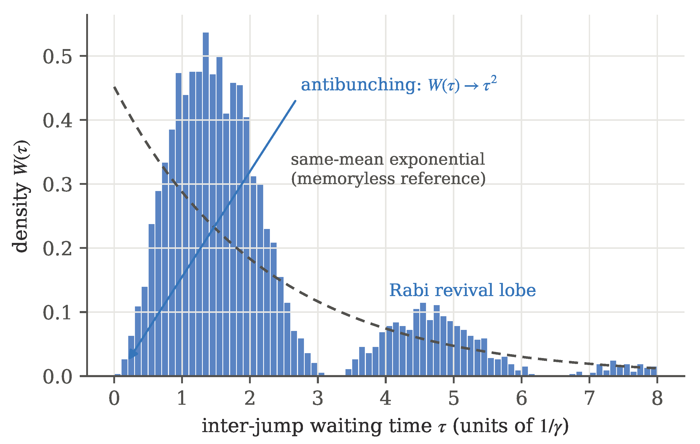
Figure 2.
Measured click rate versus non-paralyzable dead time (, , /point, error bars SE). The dashed curve is the exact finite-horizon delayed-renewal expectation computed from the no-jump survival (independent numpy implementation); every measured point sits within half-widths of it. The Poisson formula (dotted) under-predicts everywhere because antibunched arrivals avoid the dead window.
Figure 2.
Measured click rate versus non-paralyzable dead time (, , /point, error bars SE). The dashed curve is the exact finite-horizon delayed-renewal expectation computed from the no-jump survival (independent numpy implementation); every measured point sits within half-widths of it. The Poisson formula (dotted) under-predicts everywhere because antibunched arrivals avoid the dead window.
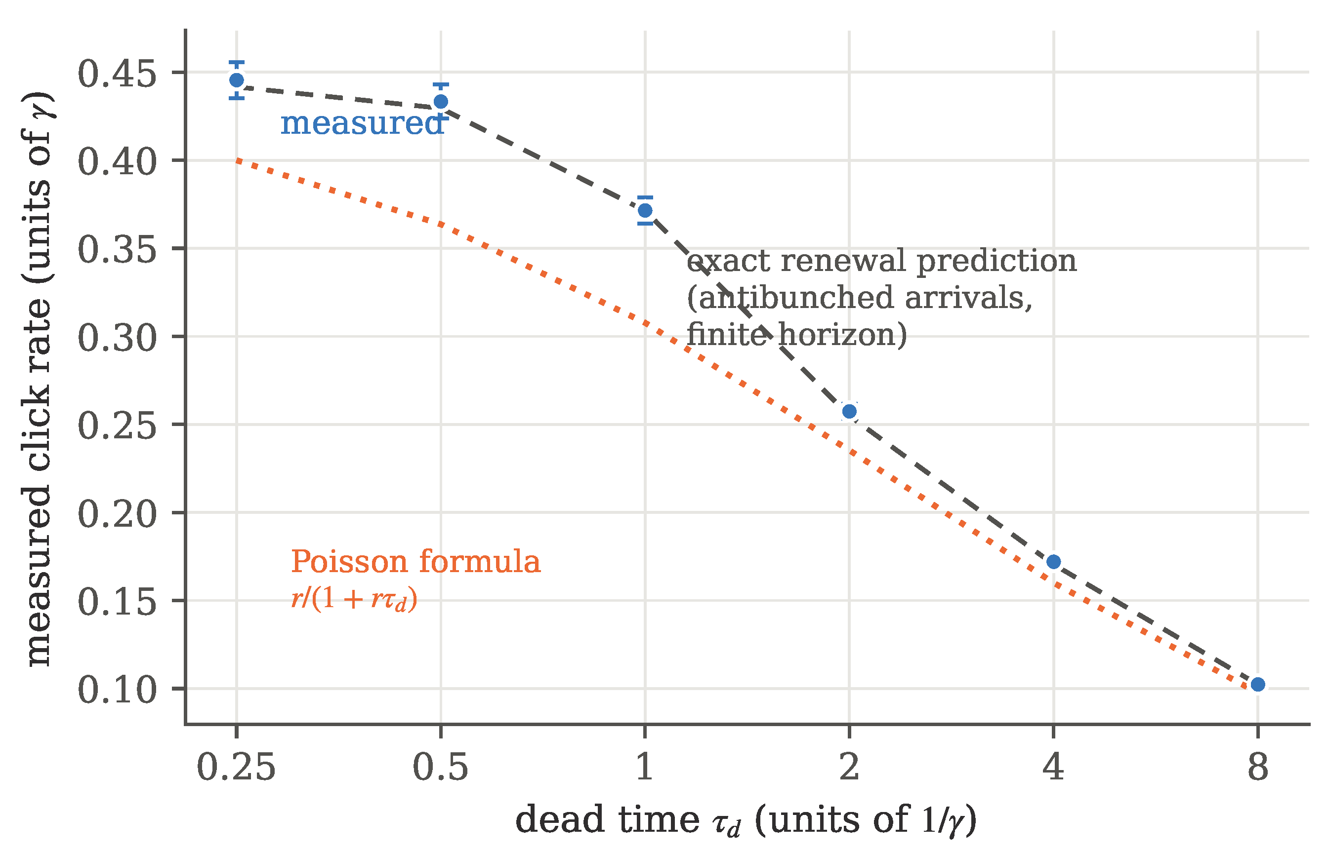
Figure 3.
(a) Variance ratio (unpaired over paired CI width, squared) for the estimated rate difference between two pulse-on-click protocols separated by latency gap (/arm). Pairing pays in proportion to trajectory alignment and approaches 1 as the protocols diverge. (b) The CRN audit’s ledger for the same comparisons: streams drawn by both arms (verified draw-identical) against each arm’s exclusive tail. The asymmetry is the signal: the slower variant’s exclusive set collapses toward zero while the baseline’s grows, because protocol distance manifests as one arm’s ordinal range outrunning the other’s. The audit is simultaneously the correctness check and the mechanism measurement.
Figure 3.
(a) Variance ratio (unpaired over paired CI width, squared) for the estimated rate difference between two pulse-on-click protocols separated by latency gap (/arm). Pairing pays in proportion to trajectory alignment and approaches 1 as the protocols diverge. (b) The CRN audit’s ledger for the same comparisons: streams drawn by both arms (verified draw-identical) against each arm’s exclusive tail. The asymmetry is the signal: the slower variant’s exclusive set collapses toward zero while the baseline’s grows, because protocol distance manifests as one arm’s ordinal range outrunning the other’s. The audit is simultaneously the correctness check and the mechanism measurement.
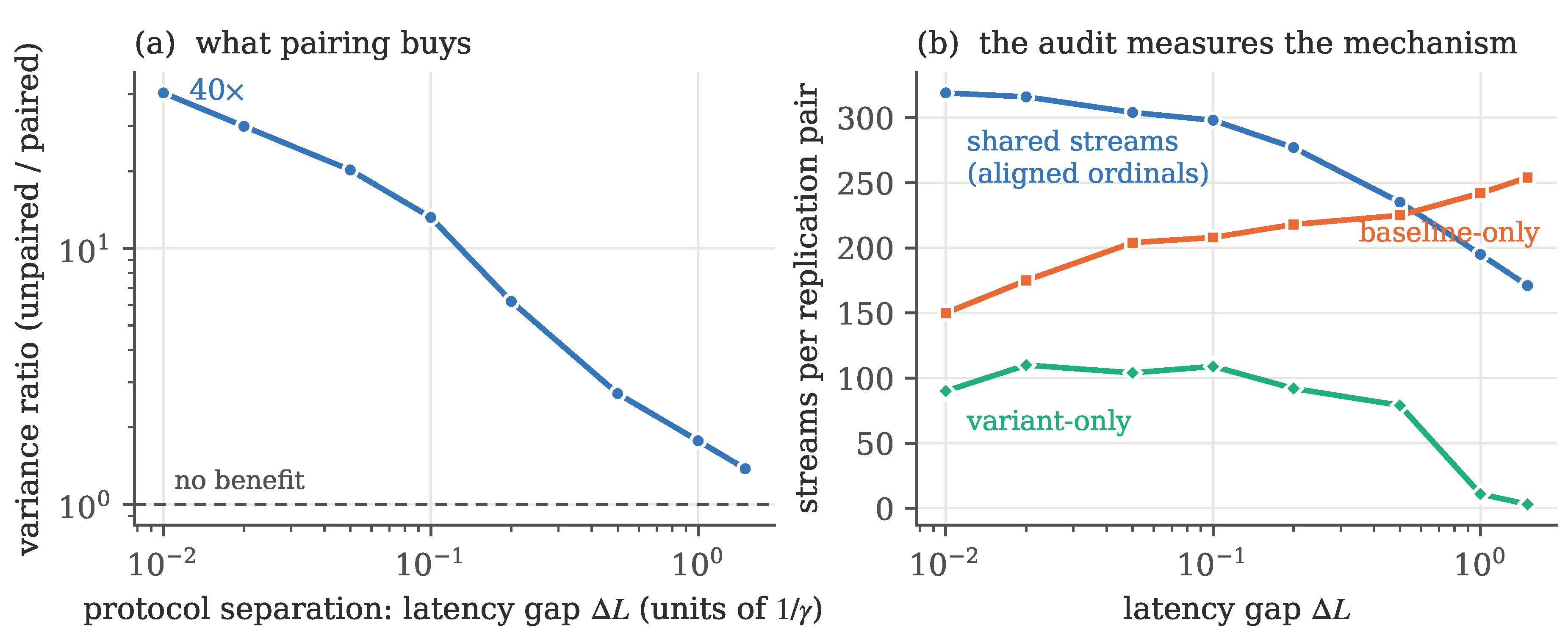
Figure 4.
(a) The rate-optimal pulse angle versus feedback latency at (dashed: renewal theory, independent numpy implementation). Measured points mark the paired baselines; the vertical bars span the two neighbor protocols, each resolved below its baseline at ( from Figure 5, the one-tick point from theta-zero.mjs, the rest from theta-L.mjs; baselines are the predicted optimum rounded to the grid of the sweep that produced them, for the theta-L and one-tick arms and at , where the baseline is against a prediction, with the neighbor protocols placed at from that baseline, and the leftmost point is plotted at the axis floor). The curve never reaches . (b) The zero-latency optimum versus drive strength: only as . The marker is this paper’s operating drive.
Figure 4.
(a) The rate-optimal pulse angle versus feedback latency at (dashed: renewal theory, independent numpy implementation). Measured points mark the paired baselines; the vertical bars span the two neighbor protocols, each resolved below its baseline at ( from Figure 5, the one-tick point from theta-zero.mjs, the rest from theta-L.mjs; baselines are the predicted optimum rounded to the grid of the sweep that produced them, for the theta-L and one-tick arms and at , where the baseline is against a prediction, with the neighbor protocols placed at from that baseline, and the leftmost point is plotted at the axis floor). The curve never reaches . (b) The zero-latency optimum versus drive strength: only as . The marker is this paper’s operating drive.
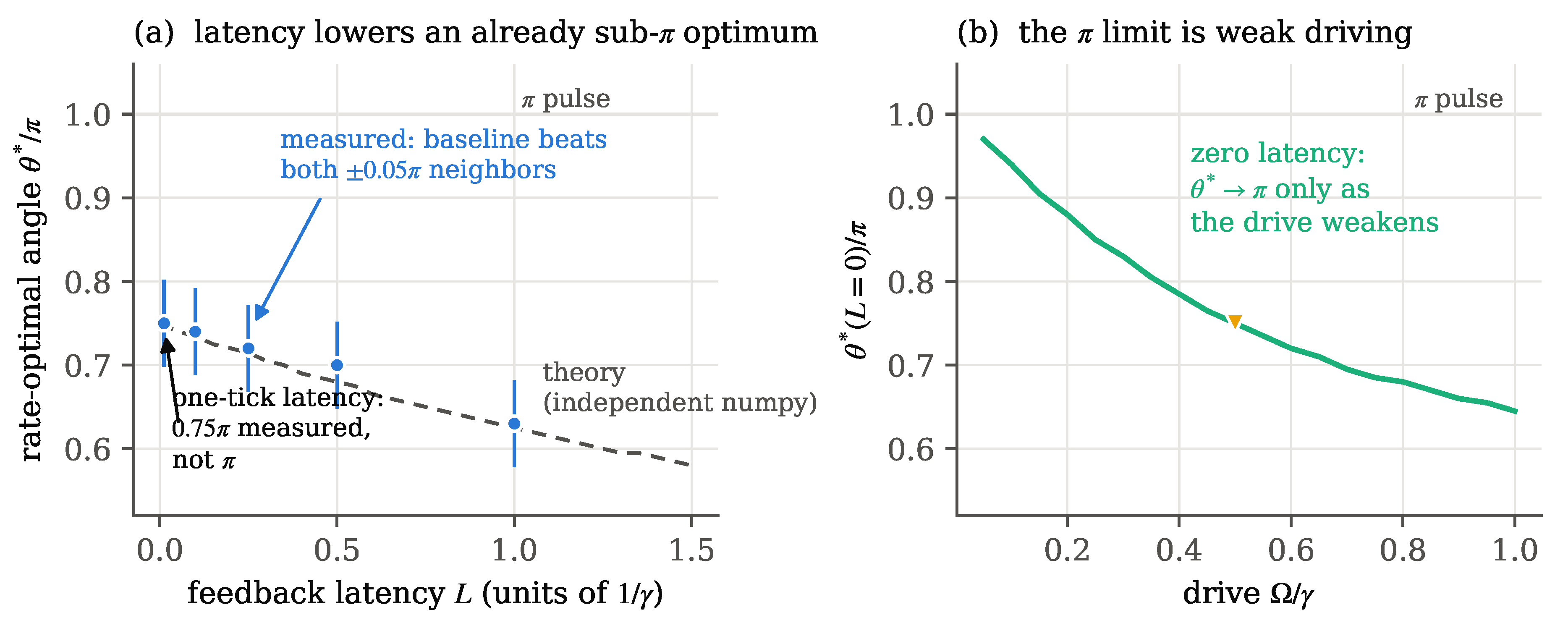
Figure 5.
(a) Click rate versus feedback pulse angle at , latency (/arm, error bars SE), against the exact finite-horizon renewal expectation (dashed; an independent numpy implementation). The optimum sits at , every measured point is within one half-width of the curve, and both declared neighbors are resolved below the optimum by the paired design. (b) Post-pulse excitation versus angle: the rate optimum (left line) is not the excitation optimum (right line). Coherence with the drive, not population, sets the re-emission clock.
Figure 5.
(a) Click rate versus feedback pulse angle at , latency (/arm, error bars SE), against the exact finite-horizon renewal expectation (dashed; an independent numpy implementation). The optimum sits at , every measured point is within one half-width of the curve, and both declared neighbors are resolved below the optimum by the paired design. (b) Post-pulse excitation versus angle: the rate optimum (left line) is not the excitation optimum (right line). Coherence with the drive, not population, sets the re-emission clock.
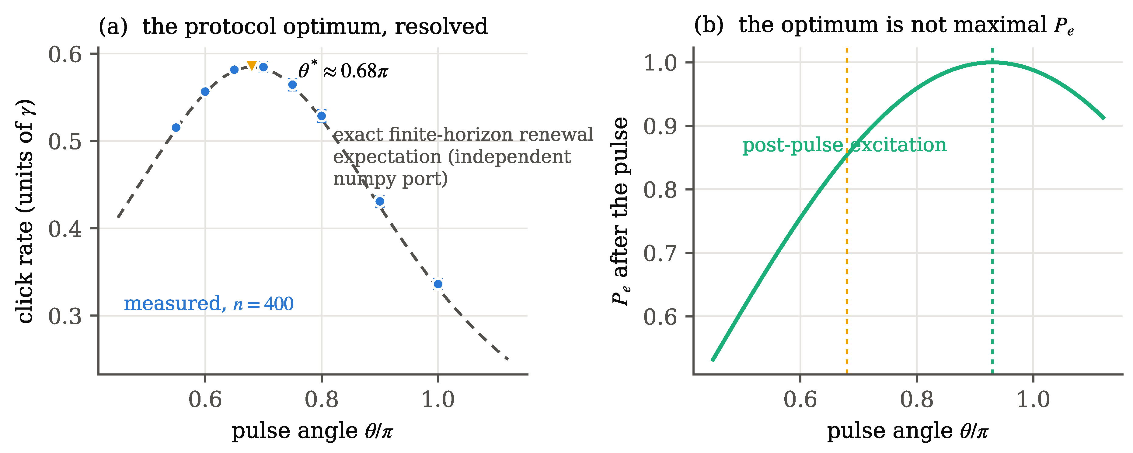
Figure 6.
The audit ledger as a predictor. Variance ratio against ledger overlap for all seventeen paired comparisons in this paper. Dashed: Eq. (6), fitted to the fourteen close-protocol comparisons only. The latency-gap and pulse-angle families lie on one line despite perturbing the interval density in different ways, one by translation and one by reshaping; calibrated on the eight latency comparisons alone, the relation predicts the six angle comparisons out of sample to a median factor of . The distant-protocol family sits off the line, in the regime Section 5.2 recommends running unpaired.
Figure 6.
The audit ledger as a predictor. Variance ratio against ledger overlap for all seventeen paired comparisons in this paper. Dashed: Eq. (6), fitted to the fourteen close-protocol comparisons only. The latency-gap and pulse-angle families lie on one line despite perturbing the interval density in different ways, one by translation and one by reshaping; calibrated on the eight latency comparisons alone, the relation predicts the six angle comparisons out of sample to a median factor of . The distant-protocol family sits off the line, in the regime Section 5.2 recommends running unpaired.
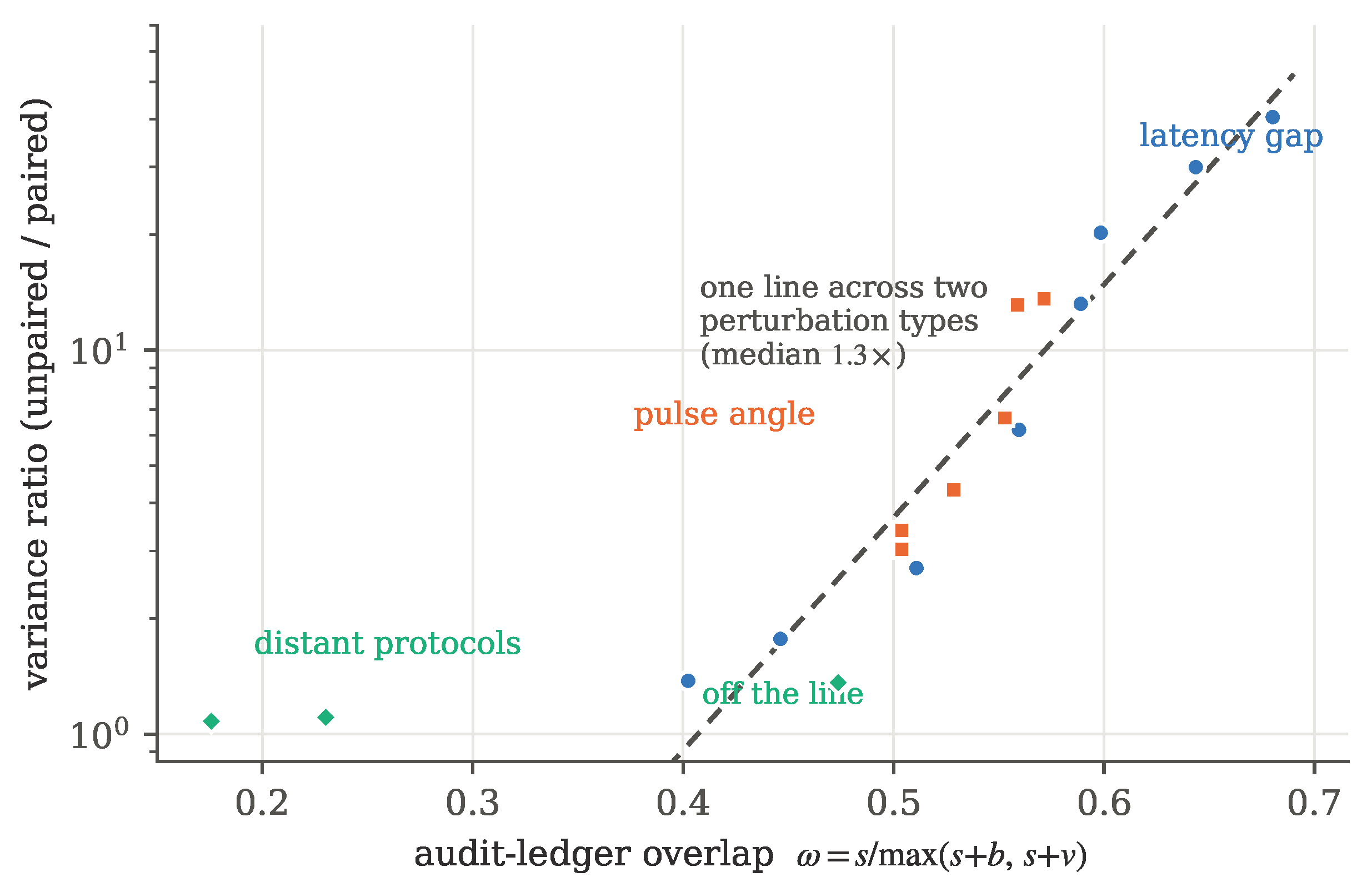

Table 1.
Known-answer gates (M0): the laboratory against the exact finite-horizon renewal expectation and the asymptotic steady state, , , , no dead time. The wait means (sampling error ) sit mildly below because the horizon censors the longest intervals; the rate column does not inherit that censoring. is the antibunching observable: the same-mean exponential reference would give 0.033 to 0.047 across these rows.
Table 1.
Known-answer gates (M0): the laboratory against the exact finite-horizon renewal expectation and the asymptotic steady state, , , , no dead time. The wait means (sampling error ) sit mildly below because the horizon censors the longest intervals; the rate column does not inherit that censoring. is the antibunching observable: the same-mean exponential reference would give 0.033 to 0.047 across these rows.
| rate (measured) | exact | R | wait | |||
|---|---|---|---|---|---|---|
| 0.3317 | 0.3333 | 2.984 | 3.000 | |||
| 0.4437 | 0.4444 | 2.252 | 2.250 | |||
| 0.4846 | 0.4848 | 2.069 | 2.063 |
Table 2.
The pulse-angle optimum against feedback latency at , from Eq. (4) (asymptotic cycle) and from the finite-horizon renewal sum at . The two differ by uniformly, inside the grid of the sweeps that placed the measured baselines.
Table 2.
The pulse-angle optimum against feedback latency at , from Eq. (4) (asymptotic cycle) and from the finite-horizon renewal sum at . The two differ by uniformly, inside the grid of the sweeps that placed the measured baselines.
| 0 | 0.1 | 0.25 | 0.5 | 1.0 | 1.5 | |
|---|---|---|---|---|---|---|
| , Eq. (4) | 0.750 | 0.735 | 0.713 | 0.680 | 0.624 | 0.581 |
| , finite horizon | 0.751 | 0.736 | 0.714 | 0.681 | 0.626 | 0.582 |
Table 3.
Estimators of the rate gap at , , decay times. The bound is the independent-arms Cramér-Rao floor; a coupled design is a strictly stronger experiment, so the bound constrains estimators that treat the two records separately and is not a limit on what coupling can achieve. Middle rows: idealized coupling.
Table 3.
Estimators of the rate gap at , , decay times. The bound is the independent-arms Cramér-Rao floor; a coupled design is a strictly stronger experiment, so the bound constrains estimators that treat the two records separately and is not a limit on what coupling can achieve. Middle rows: idealized coupling.
| estimator | SE at | ratio to floor | variance ratio |
|---|---|---|---|
| unpaired count (current practice) | 1.7% | 1 | |
| paired count, laboratory (Section 5.3) | 11% | 40 | |
| paired count, ideal coupling | 36% | 451 | |
| paired score, ideal coupling | 68% | 1598 | |
| information bound | 100% | 3433 |
Disclaimer/Publisher’s Note: The statements, opinions and data contained in all publications are solely those of the individual author(s) and contributor(s) and not of MDPI and/or the editor(s). MDPI and/or the editor(s) disclaim responsibility for any injury to people or property resulting from any ideas, methods, instructions or products referred to in the content. |
© 2026 by the authors. Licensee MDPI, Basel, Switzerland. This article is an open access article distributed under the terms and conditions of the Creative Commons Attribution (CC BY) license (http://creativecommons.org/licenses/by/4.0/).
Copyright: This open access article is published under a Creative Commons CC BY 4.0 license, which permit the free download, distribution, and reuse, provided that the author and preprint are cited in any reuse.