

Submitted:
28 August 2026
Posted:
31 August 2026
You are already at the latest version
Abstract
Spatial transcriptomics (ST) measures gene expression while retaining the location of each measurement in tissue. This makes it possible to study how molecular patterns relate to tissue structure, but it also creates data that depend on both gene expression and spatial relationships. Graph neural networks (GNNs) are increasingly used to model these relationships across tasks such as spatial domain identification, data integration, imputation, deconvolution, cell--cell communication analysis, and expression prediction. Yet methods with similar GNN architectures may represent different biological units, connect them using different evidence, and produce outputs with different biological meanings. This review provides a practical framework for comparing ST-GNN methods from input data to graph construction, graph-based learning, and downstream output. We focus on what each node represents, how relationships between nodes are defined, and how the graph contributes to the final output. Our analysis shows that node definition sets the resolution of the output, edge construction controls which relationships the model can use, and the role of the graph during learning determines how relational information contributes to the model output. This framework helps readers compare methods more consistently and assess what biological conclusions their outputs can support.
Keywords:
spatial transcriptomics
; graph neural networks
; graph construction
; graph learning
; spatial data analysis
1. Introduction
Bulk RNA sequencing averages gene expression across tissue, whereas dissociated single-cell RNA sequencing resolves cellular heterogeneity but removes the original spatial arrangement of cells. Spatial transcriptomics (ST) measures gene expression while retaining the location of each measurement within tissue, allowing molecular states to be analysed in relation to tissue structure [1,2]. This spatial information enables analyses of tissue layers, tumour microenvironments, developmental gradients, local niches, and candidate cell–cell interactions [2]. Broader reviews have described ST technologies and analytical workflows [3]. In ST data, the biological meaning and spatial resolution of each observation depend on how the tissue is measured and processed. Platform resolution, capture geometry, segmentation, binning, image registration, and reference mapping determine what each observation represents and which spatial relations can be analysed [4].
GNNs are well suited to ST because they operate on entities connected by explicit relations. In an ST-GNN, however, the graph is a modelling decision rather than a direct copy of the tissue. A node may represent a spot, segmented cell, subcellular region, image patch, gene, or reference-derived pseudo-cell. An edge may represent spatial proximity, expression similarity, morphological similarity, a biological prior, or a correspondence across slices or datasets. These alternatives change both the information available during learning and the meaning of the resulting output.
Recent reviews have classified ST-GNN and related deep learning methods by graph architecture, general methodology, data modality, or analytical task [5,6,7]. A broader review of GNNs for single-cell omics provides additional architectural and application context [8]. More recently, graph design has also been examined as an organising principle for deep learning-based multi-omics integration, with attention to node schema, edge semantics, interaction type, and graph context [9]. These classifications identify major model families, tasks, and graph design choices, but they do not by themselves show how measurement units become nodes, how evidence becomes edges, or how a constructed graph affects a specific prediction in spatial transcriptomics. Two methods can use the same GNN backbone while representing different entities, propagating information over different relations, and supporting different biological conclusions.
This review examines ST-GNN methods through the sequence shown in Figure 1: spatial inputs, graph construction, graph-based learning, and downstream applications. We separate five analytical components within this sequence: node definition, edge construction, graph structure, the use of the graph during learning, and the output produced for a downstream task. We use to denote a graph with node set V, edge set E, and node feature matrix X. This organisation makes it possible to compare methods according to the entities they model, the evidence encoded in their relations, the operations performed on those relations, and the resolution and form of their outputs.
The review covers 89 representative ST-GNN studies and uses the main text to explain recurring methodological patterns. Section 2 defines the measurement units and information sources available before graph construction. Section 3 compares node definitions, edge-construction rules, and basic and extended graph structures. Section 4 examines how constructed graphs control propagation, weighting, topology adaptation, reconstruction, and cross-source correspondence. Section 5 compares six downstream application categories and states the output and evaluation requirements of each category. Figure 2 provide method-level comparisons of inputs, graph construction, learning objectives, outputs, tasks, dataset scale, computational resources, and code availability. Section summarise the methodological gaps identified by these comparisons. Non-GNN methods are included only when they clarify a graph-design assumption or an evaluation setting.
2. Spatial Inputs and Information Sources
Before an ST-GNN graph is constructed, two types of inputs are already available: measurement units and information sources. In the spatial data input layer of Figure 1, measurement units refer to the technical units in which gene expression and spatial information are recorded after measurement or preprocessing. Information sources include spatial, molecular, histological, prior, and reference information that can support graph construction. This section introduces these inputs as the data layer that precedes graph construction. As shown in panel (A) of Figure 1, ST data are generated at one of three measurement resolutions—spot, single-cell, or subcellular. These resolutions determine what each graph node can represent in later stages.
2.1. Measurement Settings in Spatial Transcriptomics
Spatial transcriptomics (ST) measures gene expression in situ while preserving tissue context, providing information that is not available from dissociated single-cell profiles [1]. Previous reviews have summarised the development of spatial transcriptomics technologies and their analytical implications [2]. Other surveys have further discussed platform diversity and downstream analysis workflows [3]. ST platforms differ in how molecular signals are captured, localised, and assigned to analysis units [4]. Capture-based platforms typically measure gene expression at spatial locations [1]. High-resolution sequencing platforms can provide spatial bins or molecule-level coordinates that are later aggregated for analysis [10]. Imaging-based platforms, such as MERFISH [11] and seqFISH+ [12], localise transcripts at single-cell or subcellular resolution before segmentation or aggregation. These differences directly influence graph construction because graph models are built from the measurements provided by each platform rather than from an ideal biological representation.
2.2. ST Measurement Units
This subsection describes spots, bins, and segmented cells as the measurement units generated by ST platforms or preprocessing workflows. It focuses on what is measured or assigned before graph construction. How graph nodes are constructed and the biological entities they represent are discussed in Section 3.1.
A capture spot records transcripts collected at a spatial location and may contain signals from multiple cells, depending on the platform resolution, tissue density, and capture geometry [1]. A spatial bin aggregates molecular counts within a defined region when the original measurements are available at a finer spatial resolution than the analysis requires [10]. A segmented cell is obtained by assigning transcript locations to cell boundaries or cell centres, typically in imaging-based or high-resolution workflows [13]. Although it more closely represents an individual biological cell than a spot or bin, it is still produced through computational segmentation. Consequently, misassigned transcripts, inaccurate cell boundaries, or centroid errors may affect both the measured expression and spatial location [13].
2.3. Information Sources for Graph Construction
Edge evidence refers to information that supports an assumed relationship before it is represented in a graph. The relationship may later be encoded as an edge, an edge weight, a graph view, a link across information sources, or a higher-order structure. Five sources of evidence commonly appear in ST-GNN methods: spatial coordinates, molecular profiles, histological or morphological information, biological priors, and reference information. Hybrid and multimodal graphs typically combine several of these sources rather than introducing a separate category of evidence.
2.3.1. Spatial Coordinates and Local Proximity
Spatial coordinates indicate that nearby units may share tissue context, physical neighbourhoods, or local microenvironmental conditions. However, spatial proximity alone does not establish molecular similarity, long-range correspondence, ligand–receptor communication, or functional interactions. Identifying these relationships usually requires additional molecular information, biological priors, or external validation [14]. Spatial coordinates can be converted into graph topology using radius cutoffs, k-nearest neighbours, Delaunay triangulation, or alpha-complex construction. These graph construction choices are discussed in Section .
2.3.2. Molecular Profiles and Expression Similarity
Expression profiles can be used to estimate transcriptomic similarity between spots, bins, or cells, including units that are not immediate spatial neighbours. However, the resulting similarity estimates are sensitive to sparsity, dropout, normalisation, feature selection, batch effects, and platform-specific noise [15]. Similarity computed from the expression profiles of two nodes provides an estimate of their molecular relatedness, whereas spatial coordinates capture positional relatedness. These two roles should remain conceptually distinct until the method specifies how they are used in graph construction and learning.
2.3.3. Histology and Morphology
Paired histology images and morphological features provide information about tissue architecture, cellular morphology, and pathological structure [7]. They can complement spatial coordinates and expression profiles, but morphological similarity is not equivalent to similarity in gene expression. The reliability of histological information depends on staining quality, image resolution, registration, feature extraction, and whether the relevant transcriptional state is visible in tissue morphology [16]. Histology therefore serves as an auxiliary source of information whose relevance depends on the downstream task.
2.3.4. Biological Priors
Biological priors provide external knowledge about relationships among genes, cell types, pathways, and candidate communication events. In current ST-GNN methods, these priors most commonly take the form of ligand–receptor pairs or pathway annotations [17]. Regulatory and gene-level priors are less common. They appear mainly in recent multiview models, which combine multiple sources of information, or heterogeneous graph models, which include different types of nodes or relations, such as stKeep [18] and MAGNET [19]. We therefore regard gene regulatory networks and gene–gene relations as emerging extensions rather than widely used sources of information. Like other external resources, biological priors are curated and context dependent. They are not direct observations from an ST assay.
2.3.5. Reference Information
Reference information links ST measurements to external datasets or atlases. These references are most often single-cell RNA sequencing datasets that contain cell type labels, cell state annotations, or expression profiles [20]. They can support label transfer, deconvolution, alignment, and mapping, but they also introduce assumptions about the correspondence between the reference and target data [20]. Relevant states may be absent from the reference, altered by disease or development, or affected by differences between platforms. In these cases, the model may transfer the closest available annotation rather than the correct biological state. The construction of pseudo-nodes and links across information sources is discussed in Section 3.
The measurement units and information sources described above are inputs to graph construction, but they do not yet form a graph. They become part of the graph only after a method defines the nodes, converts the available information into relations, and represents these relations as edges, weights, views, links across sources, or higher-order structures.
3. Graph Construction
The measurement units and edge evidence defined above provide the inputs for graph construction. Graph construction begins when a method represents these inputs as nodes, edges, and other graph components, as shown in the graph construction block of Figure 1. This section discusses node construction, edge construction, basic and extended graph structures, and reporting practices. How the resulting graph is used in model learning is discussed in Section 4.
3.1. Node Definition and Granularity
A graph node is defined by the modelling process and is not necessarily identical to a measurement unit. In some methods, nodes directly correspond to platform outputs such as spots, bins, or segmented cells. Other methods introduce computational entities, including pseudo-spots, image patches, genes, cell types, morphological regions, and units obtained from reference data. The first question in graph construction is therefore what each node represents and at what biological or technical scale its features are defined.
Panel (B) of Figure 1 illustrates this distinction by showing measurement units as dark dots and the nodes constructed from them as coloured circles. The mapping between the two depends on the graph structure. A measured node may correspond to one measurement unit, a pseudo-node may be constructed from reference data, and a graph with multiple entity types may obtain each node type from a different source. The following subsections discuss these node types in turn.
3.1.1. Spot Nodes
In spot-level graphs, each capture location is represented as a node, usually with a processed expression vector as its features. Such a node represents a local mixture of cellular signals rather than an individually segmented cell. Unless the method introduces additional node types or increases the output resolution, its embeddings, clusters, and predictions remain defined at the spot level. GraphST [21] illustrates this basic setting. STAIG [22] uses the same spot-level nodes but changes how image information modifies the graph between spots.
3.1.2. Cell Nodes
In cell-level graphs, nodes represent segmented cells or cell-level observations, most often in imaging or spatial single-cell data. Because segmentation determines the node set, cell boundaries, centroids, and transcript assignments become part of graph construction rather than merely preprocessing details. CellNEST [23] and DeepTalk [24] illustrate this setting. Both define spatial or ligand–receptor-informed connections between cells, so the resulting neighbourhoods, interactions, and predictions differ fundamentally from spot-level outputs rather than simply providing a denser representation.
3.1.3. Pseudo-nodes and Nodes from Reference Data
Some deconvolution methods construct pseudo-spots from annotated single-cell reference data by mixing several cells and using their cell-type proportions as known labels. DSTG [25] connects these pseudo-spots with measured ST spots through expression similarity. STdGCN [26] further uses cell-type-aware sampling and separates an expression graph containing pseudo-spots and measured spots from a spatial graph containing only measured spots. These design choices determine how reference information is transferred to the spatial data.
3.1.4. Patch, Gene, and Multi-Entity Nodes
Some methods use node types that differ further from the original measurement units. Methods for image integration and super-resolution may introduce image patches, superpixels, or sub-spot units. For example, scstGCN [27] combines information from cells, spots, and image patches to infer expression at single-cell resolution from spot-level ST data.
Other methods introduce genes or several entity types into the graph. GCNG [28] represents genes as nodes. STING [29] constructs a gene co-expression graph for each spot and uses an inner GNN to encode it. The resulting spot representations are then connected in a second graph based on spatial proximity. HEIST [30] connects spatial cell–cell structure with gene or protein co-expression. stKeep [18] represents cells, genes, and histological regions in a heterogeneous graph. For these graphs, each node type and its source should be stated explicitly.
3.2. Edge Construction and Graph Structure
After the node set is defined, edge evidence is converted into edges or other graph components. Edges may be binary or weighted, directed or undirected, typed or untyped, and pairwise or higher order. A method may also preserve different information sources as separate graph views rather than merging them into a single adjacency matrix. The next question in graph construction is therefore how each source is represented in the graph.
The information source and the construction rule should be distinguished because the same source can produce different graph structures. Spatial coordinates may define a radius graph, a k-nearest-neighbour graph, a Delaunay graph, an alpha-complex graph, or an adjacency matrix weighted by distance. Expression profiles may define edges between molecularly similar nodes, assign weights to an existing spatial graph, or form a separate expression graph. Histology, biological priors, and reference information may also be represented through scalar weights, candidate edges, typed edges, links between sources, or auxiliary graph components. The construction rule should therefore be reported separately from the information source.
The edge panel in Figure 1(B) illustrates several resulting structures, including a single adjacency matrix, heterogeneous and virtual edges, weights defined by spatial distance or feature similarity, multiple graph views, and hyperedges. The following subsections discuss neighbourhood construction, weighted edges, and structures beyond a single adjacency matrix.
3.2.1. Neighbourhood Construction
Neighbourhood construction defines the candidate edge set using rules such as k-nearest neighbours, radius thresholds, Delaunay triangulation, or alpha-complex construction. Although these rules are often treated as routine preprocessing, each imposes a different assumption about local connectivity. A k-nearest-neighbour graph fixes the number of neighbours for each node. A radius graph instead uses a fixed physical distance. An alpha-complex graph uses spatial geometry to preserve local connectivity.
GraphST [21] and SEDR [31] construct k-nearest-neighbour graphs from spatial coordinates, although they use the resulting graphs in different learning systems. Other methods adopt different geometric rules. Novae [32] constructs a Delaunay graph, whereas SCAN-IT [33] uses an alpha complex. From the perspective of graph construction, these methods differ in which node pairs are connected before learning begins.
Neighbourhood construction is transparent and reproducible, but its parameters remain modelling choices. The radius threshold, number of neighbours, or geometric rule determines which local connections are available to the model. A later GNN may learn attention weights over these connections, but it can only reweight edges already included in the candidate set. Learned edge weighting is discussed in Section 4.2.
3.2.2. Weighted Edges
Weighted edge construction assigns scalar values to connected node pairs. The weights may reflect spatial distance, expression similarity, morphology, biological priors, or fixed combinations of several information sources. The key distinction is whether these weights are specified during graph construction or learned by the model.
SpaGCN [34] provides a clear example of weights specified before learning. It combines spatial distance with information extracted from histology images, so edge strength is determined before message passing. Spatial-ID [35] represents a less clear boundary case because it uses an adaptive weighted spatial graph. Nevertheless, these weights should be distinguished from attention weights or other edge weights learned during model training. Otherwise, fixed graph weights and learned weighting mechanisms may be incorrectly treated as the same design choice.
3.3. Basic Graph Structures
The node and edge choices described above can produce a basic graph structure with one dominant node type and one main adjacency matrix. In ST-GNNs, this is often a graph of spots or cells connected according to spatial proximity, expression similarity, or morphological information. A basic structure is not necessarily biologically simple. The node type, edge construction rule, and weighting scheme still determine which local connections are available to the model. The structure is considered basic because one main edge type connects one dominant set of nodes. It therefore provides a reference point for structures with multiple views, entity types, edge types, or information sources.
3.4. Extended Graph Structures
Some graph structures cannot be represented by a single adjacency matrix over one node type. They may preserve several edge sources as separate graph views, include multiple node or edge types, represent connections among groups of nodes, or link nodes across references, slices, samples, or modalities. These structures do more than add complexity to a basic graph. They allow the graph to represent different forms of biological and technical information.
3.4.1. Multiview Graphs
Multiview graphs preserve spatial proximity, expression similarity, histological similarity, or other edge sources as separate views rather than combining them into one adjacency matrix. Graph construction must therefore specify how each view is built, what information it represents, and whether the views remain separate during learning.
MuCoST [36] uses separate graphs for spatial proximity and expression correlation, whereas stMVC [37] uses separate spatial and histological similarity graphs. Because these relations are represented in different graphs, the model can process each information source separately. This differs from methods that merge spatial, molecular, and histological information into a single weighted adjacency matrix.
3.4.2. Heterogeneous and Hierarchical Graphs
Heterogeneous and hierarchical graphs contain multiple entity types, edge types, or graph levels. stKeep [18] connects cells, genes, and histological regions. STING [29] combines an outer spatial graph with inner gene–gene graphs. HEIST [30] connects spatial cell–cell structure with gene or protein co-expression. Unlike a basic graph of spots, these structures represent connections among different biological entities or across different scales. Each edge type therefore supports a different interpretation.
3.4.3. Hypergraphs
Hypergraphs represent connections among groups of nodes rather than only between node pairs. A hyperedge can connect several units that share a common higher-order pattern. HAST [38], for example, constructs local hypergraphs from gene expression, spatial information, and histology. It then aggregates them to represent many-to-many relationships among spots. In this setting, the basic connection unit changes from a pair of nodes to a group of nodes. This change affects how the resulting embeddings and clusters should be interpreted.
3.4.4. Links Across Sources
Links across sources connect nodes that do not belong to the same original spatial graph. In deconvolution, these links connect pseudo-nodes or reference profiles to measured spatial nodes, as in DSTG [25] and STdGCN [26]. In spatial integration, STAligner [39] uses mutual nearest neighbour anchors across slices. SLAT [40] aligns graphs from different slices through adversarial matching. Graspot [41] constructs probabilistic correspondences using optimal transport, while Tacos [42] combines graph structure with community and anchor information. In these methods, correspondence is explicitly constructed as part of the graph rather than inferred only from a single spatial neighbourhood.
3.5. Summary of Graph Construction Choices
Graph construction determines three properties of an ST-GNN: the entities represented by the model, the relations available for information exchange, and the organisation of those relations within the graph. Node definition sets the analytical unit and constrains the resolution of the resulting output. Edge construction specifies which spatial, molecular, histological, prior, or cross-source relations enter the model. Graph organisation determines whether these relations are merged into one adjacency structure, preserved as separate views or edge types, arranged across hierarchical levels, or represented as higher-order connections.
These construction choices are distinct from the role assigned to the graph during learning. The same constructed graph may define a message-passing neighbourhood, provide candidate relations for scoring, serve as a reconstruction target, support cross-source alignment, or impose a structural constraint. Conversely, similar learning operations may be applied to graphs that represent different entities and relations. Separating graph construction from graph usage therefore allows methods to be compared at both the representation and learning stages.
4. Constructed Graphs in Learning Systems
Panel (C) of Figure 1 shows how a constructed graph enters representation learning. The graph can define message passing, restrict candidate relations, provide structure for correspondence inference, or become a reconstruction target. Its role is determined by how the model uses it, not by the construction rule alone.
4.1. Roles of Constructed Graphs in Learning
In propagation models, the graph specifies which nodes exchange information. GraphST [21] uses a fixed spatial graph for GCN aggregation and reconstructs expression rather than spatial edges. In candidate-relation models, the graph restricts the relations that can be scored. CellNEST [23] builds directed communication candidates from spatial proximity and ligand–receptor expression, then ranks those candidates with attention. GCNG [28] has a different role: it builds a spatial cell graph for each candidate gene pair and performs graph-level binary classification, so the predicted unit is the gene pair rather than an edge in the spatial graph.
Constructed graphs can also provide structure for correspondence inference. SLAT [40] learns graph-informed representations within each slice and then matches cells or spots across slices. Graspot [41] learns graph-aware representations before estimating a soft transport plan with unbalanced optimal transport. Here the within-slice graph informs the matching problem but does not itself encode the cross-slice correspondence.
Some methods treat a graph as a target. DeepLinc [43] generates a cell–cell interaction adjacency from spatial single-cell expression data. The reconstructed graph can be reported directly or used as an auxiliary target that shapes the embedding.
4.2. Graph Structure during Learning
ST-GNNs differ in which parts of graph structure can change during training. SpaGCN [34] fixes a weighted adjacency from spatial distance and histology before optimisation. STAGATE [44] fixes the edge set but learns attention coefficients on those edges; non-neighbouring nodes in the initial graph never enter the attention calculation.
Other methods change the graph more directly. SGAE [45] first removes spatial edges that cross expression-based preclusters, then creates representation-dependent graph views through low-similarity edge removal and graph diffusion. asGNN [46] learns a stochastic subgraph through a variational information bottleneck, retaining or suppressing relations from a candidate spatial graph. STAGUE [47] jointly infers adjacency and node representations, allowing connections absent from the initial spatial graph. These examples separate fixed graph construction, learned edge weighting, candidate-edge selection, and broader topology inference.
Adaptive adjacency should also be separated from view fusion. STMGAMF [48] adapts node relations within spatial and feature graph branches, then fuses the resulting embeddings. The first operation changes propagation within a graph view; the second combines representations across views.
4.3. Graph Operators and Message Passing
Graph operators determine how information moves across constructed relations. Standard graph convolution aggregates over one adjacency matrix with a shared propagation rule. Graph attention changes neighbour contributions within the supplied edge set. Multiview and relational operators preserve information that a single adjacency would merge. Spatial-MGCN [49] encodes spatial and expression graphs separately before combining their representations. RGAST [50] represents communication at several spatial scales and applies relation-specific attention.
Other operators change the scope or geometry of propagation. SiGra [51] uses a graph transformer to integrate transcriptomic and image information. HGNN [52] constructs hyperedges from dense overlapping subgraphs and passes messages between nodes and hyperedges, so propagation occurs through node groups rather than only pairwise edges. MManiST [53] encodes the same graph in Euclidean, Poincaré, and Lorentz spaces before combining the representations.
4.4. Decoders, Prediction Heads, and Outputs
Outputs differ in unit, form, and resolution. SEDR [31] produces a spot embedding and reconstructs expression. Hist2ST [54] and THItoGene [55] predict expression from histology at the measured spot grid, whereas scstGCN [27] predicts expression below the measured resolution.
Pair-level outputs attach predictions to candidate pairs. GCNG [28] classifies candidate gene pairs, CellNEST [23] scores directed ligand–receptor candidates, and DeepTalk [24] predicts communication from subgraphs centred on candidate cell pairs. Graph-level outputs reconstruct relations instead of scoring a fixed candidate list. DeepLinc [43] reconstructs a cell–cell interaction network, and MAGNET [19] reconstructs several biological interaction graphs.
Composition outputs remain node-indexed but have a different interpretation. DSTG [25] and STdGCN [26] estimate a vector of cell-type proportions for each spot from reference-derived pseudo-spots. NicheCompass [56] reports cell- or spot-indexed niche representations and gene-programme activities that describe local microenvironments. These output types support different levels of biological interpretation, from spatial embeddings and expression estimates to candidate interactions, reconstructed networks, and reference-dependent composition estimates.
4.5. Training Objectives
Training objectives specify what the representation must recover, distinguish, match, regularise, or predict. Reconstruction losses target different objects: SEDR [31] reconstructs expression and graph structure, DeepLinc [43] reconstructs a cell–cell interaction network, and MAGNET [19] reconstructs several biological relation graphs.
Contrastive objectives depend on how related units or views are defined. CCST [57] contrasts nodes with context from a spatial neighbour graph. MuCoST [36] defines relatedness through spatial and expression views. conST [58], STAIG [22], Tacos [42], and SpaMask [59] use multimodal, augmented, community-aware, or masked views. HAST [38] uses hyperedges for group-wise message passing, but its contrastive positives are not defined by hyperedge membership alone.
Alignment and transfer objectives connect datasets or slices. STAligner [39] forms triplets from mutual nearest neighbours across slices. stGuide [60] uses reference annotations to organise the representation and transfer labels. Graspot [41] uses unbalanced optimal transport to estimate partial correspondence. Adversarial learning appears in stAA [61], where a discriminator separates graph-autoencoder codes from samples drawn from a prescribed prior and the encoder is trained to match the two distributions. Supervised objectives include reference-based label transfer in Spatial-ID [35] and reference-derived proportion prediction in DSTG [25].
4.6. Summary of Graphs in Learning Systems
The value of graph learning in spatial transcriptomics is not greater flexibility by default. It is the placement of graph flexibility where the biological uncertainty lies. When spatial proximity, histology, or ligand–receptor knowledge provides a reliable prior, the graph can constrain representation learning. When these priors are only proxies for communication, correspondence, or predictive dependence, the model needs mechanisms that revise edge weights, select candidate relations, or infer structure.
This distinction matters for edge-indexed outputs. Attention weights, interaction scores, reconstructed adjacencies, and adaptive predictive graphs all appear as edges, but they encode different quantities. The relevant question is where the graph departs from construction-time priors and whether that freedom matches the biological uncertainty of the ST task.
5. Downstream Applications
The preceding sections traced the process from ST inputs to graph construction and graph learning. This section turns to the application layer in Figure 1. It examines the outputs produced by ST-GNNs, the graph structures commonly used for different tasks, and the biological interpretations supported by these outputs.
The discussion is organised around six task categories. The broader categories of representation, relation inference, and mapping are used only to help orient the reader. Representative methods are included to show how downstream tasks are connected to choices in graph construction and learning.
The six task categories reviewed here focus on the primary outputs of ST-GNN methods. These outputs may also support subsequent analyses, including spatially variable gene detection, pathway enrichment, trajectory analysis, and the identification of disease-associated regions. Because these analyses are usually performed after embeddings, spatial domains, predicted expression, or aligned representations have been obtained, we do not treat them as separate task categories in this review.
5.1. Downstream Tasks, Outputs, and Graph Construction Patterns
This subsection groups ST-GNN applications according to their main downstream outputs. For each task category, we examine what the model produces, which graph structures are commonly used, and what biological interpretation the output can support. The categories are organised by analytical purpose rather than by GNN architecture, because similar operators may be used for different tasks, while the same task may be addressed using different graph structures and learning objectives.
5.1.1. Spatial Representation and Domain Identification
Methods for spatial representation and domain identification produce node embeddings, spatial domain labels, or both. Most assume that local spatial context is informative, but they incorporate this context in different ways. A spatial graph may define the message-passing neighbourhood or the candidate edges for attention. It may also provide a reconstruction target, define positive pairs for contrastive learning, be refined during training, or support the integration of multiple modalities. The task output alone therefore does not reveal the graph assumptions used to produce it. Methods for spatial domain identification illustrate this distinction. GraphST [21] uses a spatial graph in a self-supervised representation learning system. STAGATE [44] begins with a similar assumption about local neighbourhoods but learns different weights for candidate neighbours. Its outputs are therefore shaped by attention rather than uniform aggregation. SEDR [31] learns spatial representations through expression and graph reconstruction, whereas CCST [57] uses contrastive learning between nodes and their graph context. These methods may produce similar embeddings or domain labels, but they differ in what information the local graph is expected to preserve. These outputs mainly support the identification of spatially coherent groups, regional patterns, and node representations that incorporate local context. They do not by themselves establish biological tissue boundaries or cell-level mechanisms. Such claims require additional evidence from marker genes, histology, explicit boundary evaluation, perturbation experiments, or other biological validation. The comparison of recent methods in Section 5.2 develops this point further by showing that similar task labels and benchmark scores can conceal important differences in graph construction and graph usage.
5.1.2. Integration, Alignment, and Mapping
Methods for integration, alignment, and mapping produce aligned embeddings, correspondences across slices or samples, transferred labels, or mapped spatial structures. Unlike methods for domain identification, they do not focus only on whether spatial context is coherent within a single sample. They also identify which units across slices, samples, modalities, or references should correspond to one another. Graph construction must therefore preserve spatial organisation within each source while introducing links that support comparison across sources.
STAligner [39] combines within-slice spatial structure with anchors across slices to align comparable spatial contexts. SLAT [40] matches graph representations from different slices. Graspot [41] uses optimal transport to infer probabilistic correspondences rather than fixed one-to-one matches. Tacos [42] combines local graph representations with supervision from cross-slice anchors. The resulting correspondences are supported by the model rather than directly observed. Their interpretation depends on how anchors are defined, how well spatial structure is preserved within each source, and whether differences specific to individual samples remain detectable.
5.1.3. Cell–cell Communication and Niche Inference
Methods for cell–cell communication and niche inference produce two main types of output. Communication methods usually prioritise candidate interactions between cells or ligand–receptor pairs. Niche methods instead identify the microenvironmental state or programme associated with a cell or tissue region.
GCNG [28] and CellNEST [23] mainly score candidate interactions. DeepLinc [43] reconstructs an inferred interaction network, whereas NicheCompass [56] learns niche representations informed by biological priors. These outputs can support hypotheses about cellular interactions or descriptions of local microenvironments. However, they do not by themselves establish active signalling or downstream biological responses. Such claims require additional molecular, spatial, or perturbation evidence.
5.1.4. Imputation and Denoising
Methods for imputation and denoising produce reconstructed, denoised, or imputed expression values. These tasks are often grouped together because they all generate expression matrices. However, the meaning of a recovered value depends on the information available to the model and the assumptions used during recovery. The estimate may be informed by neighbouring nodes, generated by a probabilistic model, predicted from multiple modalities, or produced through a combination of these mechanisms.
Impeller [62] estimates missing or noisy expression using spatial context and similarities between expression profiles. stMCDI [63] instead uses masked conditional diffusion. Its imputed values are generated under spatial and gene correlation constraints rather than obtained only by averaging nearby observations. SiGra [51] combines transcriptomic and histological information through multimodal graph learning, so its recovered expression may reflect both molecular neighbourhoods and image context.
These methods may produce similar denoised expression matrices despite relying on different recovery assumptions. Imputed or denoised expression should therefore be interpreted as an estimate produced by a specific graph and learning system, not as directly recovered ground truth. Stronger validation requires held-out genes or locations, independent measurements, biological replicates, or estimates of prediction uncertainty.
5.1.5. Deconvolution
Deconvolution methods estimate cell type proportions or related measures of cellular composition for spatial units. Here, the graph is used mainly to transfer information from a labelled reference dataset to spatial measurements rather than to identify local tissue domains. The resulting estimates therefore depend on the reference data, including their cell type coverage, similarity to the spatial sample, and the procedure used to connect the two sources. Spatial context may further influence the estimated composition.
DSTG [25] makes this transfer process explicit. It constructs pseudo-spots from single-cell reference data and uses them to infer cell type composition in measured spatial spots. STdGCN [26] distinguishes expression links between reference pseudo-spots and spatial spots from spatial links among measured spots. Its estimates therefore reflect both similarity to the reference and local spatial context. GTAD [64] also transfers information between single-cell reference data and spatial measurements through a graph.
Across these methods, the graph helps incorporate reference information into spatial analysis, but it does not remove dependence on the reference. Claims about tissue composition should therefore be supported by checks of reference coverage and comparability between the reference and target samples. Tests with alternative references and independent validation of cell types or spatial distributions can provide further support.
5.1.6. Expression Prediction from Histology and Super-Resolution
Methods for expression prediction from histology and super-resolution produce predicted expression maps, estimates at finer spatial resolution, or values for sub-spot locations. Unlike conventional denoising, these methods often predict beyond the locations or resolution directly measured by the transcriptomic assay. They combine morphology, spatial context, and observed expression, but their outputs remain predictions for unmeasured locations or spatial scales.
Hist2ST [54] uses image patch representations and local spatial dependencies to predict gene expression from histology. Its output is therefore an expression estimate conditioned on tissue morphology. THItoGene [55] follows a similar approach by learning representations from images and graphs to predict gene expression. scstGCN [27] extends this setting by combining several data sources to infer expression at single-cell resolution from spot-level measurements.
These methods can generate informative expression maps, but predicted expression should remain distinct from directly observed expression. This distinction is especially important when predictions are made below the native resolution of the assay. Stronger evidence may come from validation on held-out spatial locations, comparison with higher-resolution measurements, analysis of errors for individual genes, and uncertainty estimates for unmeasured locations.
5.2. Spatial Domain Identification as a Comparison Case
Spatial domain identification shows why benchmark scores should be read together with graph construction and learning choices. SpaMask, STAIG, STMGAMF, DACN, and stGCL are all evaluated on DLPFC benchmarks and report ARI or NMI against annotated cortical layers. Their outputs and metrics look comparable, but their graph designs differ. SpaMask masks nodes and edges during self-supervised learning. DACN combines a graph branch with an autoencoder. stGCL propagates expression and histology through graph attention and combines reconstruction with contrastive learning. STAIG perturbs edges using histology images. STMGAMF uses separate spatial and expression graphs and learns how to combine them.
ARI and NMI measure agreement with annotated domains, but they do not identify which model component produced the improvement. The reported DLPFC results also use different aggregation rules. SpaMask reports a median ARI of 0.596 across 12 slices. STAIG reports a median ARI of 0.69 and a median NMI of 0.71. STMGAMF reports a median ARI of 0.61 and a median NMI of 0.68. stGCL reports a mean ARI of 0.56 and a mean NMI of 0.65. DACN is not directly comparable because its main text presents boxplots and significance tests across 12 DLPFC sections, while reporting a slice-level ARI of 0.67 for section 151674. These values are useful evidence, but not a unified leaderboard.

Table 1.
Graph construction and graph usage in methods for spatial domain identification evaluated on DLPFC benchmarks. Methods with similar task outputs and clustering metrics may use different graph structures, learning roles, and model components.
Table 1.
Graph construction and graph usage in methods for spatial domain identification evaluated on DLPFC benchmarks. Methods with similar task outputs and clustering metrics may use different graph structures, learning roles, and model components.
| Method | Graph construction | Graph usage during learning | Component not reflected by the score |
| SpaMask [59] | Spatial graph constructed from spot coordinates | Masked nodes are used for feature reconstruction, while masked edges are used for contrastive learning within a shared encoder | Node and edge masking |
| STAIG [22] | Spatial graph whose edges are perturbed using histology images | Representations from perturbed graphs are compared through contrastive learning between neighbouring spots | Edge perturbation using histology |
| STMGAMF [48] | Separate spatial and expression graphs, with edge weights learned during training | The two graphs are encoded separately and then combined under reconstruction and spatial regularisation objectives | Individual graph views and loss terms |
| DACN [65] | Spatial graph constructed from spot coordinates | The graph encodes expression representations produced by an autoencoder, and the two branches are combined for reconstruction | Autoencoder and graph branches |
| stGCL [66] | Spatial graph containing expression and histology features | The graph propagates both modalities, reconstructs each modality, and supports contrastive learning | Contribution of histology |
Transfer to other datasets depends on the available modalities and modelling assumptions. A method that benefits from histology on DLPFC may lose that advantage when images are unavailable or differ in quality. STAIG uses histology to guide edge perturbation, and stGCL reports lower performance when its histology encoder is removed. Component-level comparisons are therefore needed to separate graph construction, graph usage, training objectives, modality availability, and clustering procedures.
5.3. Summary of Downstream Outputs and Validation
Across the six downstream task categories, the reviewed methods fall into three broader analytical modes according to what their outputs represent: representation and recovery, relational inference, and mapping and transfer across sources. This grouping does not replace the task taxonomy above. It connects each output type to the biological conclusion it can support and to the evidence relevant to evaluating that conclusion. Representation and recovery methods produce embeddings, labels, or expression estimates. Relational-inference methods produce candidate interactions, inferred networks, or summaries of local microenvironments. Mapping and transfer methods produce correspondences, transferred annotations, or composition estimates across slices, samples, modalities, or reference datasets. Table 2 states the role of the graph, the model output, the supported conclusion, and the corresponding validation evidence for each analytical mode.
Benchmark metrics assess specific properties of model outputs, while broader biological conclusions benefit from additional forms of validation. DLPFC spatial-domain benchmarks test clustering agreement and spatial representation, but they do not evaluate communication inference, deconvolution, cross-dataset integration, imputation, or histology-based expression prediction [67]. Benchmark design and platform characteristics can change reported method rankings [68,69]. Boundary and marker-gene evidence strengthen spatial-domain results. Held-out genes or locations test imputation results. Signalling evidence not used to construct candidate interactions strengthens communication results. Sensitivity analyses across references assess deconvolution results. Matched measurements at the target resolution provide direct validation for super-resolution results.
6. Future Directions
Future work can build on four priorities identified in this review. These are testing graph assumptions, developing evaluation for specific tasks, improving scalability, and representing a broader range of biological connections.
6.1. Testing Graph Assumptions
Graph construction should be evaluated as part of the model rather than treated as fixed preprocessing. Useful controls include removing individual edge sources, shuffling biological priors, changing neighbourhood rules, subsampling reference data, and testing alternative links across datasets. For example, methods for cell–cell communication can be tested with shuffled or held-out ligand–receptor pairs, while integration methods can be evaluated under different anchor rules. Representation methods can be tested across different neighbourhood sizes, distance thresholds, and spatial topologies.
These experiments can reveal whether performance is robust or depends strongly on one graph assumption. Future studies should also report the node type, edge information, construction rule, weighting scheme, retained graph views, links across sources, and the role of the graph during learning. This would make it easier to separate the effects of graph construction, GNN operations, output modules, and training objectives.
6.2. Task-specific Benchmarks and Validation
Evaluation should reflect the output and interpretation of each task. Spatial representation requires more than clustering agreement and can include boundary quality, marker support, agreement with histology, and sensitivity to graph parameters. Communication and niche inference require validation independent of the priors used to define candidate interactions. Integration should assess both correspondence across datasets and preservation of biological structure. Deconvolution and expression prediction should test reference robustness, resolution limits, and uncertainty.
DLPFC and similar benchmarks are useful for spatial domain identification, but they should not serve as general benchmarks for all ST-GNN applications. Broader benchmark suites should use separate evaluation criteria for integration, communication and niche inference, imputation, deconvolution, and expression prediction from histology. They should also distinguish the quality of the primary model output from the reliability of any later biological analysis built on that output.
6.3. Scaling Graph Systems
The methods summarised in our comparison table range from a few hundred spots to millions of cells, but computational information is reported unevenly. Future work should report graph size, hardware, runtime, memory use, and any sampling or approximation used during training and inference.
These choices can also change the biological information available to the model. Subgraph training, sparsification, approximate neighbour search, and partitioning may remove rare cell states, sharp boundaries, weak interactions, or distant correspondences. Their effects should therefore be evaluated rather than treated only as implementation details. Novae [32], for example, uses dynamically generated local subgraphs and lazy loading to operate on millions of cells. Such strategies improve efficiency, but they also determine which local structures are presented to the model.
Systems with several entity types create an additional challenge. HEIST [30] jointly models spatial connections among cells and co-expression among genes or proteins. Similar systems may combine spots, cells, genes, image patches, reference units, or tissue regions. Each node type, edge type, and output scale should be stated explicitly. The contribution of additional modalities should also be tested separately to determine whether they add independent information or mainly repeat spatial structure already present in other inputs.
Graph learning may also enter earlier stages of the pipeline. Segger [70], for example, uses graph learning during segmentation and therefore affects which cells later become graph nodes. This dependency should be made explicit because errors in node definition can propagate through all later stages.
6.4. Expanding Biological Connections
Future models may include regulatory links, pathway dependencies, cell state transitions, physical contacts, extracellular matrix interactions, paracrine gradients, and causal links supported by perturbation experiments. These connections should not be treated as interchangeable edges because they represent different biological mechanisms and support different claims.
Regulatory and gene-level priors are still less common than ligand–receptor pairs and pathway annotations. Future methods may incorporate gene regulatory networks, protein interactions, perturbation data, literature knowledge, or clinical information. Each source should be assigned a clear role in the graph. It may define candidate edges, assign edge weights, provide node features, guide supervision, or serve as validation evidence.
The main challenge is not simply to build larger or more complex graphs. It is to represent richer biological connections while keeping their meaning, scale, source, and validation requirements explicit.
7. Conclusions
This review organised ST-GNN methods as a sequence from spatial inputs and graph construction to graph-based learning and downstream applications. This view shows that methods with similar neural architectures can encode different analytical assumptions because they define different nodes, relations, graph structures, learning roles, and outputs. The graph should therefore be examined as part of the model specification rather than treated as a neutral preprocessing step.
Across application areas, the suitability of an ST-GNN method depends on whether its graph representation matches the biological scale, relation, and prediction required by the task. Comparisons based only on model architecture or aggregate performance obscure these differences. A component-level description of the input, graph, learning process, output, and evaluation provides a clearer basis for comparing methods and interpreting their results.
Table 3.
Method-level catalogue of GNN methods for spatial transcriptomics. Each entry summarises the main task, data type, additional inputs, graph construction, GNN backbone, approximate data scale, computational scale, and code availability. Scale records quantities stated in the original study, including numbers of samples, slices, spots, cells, or genes. Computational scale records explicitly stated hardware, runtime, memory use, or strategies for processing larger graphs. Only information reported in the original study is shown.
Table 3.
Method-level catalogue of GNN methods for spatial transcriptomics. Each entry summarises the main task, data type, additional inputs, graph construction, GNN backbone, approximate data scale, computational scale, and code availability. Scale records quantities stated in the original study, including numbers of samples, slices, spots, cells, or genes. Computational scale records explicitly stated hardware, runtime, memory use, or strategies for processing larger graphs. Only information reported in the original study is shown.
| Method | Year | Main task | Data | Additional input | Graph construction | GNN backbone | Scale | Computational scale | Code |
| GCNG | 2020 | cell-cell communication inference | seqFISH+; MERFISH | - | Spatial radius | GCN | 913 cells; 2,050 cells across 7 fields of view; 1,368 cells; 10,000 genes | url [28] | |
| SpaGCN | 2021 | spatial domain identification; spatially variable gene detection | ST; 10x Visium; Slide-seqV2; STARmap; MERFISH | optional histology | Histology-weighted spatial | GCN | 224 spots; 12 tissue slices; 3,353 spots; 16,448 genes | single Intel Core i5-8259U CPU @ 2.30 GHz; 16 GB memory; For mouse posterior brain data, SpaGCN completed spatial domain and SVG detection in less than 1 min,required 1.3 GB memory | url [34] |
| DSTG | 2021 | deconvolution | 10x Visium; Slide-seqV2; ST | scRNA-seq reference; pseudo-ST | Canonical correlation analysis/mutual nearest neighbor similarity | GCN | 2–8 cells per pseudo-spot; 500–4,000 spots; 5,000–50,000 reads per cell; 2,000 variable genes | url [25] | |
| SCAN-IT | 2021 | spatial domain identification | osmFISH; seqFISH; seqFISH+; Visium; Slide-seq | - | Alpha-complex spatial | GCN | 5,328 cells; 1,597 cells; 523 cells; 33 genes | url [33] | |
| STAGATE | 2022 | spatial domain identification | 10x Visium; Slide-seq; Slide-seqV2; Stereo-seq | - | Spatial neighbor; optional pruning | GAT | 12 sections; 3498–4789 spots per section; 19,109 spots; 3000 highly variable genes | Largest real dataset with >50k spots, approx. 40 min; simulated dataset with 50k spots, less than 40 min, approx. 4 GB GPU memory; local subgraphs or mini-batches | url [44] |
| CCST | 2022 | spatial domain identification; cell clustering | MERFISH; seqFISH+; 10x Visium | - | Hybrid spatial adjacency | GCN | url [57] | ||
| SpaceFlow | 2022 | Representation; spatial domain identification; pseudo-space map | 10x Visium; Stereo-seq; Slide-seqV2; seqFISH | - | Spatial-expression graph | GCN | 12 sections; 18,197 cells; 12 tissue sections; 28,243 genes | GeForce RTX 2080 Ti GPU; ST data with fewer than 10,000 cells, less than 5 min on GPU; 3,000–50,000 cells/spots, 30 s to 3 min on GeForce RTX 2080 Ti GPU | url [71] |
| conST | 2022 | Representation; spatial domain identification | MERFISH; seqFISH; 10x Visium; Stereo-seq | optional histology | Spatial kNN | GCN | 12 slices | url [58] | |
| DeepLinc | 2022 | cell-cell communication inference | seqFISH; MERFISH; HDST | - | Spatial kNN | GCN | 1,597 cells; 4,975 cells; 125 genes | url [43] | |
| stMVC | 2022 | spatial domain identification; tumor heterogeneity | 10x Visium; STARmap | Histology; region segmentation | Multi-view histology-similarity graph; spatial-location graph | GAT | 12 slices; 3460–4789 spots per slice; 3844 spots; 2000 highly variable genes | 20K spots, 38 min; local subgraphs or mini-batches, sampling | url [37] |
| Hist2ST | 2022 | histology-to-expression prediction | ST; 10x Visium; Space-TREX; Stereo-seq | Histology patches | Spatial kNN | GraphSAGE | 32 sections from 7 patients; 9612 spots; 12 sections from 4 patients; 785 genes | Ubuntu 18.04.7 LTS, Intel Core i7-8700K CPU @ 3.70 GHz, 256 GB memory | url [54] |
| SD2 | 2022 | deconvolution | seqFISH+; MERFISH; 10x Visium; ST | scRNA-seq reference | Transcriptional similarity; spatial | GCN | 523 cells; 6 cell; 2, 4.5 and 15.7 cells per spot; 135 genes | url [72] | |
| DeepST | 2022 | spatial domain identification; integration | 10x Visium; Slide-seqV2; Stereo-seq; MERFISH; 4i; MIBI-TOF | optional histology; molecular features | Spatial kNN; expression/morphology features | GNN | 12 slides; 10 cell; 3 consecutive imaging-based molecular slides; 33,538 genes | approx. 4000 spots and 30,000 genes, approx. 7 min on GPU, approx. 6G memory | url [73] |
| Spatial-ID | 2022 | cell type annotation; label transfer | MERFISH; Slide-seq; CosMx SMI; Stereo-seq | scRNA-seq reference labels | Distance-weighted Spatial neighbor | GCN | 12 samples; 280,186 cells; 159,738 cells; 254 genes | Workstation with 40 GB RAM, 10 cores of 2.5 GHz Intel Xeon Platinum 8255C CPU, Nvidia Tesla T4 GPU with 8 GB memory; Mouse spermatogenesis, average time cost per sample, 5.0 min | url [35] |
| NCEM | 2022 | cell-cell communication inference | MERFISH; CODEX; MIBI-TOF; MELC; chip cytometry; 10x Visium | cell-type labels; spot deconvolution | Radius-based spatial cell or spot graph | GNN | 40,864 WT cells; 284,098 cells; 11,321 cells; 132 genes | url [74] | |
| GraphST | 2023 | spatial domain identification; integration; deconvolution | 10x Visium; Stereo-seq; Slide-seqV2 | optional scRNA-seq reference | Spatial neighborhood | GCN | 12 slices; 3639 spots; 78,886 cells; 33,538 genes | Intel Core i7-8665U CPU, NVIDIA RTX A6000 GPU; E14.5 mouse embryo, approx. 100,000 spots, 30 min wall-clock time | url [21] |
| HoloNet | 2023 | cell-cell communication inference; functional cell effect decoding | 10x Visium; Slide-seqV2 | cell-type labels; ligand–receptor prior | Directed ligand–receptor multi-view | Attention GNN | 2, 5000 spots; 586 highly variable genes | url [75] | |
| STAligner | 2023 | integration; spatial domain identification | 10x Visium; Stereo-seq; Slide-seqV2; Slide-seq | multiple slices | Spatial neighbor; triplet-based cross-slice alignment | GAT | 4 adjacent DLPFC slices; 12 DLPFC slices; 4 mouse embryo slices | Runs on GPU or CPU; GPU is recommended | url [39] |
| SLAT | 2023 | integration | 10x Visium; MERFISH; Stereo-seq; seqFISH; Xenium; spatial-ATAC-seq | multi-omics; multiple slices | Per-slice spatial kNN | GCN | 3000 spots; 6500 cells; 100,000 cells; 20,000 genes | 16 cores of Intel Xeon Platinum 8358 CPU, 128 GB RAM, NVIDIA A100 GPU with 80 GB VRAM; Slices with over 100,000 cells each, 3 min | url [40] |
| STGNNks | 2023 | spatial domain identification; cell clustering | 10x Visium | - | Hybrid spatial adjacency | GCN | url [76] | ||
| SCGDL | 2023 | spatial domain identification | 10x Visium; Slide-seqV2 | - | Spatial neighbor | Gated GCN | 12 samples; 3798 spots; 150,392 reads per spot; 3000 highly variable genes | Ubuntu 20.04.5 LTS, Intel Core i9-12900F CPU @ 2.40 GHz, 64 GB memory, GeForce RTX 3090Ti GPU | url [77] |
| SiGra | 2023 | spatial domain identification; expression enhancement | CosMx SMI; MERSCOPE; 10x Visium | multichannel images | Spatial proximity cell/spot | Graph Transformer | 83,621 cells; 395,215 cells; 12 slices; 982 genes | url [51] | |
| Spatial-MGCN | 2023 | spatial domain identification; gene imputation | 10x Visium; Stereo-seq | - | Expression kNN; spatial radius | GCN | 3460–4789 spots; 12 slices; 19,109 spots; 33,538 genes | url [49] | |
| ConSpaS | 2023 | spatial domain identification; denoising | 10x Visium; Stereo-seq; Slide-seqV2 | - | Spatial neighbor; radius/kNN | GCN | 12 slices | url [78] | |
| spaCI | 2023 | cell-cell communication inference | seqFISH+; CosMx SMI; MERSCOPE | candidate ligand–receptor pairs | Spatial kNN; adaptive edge attention | Attention GNN | 523 cells; 81,236 cells; 18 cell; 10,000 genes | url [79] | |
| CGCom | 2023 | cell-cell communication inference | seqFISH | cell-type labels; ligand–receptor/downstream prior | Directed spatial threshold | GAT | 17,806 cells; 14,185 cells; 20,577 cells; 29,452 genes | url [80] | |
| SEDR | 2024 | Representation; spatial domain identification; integration | 10x Visium; Stereo-seq; Slide-seqV2 | - | Spatial kNN over spots/cells | GCN | 12 sections; 3460–4789 spots per section; 3493 spots; 27,106 genes | url [31] | |
| SSGCN | 2024 | spatial domain identification | 10x Visium; Stereo-seq; Slide-seqV2 | - | Spatial kNN with expression similarity edge reweighting | GCN | 2,695 spots; 3,798 spots; 21,724 cells; 3,000 highly variable genes | Intel Xeon Gold 5220 CPU at 2.20 GHz; approx. 1 min for each Visium dataset and approx. 8 min for each high-resolution mouse olfactory bulb dataset | - [81] |
| SGCAST | 2024 | spatial domain identification | 10x Visium; Stereo-seq; Seq-scope | - | Mini-batch expression; spatial proximity | GCN | 12 slides; 28,399 spots; 51,335 spots | Datasets with 3k–121k spots, 0.25 GB GPU memory; all datasets, less than 20 min; local subgraphs or mini-batches | url [82] |
| SpaGCAC | 2024 | spatial domain identification | 10x Visium; STARmap; Stereo-seq | - | Spatial kNN with adaptive self-loop | GCN | url [83] | ||
| SGAE | 2024 | spatial domain identification | 10x Visium; seqFISH; MERFISH; Slide-seqV2; Stereo-seq | - | Spatial kNN; type-aware pruning; distortion | GNN | 12 continuous slides; 19,416 cells; 3,106 cells; 351 genes | url [45] | |
| stAA | 2024 | spatial domain identification | 10x Visium; Slide-seqV2; Stereo-seq; STARmap | - | Spatial neighbor | GCN | 12 slices; 3460–4789 spots per slice; 3798 spots; 10,725–21,897 genes | url [61] | |
| stMMR | 2024 | spatial domain identification | 10x Visium; ST; NanoString CosMx SMI | Histology | Weighted spatial | GCN | 12 sections; 8 major cell; 4 slices | url [84] | |
| stImpute | 2024 | imputation | STARmap; osmFISH; MERFISH; Xenium; paired scRNA-seq references | scRNA-seq reference; ESM-2 embeddings | ESM-2 protein-similarity gene graph | GraphSAGE | 1549 spatial cells; 14,249 cells; 3405 spatial cells; 1020 genes | Ubuntu 18.04.7 LTS, Intel Core i7-8700K CPU @ 3.70 GHz, 256 GB RAM, 2 NVIDIA GeForce RTX 4090 GPUs; 1.3 million cells, 961 min runtime, 13.8 GB memory | url [85] |
| MuCoST | 2024 | spatial domain identification | 10x Visium; Stereo-seq | - | Spatial adjacency; co-expression; shuffled | GCN | 12 slices; 3000 highly variable genes | url [36] | |
| stKeep | 2024 | tumor microenvironment; cell-cell communication inference | 10x Visium; NanoString CosMx SMI | Histology/region labels; GRN/PPI/LRP priors | Heterogeneous cell-gene-region; semantic cell; LRP CCC graphs | GNN | 12 slices; 3460–4789 spots per slice; 4727 spots; 3000 highly variable genes | 17K cells, 24 min, 13 GB memory | url [18] |
| STdGCN | 2024 | deconvolution | seqFISH; seqFISH+; MERFISH; Slide-seq; 10x Visium | scRNA-seq reference | Expression mutual nearest neighbor real/pseudo graph; spatial distance | GCN | 109 spots; 6 cell; 3111 spots | Two Intel Xeon CPU E5-2650 v4 @ 2.20 GHz, 24 cores total, 516 GB memory, Tesla V100S-PCIE-32GB GPU, CentOS Linux 7 | url [26] |
| STGAT | 2024 | deconvolution | Simulated ST; STARmap-derived data; 10x Visium | scRNA-seq reference; pseudo-ST | Canonical correlation analysis-mutual nearest neighbor combined pseudo-real; real-real; pseudo-pseudo graphs | GAT | sampling | - [86] | |
| EGGN | 2024 | gene expression prediction | STNet breast cancer; 10x Visium spatial proteomics | Histology windows; measured exemplars | Window-exemplar heterogeneous graph | GraphSAGE | NVIDIA Tesla P100 GPUs; sampling | url [87] | |
| SpaGIC | 2024 | spatial domain identification | 10x Visium; Stereo-seq; Slide-seqV2; STARmap; osmFISH | - | Spatial kNN with edge/local structural MI | GCN | 12 slices; 3498–4789 spots per slice; 3798 cells; 33,538 genes | url [88] | |
| Graspot | 2024 | integration | 10x Visium DLPFC; 10x Visium mouse brain; HER2 breast cancer ST; human heart developmental ST | multiple slices | Within-slice spatial; cross-slice UOT | GAT | 12 slices; 3 samples; 4 slices per sample | url [41] | |
| asGNN | 2024 | gene expression prediction | ST1K breast cancer cohorts | H&E patches | Spatial kNN; adaptive pruning | GTN | 68 tissue sections; 23 patients; 1007 capturing spots per section; 26,949 genes | url [46] | |
| GTAD | 2024 | deconvolution | 10x Visium; Slide-seqV2; ST | scRNA-seq | Weighted pseudo/real ST graph | GAT | 2–8 cells per spot; 2500–12,500 pseudo-spots | url [64] | |
| SpatialcoGCN | 2024 | deconvolution; imputation | MERFISH; Stereo-seq; ST; ISS | scRNA-seq | Cell-type/spot mutual nearest neighbor co-embedding | GCN | 5–15 cells per spot; 4–15 cells per spot; 8, 953 spots; 250 genes | url [89] | |
| stMCDI | 2024 | imputation | ST; 10x Visium; MERFISH; seqFISH | masked values | Spatial kNN from coordinates | GCN | 121891, 6225 spots; 176078, 4785 spots; 142489, 2278 spots; 14,192–28,601, 1000 gene | 1 NVIDIA RTX 4090 GPU, 24 GB | url [63] |
| Impeller | 2024 | imputation | 10x Visium; Stereo-seq; Slide-seqV2 | - | Heterogeneous spatial; expression paths | GNN | 12 samples; 3460–4789 cells; 3449–4700 cells; 33,538 genes | url [62] | |
| THItoGene | 2024 | histology-to-expression prediction | 10x Visium | H&E patches | Spatial kNN | GAT | 32 sections from 8 patients; 9612 spots; 12 tissue sections; 785 genes | url [55] | |
| DeepTalk | 2024 | cell-cell communication inference | MERFISH; 10x Visium; ST | sc/snRNA-seq; ligand–receptor prior | Spatial cell; subgraph construction | GAT | 1549 cells; 15 cell; 189 spots; 268 genes | url [24] | |
| STAGUE | 2024 | spatial domain identification; cell-cell interaction inference | 10x Visium; STARmap; MERFISH | - | Learned adjacency via graph structure learning | GNN | 1207 cells; 3 sections; 1050 cells per section; 1020 genes | Ubuntu 20.04.6 server, 64 GB RAM, single NVIDIA RTX 4090 GPU with 24 GB memory; Large-scale MERFISH benchmark, 87,305 cells, less than 2 min on 64 GB CPU memory and 24 GB GPU memory | url [47] |
| stHGC | 2025 | spatial domain identification | 10x Visium; Stereo-seq; Slide-seqV2 | - | Spatial proximity; expression similarity | GAT | 12 slices; 3460–3789 spots; 1 slice; 33,538 genes | url [90] | |
| HGNN | 2025 | spatial domain identification | Mouse brain ST | Histology patches | Hypergraph; overlapping dense subgraphs | HGNN | url [52] | ||
| SpaGRA | 2025 | spatial domain identification | 10x Visium; MERFISH; BaristaSeq; Stereo-seq; Visium HD | - | spatial distance with GAT augmentation | GAT | 3798 spots; 5 adjacent slices; 5913 spots; 33,601 genes | url [91] | |
| SpaInGNN | 2025 | spatial domain identification; integration | 10x Visium; Stereo-seq; Slide-seqV2 | Histology | Weighted spatial; histology-aware pruning | GCN | 12 DLPFC sections; 3,498–4,789 spots per section; 3,000 highly variable genes | - [92] | |
| CellNEST | 2025 | cell-cell communication inference | Visium; MERFISH; Visium HD | Ligand–receptor database | Proximity cell/spot; ligand–receptor coexpression | GAT | 4035 spots; 4095 spots; 24,068 cells | url [23] | |
| MGGNN | 2025 | spatial domain identification | 10x Visium DLPFC; coronal mouse brain ST | marker-guided labels | Spatial kNN | GCN | 12 samples; 7 samples; 151673, sample | url [93] | |
| STING | 2025 | spatial domain identification | 10x Visium; STARmap; BaristaSeq; osmFISH; MERFISH | - | Nested spot; gene-gene coexpression | GATv2; GCN | 45 samples; 4 samples; 12 slices; 5 spatial transcript | 24 GB GPU memory mentioned; One 10x Visium human DLPFC sample, 4789 spots, 3000 genes, approx. 23 GB memory, approx. 6 min for 600 epochs | url [29] |
| MManiST | 2025 | spatial domain identification | 10x Visium; osmFISH; STARmap; MERFISH; BaristaSeq | - | Spatial kNN | GCN | 12 sections | NVIDIA RTX 3090 GPU; 3500 epochs, approx. 5 min, approx. 8 GB GPU memory | url [53] |
| STMIGCL | 2025 | spatial domain identification | 10x Visium; Stereo-seq; STARmap | - | Spatial radius; expression cosine kNN | GCN | 12 slices; 5913 cells; 23,015 genes | High-performance CPU/CUDA server, AMD Radeon Graphics CPU, NVIDIA-SMI 510.73.05 GPU environment | url [94] |
| STMGAMF | 2025 | spatial domain identification | 10x Visium; Stereo-seq | - | Spatial radius; expression kNN | GCN | 12 slices; 3000 highly variable genes | url [48] | |
| stGRL | 2025 | spatial domain identification; imputation | 10x Visium; Slide-seqV2; Stereo-seq | - | Spatial kNN | GCN | 12 sections; 3460–4789 spots per section; 1 section; 33,538 genes | Tesla A100 GPU with 80 GB memory | url [95] |
| SpaMask | 2025 | spatial domain identification; integration | 10x Visium; ST; Stereo-seq; osmFISH; MERFISH | - | Spatial kNN with node/edge masking | GNN | 12 sections; 5 slices; 8 domains per slice; 33 genes | NVIDIA GeForce RTX 3090 | url [59] |
| 3D-spaGNN-E | 2025 | cell-cell communication inference | 3D seqFISH-HCR; 3D MERFISH | - | Subcellular patch kNN | GNN | up to 100 optical slices; 844 CD4+ T cells; 636 CD8+ T cells; 156 genes | url [96] | |
| STAIG | 2025 | spatial domain identification; integration | 10x Visium; Stereo-seq; Slide-seqV2; STARmap; MERFISH | Histology | Spatial; image-guided augmentation | GNN | 12 slices; 2 sections | url [22] | |
| GRASS | 2025 | integration; alignment | multi-slice 10x Visium; 10x Xenium; Stereo-seq; Slide-seqV2; ST | - | Intra-slice Spatial graph; inter-slice correspondence links | GNN | 12 slices; 4992 spots | NVIDIA GeForce RTX 4090 GPU, 24 GB; Intel Core i7-12700K CPU @ 3.60 GHz | url [97] |
| SpaICL | 2025 | spatial domain identification; imputation | 10x Visium; Visium-like | Histology | Spatial kNN | GCN | 12 slices; 3460–4789 spots; 1 slice; 33,538 genes | url [98] | |
| Tacos | 2025 | integration; imputation | multi-slice 10x Visium; Slide-seqV2; Stereo-seq; seqFISH; Xenium | - | Alpha-complex; community augmentation; mutual nearest neighbor anchors | GCN | 3400–4800 spots; 20,139 spots; 19,109 spots | NVIDIA RTX 3090 GPU | url [42] |
| SAINT | 2025 | spatial domain identification | 10x Visium; sequence-augmented ST | sequence features | Spatial; expression feature; combined | GCN | 12 sections; approx. 3600–4000 barcoded spots per section; 2695 spots; over 33,000 genes | Intel Core i9-9900K CPU, 64 GB RAM, NVIDIA RTX 3090 Ti GPU | - [99] |
| SPICEiST | 2025 | cell clustering | Xenium; CosMx SMI | - | Per-cell subcellular grid | GCN | 268,072 cells; 275,556 cells; 630,998 cells; 32,073,729 transcripts | - [100] | |
| STCase | 2025 | cell-cell communication inference; niche analysis | 10x Visium; Slide-seq; Stereo-seq | Ligand–receptor prior | Spatial neighbor; ligand–receptor communication views | Attention GNN | 3,000 highly variable genes | Supports GPU and CPU execution; Public example reports approx. 1 hour with GPU and approx. 20 hours without GPU | url [101] |
| RGAST | 2025 | cell-cell communication inference; spatial domain identification | MERFISH; HDST; 10x Visium; Stereo-seq; seqFISH+ | - | Heterogeneous spatial; expression relations | Relational GAT | approx. 1 million cells; 6 consecutive slices; 4787–5926 spots per section; 155 genes | url [50] | |
| OrgaCCC | 2025 | cell-cell communication inference | STARmap; MERFISH; seqFISH+; 10x Visium | Ligand–receptor prior | Cell/spot spatial; gene ligand–receptor graph | GNN | 7224 cells; 4975 cells; 523 cells; 903 genes | url [102] | |
| MAGNET | 2025 | cell-cell communication inference | seqFISH; MERFISH; STARmap; 10x Visium | Ligand–receptor prior; regulatory network | Multi-view cell graphs; gene regulatory graph | Attention GNN | 100–2000 cells; 20–45 genes per cell | url [19] | |
| STMGraph | 2025 | spatial domain identification; integration | 10x Visium; Slide-seqV2; Stereo-seq; STARmap | - | Spatial neighbor; 2D/3D spatial neighbor graph | GAT | 12 slices; 151673–151676, 4 slices; 3000 highly variable genes | url [103] | |
| STCGAN | 2025 | deconvolution | seqFISH+; MERFISH; 10x Visium | scRNA-seq | Spatial kNN | GATv2 | 71 spots; 3067 spots; 10,000 genes | url [104] | |
| CLPLS | 2025 | deconvolution | 10x Visium; Slide-seqV2; Stereo-seq | scRNA-seq; optional scATAC | Alpha-complex ST; shared nearest neighbor single-cell | GCN | 490 spots; 10,260 cells; 3639 spots | url [105] | |
| stGuide | 2025 | label transfer; annotation transfer | 10x Visium; MERFISH; STARmap | reference labels | Intra-slice spatial; inter-slice mutual nearest neighbor | GAT | 12 slices | - [60] | |
| STAIR | 2025 | integration; alignment; 3D reconstruction | 10x Visium; MERFISH; ST; Stereo-seq; Slide-seqV2; seqFISH | - | Intra-slice spatial; inter-slice expression | GAT | 12 slices; 24 slices; 40 coronal half-brain slices; 342 genes | url [106] | |
| HiSTaR | 2025 | spatial domain identification; integration | 10x Visium; Stereo-seq; Slide-seqV2; STARmap | - | Spatial kNN | GCN | 12 slices; 3798 spots; 191,091 spots | url [107] | |
| HEIST | 2025 | foundation model; multi-task | Xenium; MERFISH; CODEX; MIBI | protein counts; cell-type labels; Leiden groups | Hierarchical cell-cell; cell-type gene/protein | Graph Transformer | 124 tissues; 1 slice; 100,000 cells | 40 GB NVIDIA L40 GPU used for block-size setting | url [30] |
| MERGE | 2025 | histology-to-expression prediction | ST; 10x Visium | Whole-slide image patches | Hierarchical patch graph; spatial/feature/shortcut edges | GAT | 68 samples from 23 patients; approx. 450 spots per sample; 36 samples from 8 patients; 250 genes | NVIDIA RTX A6000 GPU | url [108] |
| scstGCN | 2025 | super-resolution; enhancement | Xenium; Visium HD; 10x Visium; ST | H&E image | Superpixel-level Spatial neighbor | GCN | 1 section; 3 sections; 32 sections; 17,797 genes | url [27] | |
| NicheCompass | 2025 | cell-cell communication inference; integration | cell/spot-level spatial omics; spatial multi-omics | communication prior | Spatial neighborhood | GNN | 8.4 million cells; 3 embryo tissues; 11 cell | NVIDIA A100-PCIE-40 GB GPU | url [56] |
| Novae | 2025 | foundation model; spatial domain identification | Xenium; MERSCOPE; CosMx | - | Delaunay spatial graph | GAT | 78 slides; approx. 29–30 million cells; 18 tissues | NVIDIA A100 GPU used for time comparisons; large-scale training demonstrated with 40 GB GPU memory; Uses lazy loading and dynamically generated local graph mini-… | url [32] |
| SpaGT | 2025 | spatial domain identification; expression denoising | 10x Visium; Slide-seqV2; Stereo-seq; osmFISH; Seq-Scope; ST | - | Spatial graph; structure-reinforced self-attention (evolving topology) | Graph Transformer | 12 sections | local subgraphs or mini-batches | url [109] |
| HAST | 2026 | spatial domain identification | 10x Visium; ST; Visium HD | Histology | Local hypergraphs; gene; morphology; spatial | Hypergraph CNN | 12 slices; 3460–4789 spots; 2 sections; 33,538 genes | GPU devices with CUDA support; local subgraphs or mini-batches, graph sparsification | url [38] |
| stGCL | 2026 | spatial domain identification; integration | 10x Visium; CosMx SMI; MERFISH; Stereo-seq; Slide-seqV2; STARmap; ST; 10x Xenium | Histology | Spatial neighborhood; coordinate alignment | GAT | 12 slices; 151674 with 3673 spots; 4 slices; 19,856 genes | Intel Xeon Gold 6258R CPU @ 2.70 GHz, NVIDIA Quadro GV100 GPU; Breast cancer 10x Xenium dataset, over 167k cells, approx. 14 min runtime, 26.9 GB GPU memory | url [66] |
| DACN | 2026 | spatial domain identification | 10x Visium; BaristaSeq; osmFISH | - | Spatial graph from coordinates | GCN | 12 slices; 3 tissue sections | url [65] | |
| STransfer | 2026 | spatial domain identification; domain adaptation | 10x Visium; MERFISH; STARmap; CosMx; Xenium; Stereo-seq; Visium HD | source labels | Spatial kNN; positive pointwise mutual information graph | GCN | 12 slices; 3460–4789 spots per slice; 5 slices; 33,538 genes | url [110] | |
| SPICE | 2026 | cell-cell communication inference | MERFISH; Xenium | optional cell-type labels | Radius-based spatial cell | GMMConv; GCN | approx. 1 million cells; 181 unique tissues; 161 genes | url [111] |
Future progress will depend on graph designs that are better aligned with the structure of ST measurements, more explicit about the assumptions encoded by different information sources, and evaluated against task-specific biological claims. These priorities apply across spatial domain analysis, integration, communication inference, expression modelling, deconvolution, and resolution enhancement, despite the distinct outputs of these tasks.
Key Points
- We provide a graph-centred survey of GNN-based methods for spatial transcriptomics, covering 89 representative studies across graph design, learning, and downstream applications.
- We organise ST-GNN methods by graph construction, graph learning, message passing, model outputs, and training strategies.
- We cover ST-GNN applications from tissue structure analysis to communication inference, alignment, expression modelling, and cell-type deconvolution.
- We compare representative methods by data inputs, graph construction, learning objectives, model outputs, and ST tasks.
Data Availability Statement
No new data were generated or analysed in support of this review.
References
- Ståhl, P.L.; Salmén, F.; Vickovic, S.; Lundmark, A.; Navarro, J.F.; Magnusson, J.; Giacomello, S.; Asp, M.; Westholm, J.O.; Huss, M.; et al. Visualization and analysis of gene expression in tissue sections by spatial transcriptomics. Science 2016, 353, 78–82. [Google Scholar] [CrossRef] [PubMed]
- Rao, A.; Barkley, D.; França, G.S.; Yanai, I. Exploring tissue architecture using spatial transcriptomics. Nature 2021, 596, 211–220. [Google Scholar] [CrossRef] [PubMed]
- Williams, C.G.; Lee, H.J.; Asatsuma, T.; Vento-Tormo, R.; Haque, A. An introduction to spatial transcriptomics for biomedical research. Genome Med. 2022, 14, 68. [Google Scholar] [CrossRef] [PubMed]
- Tian, L.; Chen, F.; Macosko, E.Z. The expanding vistas of spatial transcriptomics. Nat. Biotechnol. 2023, 41, 773–782. [Google Scholar] [CrossRef] [PubMed]
- Liu, T.; Fang, Z.Y.; Zhang, Z.; Yu, Y.; Li, M.; Yin, M.Z. A comprehensive overview of graph neural network-based approaches to clustering for spatial transcriptomics. Comput. Struct. Biotechnol. J. 2024, 23, 106–128. [Google Scholar] [CrossRef] [PubMed]
- Zahedi, R.; Ghamsari, R.; Argha, A.; Macphillamy, C.; Beheshti, A.; Alizadehsani, R.; Lovell, N.H.; Lotfollahi, M.; Alinejad-Rokny, H. Deep learning in spatially resolved transcriptomics: a comprehensive technical view. Brief. Bioinform. 2024, 25, bbae082. [Google Scholar] [CrossRef] [PubMed]
- Luo, J.; Fu, J.; Lu, Z.; Tu, J. Deep learning in integrating spatial transcriptomics with other modalities. Brief. Bioinform. 2025, 26, bbae719. [Google Scholar] [CrossRef] [PubMed]
- Li, S.; Hua, H.; Chen, S. Graph neural networks for single-cell omics data: a review of approaches and applications. Brief. Bioinform. 2025, 26, bbaf109. [Google Scholar] [CrossRef] [PubMed]
- Alif, M.N.; Ahmed, K.T.; Baul, S.; Zhang, W. Graph designs for deep learning-based multi-omics integration. Brief. Bioinform. 2026, 27, bbag410. [Google Scholar] [CrossRef] [PubMed]
- Chen, A.; Liao, S.; Cheng, M.; Ma, K.; Wu, L.; Lai, Y.; Qiu, X.; Yang, J.; Xu, J.; Hao, S.; et al. Spatiotemporal transcriptomic atlas of mouse organogenesis using DNA nanoball-patterned arrays. Cell 2022, 185, 1777–1792.e21. [Google Scholar] [CrossRef] [PubMed]
- Chen, K.H.; Boettiger, A.N.; Moffitt, J.R.; Wang, S.; Zhuang, X. Spatially resolved, highly multiplexed RNA profiling in single cells. Science 2015, 348, aaa6090. [Google Scholar] [CrossRef] [PubMed]
- Eng, C.H.L.; Lawson, M.; Zhu, Q.; Dries, R.; Koulena, N.; Takei, Y.; Yun, J.; Cronin, C.; Karp, C.; Yuan, G.C.; et al. Transcriptome-scale super-resolved imaging in tissues by RNA seqFISH+. Nature 2019, 568, 235–239. [Google Scholar] [CrossRef] [PubMed]
- Petukhov, V.; Xu, R.J.; Soldatov, R.A.; Cadinu, P.; Khodosevich, K.; Moffitt, J.R.; Kharchenko, P.V. Cell segmentation in imaging-based spatial transcriptomics. Nat. Biotechnol. 2022, 40, 345–354. [Google Scholar] [CrossRef] [PubMed]
- Armingol, E.; Officer, A.; Harismendy, O.; Lewis, N.E. Deciphering cell–cell interactions and communication from gene expression. Nat. Rev. Genet. 2021, 22, 71–88. [Google Scholar] [CrossRef] [PubMed]
- Luecken, M.D.; Theis, F.J. Current best practices in single-cell RNA-seq analysis: a tutorial. Mol. Syst. Biol. 2019, 15, e8746. [Google Scholar] [CrossRef] [PubMed]
- He, B.; Bergenstråhle, L.; Stenbeck, L.; Abid, A.; Andersson, A.; Borg, Å.; Maaskola, J.; Lundeberg, J.; Zou, J. Integrating spatial gene expression and breast tumour morphology via deep learning. Nat. Biomed. Eng. 2020, 4, 827–834. [Google Scholar] [CrossRef] [PubMed]
- Jin, S.; Guerrero-Juarez, C.F.; Zhang, L.; Chang, I.; Ramos, R.; Kuan, C.H.; Myung, P.; Plikus, M.V.; Nie, Q. Inference and analysis of cell–cell communication using CellChat. Nat. Commun. 2021, 12, 1088. [Google Scholar] [CrossRef] [PubMed]
- Zuo, C.; Xia, J.; Chen, L. Dissecting tumor microenvironment from spatially resolved transcriptomics data by heterogeneous graph learning. Nat. Commun. 2024, 15, 5057. [Google Scholar] [CrossRef] [PubMed]
- Han, C.; Song, Z.; Xu, Z.; Chen, J. MAGNET: multi-view graph autoencoder with cell-gene attention for cell interaction network reconstruction from spatial transcriptomics. PLoS Comput. Biol. 2025, 21, e1013810. [Google Scholar] [CrossRef] [PubMed]
- Li, B.; Zhang, W.; Guo, C.; Xu, H.; Li, L.; Fang, M.; Hu, Y.; Zhang, X.; Yao, X.; Tang, M.; et al. Benchmarking spatial and single-cell transcriptomics integration methods for transcript distribution prediction and cell type deconvolution. Nat. Methods 2022, 19, 662–670. [Google Scholar] [CrossRef] [PubMed]
- Long, Y.; Ang, K.S.; Li, M.; Chong, K.L.K.; Sethi, R.; Zhong, C.; Xu, H.; Ong, Z.; Sachaphibulkij, K.; Chen, A.; et al. Spatially informed clustering, integration, and deconvolution of spatial transcriptomics with GraphST. Nat. Commun. 2023, 14, 1155. [Google Scholar] [CrossRef] [PubMed]
- Yang, Y.; Cui, Y.; Zeng, X.; Zhang, Y.; Loza, M.; Park, S.J.; Nakai, K. STAIG: spatial transcriptomics analysis via image-aided graph contrastive learning for domain exploration and alignment-free integration. Nat. Commun. 2025, 16, 1067. [Google Scholar] [CrossRef] [PubMed]
- Zohora, F.T.; Paliwal, D.; Flores-Figueroa, E.; Li, J.; Gao, T.; Notta, F.; Schwartz, G.W. CellNEST reveals cell–cell relay networks using attention mechanisms on spatial transcriptomics. Nat. Methods 2025, 22, 1505–1519. [Google Scholar] [CrossRef] [PubMed]
- Yang, W.; Wang, P.; Xu, S.; Wang, T.; Luo, M.; Cai, Y.; Xu, C.; Xue, G.; Que, J.; Ding, Q.; et al. Deciphering cell–cell communication at single-cell resolution for spatial transcriptomics with subgraph-based graph attention network. Nat. Commun. 2024, 15, 7101. [Google Scholar] [CrossRef] [PubMed]
- Song, Q.; Su, J. DSTG: deconvoluting spatial transcriptomics data through graph-based artificial intelligence. Brief. Bioinform. 2021, 22, bbaa414. [Google Scholar] [CrossRef] [PubMed]
- Li, Y.; Luo, Y. STdGCN: spatial transcriptomic cell-type deconvolution using graph convolutional networks. Genome Biol. 2024, 25, 206. [Google Scholar] [CrossRef] [PubMed]
- Xue, S.; Zhu, F.; Chen, J.; Min, W. Inferring single-cell resolution spatial gene expression via fusing spot-based spatial transcriptomics, location, and histology using GCN. Brief. Bioinform. 2025, 26, bbae630. [Google Scholar] [CrossRef] [PubMed]
- Yuan, Y.; Bar-Joseph, Z. GCNG: graph convolutional networks for inferring gene interaction from spatial transcriptomics data. Genome Biol. 2020, 21, 300. [Google Scholar] [CrossRef] [PubMed]
- Jain, A.; Laidlaw, D.H.; Ma, Y.; Singh, R. Improved Spatial Transcriptomics Clustering with Nested Graph Neural Networks. In Proceedings of the Proceedings of the 16th ACM International Conference on Bioinformatics, Computational Biology, and Health Informatics, BCB ’25. New York, NY, USA, 2025; pp. 1–10. [Google Scholar] [CrossRef]
- Madhu, H.; Rocha, J.F.; Huang, T.; Viswanath, S.; Krishnaswamy, S.; Ying, R. HEIST: A Graph Foundation Model for Spatial Transcriptomics and Proteomics Data, 2025. arXiv arXiv:q-bio.GN/2506.11152. [CrossRef]
- Xu, H.; Fu, H.; Long, Y.; Ang, K.S.; Sethi, R.; Chong, K.; Li, M.; Uddamvathanak, R.; Lee, H.K.; Ling, J.; et al. Unsupervised spatially embedded deep representation of spatial transcriptomics. Genome Med. 2024, 16, 12. [Google Scholar] [CrossRef] [PubMed]
- Blampey, Q.; Benkirane, H.; Bercovici, N.; Mulder, K.; Gessain, G.; Ginhoux, F.; André, F.; Cournède, P.H. Novae: a graph-based foundation model for spatial transcriptomics data. Nat. Methods 2025, 22, 2539–2550. [Google Scholar] [CrossRef] [PubMed]
- Cang, Z.; Ning, X.; Nie, A.; Xu, M.; Zhang, J. SCAN-IT: Domain segmentation of spatial transcriptomics images by graph neural network. In Proceedings of the Proceedings of the 32nd British Machine Vision Conference, 2021; BMVA Press; pp. 1–12. [Google Scholar]
- Hu, J.; Li, X.; Coleman, K.; Schroeder, A.; Ma, N.; Irwin, D.J.; Lee, E.B.; Shinohara, R.T.; Li, M. SpaGCN: Integrating gene expression, spatial location and histology to identify spatial domains and spatially variable genes by graph convolutional network. Nat. Methods 2021, 18, 1342–1351. [Google Scholar] [CrossRef] [PubMed]
- Shen, R.; Liu, L.; Wu, Z.; Zhang, Y.; Yuan, Z.; Guo, J.; Yang, F.; Zhang, C.; Chen, B.; Feng, W.; et al. Spatial-ID: a cell typing method for spatially resolved transcriptomics via transfer learning and spatial embedding. Nat. Commun. 2022, 13, 7640. [Google Scholar] [CrossRef] [PubMed]
- Zhang, L.; Liang, S.; Wan, L. A multi-view graph contrastive learning framework for deciphering spatially resolved transcriptomics data. Brief. Bioinform. 2024, 25, bbae255. [Google Scholar] [CrossRef] [PubMed]
- Zuo, C.; Zhang, Y.; Cao, C.; Feng, J.; Jiao, M.; Chen, L. Elucidating tumor heterogeneity from spatially resolved transcriptomics data by multi-view graph collaborative learning. Nat. Commun. 2022, 13, 5962. [Google Scholar] [CrossRef] [PubMed]
- Zhang, C.; Li, X.; Li, B.; Deng, C.; Li, M.; Zhang, S.; Yu, W.; Zhang, H.; Wang, Z.; Yang, Y.; et al. Hypergraph-driven spatial multimodal fusion for precise domain delineation and tumor microenvironment decoding. Commun. Biol. 2026, 9, 45. [Google Scholar] [CrossRef] [PubMed]
- Zhou, X.; Dong, K.; Zhang, S. Integrating spatial transcriptomics data across different conditions, technologies and developmental stages. Nat. Comput. Sci. 2023, 3, 894–906. [Google Scholar] [CrossRef] [PubMed]
- Xia, C.R.; Cao, Z.J.; Tu, X.M.; Gao, G. Spatial-linked alignment tool (SLAT) for aligning heterogenous slices. Nat. Commun. 2023, 14, 7236. [Google Scholar] [CrossRef] [PubMed]
- Gao, Z.; Cao, K.; Wan, L. Graspot: a graph attention network for spatial transcriptomics data integration with optimal transport. Bioinformatics 2024, 40, ii137–ii145. [Google Scholar] [CrossRef] [PubMed]
- Tu, W.; Zhang, L. Integrating multiple spatial transcriptomics data using community-enhanced graph contrastive learning. PLoS Comput. Biol. 2025, 21, e1012948. [Google Scholar] [CrossRef] [PubMed]
- Li, R.; Yang, X. De novo reconstruction of cell interaction landscapes from single-cell spatial transcriptome data with DeepLinc. Genome Biol. 2022, 23, 124. [Google Scholar] [CrossRef] [PubMed]
- Dong, K.; Zhang, S. Deciphering spatial domains from spatially resolved transcriptomics with an adaptive graph attention auto-encoder. Nat. Commun. 2022, 13, 1739. [Google Scholar] [CrossRef] [PubMed]
- Cao, L.; Yang, C.; Hu, L.; Jiang, W.; Ren, Y.; Xia, T.; Xu, M.; Ji, Y.; Li, M.; Xu, X.; et al. Deciphering spatial domains from spatially resolved transcriptomics with Siamese graph autoencoder. GigaScience 2024, 13, giae003. [Google Scholar] [CrossRef] [PubMed]
- Song, T.; Cosatto, E.; Wang, G.; Kuang, R.; Gerstein, M.; Min, M.R.; Warrell, J. Predicting spatially resolved gene expression via tissue morphology using adaptive spatial GNNs. Bioinformatics 2024, 40, ii111–ii119. [Google Scholar] [CrossRef] [PubMed]
- Nie, W.; Yu, Y.; Wang, X.; Wang, R.; Li, S.C. Spatially Informed Graph Structure Learning Extracts Insights from Spatial Transcriptomics. Adv. Sci. 2024, 11, 2403572. [Google Scholar] [CrossRef] [PubMed]
- Fu, Y.; Nan, M.; Ren, Q.; Chen, X.; Gao, J. STMGAMF: a multi-view graph convolutional network framework based on adaptive adjacency matrix and multi-strategy fusion mechanism for identifying spatial domains. Bioinformatics 2025, 41, btaf172. [Google Scholar] [CrossRef] [PubMed]
- Wang, B.; Luo, J.; Liu, Y.; Shi, W.; Xiong, Z.; Shen, C.; Long, Y. Spatial-MGCN: a novel multi-view graph convolutional network for identifying spatial domains with attention mechanism. Brief. Bioinform. 2023, 24, bbad262. [Google Scholar] [CrossRef] [PubMed]
- Gong, Y.; Yu, Z. RGAST: A Relational Graph Attention Network for Multi-Scale Cell–Cell Communication Inference from Spatial Transcriptomics. bioRxiv 2024. [Google Scholar] [CrossRef]
- Tang, Z.; Li, Z.; Hou, T.; Zhang, T.; Yang, B.; Su, J.; Song, Q. SiGra: single-cell spatial elucidation through an image-augmented graph transformer. Nat. Commun. 2023, 14, 5618. [Google Scholar] [CrossRef] [PubMed]
- Soltani, M.; Rueda, L. Hypergraph Neural Networks Reveal Spatial Domains from Single-cell Transcriptomics Data. 2025, 2410.19868. [Google Scholar] [CrossRef]
- Li, Y.; Hu, Q.; Han, S.; Wang-Sattler, R.; Du, W. Multi-Manifolds fusing hyperbolic graph network balanced by pareto optimization for identifying spatial domains of spatial transcriptomics. Brief. Bioinform. 2025, 26, bbaf162. [Google Scholar] [CrossRef] [PubMed]
- Zeng, Y.; Wei, Z.; Yu, W.; Yin, R.; Yuan, Y.; Li, B.; Tang, Z.; Lu, Y.; Yang, Y. Spatial transcriptomics prediction from histology jointly through Transformer and graph neural networks. Brief. Bioinform. 2022, 23, bbac297. [Google Scholar] [CrossRef] [PubMed]
- Jia, Y.; Liu, J.; Chen, L.; Zhao, T.; Wang, Y. THItoGene: a deep learning method for predicting spatial transcriptomics from histological images. Brief. Bioinform. 2024, 25, bbad464. [Google Scholar] [CrossRef] [PubMed]
- Birk, S.; Bonafonte-Pardàs, I.; Feriz, A.M.; Boxall, A.; Agirre, E.; Memi, F.; Maguza, A.; Yadav, A.; Armingol, E.; Fan, R.; et al. Quantitative characterization of cell niches in spatially resolved omics data. Nat. Genet. 2025, 57, 897–909. [Google Scholar] [CrossRef] [PubMed]
- Li, J.; Chen, S.; Pan, X.; Yuan, Y.; Shen, H.B. Cell clustering for spatial transcriptomics data with graph neural networks. Nat. Comput. Sci. 2022, 2, 399–408. [Google Scholar] [CrossRef] [PubMed]
- Zong, Y.; Yu, T.; Wang, X.; Wang, Y.; Hu, Z.; Li, Y. conST: an interpretable multi-modal contrastive learning framework for spatial transcriptomics. bioRxiv 2022. [Google Scholar] [CrossRef]
- Min, W.; Fang, D.; Chen, J.; Zhang, S. SpaMask: dual masking graph autoencoder with contrastive learning for spatial transcriptomics. PLoS Comput. Biol. 2025, 21, e1012881. [Google Scholar] [CrossRef] [PubMed]
- Xu, Y.; Dai, H.; Feng, J.; Xu, K.; Wang, Q.; Gao, P.; Zuo, C. stGuide: advances label transfer in spatial transcriptomics through attention-based supervised graph representation learning. Front. Genet. 2025, 16, 1566675. [Google Scholar] [CrossRef] [PubMed]
- Fang, Z.; Liu, T.; Zheng, R.; A, J.; Yin, M.; Li, M. stAA: adversarial graph autoencoder for spatial clustering task of spatially resolved transcriptomics. Brief. Bioinform. 2024, 25, bbad500. [Google Scholar] [CrossRef] [PubMed]
- Duan, Z.; Riffle, D.; Li, R.; Liu, J.; Min, M.R.; Zhang, J. Impeller: a path-based heterogeneous graph learning method for spatial transcriptomic data imputation. Bioinformatics 2024, 40, btae339. [Google Scholar] [CrossRef] [PubMed]
- Li, X.; Min, W.; Wang, S.; Wang, C.; Xu, T. stMCDI: Masked Conditional Diffusion Model with Graph Neural Network for Spatial Transcriptomics Data Imputation. arXiv 2024, arXiv:q. [Google Scholar] [CrossRef]
- Zhang, T.; Zhang, Z.; Li, L.; Dong, B.; Wang, G.; Zhang, D. GTAD: a graph-based approach for cell spatial composition inference from integrated scRNA-seq and ST-seq data. Brief. Bioinform. 2024, 25, bbad469. [Google Scholar] [CrossRef] [PubMed]
- Lan, W.; He, G.; Zhu, L.; Zheng, R.; Li, M.; Pan, Y. DACN: an unsupervised method for spatial transcriptomics analysis based on adversarial autoencoder. Brief. Bioinform. 2026, 27, bbag070. [Google Scholar] [CrossRef] [PubMed]
- Yu, N.; Zhang, D.; Zhang, W.; Liu, Z.; Qiao, X.; Wang, C.; Zhao, M.; Yue, W.; Li, W.; De Marinis, Y.; et al. stGCL: a versatile cross-modality fusion method based on multi-modal graph contrastive learning for spatial transcriptomics. Genome Biol. 2026, 27, 51. [Google Scholar] [CrossRef] [PubMed]
- Maynard, K.R.; Collado-Torres, L.; Weber, L.M.; Uytingco, C.; Barry, B.K.; Williams, S.R.; Catallini, J.L.; Tran, M.N.; Besich, Z.; Tippani, M.; et al. Transcriptome-scale spatial gene expression in the human dorsolateral prefrontal cortex. Nat. Neurosci. 2021, 24, 425–436. [Google Scholar] [CrossRef] [PubMed]
- Yuan, Z.; Zhao, F.; Lin, S.; Zhao, Y.; Yao, J.; Cui, Y.; Zhang, X.Y.; Zhao, Y. Benchmarking spatial clustering methods with spatially resolved transcriptomics data. Nat. Methods 2024, 21, 712–722. [Google Scholar] [CrossRef] [PubMed]
- Kang, L.; Zhang, Q.; Qian, F.; Liang, J.; Wu, X. Benchmarking computational methods for detecting spatial domains and domain-specific spatially variable genes from spatial transcriptomics data. Nucleic Acids Res. 2025, 53, gkaf303. [Google Scholar] [CrossRef] [PubMed]
- Heidari, E.; Moorman, A.; Unyi, D.; Pasnuri, N.; Rukhovich, G.; Calafato, D.; Mathioudaki, A.; Chan, J.M.; Nawy, T.; Gerstung, M.; et al. Segger: fast and accurate cell segmentation of imaging-based spatial transcriptomics data. bioRxiv 2025. [Google Scholar] [CrossRef] [PubMed]
- Ren, H.; Walker, B.L.; Cang, Z.; Nie, Q. Identifying multicellular spatiotemporal organization of cells with SpaceFlow. Nat. Commun. 2022, 13, 4076. [Google Scholar] [CrossRef] [PubMed]
- Li, H.; Li, H.; Zhou, J.; Gao, X. SD2: spatially resolved transcriptomics deconvolution through integration of dropout and spatial information. Bioinformatics 2022, 38, 4878–4884. [Google Scholar] [CrossRef] [PubMed]
- Xu, C.; Jin, X.; Wei, S.; Wang, P.; Luo, M.; Xu, Z.; Yang, W.; Cai, Y.; Xiao, L.; Lin, X.; et al. DeepST: identifying spatial domains in spatial transcriptomics by deep learning. Nucleic Acids Res. 2022, 50, e131. [Google Scholar] [CrossRef] [PubMed]
- Fischer, D.S.; Schaar, A.C.; Theis, F.J. Modeling intercellular communication in tissues using spatial graphs of cells. Nat. Biotechnol. 2023, 41, 332–336. [Google Scholar] [CrossRef] [PubMed]
- Li, H.; Ma, T.; Hao, M.; Guo, W.; Gu, J.; Zhang, X.; Wei, L. Decoding functional cell–cell communication events by multi-view graph learning on spatial transcriptomics. Brief. Bioinform. 2023, 24, bbad359. [Google Scholar] [CrossRef] [PubMed]
- Peng, L.; He, X.; Peng, X.; Li, Z.; Zhang, L. STGNNks: identifying cell types in spatial transcriptomics data based on graph neural network, denoising auto-encoder, and k-sums clustering. Comput. Biol. Med. 2023, 166, 107440. [Google Scholar] [CrossRef] [PubMed]
- Liu, T.; Fang, Z.Y.; Li, X.; Zhang, L.N.; Cao, D.S.; Yin, M.Z. Graph deep learning enabled spatial domains identification for spatial transcriptomics. Brief. Bioinform. 2023, 24, bbad146. [Google Scholar] [CrossRef] [PubMed]
- Wu, S.; Qiu, Y.; Cheng, X. ConSpaS: a contrastive learning framework for identifying spatial domains by integrating local and global similarities. Brief. Bioinform. 2023, 24, bbad395. [Google Scholar] [CrossRef] [PubMed]
- Tang, Z.; Zhang, T.; Yang, B.; Su, J.; Song, Q. spaCI: deciphering spatial cellular communications through adaptive graph model. Brief. Bioinform. 2023, 24, bbac563. [Google Scholar] [CrossRef] [PubMed]
- Wang, H.; Zhang, C.; Hong, S.H.; Maye, P.; Rowe, D.; Shin, D.G. CGCom: a framework for inferring Cell-cell Communication based on Graph Neural Network. bioRxiv 2023, 2023.11.10.566642. [Google Scholar] [CrossRef] [PubMed]
- Du, W.; Chai, C.; Gu, Y.; Hao, S.; Sun, H. SSGCN: a spatial domain identification framework based on graph convolutional neural network with adaptively reweighting edges. In Proceedings of the 2024 12th International Conference on Bioinformatics and Computational Biology (ICBCB), 2024; pp. 19–26. [Google Scholar] [CrossRef]
- Li, J.; Wang, J.; Lin, Z. SGCAST: symmetric graph convolutional auto-encoder for scalable and accurate study of spatial transcriptomics. Brief. Bioinform. 2024, 25, bbad490. [Google Scholar] [CrossRef] [PubMed]
- Liang, X.; Shang, J.; Liu, J.X.; Zheng, C.H.; Wang, J. Enhancing Spatial Domain Identification in Spatially Resolved Transcriptomics Using Graph Convolutional Networks With Adaptively Feature-Spatial Balance and Contrastive Learning. IEEE/ACM Trans. Comput. Biol. Bioinform. 2024, 21, 2406–2417. [Google Scholar] [CrossRef] [PubMed]
- Zhang, D.; Yu, N.; Yuan, Z.; Li, W.; Sun, X.; Zou, Q.; Li, X.; Liu, Z.; Zhang, W.; Gao, R. stMMR: accurate and robust spatial domain identification from spatially resolved transcriptomics with multimodal feature representation. GigaScience 2024, 13, giae089. [Google Scholar] [CrossRef] [PubMed]
- Zeng, Y.; Song, Y.; Zhang, C.; Li, H.; Zhao, Y.; Yu, W.; Zhang, S.; Zhang, H.; Dai, Z.; Yang, Y. Imputing spatial transcriptomics through gene network constructed from protein language model. Commun. Biol. 2024, 7, 1271. [Google Scholar] [CrossRef] [PubMed]
- Li, W.; Zhang, H.; Wang, L.; Wang, P.; Yu, K. STGAT: graph attention networks for deconvolving spatial transcriptomics data. Comput. Methods Programs Biomed. 2024, 257, 108431. [Google Scholar] [CrossRef] [PubMed]
- Yang, Y.; Hossain, M.Z.; Stone, E.; Rahman, S. Spatial transcriptomics analysis of gene expression prediction using exemplar guided graph neural network. Pattern Recognit. 2024, 145, 109966. [Google Scholar] [CrossRef]
- Liu, W.; Wang, B.; Bai, Y.; Liang, X.; Xue, L.; Luo, J. SpaGIC: graph-informed clustering in spatial transcriptomics via self-supervised contrastive learning. Brief. Bioinform. 2024, 25, bbae578. [Google Scholar] [CrossRef] [PubMed]
- Yin, W.; Wan, Y.; Zhou, Y. SpatialcoGCN: deconvolution and spatial information-aware simulation of spatial transcriptomics data via deep graph co-embedding. Brief. Bioinform. 2024, 25, bbae130. [Google Scholar] [CrossRef] [PubMed]
- Wang, R.; Dai, Q.; Duan, X.; Zou, Q. stHGC: a self-supervised graph representation learning for spatial domain recognition with hybrid graph and spatial regularization. Brief. Bioinform. 2025, 26, bbae666. [Google Scholar] [CrossRef] [PubMed]
- Sun, X.; Zhang, W.; Li, W.; Yu, N.; Zhang, D.; Zou, Q.; Dong, Q.; Zhang, X.; Liu, Z.; Yuan, Z.; et al. SpaGRA: graph augmentation facilitates domain identification for spatially resolved transcriptomics. J. Genet. Genom. 2025, 52, 93–104. [Google Scholar] [CrossRef] [PubMed]
- Zhang, F.; Shen, Z.; Huang, S.; Zhu, Y.; Yi, M. SpaInGNN: enhanced clustering and integration of spatial transcriptomics based on refined graph neural networks. Methods 2025, 233, 42–51. [Google Scholar] [CrossRef] [PubMed]
- Liu, H.; Lin, X.; Wei, Z. Marker Gene-Guided Graph Neural Networks for Enhanced Spatial Transcriptomics Clustering. AI Med. 2025, 2, 1. [Google Scholar] [CrossRef] [PubMed]
- Ren, S.; Liao, X.; Liu, F.; Li, J.; Gao, X.; Yu, B. STMIGCL: exploring the latent information in spatial transcriptomics data via multi-view graph convolutional network based on implicit contrastive learning. Adv. Sci. 2025, 12, e2413545. [Google Scholar] [CrossRef] [PubMed]
- Lu, X.; Zhou, M.; Gao, B.; Wang, F.; Jin, S.; Liu, Q.; Wang, G. stGRL: spatial domain identification, denoising, and imputation algorithm for spatial transcriptome data based on multi-task graph contrastive representation learning. BMC Biol. 2025, 23, 177. [Google Scholar] [CrossRef] [PubMed]
- Fang, Z.; Krusen, K.; Priest, H.; Wang, M.; Kim, S.; Sriram, A.; Yellanki, A.; Singh, A.; Horwitz, E.; Coskun, A.F. Graph-Based 3-Dimensional Spatial Gene Neighborhood Networks of Single Cells in Gels and Tissues. BME Front. 2025, 6, 0110. [Google Scholar] [CrossRef] [PubMed]
- Gui, Y.; Tan, Z.; Xu, Y.; Li, C. Heterogeneous graph contrastive learning for integration and alignment of spatial transcriptomics data. Brief. Bioinform. 2025, 26, bbaf497. [Google Scholar] [CrossRef] [PubMed]
- Zhao, J.; Min, W. SpaICL: image-guided curriculum strategy-based graph contrastive learning for spatial transcriptomics clustering. Brief. Bioinform. 2025, 26, bbaf433. [Google Scholar] [CrossRef] [PubMed]
- Zhu, Z.; Liang, K.; Meng, L.; Liu, M.; Liu, S.; Guan, R.; Li, M.; Liu, W.; Liu, X. SAINT: Sequence-Aware Integration for Spatial Transcriptomics Multi-View Clustering. In Proceedings of the Advances in Neural Information Processing Systems, 2025. [Google Scholar]
- Bae, S.; Seong, Y.; Lee, D.; Choi, H. SPICEiST: subcellular RNA pattern enhances cell clustering of imaging-based spatial transcriptomics. Genom. Inform. 2025, 23, 23. [Google Scholar] [CrossRef] [PubMed]
- Qi, J.; Luo, Z.; Li, C.Y.; Wang, J.; Ding, W. Interpretable niche-based cell–cell communication inference using multi-view graph neural networks. Nat. Comput. Sci. 2025, 5, 444–455. [Google Scholar] [CrossRef] [PubMed]
- Feng, X.; Zhang, S.; Li, L. OrgaCCC: orthogonal graph autoencoders for constructing cell–cell communication networks on spatial transcriptomics data. PLoS Comput. Biol. 2025, 21, e1013212. [Google Scholar] [CrossRef] [PubMed]
- Lin, L.; Wang, H.; Chen, Y.; Wang, Y.; Xu, Y.; Chen, Z.; Yang, Y.; Liu, K.; Ma, X. STMGraph: spatial-context-aware of transcriptomes via a dual-remasked dynamic graph attention model. Brief. Bioinform. 2025, 26, bbae685. [Google Scholar] [CrossRef] [PubMed]
- Wang, B.; Long, Y.; Bai, Y.; Luo, J.; Kwoh, C.K. STCGAN: a novel cycle-consistent generative adversarial network for spatial transcriptomics cellular deconvolution. Brief. Bioinform. 2025, 26, bbae670. [Google Scholar] [CrossRef] [PubMed]
- Mo, Y.; Liu, J.; Zhang, L. Deconvolution of spatial transcriptomics data via graph contrastive learning and partial least square regression. Brief. Bioinform. 2025, 26, bbaf052. [Google Scholar] [CrossRef] [PubMed]
- Yu, Y.; Xie, Z. STAIR: Spatial transcriptomic alignment, integration, and 3D reconstruction. Genome Biol. 2025, 26, 427. [Google Scholar] [CrossRef] [PubMed]
- Yu, J.; Yuan, J.; Yi, Q.; Ye, Z.; Xu, P.; Liu, W. HiSTaR: identifying spatial domains with hierarchical spatial transcriptomics variational autoencoder. J. Transl. Med. 2025, 23, 1416. [Google Scholar] [CrossRef] [PubMed]
- Ganguly, A.; Chatterjee, D.; Huang, W.; Zhang, J.; Yurovsky, A.; Johnson, T.S.; Chen, C. MERGE: Multi-faceted Hierarchical Graph-based GNN for Gene Expression Prediction from Whole Slide Histopathology Images. In Proceedings of the Proceedings of the IEEE/CVF Conference on Computer Vision and Pattern Recognition (CVPR), 2025; pp. 15611–15620. [Google Scholar] [CrossRef] [PubMed]
- Bao, X.; Bai, X.; Liu, X.; Shi, Q.; Zhang, C. Spatially informed graph transformers for spatially resolved transcriptomics. Commun. Biol. 2025, 8, 574. [Google Scholar] [CrossRef] [PubMed]
- Wang, C.; Yu, X. STransfer: a transfer learning-enhanced graph convolutional network for clustering spatial transcriptomics data. Bioinformatics 2026, 42, btag049. [Google Scholar] [CrossRef] [PubMed]
- Kouznetsov, R.; Loper, J.; Regier, J. Graph convolutional networks for inferring cell-cell communication from spatial transcriptomics data. Bioinform. Adv. 2026, 6, vbag101. [Google Scholar] [CrossRef] [PubMed]
Short Biography of Authors
Rui Zhou Rui is a CS PhD student at the University of Manchester, working on graph neural networks, spatial
transcriptomics, biological prior knowledge integration and computational biology.
Yabing Yao Yabing is an Associate Professor at Lanzhou University of Technology and a visiting researcher at the
University of Manchester, working on graph learning, complex networks and link prediction.
Wenhao Cai Wenhao is a CS PhD student at the University of Manchester, working on AI for medicine, with
multiple co-authored publications in high-impact peer-reviewed journals including Nature Communications and
eBioMedicine.
Syed Murtuza Baker Syed is a Senior Lecturer - Research at the University of Manchester, working on bioinformatics,
single-cell genomics, spatial transcriptomics and computational methods for biomedical data analysis.
Hongpeng Zhou Hongpeng is a Dame Kathleen Ollerenshaw Fellow at the University of Manchester, working
on machine learning, deep learning, Bayesian methods and bioinformatics after earning engineering degrees in
China and the Netherlands.
Figure 1.
Overview of the ST-GNN pipeline, presented in four panels. The framework distinguishes five components, with graph learning and optimisation objectives shown together in Panel C because they jointly determine how the constructed graph contributes to representation learning. (A) Spatial inputs include gene expression, spatial coordinates, histology images, biological priors, and external references. These inputs may be measured at spot, single-cell, or subcellular resolution. (B) Graph construction defines the nodes and converts evidence about relations into edges. Representative graph structures include adjacency graphs, heterogeneous graphs, graphs based on spatial distance or feature similarity, virtual edges, hypergraphs, and multiple graph views. (C) Graph learning and optimisation. The constructed graph supports message aggregation between a target node and its neighbours, while the optimisation objective determines which properties of the data or graph structure are learned. Representative objectives include feature reconstruction, contrastive learning, adjacency reconstruction, and adversarial learning. (D) The learned node representations support downstream applications such as spatial domain identification, expression prediction, deconvolution, integration, gene imputation, and cell–cell communication inference.
Figure 1.
Overview of the ST-GNN pipeline, presented in four panels. The framework distinguishes five components, with graph learning and optimisation objectives shown together in Panel C because they jointly determine how the constructed graph contributes to representation learning. (A) Spatial inputs include gene expression, spatial coordinates, histology images, biological priors, and external references. These inputs may be measured at spot, single-cell, or subcellular resolution. (B) Graph construction defines the nodes and converts evidence about relations into edges. Representative graph structures include adjacency graphs, heterogeneous graphs, graphs based on spatial distance or feature similarity, virtual edges, hypergraphs, and multiple graph views. (C) Graph learning and optimisation. The constructed graph supports message aggregation between a target node and its neighbours, while the optimisation objective determines which properties of the data or graph structure are learned. Representative objectives include feature reconstruction, contrastive learning, adjacency reconstruction, and adversarial learning. (D) The learned node representations support downstream applications such as spatial domain identification, expression prediction, deconvolution, integration, gene imputation, and cell–cell communication inference.
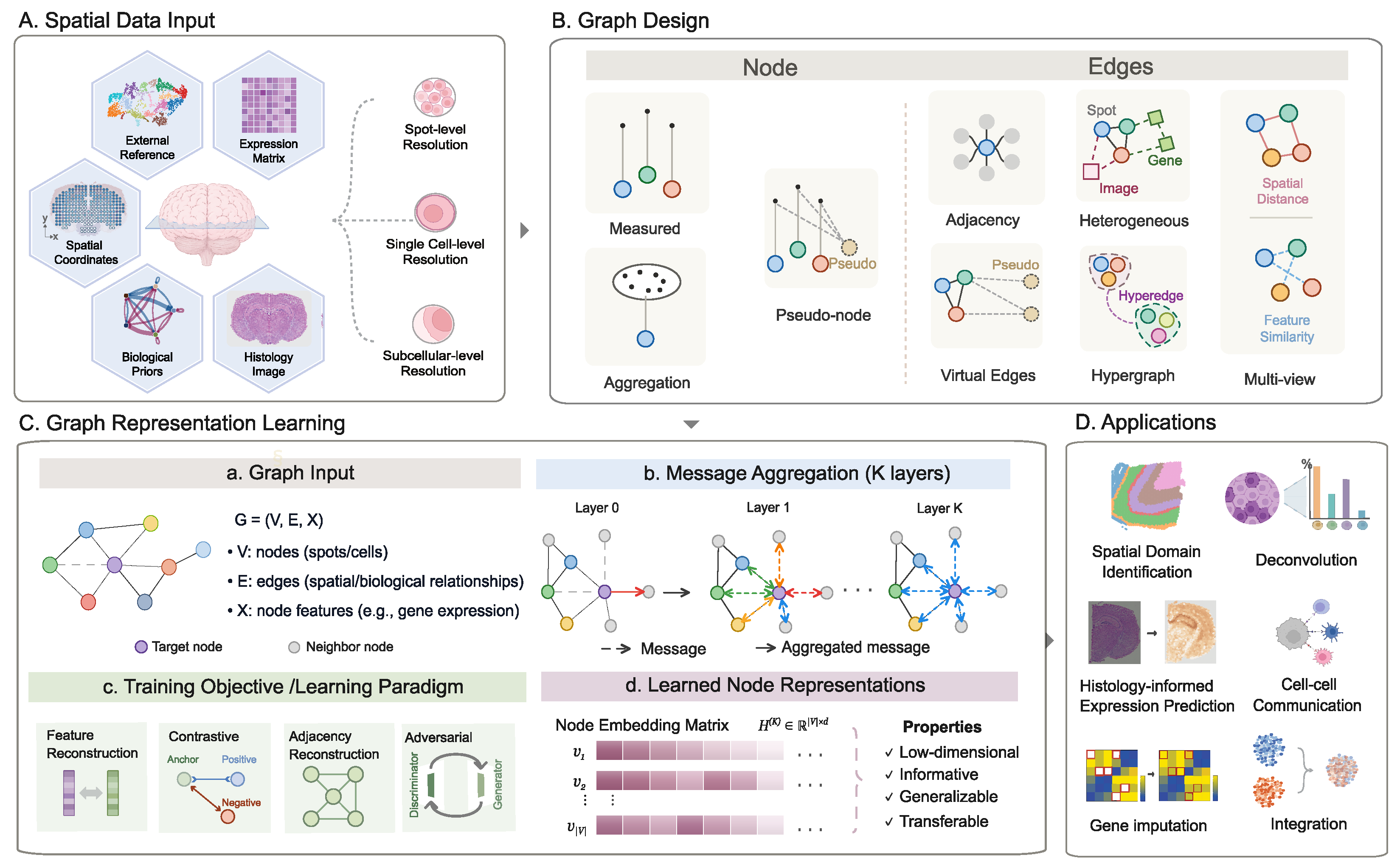
Figure 2.
Design matrix of representative ST-GNN methods organised by downstream task. The rows cover six task categories: spatial representation and domain identification; integration, alignment, and mapping; cell–cell communication and niche inference; imputation and denoising; deconvolution; and expression prediction from histology and super-resolution. The columns summarise node types, edge evidence, graph construction, graph roles during learning, GNN operations and learning systems, model outputs, and training objectives. Filled circles mark the main design categories selected for each method rather than every implementation detail. The matrix provides a visual summary of the representative methods discussed in the main text and is not intended as a complete catalogue of ST-GNN methods.
Figure 2.
Design matrix of representative ST-GNN methods organised by downstream task. The rows cover six task categories: spatial representation and domain identification; integration, alignment, and mapping; cell–cell communication and niche inference; imputation and denoising; deconvolution; and expression prediction from histology and super-resolution. The columns summarise node types, edge evidence, graph construction, graph roles during learning, GNN operations and learning systems, model outputs, and training objectives. Filled circles mark the main design categories selected for each method rather than every implementation detail. The matrix provides a visual summary of the representative methods discussed in the main text and is not intended as a complete catalogue of ST-GNN methods.
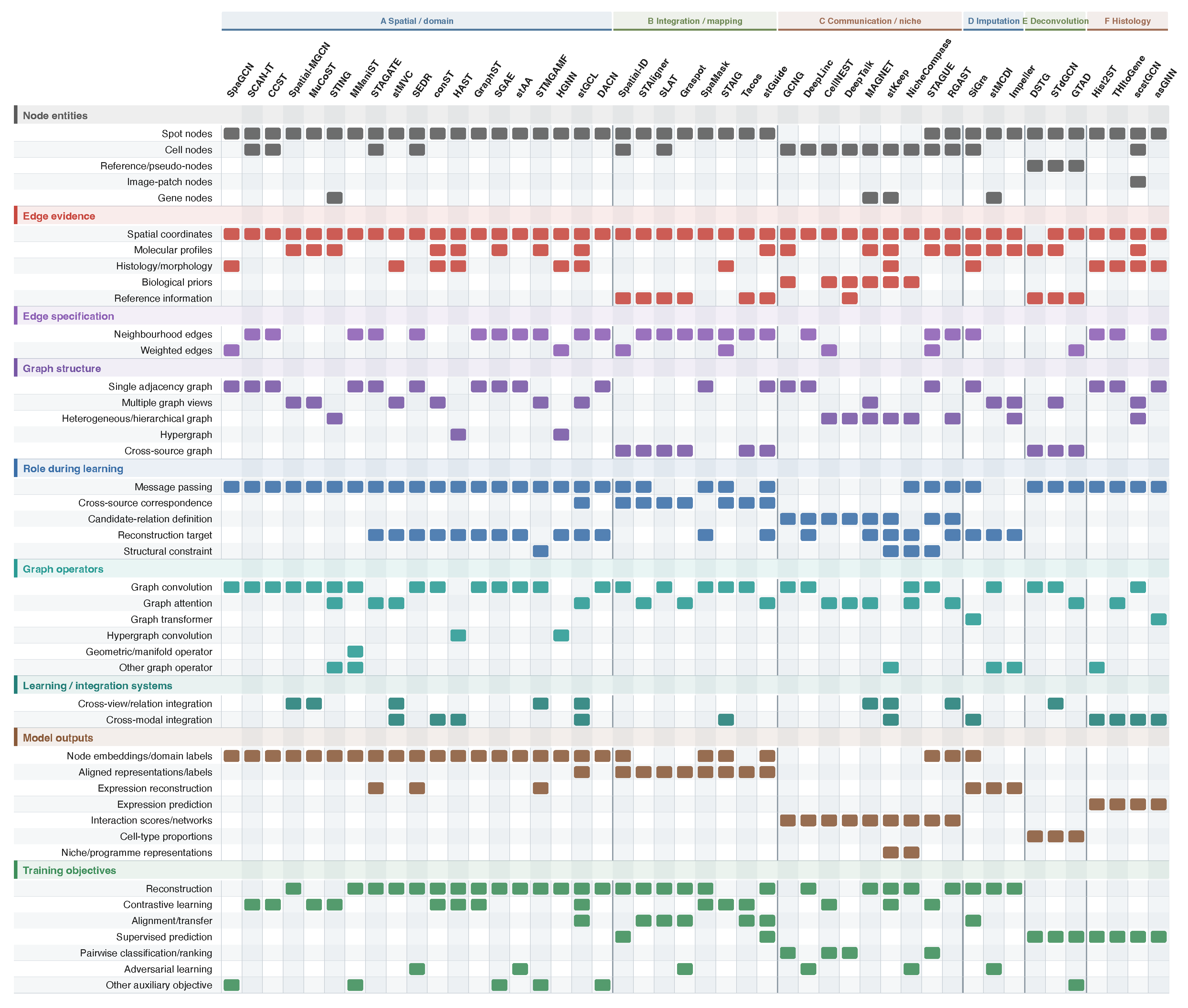
Table 2.
Analytical modes and validation evidence for ST-GNN outputs. The six downstream task categories are grouped by output type into representation and recovery, relational inference, and mapping and transfer across sources. For each mode, the table specifies the role of the graph, the model output, the conclusion supported by that output, and the evidence relevant to its evaluation.
Table 2.
Analytical modes and validation evidence for ST-GNN outputs. The six downstream task categories are grouped by output type into representation and recovery, relational inference, and mapping and transfer across sources. For each mode, the table specifies the role of the graph, the model output, the conclusion supported by that output, and the evidence relevant to its evaluation.
| Analytical mode | Role of the graph | Model output | Supported conclusion | Evidence needed for stronger interpretation |
| Representation and recovery | The graph provides spatial, molecular, histological, or multimodal context for representation learning and expression estimation | Embedding; domain label; denoised, imputed, predicted, or sub-spot expression | Spatially coherent groups, regional patterns, expression estimates informed by graph context, or predictions informed by morphology | Boundary evaluation; marker and histology support; held-out genes or locations; matched data at higher resolution; uncertainty estimates |
| Relational inference | The graph defines candidate interactions or represents connections among cells, genes, pathways, and local microenvironments | Interaction score; ligand–receptor score; inferred network; niche embedding; microenvironment programme | Candidate communication events, inferred interaction structure, niche organisation, or local microenvironment patterns | Validation independent of the construction prior; target-gene activation; spatial protein measurements; perturbation evidence; reproducibility across tissues or samples |
| Mapping and transfer across sources | The graph connects units across references, slices, samples, modalities, or query datasets while preserving structure within each source | Aligned embedding; correspondence; transferred label; cell type proportion estimate | Correspondence between data sources or composition estimates informed by a reference | Tests of structure preservation; marker retention; sensitivity to anchor selection; alternative references; comparability between reference and target data; independent validation |
Disclaimer/Publisher’s Note: The statements, opinions and data contained in all publications are solely those of the individual author(s) and contributor(s) and not of MDPI and/or the editor(s). MDPI and/or the editor(s) disclaim responsibility for any injury to people or property resulting from any ideas, methods, instructions or products referred to in the content. |
© 2026 by the authors. Licensee MDPI, Basel, Switzerland. This article is an open access article distributed under the terms and conditions of the Creative Commons Attribution (CC BY) license (http://creativecommons.org/licenses/by/4.0/).
Copyright: This open access article is published under a Creative Commons CC BY 4.0 license, which permit the free download, distribution, and reuse, provided that the author and preprint are cited in any reuse.