

Submitted:
27 August 2026
Posted:
31 August 2026
You are already at the latest version
Abstract
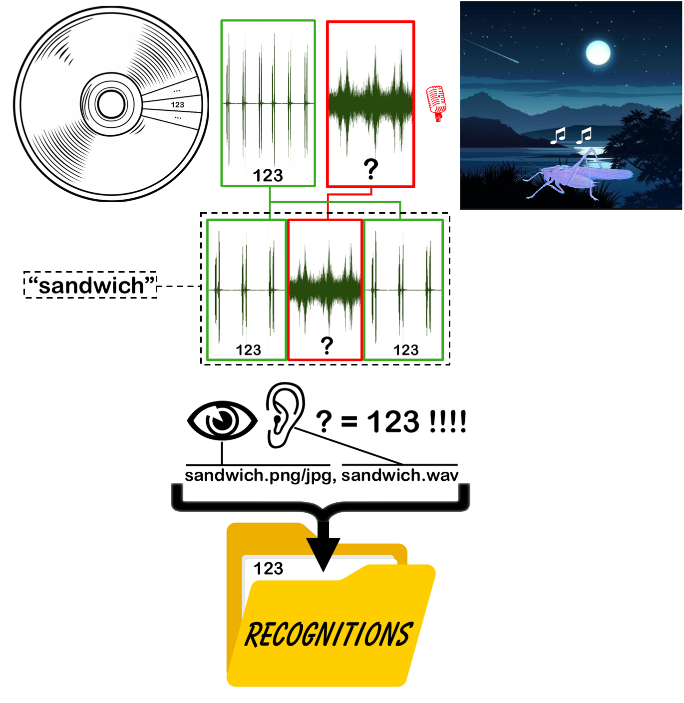
Field recordists often deal with situations where the presence of a species is documented exclusively by an audio file, without accompanying images nor physical specimens. Machine Learning (ML) classifiers trained on annotated datasets are increasingly popular for the automated identification of insect species from soundscapes or single-species recording. Such promising technology is generally reliable, but cannot correctly classify a species whose time/frequency patterns is not included in the reference datasets. Human experts cannot match the speed of a ML classifier but can provide the flexibility needed to overcome its limitations, by taking advantage of the digital audio software commonplace in the field of bioacoustics and of simple operations such as cut and paste. Such empirical comparisons are complicated by several factors, here individually addressed: guidelines are provided to mitigate the difficulties of specific recognition, both by emphasizing the nature of the obstacles, and by providing step-by-step procedures to overcome them. In light of a growing concern for the lack of verifiability in arthropod research, and a corresponding lack of repeatability in bioacoustic studies, and considering that science is the study of repeatable falsifiable phenomena with a methodology designed to minimize confirmation/cognition biases, the paper introduces the empirical “sandwich method”, that involves two audio files: “the filling”, a time slice of 2 seconds – or one echeme, if its duration exceeds two seconds – cut from the novel, unrecognized recording and inserted in “the bread”, the exemplary reference audio. On-screen view is then zoomed to “the sandwich”, a time window of six seconds (or at least three echemes) centered on the filling. Recognition is based on the similarity of bread and filling as observed side by side first visually (oscillogram), and then aurally (unaided ear comparison). Recognition of the poorly audible sandwiches can be improved by the frequency-lowering effect granted by playing the audio at lower speed (e.g., 1/4 or 1/10 of the natural speed) thanks to the special functions of the audio software. The method requires to save the decisive sandwich as an audio file and as a screenshot, thus ensuring persistence, verifiability, repeatability and possible redaction of the recognition.
Keywords:
orthoptera
; bioacoustics
; digital recordings
; expert recognition
; comparison workflow
1. Introduction
Field recordings of Orthoptera sound are frequently unaccompanied by the collection of physical specimens nor of still or moving pictures of the singing insect. Such situations are typical of the increasingly popular Passive Acoustic Monitoring (PAM) scenario, but also of active, supervised recordings, when no specimen was collected for practical impossibility or environmental concerns, and:
- the insect wasn’t seen or was barely seen (darkness, vegetation thickness, insect elusiveness, uncertain position of the sound source);
- the insect was seen but wasn’t recognized and no good photos were taken;
- images and specimens of more than one species are available, but none of them was seen singing during the recording (with uncertainty about which species was recorded).
When trying to identify a species by its song, based on previous experience a human expert may, or may not, recognize it. In the latter case, specific identification can be achieved by the comparison of, on one side, the novel digital recording and, on the other side, one or more digital audio files considered as a reliable reference for the identification of species (see section 2.2 “«Reference Recordings»: Generalities”). It should also be noted that the need to support the identification by comparison with existing audio may arise even when the song is recognized, e.g., whenever the recordist feels the need to corroborate the recognition by checking other reliable sources, or when the specific identification will appear in a scholarly publication, requiring a citation of the reference source used for the comparison.
Since a couple of decades, the popularity of Machine Learning (ML) classifiers, usually trained on annotated databases of digital sounds and aimed at the automated recognition of specific songs, is constantly increasing. While ML classifiers are usually very quick and effective, their reliability may vary greatly, as it entirely depends on the exhaustiveness of the training dataset, on the completeness and reliability of its annotations and on the degree of similitude between the time/frequency patterns stored in the dataset and those in the novel recording. While decisively effective for the recognition of common species, ML classifiers may incur in relevant problems such as the missed or erroneous recognition of song patterns that were not included – or were erroneously annotated – during the training phase. Intuitively, it’s quite obvious to understand that no system can recognize something that has never met before, and this may refer both to uncommon sound patterns by species included in the annotated dataset, or species entirely missing from it. Besides those limitations, the operation of such systems may pose stringent software, hardware and IT knowledge requirements out of the grasp of the individual researcher.
If provided with enough time and with commonplace digital audio software such as the following (Buzzetti et al., 2024), capable of playing audio files and to provide on-screen digital visualization of acoustic phenomena in the domains of time, frequency and amplitude:
- Adobe Audition 1.0,
- Syntrillium Cool Edit Pro,
- Audacity 3.6 (https://www.audacityteam.org/),
- Raven Pro (https://www.ravensoundsoftware.com/),
- Rthoptera Shiny App (Rivas et al., 2025 - https://github.com/naturewaves/Rthoptera),
- Rthoptera Desk (Rivas, 2026 - https://github.com/panchorivasf/Rthoptera-Desk),
any human expert can compare novel audio files with those described in the 2.2 “«Reference Recordings»: Generalities” section.
Compared with the quick, efficient but not universally reliable ML classifiers, the human expert, not constrained by the exemplary training dataset nor irreversibly driven by annotations, can perform comparisons between any pair of digital audio files of suitable quality, can base his/her decisions on more numerous, more diverse and more flexible criteria and, when needed, can improve the comparability of the two terms of comparison by preprocessing one or both files as needed to improve the reliability of the specific identification.
Since 2014, the authors have been trying to define and divulge guidelines for the successful comparison of heterogenous digital recordings. While using one’s own sight and hearing in the comparison process may look very trivial, many technical and physiological factors concur in complicating the scenario. Most of those factors will be addressed in the Introduction, while the Guidelines will describe as punctually as possible the mitigation strategies.
Only a bare minimum of bioacoustic terminology will be used in the acceptation by Baker & Chesmore (2020) and bibliography therein, that for our purposes can be simplified as follows:
- Tooth impact: indivisible fundamental unit of sound, that can be visually resolved at a millisecond scale in the carrier wave: depending on the tegminal vibration mode, one or several amplitude cycles (elementary oscillation in the carrier wave) can be promoted by a tooth impact (see Bailey & Broughton, 1970 and bibliography therein);
- Syllable: first order aggregation of tooth impacts. Previously and contentiously defined as the fruit of a full bidirectional cycle of the stridulatory apparatus;
- Echeme: first order aggregation of syllables;
- Echeme-sequence: first order aggregation of echemes.
The contentious terms of “tick” and “zip” were formally introduced among the “human ear terms” by Morris et al. (1989) to define “noisy” sounds lasting less than one second, respectively without and with infrastructure (“infrastructure” is itself is an ill-defined concept, among those criticized by Baker & Chesmore, 2020). The Q (for “Quality”) factor (Green, 1955; Elsner & Popov, 1978) will be mentioned:
- the spectral energy of high-Q songs, typical of Grylllidae and widespread among Ensifera, is concentrated in a few narrow bands, giving a tonal, harmonic character to the song;
- low-Q songs, typical of but not limited to Caelifera, that lack frequency-selective tegminal structures, are more akin white noise: spectral energy is more evenly distributed and the resulting sound can be described as swishing or rustling.
Concerning the visual representation of acoustic phenomena, the following terminology will be adopted:
- Time/Amplitude Envelope (TAE) – the time (x-axis) history of amplitude (y-axis), also commonly called waveform or oscillogram, describing the perceived volume in time;
- Spectrogram or Time/Frequency Spectrum Image (TFSI) – the time (x-axis) history of frequency (y-axis) distribution, with a color or B/W intensity scale representing the amplitude associated with the different frequencies;
- Mean Spectra (MS) – the amplitude (y-axis) at the different, increasing frequencies (x-axis). Amplitude is averaged with reference to an interval of time. This visualization of spectral energy also goes under the name of “frequency profile” or “frequency analysis”.
1.1. Required Level of Technical Proficiency
To deliver sensible, consistent and reliable results the human expert must have a good first-hand user experience in at least one of the software listed above. The minimum required operational skills include the following:
- Opening audio files.
- Saving copies of an audio file under different names.
- Working with multiple open files.
- Visualizing TPE and spectrograms.
- Zooming in and out to shorter or longer time intervals.
- Applying positive and negative amplification.
- Applying filters (it’s advisable to use the highest order available).
- Generating MS.
- Cutting and pasting sound snippets among different files.
- Playing the sounds at normal speed.
- (optional) Saving the file at a different sampling rate.
- Using the time stretch function to play sounds at reduced or increased speed: when used to bring inaudible ultrasounds down into the human hearing range, the stretch function generates a sound that is longer and lower-pitched than the original. It’s important to understand that the time-stretch mode we refer to is the one that preserves the natural relation between time and frequency, thus implying an alteration of the wavelengths as time is compressed (pitch gets higher) or extended (pitch gets lower). Respectively, those are the cases of a 33-rpm LP record played at 45 rpm, or vice versa. Depending on the wording adopted by the different software interfaces, it may be described as the option that does not preserve pitch nor tempo, or as the option that changes speed and pitch. When time-stretching a sound to more than 10 times its original length, the pitch may get very low, in which case if further slowing-down is needed it should be applied with the “stretch time but preserve pitch” mode, so that the resulting audio does not exceed the lower threshold of human hearing.
All the technicalities relative to field recording of Orthoptera sounds are addressed in a set of twelve lessons, dubbed “The Twelve Pillars” (World Biodiversity Association, 2024). Here, only some hints are provided but any nature recordist should get the appropriate training, or self-educate, gaining a good grasp of the physics of sound, of the technical features of the recording equipment, and of the requirements for a good recording.
1.2. «Reference Recordings»: Generalities
In biology, general consensus exists about the concept of “type”, stemming from the provisions of Articles 72-75 of the ICZN (International Commission on Zoological Nomenclature, 1999), and about the requirement to deposit type specimens in an institution that maintains a research collection, with proper facilities for preserving them and making them accessible for study. In line of principle, the need to deposit specimens is not strictly limited to new taxonomic entities: as explained by Turney et al. (2015), for arthropod research to be verifiable, specimens representing the taxa on which the research is based should be made available. Such “voucher specimens” are “...labeled, curated, data-based specimens that have been deposited in a collection or museum, available for verification of the work and to ensure researchers are calling the same taxa by the same names. Voucher specimens themselves are the subject of research...”. The title of the paper by Turney et al. (2015) is explicit: “Non-repeatable science: assessing the frequency of voucher specimen deposition reveals that most arthropod research cannot be verified.” In the similarly titled paper “A deafening silence: a lack of data and reproducibility in published bioacoustics research?”, Baker & Vincent (2019) extend such observations to the bioacoustic domain, revealing a worrying scenario: at that time of their paper, only a minority (21%) of published papers in bioacoustic was accompanied by the deposit of recordings in a repository, supplementary materials section or personal websites. As a way to mitigate the lack of reproducibility, Baker & Vincent (2019) advocate the collection and deposit of “voucher sound recordings” (preferably associated with a voucher specimen or at least subject to the same level of curation and accompanied by equally exhaustive data).
Even though we didn’t perform any statistical research, the situation does not appear to have radically improved since 2019, as it’s currently very frequent that new bioacoustic papers are unaccompanied by any accessible voucher sound recording. The crisis in the verifiability of bioacoustic research may also stem from the lack of universally recognized technical guidelines for “acoustic types” as defined, e.g., by Rivas et al. (2025), who candidate their Rthoptera software to support the descriptive phase of new acoustic type material.
While the repeatability of Orthoptera research is jeopardized by the absence, or the insufficient number, of voucher audio samples or any similar kind of acoustic type material recognized and divulged as such, fortunately in recent decades digital audio files have been accumulating in public repositories, both curated by experts and based on citizen science, or have been collected on digital media accompanying monographs about the Orthoptera. While the scientific reliability of some specific attributions of digital audio in citizen science projects may be questioned, curated or scientifically published sources are generally trustworthy and can be used to cross-check non-curated recordings.
To the purposes of this paper, the concept of “reference recording” encompasses digital audio files containing Orthoptera songs in the following categories:
- the publicly accessible voucher sound recordings deposited as supplementary material of scientific publications,
- the recordings uploaded in curated or non-curated Orthoptera-themed repositories (see section 2.6.2 “Sources of reference recordings”),
- the recordings on the digital media that accompany scientific monographs,
- novel recordings by any recordist that have been reliably attributed to a species following the guidelines and methods outlined in this paper.
Regardless of such categories, as the commonest and less elusive species are recorded more frequently, it’s obvious to expect shortage or absence of audio files relative to the uncommon species.
1.3. Unavailability of Species-Level Matching Reference Recordings
1.3.1. Objective Unavailability: Not an Orthopteran! Small Cicadas and Other Soniferous Insects
Any recordist engaged in the collection of Orthoptera sounds should have some knowledge of the song of some less common but widespread species of cicadas whose song may resemble that of an Orthoptera. One such species is Tettigettalna argentata (Olivier, 1790) whose song was misidentified by author CB as that of some Barbitistes (Charpentier, 1825) for a long time, but many others can be found on websites such as Cicadasong.eu (see the “References” section).
Other soniferous insects, including buzzing Hymenoptera, Heteroptera and ants, can sometime be recorded inadvertently, but usually the source of such sounds is easily identified. In any case, if in doubt, extend your attention to other insect orders.
1.3.2. Objective Unavailability: Incompleteness of the Acoustic Record
It’s perfectly possible that a novel recording has collected a previously unreported time/frequency pattern, in which case no exact match will be found among the reference recordings. If the new patterns bear some resemblance to reference recordings and other details (geographic location of the recording station, season...) suggest a shortlist of candidate species, it’s possible that the novel recording represents an uncommon pattern by one of the candidate species. Only radical differences allow to hypothesize the presence of an unreported species, in which case the possibility of an encounter with a new-to-science taxon is marginal, the most plausible explanation being the presence of a still unreported, or not adequately reported, allochthonous taxon, an increasingly probable event in times of climatic change.
A much more frequent possibility is an encounter with a well-known species outside of its reported area, that adds new localities to the known distribution, aka “filling with dots” practice. Both elusive and night-singing species are not easily detected and one cannot assume that an exhaustive, fine grained entomological explorations took place in the recording area. Considering the recency of bioacoustics as a scientific discipline and the low number of nature recordists, it’s perfectly plausible that a bioacoustic survey collects evidence of taxa previously unreported for each area. As a consequence, while preparing a list of candidates based on taxa reported for the area is very advisable, such lists should never be regarded as exhaustive, and also taxa reported in similar environments (consistent for elevation, vegetation and kind of landscape) should be considered as plausible candidates.
1.3.3. Objective Unavailability: Gender-Specific Orthoptera Songs
Based on our current knowledge and waiting for future studies, a song can, or cannot, be identified at a specific level. The latter is the case of, e.g., the genus Eupholidoptera Mařan, 1953. The species of Eupholidoptera living in the Italian territory deliver a song whose interspecific variability does not exceed the intraspecific variability. In such cases, the recordist should take into account the reported geographical range of the taxa involved. The same song may – depending from the location – be attributed to, e.g., E. chabrieri (Charpentier, 1825) if recorded in Piedmont, E. schmidti (Fieber, 1861) if recorded in Emilia Romagna, E. magnifica (A. Costa, 1863) if recorded in Sardinia. Other cases include all the species of Gryllotalpa Latreille, 1802 whose range overlaps that by G. gryllotalpa (Linnaeus, 1758), that deliver a similar song and can be distinguished only by the chromosomal count. In other words, these are two genera whose species produce the same sound but are genetically different (Allegrucci et al. 2013; Broza et al. 1998).
1.3.4. Subjective Unavailability: Incapacity to Recognize a Good Matching Reference Recording
This may be caused by inexperience, and can only be solved by external advice, or by repeated attempts using the same or, advisably, different reference recordings of the candidate species, taking into account the information provided in this paper about the influence of temperature on song delivery, about the technicalities involved in the comparison of audio files, and about the need to strive for excellence during the recording phase.
1.4 Technical (Dis)Similarities Between Digital Audio Files
1.4.1. The Unrealistic Conditions for Perfect Comparability
Regardless of their content, the degree of comparability of two digital recordings depends on the technical affinity of the devices and of the processes by which they were obtained. Low comparability may result in laborious, indecisive, complicated or plainly impossible comparisons. Technical evolution in time and the wide and constantly growing range of recording devices complicate the scenario, and the idea that different recordists in different times may engage the same subject with identical equipment and environmental conditions is – to say the least – highly improbable. Yet, just for the purpose of understanding the most relevant factors at play, the following list cites the main aspects by which two digital recordings of the same Orthoptera species may differ. It’s uneasy to rank such factors by importance: to say one, environmental conditions may affect decisively the outcome of two recordings made with the same equipment, and technical factors may make incomparable two recordings of the same subject performed simultaneously in identical environmental conditions:
- recording distance (from microphone to singing insect),
- air temperature,
- exposure to sunlight,
- microphone polar sensitivity pattern,
- microphone dynamic response,
- gain settings (microphone and recorder),
- sampling frequency,
- postproduction: any intentional intervention, such as filtering, that may alter the original recording.
Some of such factors will be shortly treated hereinunder.
1.4.2. Different Sampling Frequency: “Audible Range” vs. “Wide Band”
Technicalities beyond the scope of this paper influence the format in which digital recordings are stored, played and analyzed. The main distinction is related with the sampling frequency of the equipment (microphone, recorder and software) used in the recording phase, in other words by the number of elementary sampling actions (amplitude or “acoustic pressure” readings) performed in a unit of time. As shown by the Nyquist–Shannon sampling theorem, the amplitude of the recorded frequency band is bound at the top by exactly half the sampling frequency. Considering the theoretical upper limit of human hearing at around 20 kHz, sampling frequencies of 44.1 kHz and 48 kHz (also called “CD standard”) deliver “audible band” recordings while (if supported by adequate equipment) a sampling frequency of 96 kHz, by engaging a recorded band up to 48 kHz, encompasses the low inaudible range. In the last two decades, equipment operating at higher sampling frequencies, such as 192 kHz, 250 kHz or 384 kHz, has become available and increasingly cheaper. Capable of delivering “wide band” recordings, up to 192 kHz of maximum recorded frequency, such wide band equipment is the state-of-the-art technology. For what concerns the comparison of two digital audio files, it’s obvious that if they differ in the technological standard (current and obsolete, in other words wide band versus audible band) complications may arise, many of which will be addressed here.
1.4.3. Different Microphones: Dynamic Response and Polar Sensitivity Pattern
The technical features of the microphone are of paramount importance. All other things, including sampling frequencies, being equal, the use of different microphones may result in radically different recordings. The two most relevant technical factors are:
- dynamic response – it defines the microphone’s responsiveness to the different frequencies. While a perfectly flat dynamic response curve would be preferrable, it’s more frequent for microphones to excel in a portion of the dynamic range. Usually, “ultrasonic” microphones are optimized for the inaudible frequencies and perform poorly (“are too hard”) in the audible range, a limitation partly overcome by multi-capsule microphones where an “audible range” and an “inaudible range” capsule work in parallel, as in the case of Dodotronic Ultramic 384K EVO;
- polar sensitivity pattern – it defines the microphone’s selectiveness in directionality, ranging from omnidirectional to very directional. While the use of a parabola may increase the directionality of a microphone put in its prime focus, the use of parabolic microphones is strongly discouraged, because of the inherent filtering and selective amplification characteristics of every parabolic reflector.
As the microphone influences the amplitude of the sounds recorded throughout its native frequency range, the effects of the use of different brands and models concur with the contingent factors at the moment of recording in shaping the TAE and the spectrogram and, obviously, the timbre perceived by the human ear. Figure 1 is proposed as an example of the effect of different microphones and equipment on three recordings of the same species, Decticus albifrons (Fabricius, 1775), obtained in similar conditions and limited to the 5 kHz – 12 kHz band by low-pass filtering. The three mean spectra are laterally shifted depending on air temperature at the recording site. While the general profile of the MS remains recognizable, details differ due to the radical technical differences of the microphones, one of which is nearly omnidirectional. Despite such differences, tentatively homologous features (peaks and valleys) can be observed in the three MS, and are marked in Figure 1.
1.4.4. Different Gain Settings
The same equipment at the same distance of the same insect at the same temperature may deliver radically different results, depending on its gain settings. Gain is a physical quantity that can be imagined as a voltage multiplier that is applied before the analog to digital conversion takes place. Many microphones and recording devices include a user-controlled gain setting that may be continuous or, more frequently, in three or more discrete categories. “Medium gain” is the general, all-around setting, a compromise that preserves a good level of responsiveness to feeble components while avoiding a prevalence of background noise. The recordist should try all the available settings, but should not give in to the temptation of using the maximum gain setting that, unless exceptionally favorable ambient conditions are granted, results in overwhelming noise and in frequent clipping of the foreground sounds. On the other side, minimum gain, while granting a lower presence of noise in the recording, unless the microphone is in very close proximity to the singing insect will result in the loss of the feebler spectral components, and hence in a recording unsuitable for spectral or temporal analyses.
A more technical treatment of the concept of gain, including digital gain and microphone port gain, is outside the scope of this paper.
1.5. Relevant Conditions During the Recording Phase
1.5.1. Distance and Orientation of the Microphone
The relative position of microphone and sound source ranks among the very few top reasons why a recording may result suboptimal or unsatisfactory, or different from a reference recording taken in ideal conditions. In particular when taking wide band recording, considering how divergence and atmospheric absorption selectively attenuate the higher frequencies, maximum effort should be put in placing the microphone at the closest distance to the insect, regulating the gain consequently. The orientation of the microphone should engage the subject at the most pronounced lobe of its polar sensitivity pattern, guaranteeing the nominal response of the microphone capsule.
Such conditions can be taken as granted only in the very favorable scenario of studio recording with the insect in an anechoic enclosure, but novel and reference recordings obtained on the field cannot always grant a constant positioning of the microphone respective to the sound source, even more so when the source is not clearly seen (e.g., night recordings). A relatively common circumstance when recording an unseen Orthopteran is pointing the microphone not at the insect, but at a reflection of its song (a wall, a hedge, the ground itself...). It’s suggested to scan the space radially from the recording position to ascertain whether another direction provides a clearer signal.
1.5.2. Air Temperature
Reference recordings taken at a given temperature may look very different from novel recordings of the same species, taken at different temperatures. As it can be easily observed, air temperature influences both the duration and the rate of emission of Orthopteran songs, respectively, in an inversely proportional and directly proportional fashion.
The Arrhenius equation, describing the exponential dependence of the rate constant of a chemical reaction on the absolute temperature, is important in that respect: the temperature dependence arises because a greater fraction of molecular collisions have sufficient energy to exceed the activation barrier as temperature increases. Its classic form is as follows:
- k is the rate constant (frequency of collisions resulting in a reaction),
- T is the absolute temperature,
- A is the pre-exponential factor or Arrhenius factor or frequency factor. Arrhenius originally considered A to be a temperature-independent constant for each chemical reaction. However more recent treatments include some temperature dependence,
- Ea is the molar activation energy for the reaction,
- R is the universal gas constant.
Dolbear’s Law (Dolbear, 1897), an inference applicable from a temperature of around 60 °F/21 °C, where the reference species Oecanthus fultoni Walker, 1962 sings at a rate of 80 echemes/min, can be considered as a particular case of the Arrhenius equation:
- TF is the air temperature in degrees Fahrenheit
- N60 is the number of chirps per minute.
There are species, such as Cyrtaspis scutata (Charpentier, 1825), who sing also at very low temperatures, in which case the echeme duration (up to 125 ms) if compared with the song delivered in the hottest days of summer (under 15 ms) may stretch by a factor of 8 or more (See section 4.1 “Variability of Temporal Patterns”). Even when less dramatic, the temperature-related compression of the echeme duration may result in the obliteration of its typical structure: the typical waveforms may disappear as the intervals between syllables decrease. More under, the “Case Study” section includes temperature-related information about the song of Pseudochorthippus parallelus (Zetterstedt, 1821) and C. scutata.
1.5.3. Naturogenic, Anthropogenic and Technogenic Noise
Assuming that reference recordings are selected for quality and often are obtained under favorable conditions, for what concerns novel recordings noise is anyway an omnipresent adversary, very likely to affect the recordists’ activity in its three canonical forms:
- naturogenic: caused by nature, including wind, homospecific and heterospecific songs, water flowing, rain etc. Among the most annoying factor for recordists interested in Orthoptera sounds is the concurrent song produced by cicadas or by widespread and very loud species, such as Tettigonia viridissima (Linnaeus, 1758), that obliterates the concurrent song of species delivering a feebler song. As a side note, the sound of running water is unexpectedly strong in the inaudible range: recording in the vicinities of a fountain or of an open tap may be completely useless;
- anthropogenic: directly caused by humans, including the recordist himself or herself. Examples abound: walking, talking, breathing, coughing, sneezing, touching the recording equipment or the vegetation, etc.;
- technogenic: caused by technical devices, such as cars, production plants, railroads, electric lines, chargers and low-energy light bulbs etc. It’s particularly present and annoying also in the inaudible range.
Most digital audio software, including some of those listed above, include special functions for noise reduction. While sometimes effective, such functions are destructive and radically alter the sound, to the point where a de-noised audio file is unsuitable for analytical purposes, including comparisons with unaltered reference recordings. Skilled bioacousticians can obviously apply the noise reduction functions to copies of the original file during the identification process, provided that the altered recording is not uploaded nor used for analyses. Some simpler forms of noise reduction, such as hiss reduction, are a little less invasive and can bring some advantage, if appropriately adopted by competent users, who can self-train using the user guides of each software. Anyway, whenever the noise is concentrated in frequency bands not engaging the interesting song, or engaging it marginally, filtering is the most appropriate solution, as illustrated in the “Case Study” section.
While noise can be at least partly mitigated by filtering, the correct solution is prevention: striving to obtain the ideal recording conditions, and repeating the noisy recordings if the chance is given.
1.5.4. Number of Insects Singing
Comparing an audio file where multiple individuals are singing with one containing just one song may be arduous. Author CB incurred in a particular case where the concurrent song of different individuals of a species was intermeshing in time in such a way, that its TAE resembled closely that of another species.
Extreme cases apart, to complicate recognition it suffices that the echemes of two or more individuals overlap. Among the characteristics that may get lost when many individuals sing together, we cite the echeme emission rate and the echeme duration: only in case that just one individual is in the foreground, its echemes may be distinguished by their equal and higher amplitude but, if the echeme amplitude increases or decreases gradually, its exact initial and final instants may be invisible in the TPE, being covered by the concurrent background sounds.
1.6. Quality Issues and Recommended Standards
1.6.1. Reference Recordings
It can reasonably be assumed that the average quality of novel recordings is below the average quality of reference recordings: in a general sense, expert-validated reference recordings available in institutional repositories, as well as those in commercially issued CD’s or DVD’s, were subject to some editorial selection process, and – regardless of technical obsolescence, addressed more under – can be expected to show good to excellent quality, in particular if obtained in controlled conditions such as anechoic chambers in a laboratory setting. Furthermore, exemplary recordings can be post-produced (e.g., by filtering) to improve their clarity.
While throughout this paper the usage of the state-of-the-art equipment such as high sampling frequency (e.g., 384 kHz) recorders and microphones is strongly advocated, the acoustic record of Orthoptera – with particular reference to correctly attributed recordings in institutional repositories – is mostly in the audible range, at a sampling frequency of 44.1 kHz and, less frequently, of 48 kHz and 96 kHz. The digitization of analog (e.g., magnetic tape) recordings took mostly place in the last decades and – with a few exceptions – was typically aimed at obtaining digital files covering just the audible range. While the usage of obsolete equipment is now inexcusable, one cannot expect that reference recordings reflect the current recording technology. This very frequent technical mismatch is described in more detail and addressed more under.
Regardless of the possible format obsolescence, in specific cases reference recordings may be suboptimal and leave much to be desired in recorded amplitude (“volume”), duration or noise level. There is no remedial action for the objective unavailability of adequate reference recordings, but the technical hints provided more under may help in taking the best possible advantage of any recording, including some of the poorest.
1.6.2. Sources of Reference Recordings
Besides the off-line resources such as monographs that include a CD, e.g., Massa et al. (2012), several publicly accessible online sources of Orthoptera sounds are available: repositories such as Xeno-Canto (2026) comply with the requirement of data consistency and completeness, by providing preset alternative options or drop-down lists of preset values for several mandatory data fields, including a curated species list, and an interactive map. Other generalist repositories, such as iNaturalist, while taking advantage of preset species lists, require that just by a bare minimum of temporal and geographical data is supplied when uploading the audio file.
- iNaturalist - https://www.inaturalist.org/observations?sounds&taxon_id=47651 (more than 58,000 recordings)
- Xeno-Canto - https://xeno-canto.org/ (more than 37,000 Orthoptera recordings)
- Orthoptera Species File - https://Orthoptera.speciesfile.org/ (more than 2,000 recordings)
- Singing Insects of North America (SINA) - https://orthsoc.org/sina/
- Songs of Insects - https://songsofinsects.com/
The reliability of specific identification may vary and is higher in the case of supporting material of scientific papers (voucher sound recordings) and of curated sources like Orthoptera Species File, Xeno-Canto and SINA, but may not always be complete, such in the case of iNaturalist. If in doubt, prefer curated sources or download relevant scientific publications that include an unequivocal description of the specific song under study. See also section 3.2 “Selecting Appropriate Reference Recordings”.
1.6.3. Novel Audio
Complex factors including insect elusiveness as well as naturogenic, anthropogenic and technogenic noise will very likely affect any novel recording. While also the nature recordist can post-produce the audio files and can discard the unsatisfactory ones, good or excellent quality is the fruit of time and of an active commitment to excellence. For those reasons, if the same unidentified species appears in more novel recordings, only the best one, or the very few better ones, should be used for comparisons with reference recordings.
Due to the almost complete lack of control by the recordist on recording conditions, Passive Acoustic Monitoring (PAM) is the context in which novel recordings necessarily show a suboptimal or unsatisfactory quality. Brizio et al. (2024), introducing the concept of a species-specific “Surviving Acoustic Signature” (SAS), is entirely dedicated to the description of a methodologic pipeline for processing and recognizing individual specific songs from PAM recordings. See section 3.11 “Example of a Repetitive Pipeline for PAM recordings”.
In a general sense, considering that they can be obtained with state-of-the-art equipment, the technical inadequacy of novel recordings is inexcusable. The influence of unavoidable adverse factors linked to species elusiveness and field atmospheric and noise conditions, can be remediated only by improving the proficiency of the recordist or by further novel recordings obtained in more favorable conditions. The problem of recording quality is extensively addressed by Brizio et al. (2024). A few of the most relevant properties of a good recording include:
- One-channel (monophonic) recording (stereo recording can be resampled to mono recordings by all the audio software cited above);
- Minimal duration of at least a few discrete echemes (that may require more or less time, depending on echeme duration and echeme emission rate) or, for uninterrupted echemes as continuous trills, at least ten seconds;
- Recording obtained in very close proximity with the subject;
- Possibly, the song should be delivered by a single individual. If conspecific songs are present, it’s important that non-overlapping echemes are present in the recording;
- Absent or minimal background sounds and noise;
In the digital recording community, there is general consensus about the fact that record settings should engage the full dynamic range of the equipment, thus optimizing signal-to-noise ratio, and at the same time they should leave some headroom for post production intervention that may include amplification. As reported in many sources including a post of sound engineer “Mojo” on Medium (see references) the vox populi standard is setting the equipment so that:
- the peaks are kept away from the destructive clipping threshold of 0 dBFS, and do not exceed -6 dBFS / -5 dBFS;
- the average volume of the interesting sound is at least at -15 dBFS.
The two conditions are uneasy to meet for songs with very strong peaks and a feebler body.
2. Guidelines
2.1. Selecting Appropriate Novel Recordings
See section 2.6.3 “Quality Issues and Recommended Standards – Novel Audio”. Minimal requirements for novel recordings include the following:
- Only the best recording, or the very few better recordings, available for the same unknown species should be used in the comparison process;
- Recording should be unclipped, at least in the sections containing the unidentified song;
- Peak amplitude in the investigated section should be as near as possible to -6 dBFS;
- It’s perfectly admissible to preprocess one’s own new recordings to improve their recognizability by filtering, amplifying etc. but, as clarified more under, it may be wise to apply the same filtering also to the reference recording.
2.2. Selecting Appropriate Reference Recordings
Factors to consider include:
- Overall quality: Online repositories such as Xeno-Canto support a rating system (with score assigned at the recordist’s discretion), allowing the selection of the better reference recordings.
- Technical similarity with the novel recording, in particular for what concerns the sampling rate.
- Recency, a good clue of technical adequacy. A record from 20 years ago was most probably obtained with equipment very far from the current technical standards.
- Ideal recorded amplitude (“volume”), as for the novel audio.
- Reputation of the recordist or of the institution that provided the identification: even though a clear rating of the recordist experience is missing, there are indirect ways to assess reputation, including the public profile of the contributor available in the online repository, and platforms for scholarly publications such as SciProfiles, Academia.edu, Researchgate.
- Geographical area: if alternatives are available, all other things being equal, it’s better to select a reference recording from the same general area where the novel recording was taken.
- Period of the year: considering the influence of air temperature on the emission rate of the echemes, one should reasonably expect that, all other things being equal, two recordings of the same species from the same season will be more similar than when they refer to different seasons.
Obviously, once assigned to a species with reference to a reliable source and with a satisfactory degree of certitude, the recordist’s own audio files can be used as reference recordings, with the advantage that – if based on the same equipment – they will be technically consistent with the novel recordings being compared.
2.3. Pre-Selecting Candidate Species Based on Phenology and Ecology
Before beginning the shortlisting phase on bioacoustic bases, a relevant coarse-grained pre-selection may be based on the information available in the scientific literature, in particular by consulting monographs about the Orthoptera while asking ourselves “Which species may be singing here?”. Factors to consider include:
- known geographic distribution range: not forgetting what explained in section 2.3.2 “Objective Unavailability: Incompleteness of the Acoustic Record” about possible novelties, including an increasing presence of allochthonous and invasive species, one shouldn’t forget the famous quote by Dr. Theodore Woodward at the University of Maryland School of Medicine: “When you hear hoofbeats, think of horses, not zebras.” Generally speaking, species already reported for the area are better candidates than species never observed in the same region;
- known phenology of the species;
- known ecology, with particular reference to possible ecological constraints, such as elevation and ecoregion / plant community, habitat preference.
Only the species with compatible phenology and ecology should be considered as potential candidates. Among them, those already reported for the geographical area should be investigated first to speed-up the recognition process.
2.4. Using Image Collections to Shortlist the Candidate Species
Visual aids can be used to support a preliminary screening of candidates. To this purpose, the novel recording is loaded in the audio software, and visualized on the computer screen, typically as a TAE (waveform). Then, corresponding visualizations – printed on paper or collected in a digital file – are compared with the on-screen image to prepare a shortlist of candidates. Depending on the nature of the collection, digital or physical, the comparison may involve screen and book or, side by side on a split screen, audio software and a digital file, e.g., a pdf or a web page in a browser.
The most promising species will enter a shortlist and will one by one be considered in the comparison process described more under. Purely visual similarity between the on-screen audio and a raster image (digital or on paper) does not suffice to draw any conclusions. Only in the deplorable case when reference images are unaccompanied by any audio file, an uncertain decision may be taken based only on visual hints. Obviously, its reliability will be questionable until a digital audio file will be available and subject to a proper comparison.
Scientific publications may include images of TAEs, spectrograms and MSs. In particular cases, high-resolution images are made available digitally as Web pages, as in the case of Brizio et al. (2020) and Brizio et al. (2026). When comprehensive publications, such as Massa et al. (2012), are provided with a DVD or CD with sounds, the book frequently includes pages where the sonogram images (usually, in a small size) are orderly listed. Such pages can be described as a physical collection of images. If the publication itself is a digital file, then the pages with sonograms are themselves a digital collection.
Interestingly, if one commits to exclusively personal use, digital collections based on reference recordings can be made from scratch by any recordist. It suffices to load the reference recording in the audio software, then take a screenshot of the desired visualization, name aptly the captured image, and repeat for all the reference recordings. The image in the collection can then be assembled in a digital file whose format can be textual (e.g., a Microsoft Word file subsequently saved in PDF format) or hypertextual (e.g., a HTML file with clickable image tables). If the opportunity to self-produce a screenshot collection is taken, it’s advisable to include TAE’s at different time scales (10 s, 1 s, 500 ms, 1 echeme...) depending on echeme structure and duration. Figure 2 shows such a collection made for personal use by Author CB.
The audio files in repositories such as Xeno-Canto include sonogram and spectrogram previews that, due to their small size, cannot always be reliably used for shortlisting purposes.
2.5. Digital Audio Preprocessing
While time stretching and contraction will be applied during the comparison phase, the following preprocessing steps – all available as functions under specific menu entries of the audio software – can drastically simplify the comparison process. Some of the preprocessing steps may alter the audio file to the point of impeding its use for analytical purposes: before preprocessing, it’s mandatory to preserve a copy of the original novel recording under a separate name or, to the same purpose, to create a work copy under a separate name, and use that copy for the recognition attempts.
2.5.1. Trimming
As it will be illustrated in section 3.6 “Step by step Comparison Process – the Sandwich Method”, only a short excerpt of the novel recording will be used in the recognition phase. If desired, the recording can be trimmed, leaving only a few of the clearest echemes for the subsequent phases.
2.5.2. Removal of Silent Intervals
The visual and aural recognition process is drastically improved when repeated instances of closely packed sounds can be examined. While for the species that emit echemes at a regular and sustained rate the intervals themselves are a diagnostic character, for those that emit sparse or isolated echemes, the long intervals may be incompatible with the process described below. In those cases, since neither will be used to measure time-related quantities, it’s perfectly admissible to cut off the silent intervals, reducing them to a few tenths of a second, both in the novel recording and – if similarly affected by silent pauses – to the reference recording.
2.5.3. (Optional) Resampling Digital Audio: Downsampling
Downsampling is a destructive process and should be performed on a copy of the original recording. Only in case that the reference recording was obtained at a lower sampling rate, downsampling the novel recording to the same rate may improve the visual and aural similitude between the two. Most audio software includes automatic resampling features, described in section 3.6.2 “Automatic Resampling during the composition of the sandwich”. As illustrated in section 3.12 “The Filtering and Extreme Amplification Protocol”, alternatives to downsampling exist, and may be more effective in increasing the resemblance of two audio files obtained at radically different sampling rates.
No attempt at upsampling should ever be performed on either audio file: while downsampling compresses acoustic information actually present in the file, upsampling creates non-existing values by interpolation algorithms. The resulting audio is inherently unreliable and does not bring any advantage to the recognition phase.
2.5.4. Consistent Volume
As soon as the selected reference recordings are opened, it will become clear whether or not their recorded amplitude matches that by the novel recording. By applying digital amplification so that the amplitude of the echemes in the TAE is similar, the aural comparison described below will be easier and more convincing.
2.5.5. Consistent Filtering
As illustrated in the case studies, filtering may be necessary to isolate high-frequency echemes from noise or heterospecific songs engaging the lower frequencies. When the sampling rate of the two terms of comparison is the same, in case that the novel audio was high-pass filtered, it may look dissimilar from the reference recording unless the same filter is applied also to the latter, to increase the degree of similarity perceived visually or aurally.
2.6. Step-by-Step Comparison Process—The Sandwich Method
The process described here applies to audio files preprocessed according to the steps outlined above. The reader is reminded that – unless no audio file is available, a lack that will cast doubt on any conclusion drawn – no decision shall be based only on the comparison of printed or raster images of the TAEs or spectrograms. The subsequent acoustic comparison is mandatory, based on two audio files separately loaded in the audio software.
The process is illustrated in Figure 3. The description provided hereinunder is highly detailed but, in practice, not all the steps may be strictly required: recognition may happen at any step of the process, sometimes very quickly, even without adjusting the volume or the echeme emission rate of the exemplary recording.
2.6.1. The Sandwich Method
According to our experience, the quickest and most reliable recognitions are obtained by an empirical method that we informally named the “sandwich method”: “the filling”, a time slice of 2 seconds – or one echeme, if its duration exceeds two seconds – is cut from the the novel, unrecognized recording and is inserted in “the bread”, the exemplary reference audio. The proposed duration of 2 seconds is indicative: provided that equal time intervals are considered for the filling and for each slice, other comparable durations may work equally well, even though too thick slices (above 6 – 10 seconds) may slow down or hamper the process. On-screen view is then zoomed to a time window of six seconds (or three echemes). i.e., “the sandwich”, centered on the filling and encompassing two slices of bread of subequal duration, comparable with that of the filling. Recognition is based on the similarity of bread and filling as observed visually (oscillogram) and aurally (unaided ear comparison). As detailed more under, the recognition of the poorly audible sandwiches can be improved by the frequency-lowering effect granted by playing the audio at lower speed (e.g., 1/4 or 1/10 of the natural speed) thanks to the special functions of the audio software. The paragraphs that follow describe the method in more detail.
2.6.2. Automatic Resampling During the Composition of the Sandwich
During the composition of a sandwich, as described above, the filling is inserted into the bread. As clarified in Section 2.6.1 “Reference Recordings”, often the sampling frequency of bread and filling may differ. Fortunately, on opening a recording, among other data any audio software reads its sampling frequency. The same datum is available for any audio snippet created by copying or cutting a section of an audio file already opened. Based on such information, the software can automatically adjust the sampling rate when two different recordings are joined. Usually, as in the case of Adobe Audition and of Audacity (Figure 4A and Figure 4B, respectively), at the moment of pasting the filling is automatically resampled according to the sampling rate of the bread. Other software allows to compose the sandwich by merging (joining in their entirety) separate audio files, one for each component. In the case of Rthoptera Desk, resampling is controlled by user-defined parameters. The best results are obtained by aligning the sampling rate of the filling to that of the bread, as illustrated in Figure 4C. Resampling may adversely affect the volume of the filling, in which case it can be selectively amplified as illustrated in section 3.5.4 “Consistent Volume”.
2.6.3. Consistent Time Stretch of Filling and Bread
While not strictly required, this step allows to increase similarity between filling and bread. In particular, by time-stretching the filling, the effect of different recording temperatures is mitigated, and – subjectively – bread and filling will be perceived as more consistent in timbre. To decide the amount of time-stretch that should be applied to the filling, in case of discrete echemes their duration shall be measured both in the bread and in the filling. For trills and, in general, for very quick echemes, a zoom-in to a few hundredth of seconds may be required to observe syllable emission rate (trills) or actual echeme duration (ticks and zips). Once the different durations of corresponding song elements (1 echeme, 10 trills...) are written down, the stretch/compression factor is calculated. As an example, an echeme in the filling lasts 1.5 seconds, while an echeme in the bread lasts 2 seconds. Since 2 / 1,5 = 1.3333... , by stretching the original duration of the filling to 133% its original value, we will obtain a consistent echeme duration at the scale of the whole sandwich. If, vice versa, the echeme duration in the filling is slower than in the bread, by compressing to 75% (equal to 1,5 / 2) the duration of the filling we will obtain the consistency needed to spot similarities with more certainty.
The filling (and only the filling) is selected in its entirety and the requested time variation is committed to the audio file (by the OK or Apply button). As a very important warning, we remind the reader of the clarification about the time stretch function provided above in section 2.1 “Required Level of Technical Proficiency”.
2.6.4. Performing the Comparison: Sight and Unaided Ear
The recognition by visual comparison shall necessarily be corroborated acoustically: no decision shall be taken based on TAEs and MSs only. The aural comparison is mandatory to confirm the findings of the visual comparison.
-
Visual comparison
- ○
- The comparison is performed in TAE (waveform) view;
- ○
- To improve certitude or, vice versa, to discard vaguely similar candidates, it’s advisable to zoom-in to a time interval comprising the boundary between bread and filling, with one or very few echemes of each on the screen. By further zoom-ins and zoom-outs, differences at syllable level or at carrier level should emerge.
- ○
- In case of doubt, by passing to the spectrogram view the similarities or dissimilarities in the frequency patterns will help in drawing a decision. We remind the reader that the time resolution of the spectrogram is inherently poorer (more coarse-grained) than that of the TAE, so that a different sandwich (e.g., of 10 seconds for each bread slice and 10 seconds of filling) may be needed to appreciate the spectral similitudes or differences within the sandwich.
-
Aural comparison
- ○
- We strongly suggest the use of good quality earphones: loudspeakers can be used but the surrounding environment should be as silent as possible.
- ○
- For clearly audible sandwiches: the aural recognition attempt is performed by playing the sandwich at normal, natural speed.
- ○
- For barely audible or inaudible sandwiches: the aural recognition is attempted at reduced speed, typically at one quarter of the natural speed (one second = four seconds), but up to one tenth (one second = ten seconds) if needed. To preserve a realistic visualization of the sandwich after setting the desired decrease in speed, rather than actually applying the time stretch to the data, it’s advisable to use the “preview” feature to listen to the slowed-down audio without committing the changes to the audio file. By preserving the original file, successive attempts at different speeds can be previewed starting from the same audio.
- If obvious differences between the bread and the filling are perceived visually or aurally, the current filling is discarded (usually, a sequence of “undo” or Ctrl-z keys is sufficient to return to the original state of the novel recording before the insertion of the filling), then a different reference recording is selected and preprocessed, and a new sandwich is prepared.
- If relevant but indecisive similarities are observed, other reference recordings of the same candidate species can be tried.
2.7. Step-by-Step Comparison Process – Mean Spectra
Software such as Adobe Audition and Cool Edit Pro allows to perform successive spectral analyses on separate audio files, with the superposition of up to four mean spectra contours in the same window on screen, allowing a direct comparison of up to five MS. In other software, the MSs need to be separately generated and separately saved in as many images that, subsequently, can be paired on screen for a side-by-side comparison.
2.7.1. Check Again Volume Consistency
Even though the similarity in recorded amplitude was ascertained in the preprocessing phase, MS are generated by applying the Fast Fourier Transform algorithm to the temporal amplitude data in such a way that the frequency profiles of two digital recordings with similar volume may be vertically distant in the MS. While some degree of separation is desirable for ease of comparison, it should not get to the point where the on-screen window that contains the MS of the first does not entirely include the MS of the second. Zooming in and out and resizing the axes may help but, in some cases, a further amplification step may be needed to improve the vertical alignment of the two diagrams.
2.7.2. Selection and Scan of Consistent Time Intervals
To avoid the visualization of undiagnostic, momentary data at the cursor position, the relevant time interval should be selected by click and drag (or, depending on the software, by manual input of its limits), then the MS is generated by clicking the “scan” button (Adobe Audition) or the corresponding command. The process is repeated for the filling and for one of the bread slices.
2.7.3. Selection of the Most Relevant Frequency Window
Once the MS is available on screen, it’s sensible to restrict (zoom-in) the horizontal axis to the frequency where spectral energy is clearly evident above the noise floor. As shown in Figure 1, the MSs may be slightly displaced laterally, depending on the different temperatures at the moment of recording and from the dynamic response of the microphone. The frequency window should encompass the entire range of all the MS being compared, but should exclude both the empty section under the high-pass filtered (if applied) and the section above the highest frequency clearly attributable to the song.
2.8. Decisive Result: A Subjective Definition
Considering that the decision is based on a series of subjective visual and aural impressions, the degree of certitude attained may, or may not, be decisive. If based on recordings of suitable quality, the process should leave no doubt but, from the experience of the authors, it’s possible that the result is deemed uncertain, in which case one should wait until the quality of his own recordings improves as needed or until new reference records emerge from scholarly publications or are uploaded in public repositories.
2.9. Repeatability and Falsifiability
The method requires to save the decisive sandwich as an audio file and as a screenshot, thus ensuring persistence and possible redaction of the recognition. The file saving steps serve three equally important purposes:
- ensuring the scientific dignity of the process, by allowing anybody else to repeat the same experience and to challenge our conclusions;
- preserving the expenditure of time and energy invested in the recognition process: it’s perfectly possible that one forgets how a decision was taken and, after some time, new encounters with the same song may elicit the same doubts in the recordist, that may necessitate a reminder of how the past conclusions were drawn in similar cases;
- the solution of doubtful cases, especially those about barely audible or plainly inaudible songs, may be of interest for other bioacousticians, or may be required for a scientific publication.
Consequently, regardless of degree of certitude (failed recognitions may be as important as successful recognitions), at least one audio file enclosing the time breadth of the sandwich should be saved. Its name should be fully explicit, e.g., include as a bare minimum the following elements, separated by spaces, dashes or underscores:
- (optionally) a fixed suffix that marks its nature and purpose, such as “COMP”;
- a shortened but unmistakable version of the species in the reference recording, such as “P_PARALL” for P. parallelus;
- (optionally) a “vs” for “versus”;
- an acronym or reference number unequivocally identifying the source of the reference recording, such as “FI” for Massa et al. (2012), or “XC906734” for a Xeno-Canto recording;
- if needed (as in case of more localities covered by recordings taken in the same date), a shortened but unmistakable version of the name of the recording location.
- an unambiguous date/time reference of the novel recording being scrutinized, in a consistent format such as “2026-07-10-1800”;
Modern operating systems allow for long filenames. The bare minimum name structure illustrated above is just a suggestion, fully explicit names are encouraged. A filename example from Author CB is “Yersinella beybienkoi Fauna d’Italia vs Raticosa_20151024 142110.wav”.
Also, relevant screenshots (TAE and spectrogram of the sandwich, at different time resolutions if needed) should be saved as aptly named image files for future reference.
Usually, the discriminative skills of the recordist improve with experience and the unidentified or uncertainly identified recordings should be cyclically re-evaluated every few months.
2.10. Asking for Advice
Requests for external expert advice must always be accompanied by an audio file containing the novel recording, or by a link to an online repository where it’s stored, and by a detailed description of the failed identification attempts. Obviously, the availability of any expert to engage in time-consuming activity unrelated with their own research cannot be taken for granted. Digital sound repositories such as Xeno-Canto allow to mark any recording as “mystery” and often include a forum where unidentified recordings can be posted, accompanied by all the relevant information.
2.11. Example of a Repetitive Pipeline for PAM Recordings
If the novel recording is obtained with a PAM device, the reader is referred to Brizio et al. (2024) for all the specific problems and solutions. Usually, with several species recorded at the same time, heavy filtering is needed to separate frequency patterns attributable to each different species. Such patterns are degraded to the status of Surviving Acoustic Signatures (SAS), and should be treated as described in the workflow of Figure 5.
2.12. The Filtering and Extreme Amplification Protocol
Originally introduced by Brizio & Buzzetti (2014), a special comparison protocol may help overcome comparability issues between wide-band and audible-band recordings. Regardless of their superficial similarity, and to the fact that they will result in the coverage of the same frequency range, the two processes:
- Resample (downsample) to 44.1 kHz a wide-band recording (e.g., a 250 kHz or 384 kHz recording),
- Low-pass filter at 22.05 kHz a wide-band recording (e.g., as above),
are radically different and engage completely separate algorithms. The result of a downsampling operation will not necessarily be comparable (visually or aurally) with an audible-band recording, while – under favorable conditions – the result of the filtering operation may greatly enhance their degree of resemblance.
The dynamic response of “ultrasonic” microphones in the audible range is generally poor, especially when – as advisable to prevent excessive ambient noise – their gain is set to medium or low. It was particularly unsatisfactory in the otherwise excellent Dodotronic Ultramic 250 that the authors began using around 2010. Even when the insect song was clearly audible during the recording phase, the resulting digital audio – while preserving impeccably the inaudible frequencies – could barely be heard. The flowchart illustrated in Figure 6 was originally conceived to overcome such a limitation.
The U (Ultrasonic) recording obtained with the wide-band equipment is low-pass filtered at 21 kHz or at 22.05 kHz applying – when the software allows – the highest order of filtering (coincident with the steepest slope of the filtering function). The resulting audio file (LPFU for Low-Pass Filtered Ultrasonic) is then amplified until clearly audible components emerge, a fact that usually coincides with a higher clarity of the TPE. This may imply extreme amplification, up to +30 dBFS or more. If the current LPFU is sufficiently clear, it can enter the ordinary step-by-step comparison process described above.
Otherwise, it’s obvious that the wide-band microphone did not grasp sufficient audible components. If the opportunity arises, the recordist should not hesitate to repeat the recording, striving to get as close to the singing insect as possible, even when this means crossing the -0 dBFS threshold (“clipped recording”). Such an SCU (Subsidiary Clipped Ultrasonic) recording will be unusable for analytical purposes but, after low-pass filtering and aggressive amplification as described above, may provide enough audible components to allow a successful comparison.
The filtering + extreme amplification method is applicable only when the sampling rate in the two recordings is radically different: it should be considered an extrema ratio and should be applied only when the step-by-step comparison process described more under fails to deliver the expected results.
3. Case Studies
3.1. Variability of Specific Temporal Patterns
3.1.1. Pseudochorthippus parallelus (Zetterstedt, 1821)
Based on a YouTube video publicly released by Forstmeier (2023), it was possible to create Figure 7, that shows how a range of temperature variations of around 15° Celsius influences echeme duration and emission rate in P. parallelus. As verified with W. Forstmeier (pers. comm., 20 July 2026), the temperatures appearing in the video refer to the air temperature (in shadow) at the position of the recordist, while the actual temperature of the singing insect may vary and is tentatively indicated in Figure 7, based on the apparent position of the insect, that may be covered by layers of vegetation or sing in full light after an exposition to the sun of undetermined duration. Taking for granted the temperature of 18 °C in the shadow for the P. parallelus emitting the slowest echeme (2.83 s) and hypothesizing a temperature of 30 °C for the one emitting the shortest echeme (0.39 s), assuming a linear progression similar to Dolbear’s Law we may say that for every degree Celsius above 18 °C, echeme duration is reduced by around 0.2 s. Despite the inaccuracy of this simplification, that does not take into account the number of syllables emitted, most of which become indistinct in the quickest echeme, Figure 7 makes clear the inversely proportional relation between, on one side, air temperature and, on the other side, echeme duration and rate.
Figure 8 shows the TAE of four seconds of the recordings at the extremes of temperature distribution: even though the shortest echeme encompasses about the same number of syllables as the longest echeme, their similarity is poorly recognizable visually. By listening to the shortest echeme slowed down by a factor of 7, they appear more similar. As a general rule, if we are aware that novel and reference recordings were taken at different temperatures, it’s advisable to harmonize echeme durations by the means illustrated in section 3.6.2 “Consistent Time Stretch of Filling and Bread”.
3.1.2. Cyrtaspis scutata (Charpentier, 1825)
Volume XLVIII «Orthoptera» of the «Fauna d’Italia» book series (Massa et al., 2012), now quite rare, includes a DVD that covers the 219 taxa whose song was known at the time of publication, with 304 recordings, mostly obtained by Baudewijn Odé with state-of-the-art equipment, mostly or exclusively operating in the audible range as usual for the time. A striking example of the difficulties that may emerge from the comparison of technologically different audio files is provided by the song of Cyrtaspis scutata (Charpentier, 1825), a species emitting a barely audible song whose spectral energy concentrates well above 20 kHz. Figure 9 shows how a frequency coverage limited to the audible band may alter decisively both the temporal and the frequency patterns. As clearly observable by comparing Figure 9A,B with the two recent wide-band recordings, the reference audio in Massa et al. (2012) captures only the lowest frequencies emitted, during a momentary phase coincident with the very few first and loudest impacts in each echeme.
This translates into a TAE with very short (3 or 4 milliseconds) clicks/ticks. The wide band recordings, encompassing the whole frequency range emitted by this species (recently covered by Brizio et al., 2026), reveal an echeme duration that, in relatively low temperatures, may exceed 120 ms, with a long amplitude fade-out. At an echeme emission rate similar to that in Massa et al. (2012), an average echeme duration of around 50 ms was observed.
When author CB was attempting the identification of the recordings in Figure 9C–F, the reference recordings from Massa et al. (2012) did not help. It took some time and some help from Baudewijn Odé to understand the issue and to find correctly identified recordings, made with wide-band equipment, in the Xeno-Canto (2026) repository. This example is meant as a warning for the beginners: even when the reliability of species determination is undisputed, the comparison process may be not straightforward and may require a clear understanding of the digital audio technicalities. As the example shows, a 3 ms tick in the audible band may be the “tip of the iceberg” of a 125 ms echeme lingering above the threshold of hearing.
3.2. Resolving Similar Songs by Different Species
When similarity between two species in the shape of the TAE patterns and in the song is respectively perceived visually and aurally, further investigation is needed, usually coincident with zooming-in to a higher level of temporal detail. Requirements become more stringent: high-quality recordings are mandatory to capture small differences at the smallest fractions of time. As a consequence, the level of quality that allows separating obviously different songs may not suffice to separate very similar songs. Frequently, the single key factor is the recording distance: all other things being equal, close proximity is the key for capturing the entirety of the frequency patterns delivered by the singing insect, facilitating its characterization. In the first years of activity, still inexperienced author CB incurred in frequent indecisions relative to the two pairs of species whose songs will be described in the following paragraphs. Specific identification proved particularly challenging in windy conditions and at recording distances above 10 meters, which resulted in recordings where the two species could hardly be distinguished by the unaided ear. The points of focus that allowed to settle the indecisive cases are illustrated in the paragraphs that follow.
3.2.1. Pseudochorthippus parallelus (Zetterstedt, 1821) vs. Pholidoptera aptera (Fabricius, 1793)
Living in the same montane habitats, P. parallelus and P. aptera share also a similar echeme structure. In particular, while P. aptera usually emits shorter echemes with fewer and more spaced syllables, during the day and at relatively higher air temperatures it emits longer echemes that, due to their high syllable rate, may subjectively appear very similar to those by P. parallelus. Figure 10 shows the TAE of three echemes emitted by each species in different temperature conditions, from colder (left) to hotter (right). While overall similarity of echeme structure is observed, both the syllables and the echemes by P. aptera are generally shorter.
The different structure of the syllables emerges in a TAE at the time scale of one second in Figure 11: those by P. parallelus show around 15 discrete, closely packed elements (the discussion of the vibrational mode involved is out of the scope of this paper), with maximum volume reached quite abruptly and three to five more widely spaced discrete elements of slightly decreasing amplitude. Those by P. aptera show millisecond-long elementary oscillations slowly increasing in amplitude, followed by around three clearly defined discrete elements of quickly increasing intensity. A last, shorter, slightly feebler and slightly delayed element may appear at the end of the syllable.
While the TAE suffices to grasp the radical differences in the song, it’s useful to observe the relevant differences that emerge also in the frequency domain, as shown by composite Figure 12, that includes a spectrogram and a MS relative to the audible frequencies only. While P. parallelus, as typical for most Acrididae, delivers a very low-Q song, with an even pressure distribution, the spectral energy of P. aptera concentrates in a few relatively narrow bands, with the most relevant peaking at around 7 kHz.
3.2.2. Omocestus haemorrhoidalis (Charpentier, 1825) vs. Tettigonia cantans (Fuessly, 1775)
The case of O. haemorrhoidalis and T. cantans, also sharing the same montane areas, is similar to the previous but the differences of the songs are objectively subtler. As a general rule, T. cantans may emit very long, uninterrupted echemes with a strident timbre, while the echemes by O. haemorrhoidalis usually last just a few seconds. Unfortunately, also T. cantans may emit a long series of short echemes. The echeme by O. haemorrhoidalis may occasionally begin with a short a few tenth of a second) series of very short (a few hundredth of a second) syllables. Figure 13 shows two typical songs of the said species.
Figure 14, covering one second, shows the overall similar structure and duration of the syllables emitted by the two species: those by T. cantans show a gradual increase in volume, those by O. haemorrhoidalis are delivered at a constant volume for around two-thirds of their duration, then abruptly increase in amplitude.
Figure 15, covering the audible range only, shows the most relevant diagnostic features in the frequency domain: under 21 kHz, the pressure distribution of O. haemorrhoidalis shows an abrupt decrease in amplitude at around 12 kHz, while the peak frequency of T. cantans is concentrated in a narrow band at around 7 kHz.
3.2.3. What’s That Tick?
Regardless of the terminology, tick or zip, the identification of very short (less than 200 ms) echemes is particularly challenging for the human ear, and may require adaptations of the sandwich method, using much shorter time strips (around 100 ms instead of 2 s) and higher time-stretching factors, starting from 1/10 the natural playing speed. Considering the subjective similarity and the short duration of the echemes, it may be wise to prepare a multiple sandwich, enclosing one or more echemes of two or more candidates.
As an example, Figure 16 (based on the audible band recordings available in the accompanying DVD of Massa et al., 2012) considers five common species that emit very short echemes (from a few milliseconds to around 40 ms): Cyrtaspis scutata (Charpentier, 1825), Leptophyes laticauda (Fridvalsky, 1867), Poecilimon ornatus (Schmidt, 1850), Tylopsis lilifolia (Fabricius, 1793), Yersinella raymondii (Yersin, 1860).
The general procedure described above may be modified as follows:
- One (as illustrated in Figure 15) or a very few (two or three) echemes of the candidate species, excerpted from the reference recordings, are juxtaposed in a new audio file, separately saved for future reuse;
- One, or as many (two or three) echemes from the novel recording are inserted at the beginning of the same audio file;
- The file is time-stretched 10 or more times and listened to.
As clarified for the case of C. scutata under section 4.1 “Variability of Specific Temporal Patterns”, and as visually obvious in Figure 17, short abrupt sounds are very likely to extend in the inaudible range. If the bandwidth of the novel recording is markedly wider than that of the reference recording, high-pass filtering at 21 kHz of the novel recording and the steps of the filtering and extreme amplification protocol described above may be necessary.
3.3. Making the Sandwich: Two Examples from Suboptimal Novel Recordings
Here, the steps of the sandwich method are graphically illustrated, including a limited amount of preprocessing, necessary due to the concurrent song of different species at the recording stations. In both cases,
- the novel species is barely audible,
- with a novel recording obtained with 384 kHz wide band equipment, reference recordings of the same format were located in the Xeno-Canto (2026) repository, avoiding the need to use the filtering and extreme amplification protocol described above, a solution that may prove ineffective when the song spectral energy is almost exclusively located above 20 kHz.
3.3.1. Rhacocleis germanica (Herrich-Schäffer, 1840)
Figure 18A shows the unpromising TAE of a novel recording by author CB. While five echemes are readily evident, they are obliterated by foreground/background unstructured noise. The spectrogram, covering a window from 0 kHz to 90 kHz, appears in Figure 18B and reveals a wide and continuous band, that in this case coincides with the buzz by Ruspolia nitidula (Scopoli, 1786). At the lower frequencies, songs by species including Eumodicogryllus bordigalensis Latreille, 1804 and Oecanthus pellucens (Scopoli, 1763) can be observed. For the sake of this exercise, the objective is the identification of the species emitting the aforementioned five echemes. To this purpose, after observing that the heterospecific songs extend up to around 21 kHz, the novel recording is high-pass filtered at that threshold, resulting in the new spectrogram in Figure 18C. Switching again to the TAE view (Figure 18D), the interesting echemes are now clearly observable. To prepare the filling of the sandwich (red background), it suffices to delete the time intervals between echemes 1 – 4 so that an interval of around two seconds (Figure 18E) is filled by one or more well-separated unknown echemes. The screening of candidate species by visual aids and by reference to the scientific literature has identified R. germanica as one of the candidate species. Knowing that the novel recording was obtained with wide-band 384 kHz sampling frequency equipment, technically similar, reliably identified recordings are searched for. Among those available in the Xeno-Canto repository, XC928600 by Stanislas Wroza is located and downloaded. A section containing 4 echemes is chosen as bread and intervals are deleted so that they are concentrated in a time strip of around 4 seconds, as illustrated in Figure 18F. Considering that the volume is similar, there is no need to amplify neither the bread nor the filling. Considering that echeme duration is comparable, with no relevant difference, no attempt at stretching the filling echemes to the same duration as those in the bread is performed. Remembering that the filling was high-pass filtered at 21 kHz, the same operation is performed on the bread, then the sandwich is created by positioning the filling at the center of the bread (Figure 18G) via cut and paste. The overall similarity of the echemes is satisfactory. By zooming in separately to one echeme in the bread and one echeme in the filling (an operation not illustrated here), a good match is observed. To acoustically confirm the identification, the whole sandwich is selected. Considering that it’s entirely inaudible, the time-stretch function is activated in preview mode, and the sandwich is listened to at 1/4 of the natural speed (Figure 18H, the pop-up window is the Adobe Audition time-stretch interface). The aural recognition ensues immediately. The sandwich and a screenshot are respectively saved as aptly named audio file and raster image, and stored for future reference.
3.3.2. Conocephalus conocephalus (Linnaeus, 1767)
Figure 19A shows the TAE of another novel recording by author CB. A multitude of syllables loosely grouped in longer and shorter echemes are readily evident, minimally affected by foreground/background unstructured noise.
The spectrogram, covering a window from 0 kHz to 100 kHz, appears in Figure 19B and reveals a wide and continuous band where feeble heterospecific songs can be observed. To identify the species emitting the foreground echemes, after observing that the heterospecific songs extend up to around 18 kHz, the novel recording is high-pass filtered at that threshold, resulting in the new spectrogram in Figure 19C. Switching again to the TAE view (Figure 19D), the interesting echemes are now even clearer. To prepare the filling of the sandwich (red background), an interval of around two seconds (Figure 19E) from one echeme, containing around 22 syllables, is selected. The screening of candidate species by visual aids and by reference to the scientific literature has identified C. conocephalus as one of the candidate species. Knowing that the novel recording was obtained with wide-band 384 kHz sampling frequency equipment, technically similar, reliably identified recordings are searched for. Among those available in the Xeno-Canto repository, XC1095536 by Julien Barataud is located and downloaded. Considering that its volume is markedly lower than that of the novel recording, it is amplified by 6 dBFS. A section containing around 20 echemes of 4 to 8 syllables is chosen as bread and intervals are deleted to concentrate the echemes in a time strip of 4 seconds, as illustrated in Figure 19F. Considering that syllable duration is comparable, with no relevant difference, no attempt at stretching the filling syllables to the same duration as those in the bread is performed. Remembering that the filling was high-pass filtered at 18 kHz, the same operation is performed on the bread, then the sandwich is created by positioning the filling at the center of the bread (Figure 19G) via cut and paste. The overall similarity of the echemes is satisfactory. By zooming in separately to one echeme in the bread and one echeme in the filling (an operation not illustrated here), coincidence is observed. To acoustically confirm the identification, the whole sandwich is selected. Considering that it’s barely audible, the time-stretch function is activated in preview mode, and the sandwich is listened to at 1/4 of the natural speed (Figure 19H, the pop-up window is the Adobe Audition time-stretch interface). The aural recognition ensues immediately. The sandwich and a screenshot are respectively saved as aptly named audio file and raster image, and stored for future reference.
Acknowledgments
We thank the Accademia Roveretana degli Agiati for allowing the reuse of some figures from Brizio et al. (2024). We are also grateful to Wolfgang Forstmeier, who gave his permission to extract oscillograms of P. parallelus songs from his YouTube video cited in section 6 “References” (Forstmeier, 2023).
References
- Allegrucci, G.; Massa, B.; Trasatti, A.; Sbordoni, V. A taxonomic revision of western Eupholidoptera bush crickets (Orthoptera: Tettigoniidae): testing the discrimination power of DNA barcode. Syst Entomol 2014, 39, 7–23. [Google Scholar] [CrossRef]
- Audacity Team. Audacity: Free Audio Editor and Recorder [Computer software]. 2026. Available online: https://www.audacityteam.org.
- Baker, E.; Chesmore, D. Standardisation of bioacoustic terminology for insects. Biodiversity Data Journal 2020, 8, e54222. [Google Scholar] [CrossRef]
- Baker, E.; Vincent, S. A deafening silence: a lack of data and reproducibility in published bioacoustics research? Biodiversity Data Journal 2019, 7, e36783. [Google Scholar] [CrossRef]
- Bailey, W. J.; Broughton, W. B. The mechanics of stridulation in bush crickets (Tettigonioidea, Orthoptera): II. Conditions for resonance in the tegminal generator. J Exp Biol. 1970, 52(3), 507–517. [Google Scholar] [CrossRef]
- Brizio, C.; Buzzetti, F.M. Ultrasound recordings of some Orthoptera from Sardinia (Italy). Biodiversity Journal 2014, 5, 25–38. [Google Scholar]
- Brizio, C. The Twelve Pillars of Trial-and-Error Bioacoustics. 2024. Available online: https://drive.google.com/drive/u/2/folders/1O1c2UT3VHNo323QQu4LquUqrBjRB6hi-.
- Brizio, C.; Buzzetti, F. M.; Pavan, G. Beyond the audible: wide band (0-125 kHz and 0-192 kHz) field investigation on Italian Orthoptera songs. Biodiversity Journal 2020, 11(2), 443–496. Available online: https://www.cesarebrizio.it/BTA_2020/Link_Fig_BTA_2020.html. [CrossRef]
- Brizio, C.; Buzzetti, F. M.; Rivas, F. Beyond the audible II: wide band (0-125 kHz and 0-192 kHz) field investigation on Italian Orthoptera songs, corrigenda and new results (Insecta:Orthoptera). Fragmenta Entomologica 2026, 58(2), 1–41. Available online: https://www.cesarebrizio.it/BTA_2026/Link_Fig_BTA_2026.html.
- Brizio, C.; Di Palma, A.; Fontana, P.; Massa, B. Methodological Approach for Recognition of Species from 0 kHz – 12 kHz Nocturnal PAM Recordings – the case of Orthoptera. Atti della Accademia Roveretana degli Agiati, a. 274, ser. X 2024, vol. VI, B, 137–189. [Google Scholar]
- Broza, M.; Blondheim, S.; Nevo, E. New species of mole crickets of the Gryllotalpa gryllotalpa group (Orthoptera: Gryllotalpidae) from Israel, based on morphology, song recordings, chromosomes and cuticular hydrocarbons, with comments on the distribution of the group in Europe and the Mediterranean region. Systematic Entomology 1998, 23, 125–135. [Google Scholar] [CrossRef]
- Buzzetti, F. M.; Brizio, C.; Prunier, F.; Villasàn Barroso, M.; Malige, C.; Odé, B.; Rivas, F.; Kotitsa, N.; Kalkman, V. J.; Nodari, A. M.; Wałach, K.; König, S.; Forlani, E.; Bennett, D.; Repetto, E.; Stefanidis, A.; Larroux, N.; Pavesi, A.; Starka, R.; Machairas, F.; Wille, J.; Calleja, M.; Naz Akyürek, Y.; Zaragoza Trello, C. Orthoptera (Insecta) and TEOSS: field research results of the bioacoustic workshop in Verona. Bollettino del Museo Civico di Storia Naturale di Verona 2024, 48(2024 Botanica Zoologia), 25–32. [Google Scholar]
- Cicadasong.eu. 2026. Available online: https://cicadasong.eu/.
- Dolbear, A.E. The cricket as a thermometer. American Naturalist 1897, 31(371), 970–971. [Google Scholar] [CrossRef]
- Elsner, N.; Popov, A.V. Neuroethology of acoustic communication. Advances in Insect Physiology 1978, 13, 229‒355. [Google Scholar] [CrossRef]
- Fontana, P.; Buzzetti, F.M.; Cogo, A.; Odé, B. Guida al Riconoscimento e allo Studio di Cavallette, Grilli, Mantidi e Insetti Affini del Veneto; (Includes Audio CD-ROM); Guide Natura, 1, Museo Naturalistico Archeologico di Vicenza, 2002; p. 592. [Google Scholar]
- Forstmeier, W. Pseudochorthippus parallelus -- Gemeiner Grashüpfer -- Meadow Grasshopper; YouTube video, 2023; Available online: https://www.youtube.com/watch?v=zbPkmKELsso.
- Green, E. I. The story of Q. American Scientist 1955, 43, 584‒594. Available online: https://www.jstor.org/stable/27826701?seq=1.
- iNaturalist. 2026. Available online: https://www.inaturalist.org/observations?sounds&taxon_id=47651.
- International Commission on Zoological Nomenclature. International Code of Zoological Nomenclature, 4th ed.; International Trust for Zoological Nomenclature, 1999; Available online: https://www.iczn.org/the-code/the-code-online/.
- Yang, K. Lisa; Center for Conservation Bioacoustics at the Cornell Lab of Ornithology. Raven Pro: Interactive Sound Analysis Software (Version 1.6.5) [Computer software]; The Cornell Lab of Ornithology, 2026; Available online: https://www.ravensoundsoftware.com/.
- Massa, B.; Fontana, P.; Buzzetti, F.M.; Kleukers, R.; Odé, B. Fauna d’Italia, XLVIII, Orthoptera; Calderini, 2012; p. 564 pp. [Google Scholar]
- Mojo (Ed.) Recording and mixing levels demistified; Medium.com, 2017; Available online: https://mojosarmy.medium.com/recording-and-mixing-levels-demystified-151ec65705fa.
- Morris, G. K.; Klimas, D. E.; Nickle, D. A. Acoustic Signals and Systematics of False-leaf Katydids from Ecuador (Orthoptera: Tettigoniidae: Pseudophyllinae); Transactions of the American Entomological Society, 1989; pp. 114 215–264. [Google Scholar]
- Orthoptera Species File. 2026. Available online: https://Orthoptera.speciesfile.org/.
- Rivas, F.; Brizio, C.; Buzzetti, F. M.; Pijanowski, B. Rthoptera: Standardised insect bioacoustics in R. Methods in Ecology and Evolution 2025, 16(6), 1084–1094, R package version 1.0.3. Available online: https://github.com/naturewaves/Rthoptera. [CrossRef]
- Rivas, F. Rthoptera Desk (Version 0.5.1) [Computer software]. 2026. Available online: https://github.com/panchorivasf/Rthoptera-Desk.
- Singing Insects of North America (SINA). 2026. Available online: https://orthsoc.org/sina/.
- Songs of Insects (2026). 18 July 2026. Available online: https://songsofinsects.com/.
- Turney, S.; Cameron, E. R.; Cloutier, C. A.; Buddle, C. M. Non-repeatable science: assessing the frequency of voucher specimen deposition reveals that most arthropod research cannot be verified; PeerJ, 2015; Volume 3, p. e1168. [Google Scholar] [CrossRef]
- Xeno-Canto. 2026. Available online: https://xeno-canto.org/.
Figure 1.
(from Brizio et al., 2024). Effects of the different dynamic responses of the microphones and different recording conditions on the MS of a song of Decticus albifrons (Fabricius, 1775), limited to the 5 kHz - 12 kHz band by high-pass filtering. Green line, built-in microphone of a Wildlife Acoustics Song Meter Micro recorder, excerpt from a PAM recording from Ranch dell’Ambrenella, Vieste (Apulia, Italy); Blue line, built-in microphone of an Edirol R-09 digital recorder, Pieve di Cento (Emilia-Romagna, Italy), August 2008; Red line, Sennheiser K6-module with ME67 condenser Microphone, recording by Baudewijn Odé, Maimone (Sardinia, Italy) on Tascam DA-P1 (DAT), August 1999 from the accompanying CD of Fontana et al. (2002). Blue and Red reference samples were downsampled to 12 kHz. Colored lines join tentatively homologous features in the three MSs, marked by dots whose fill color identifies each recording. For each recording, the MS is based on an interval of around 30 sec. Differences in air temperature account for the frequency shift of homologous features.
Figure 1.
(from Brizio et al., 2024). Effects of the different dynamic responses of the microphones and different recording conditions on the MS of a song of Decticus albifrons (Fabricius, 1775), limited to the 5 kHz - 12 kHz band by high-pass filtering. Green line, built-in microphone of a Wildlife Acoustics Song Meter Micro recorder, excerpt from a PAM recording from Ranch dell’Ambrenella, Vieste (Apulia, Italy); Blue line, built-in microphone of an Edirol R-09 digital recorder, Pieve di Cento (Emilia-Romagna, Italy), August 2008; Red line, Sennheiser K6-module with ME67 condenser Microphone, recording by Baudewijn Odé, Maimone (Sardinia, Italy) on Tascam DA-P1 (DAT), August 1999 from the accompanying CD of Fontana et al. (2002). Blue and Red reference samples were downsampled to 12 kHz. Colored lines join tentatively homologous features in the three MSs, marked by dots whose fill color identifies each recording. For each recording, the MS is based on an interval of around 30 sec. Differences in air temperature account for the frequency shift of homologous features.
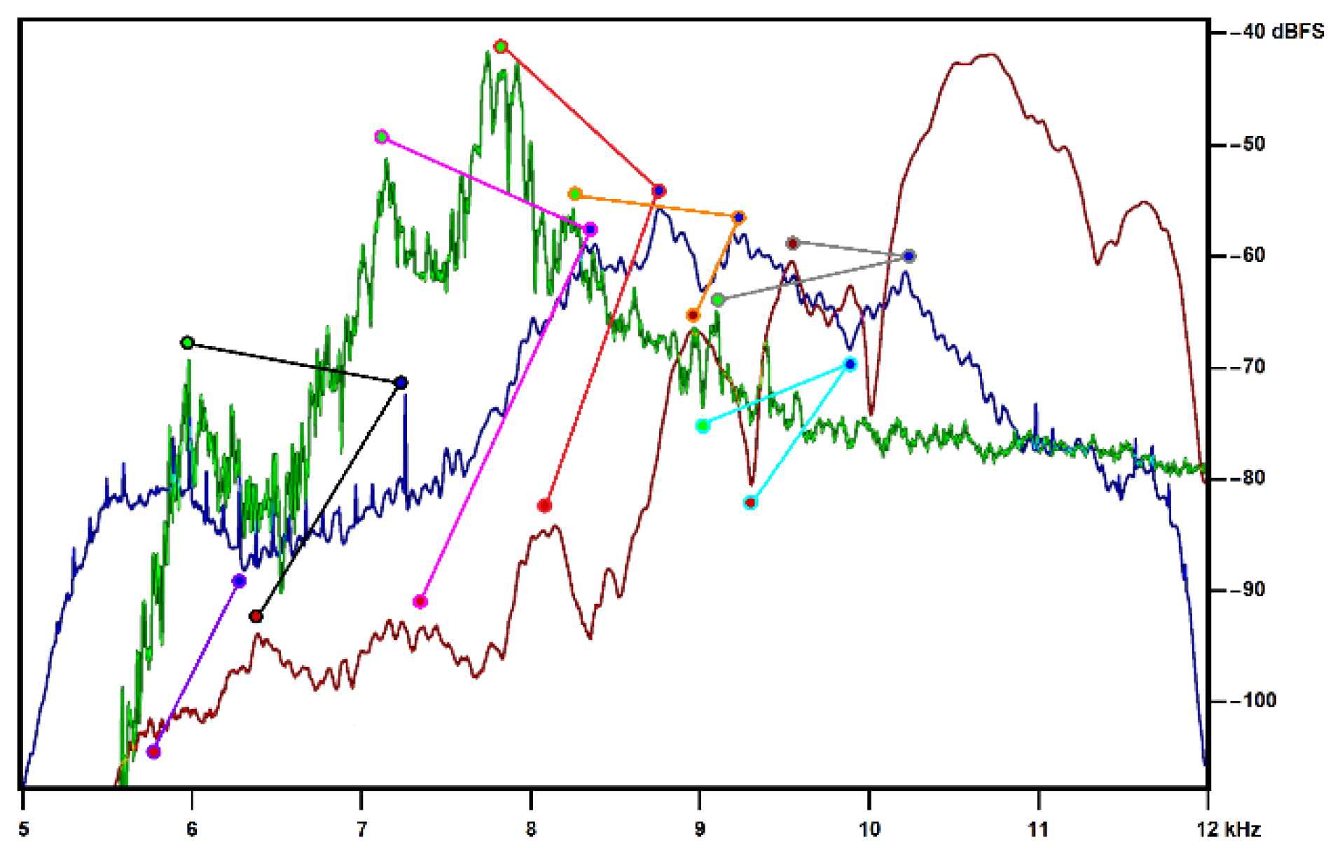
Figure 2.
HTML file with a table containing clickable previews of TAE from the songs by Massa et al. (2012) made for personal use by author CB.
Figure 2.
HTML file with a table containing clickable previews of TAE from the songs by Massa et al. (2012) made for personal use by author CB.
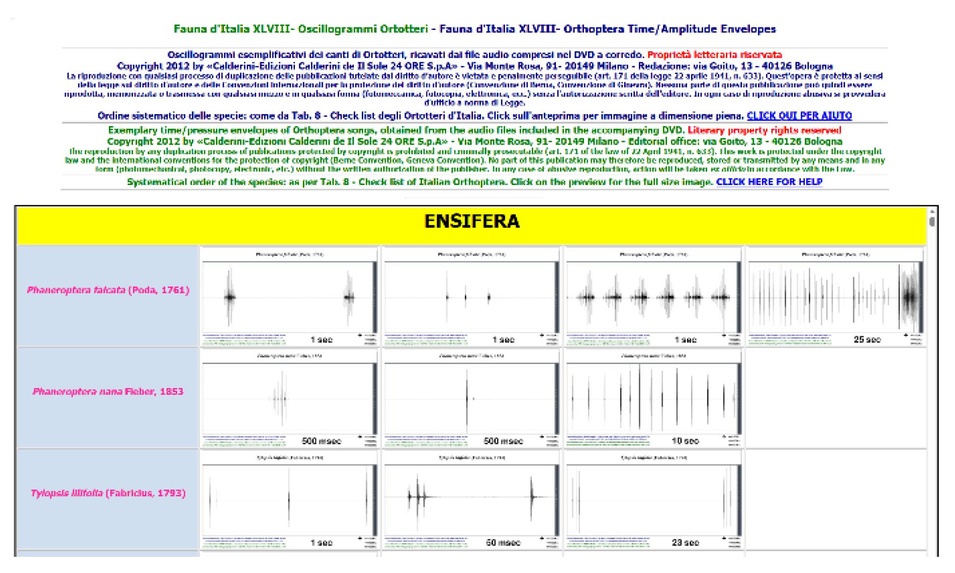
Figure 3.
“The Sandwich Method”. From the reference CD or form the online repository, a recording of candidate species 123 is selected for the current comparison. On-screen TAE is zoomed to a short time interval, bordered in green and dubbed “the bread”. An interval from the novel recording (question mark), half the duration of the bread (“the filling”, bordered in red), is selected and inserted at the center of the bread, thus creating “the sandwich”. A visual comparison of the resulting TAE is performed on screen: if promising, the sandwich is listened to, at slowed-down speed if it engages the inaudible range. The sandwich is saved in a special folder as a screenshot of its TAE and as a new wav file. Actual filenames shall include the shortened versions of the species name, of the reference source and of the locality name, date and time of the novel recording. See the text for exhaustive explanations.
Figure 3.
“The Sandwich Method”. From the reference CD or form the online repository, a recording of candidate species 123 is selected for the current comparison. On-screen TAE is zoomed to a short time interval, bordered in green and dubbed “the bread”. An interval from the novel recording (question mark), half the duration of the bread (“the filling”, bordered in red), is selected and inserted at the center of the bread, thus creating “the sandwich”. A visual comparison of the resulting TAE is performed on screen: if promising, the sandwich is listened to, at slowed-down speed if it engages the inaudible range. The sandwich is saved in a special folder as a screenshot of its TAE and as a new wav file. Actual filenames shall include the shortened versions of the species name, of the reference source and of the locality name, date and time of the novel recording. See the text for exhaustive explanations.
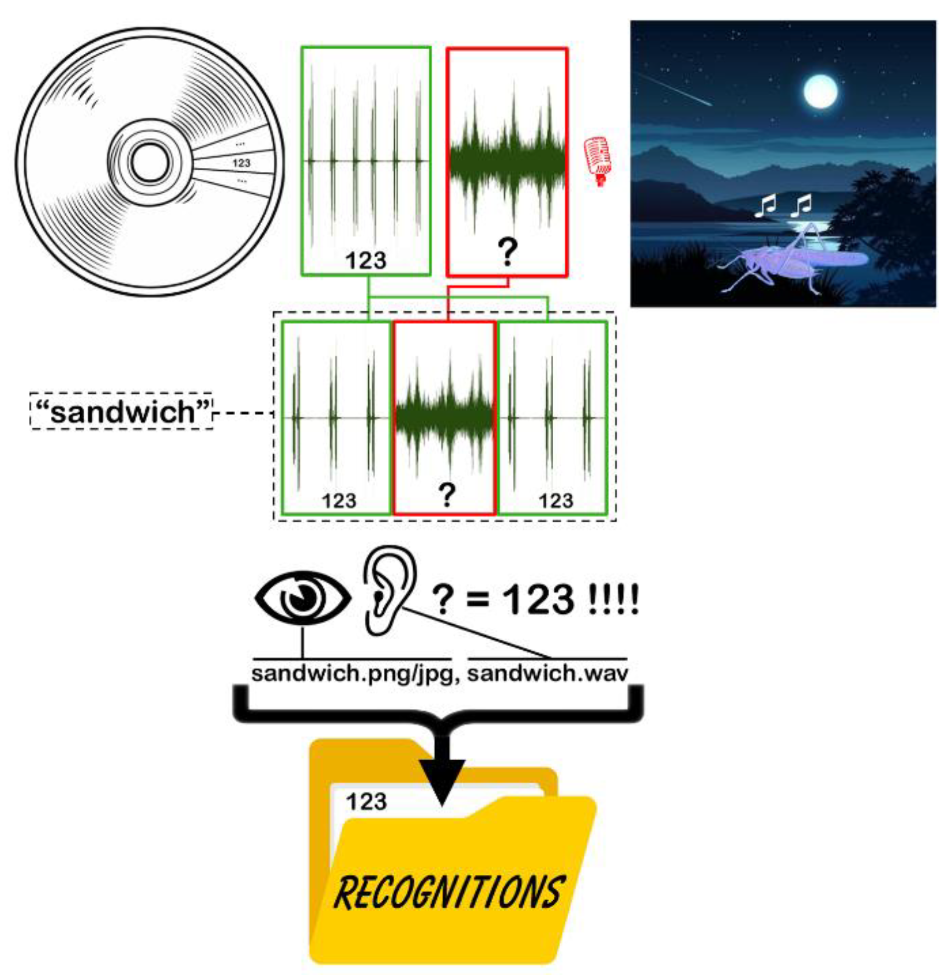
Figure 4.
On-the-fly resampling of the filling during sandwich assembly, examples from three different software. A: Syntrillium Cool Edit Pro and Adobe Audition 1 - the 384 kHz filling - previously copied via Ctrl-c from the novel recording - is pasted via simple Ctrl-v at the center of the bread (reference recording), and is automatically downsampled to the sampling rate of the bread, 44.1 kHz. B: Audacity - operates exactly as illustrated in A. C: Rthoptera Desk, “Merge” Tab - several options are available, including a dropdown list, “sample rate”; according to the sampling rate of the bread (in this case, 44.1 kHz, lower than that of the filling, 384 kHz) the “resample to the lowest” option is selected; the “Merge” button creates the sandwich that can subsequently be exported in wav format.
Figure 4.
On-the-fly resampling of the filling during sandwich assembly, examples from three different software. A: Syntrillium Cool Edit Pro and Adobe Audition 1 - the 384 kHz filling - previously copied via Ctrl-c from the novel recording - is pasted via simple Ctrl-v at the center of the bread (reference recording), and is automatically downsampled to the sampling rate of the bread, 44.1 kHz. B: Audacity - operates exactly as illustrated in A. C: Rthoptera Desk, “Merge” Tab - several options are available, including a dropdown list, “sample rate”; according to the sampling rate of the bread (in this case, 44.1 kHz, lower than that of the filling, 384 kHz) the “resample to the lowest” option is selected; the “Merge” button creates the sandwich that can subsequently be exported in wav format.
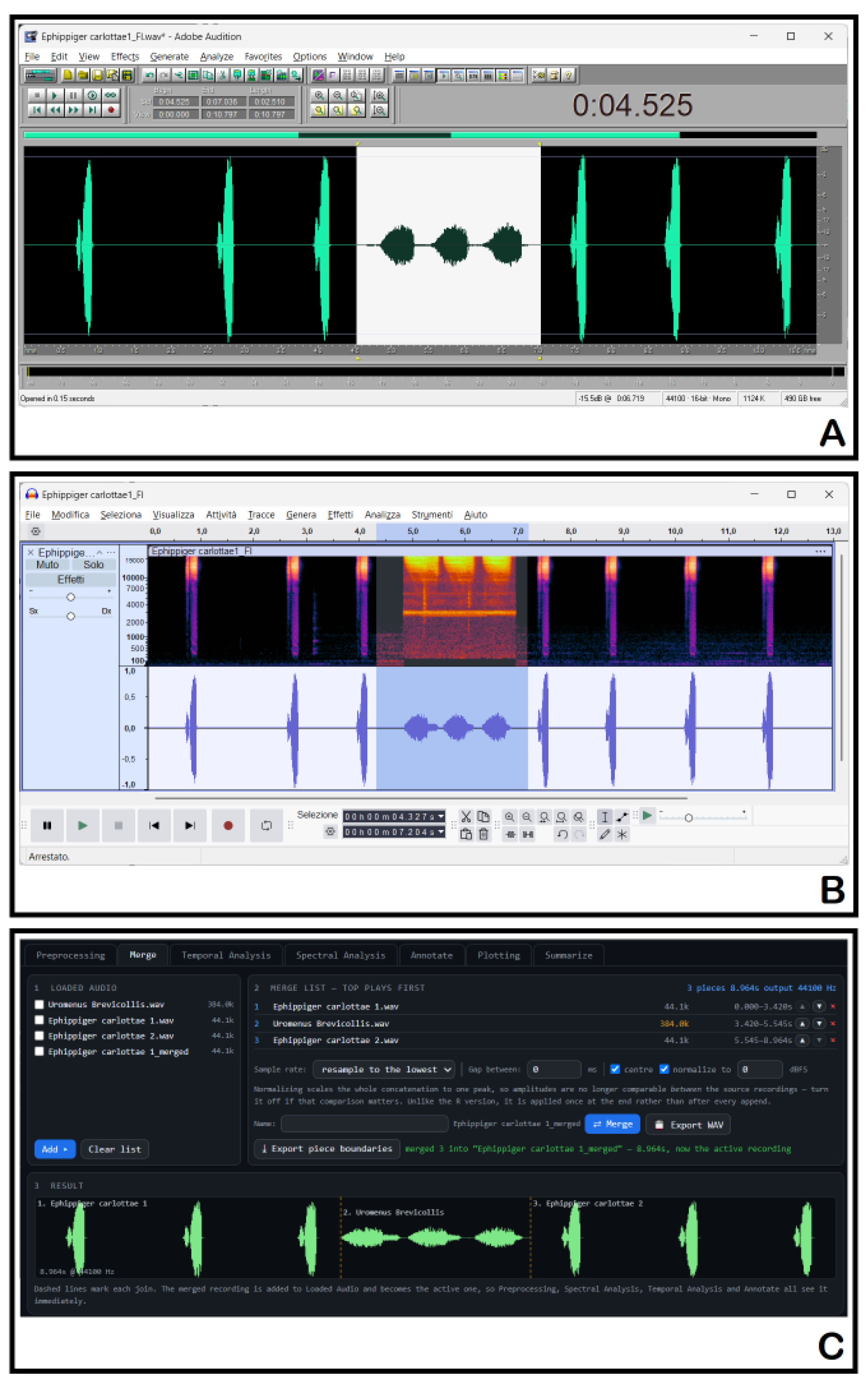
Figure 5.
(From Brizio et al., 2024). Workflow for species recognition from multi-species Passive Acoustic Monitoring recordings. SAS = “Surviving Acoustic Signature”; RAS = “Reference Audio Sample” (here, “Reference Recording”). Other acronyms as in the text.
Figure 5.
(From Brizio et al., 2024). Workflow for species recognition from multi-species Passive Acoustic Monitoring recordings. SAS = “Surviving Acoustic Signature”; RAS = “Reference Audio Sample” (here, “Reference Recording”). Other acronyms as in the text.
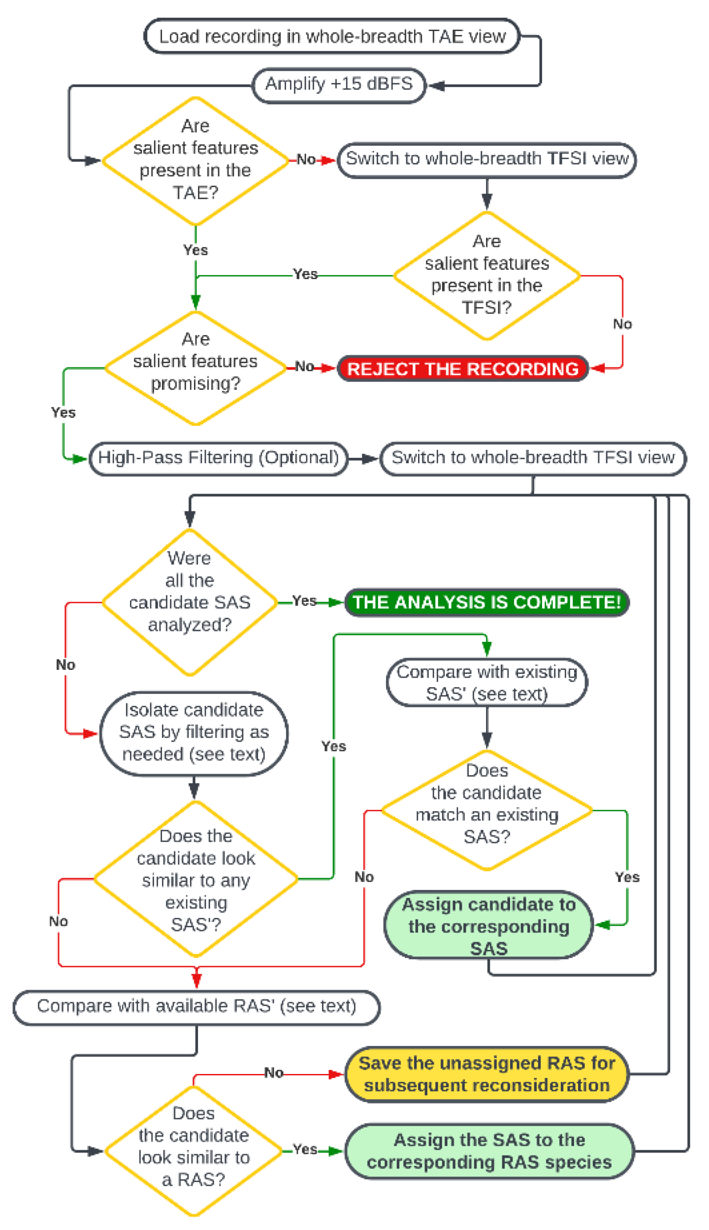
Figure 6.
(Modified from Brizio & Buzzetti, 2014). Flowchart of the high-pass filtering and amplification method that may allow a successful comparison between a recording obtained with a wide-band microphone, unresponsive in the audible range, and a reference recording covering just the audible band. “Ultramic” refers to the namesake microphone by Dodotronic, but epitomizes any microphone capable of recording frequencies in the ultrasonic range. See the text and Brizio & Buzzetti (2014) for further explanations.
Figure 6.
(Modified from Brizio & Buzzetti, 2014). Flowchart of the high-pass filtering and amplification method that may allow a successful comparison between a recording obtained with a wide-band microphone, unresponsive in the audible range, and a reference recording covering just the audible band. “Ultramic” refers to the namesake microphone by Dodotronic, but epitomizes any microphone capable of recording frequencies in the ultrasonic range. See the text and Brizio & Buzzetti (2014) for further explanations.
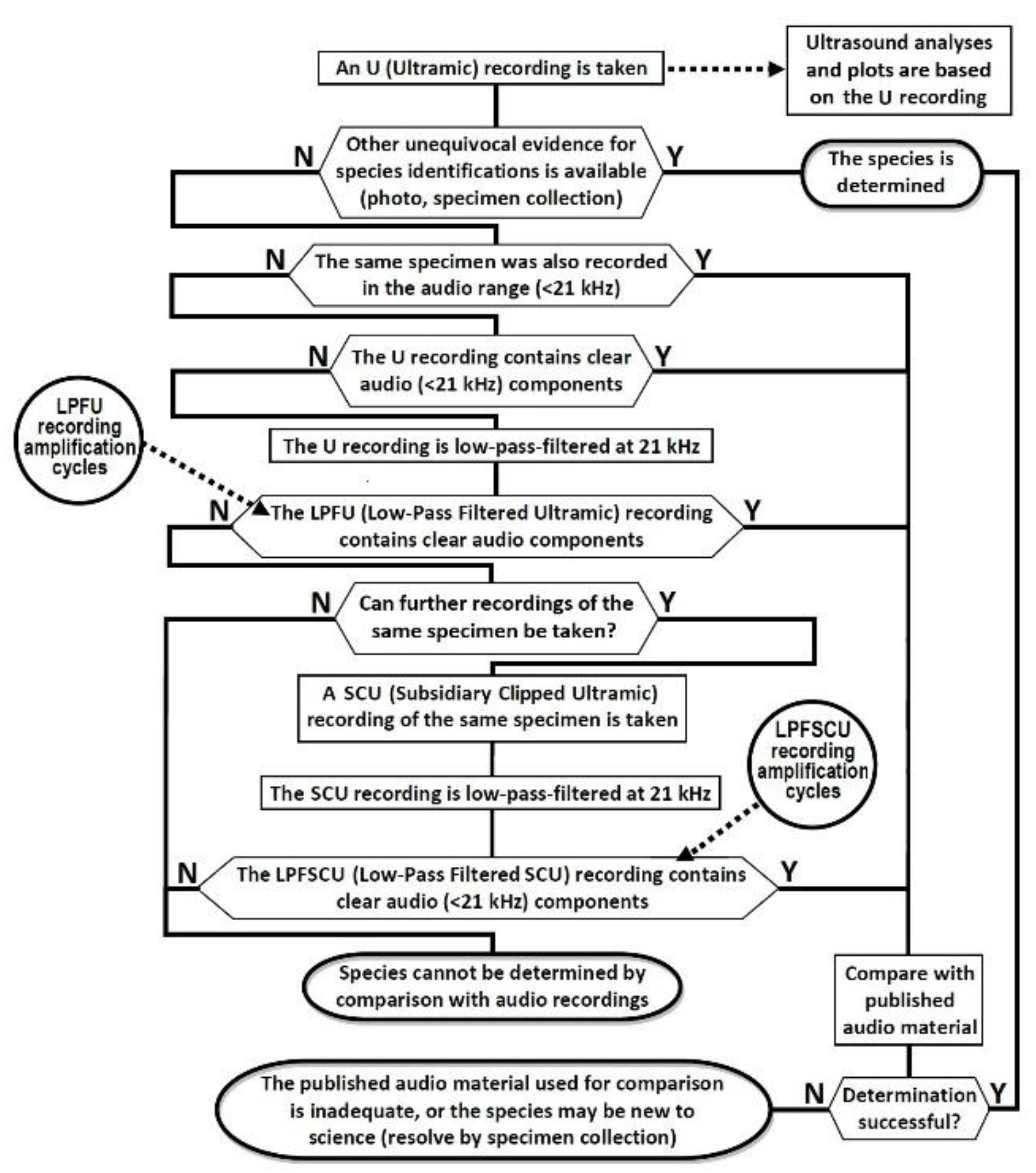
Figure 7.
(From a YouTube video by W. Forstmeier, with permission by the author). Time/Amplitude Envelopes of four songs of P. parallelus at increasing reported air temperature, showing a relevant decrease of echeme duration. The temperature of the insect may vary depending from its position (direct sunlight or shadow). The approximate temperatures at the insect position are inductively indicated in red.
Figure 7.
(From a YouTube video by W. Forstmeier, with permission by the author). Time/Amplitude Envelopes of four songs of P. parallelus at increasing reported air temperature, showing a relevant decrease of echeme duration. The temperature of the insect may vary depending from its position (direct sunlight or shadow). The approximate temperatures at the insect position are inductively indicated in red.
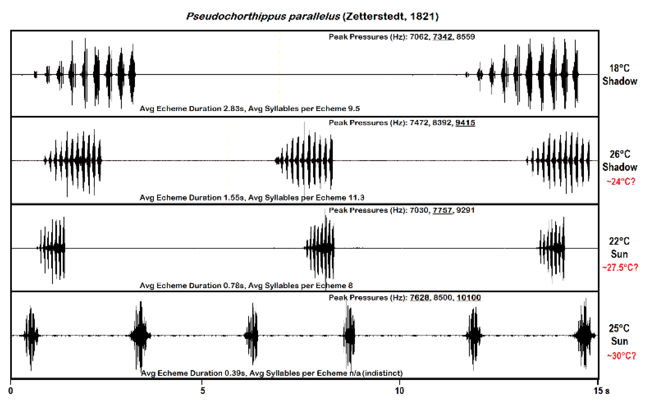
Figure 8.
Detail from the longest and from the shortest echeme in Figure 6. In the latter, syllables coalesce and the typical structure of the echeme is barely evident.
Figure 8.
Detail from the longest and from the shortest echeme in Figure 6. In the latter, syllables coalesce and the typical structure of the echeme is barely evident.
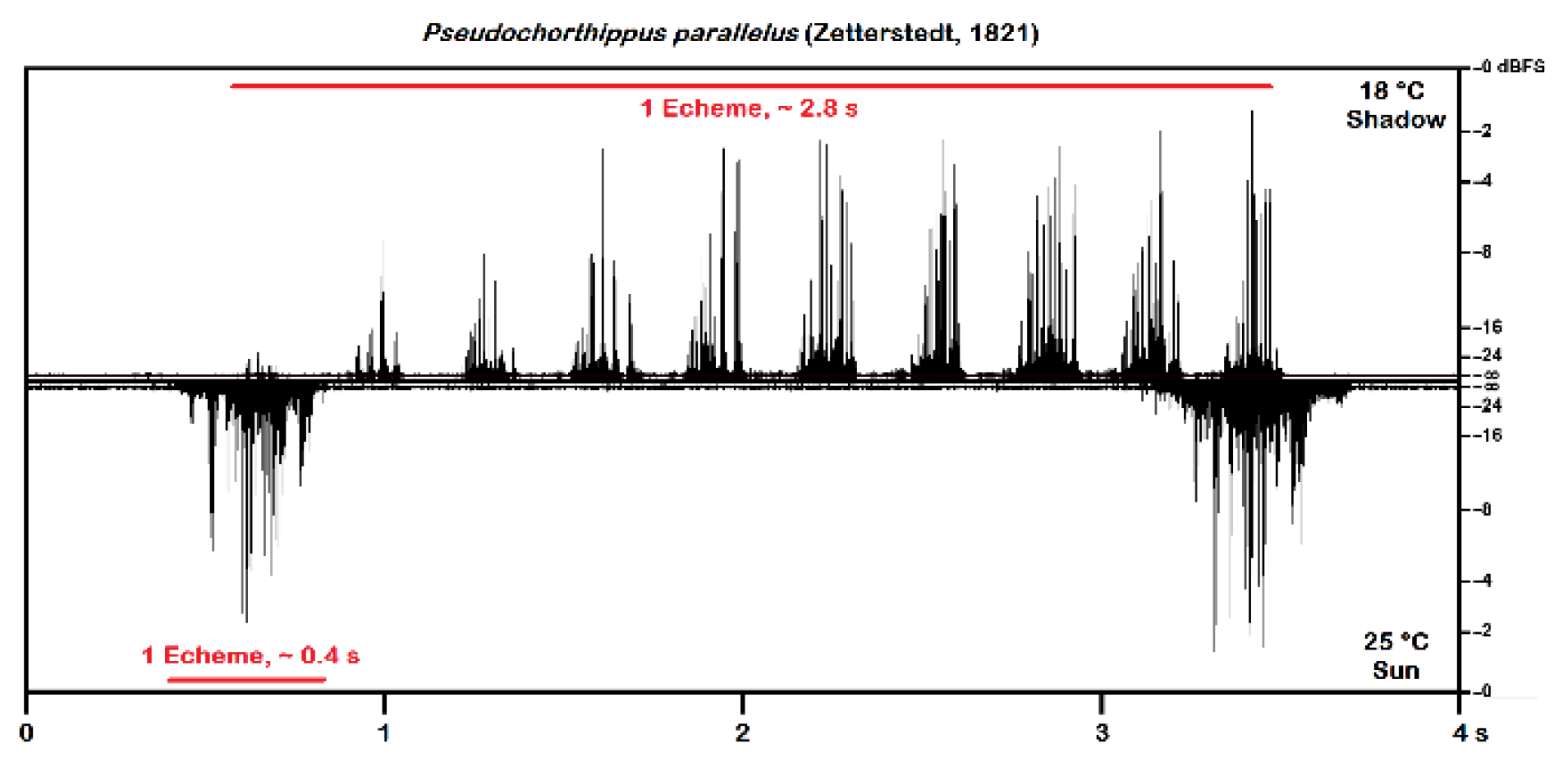
Figure 9.
Cyrtaspis scutata (Charpentier, 1825), spectrograms (0–60 kHz window) and TAE’s of two seconds of calling song. A,B: Massa et al., 2012, sampling frequency 44.1 kHz, recorded band 0–22.05 kHz, apparent echeme duration 3 ms; C,D: author CB, sampling frequency 384 kHz, 29 April 2026 22:40 in Fluminimaggiore (Sardinia) estimated air temperature 16 °C, actual echeme duration around 75 ms; E, F: author CB, sampling frequency 384 kHz, 20 April 2024 in Cereglio (Emilia Romagna), estimated air temperature 12 °C, actual echeme duration up to 125 ms. The red frame in the spectrogram shows the frequency range corresponding with that in A. The blue frames in the TPE’s enclose the only part of each echeme that emerges under the 22.05 kHz threshold, and explain the disproportionately lower apparent duration of the echemes in B.
Figure 9.
Cyrtaspis scutata (Charpentier, 1825), spectrograms (0–60 kHz window) and TAE’s of two seconds of calling song. A,B: Massa et al., 2012, sampling frequency 44.1 kHz, recorded band 0–22.05 kHz, apparent echeme duration 3 ms; C,D: author CB, sampling frequency 384 kHz, 29 April 2026 22:40 in Fluminimaggiore (Sardinia) estimated air temperature 16 °C, actual echeme duration around 75 ms; E, F: author CB, sampling frequency 384 kHz, 20 April 2024 in Cereglio (Emilia Romagna), estimated air temperature 12 °C, actual echeme duration up to 125 ms. The red frame in the spectrogram shows the frequency range corresponding with that in A. The blue frames in the TPE’s enclose the only part of each echeme that emerges under the 22.05 kHz threshold, and explain the disproportionately lower apparent duration of the echemes in B.
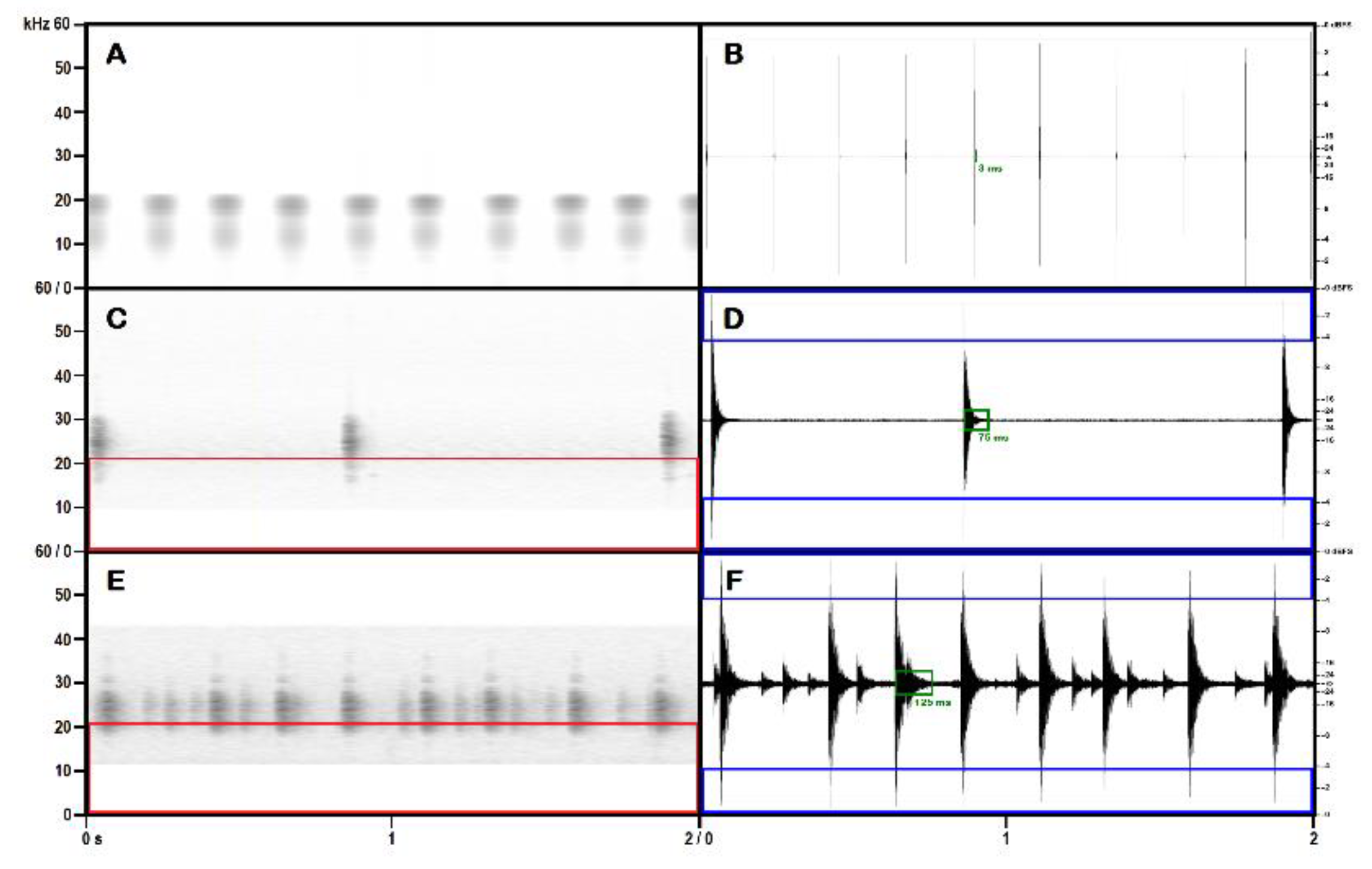
Figure 10.
Comparison of the TAE (audible range) of three echemes emitted at increasing unreported temperatures. Above: Pseudochorthippus parallelus (Zetterstedt, 1821), below Pholidoptera aptera (Fabricius, 1793).
Figure 10.
Comparison of the TAE (audible range) of three echemes emitted at increasing unreported temperatures. Above: Pseudochorthippus parallelus (Zetterstedt, 1821), below Pholidoptera aptera (Fabricius, 1793).
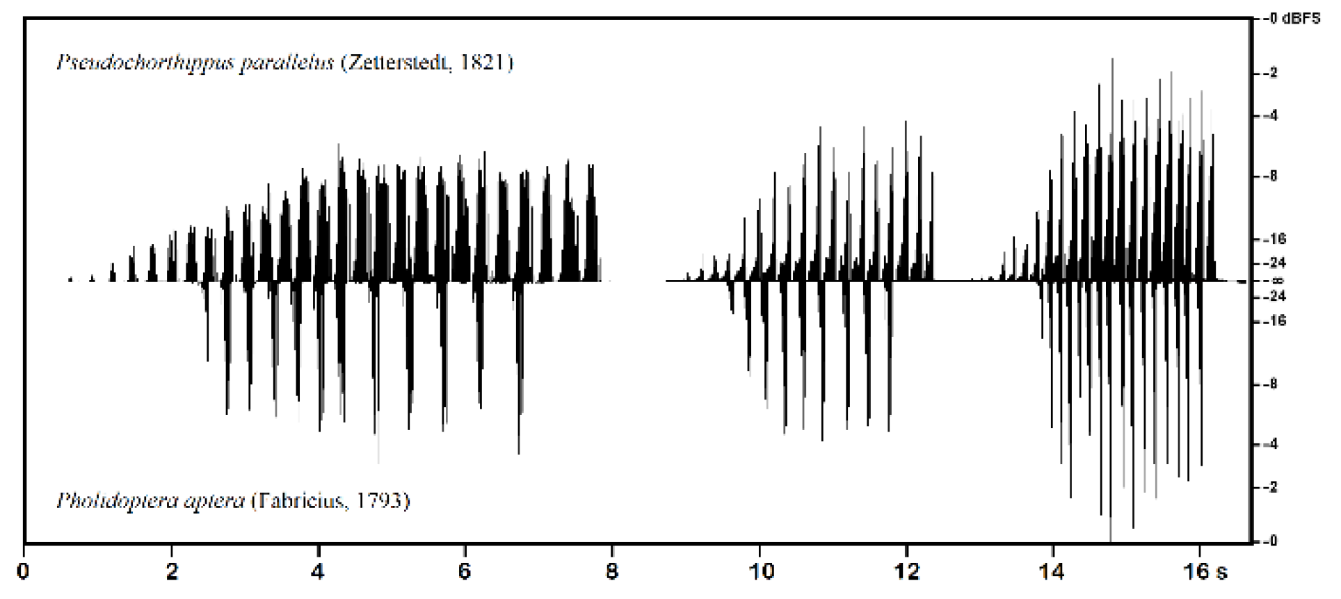
Figure 11.
Comparison of the TAE (audible range) of one second of the song. Above: Pseudochorthippus parallelus (Zetterstedt, 1821), below Pholidoptera aptera (Fabricius, 1793).
Figure 11.
Comparison of the TAE (audible range) of one second of the song. Above: Pseudochorthippus parallelus (Zetterstedt, 1821), below Pholidoptera aptera (Fabricius, 1793).
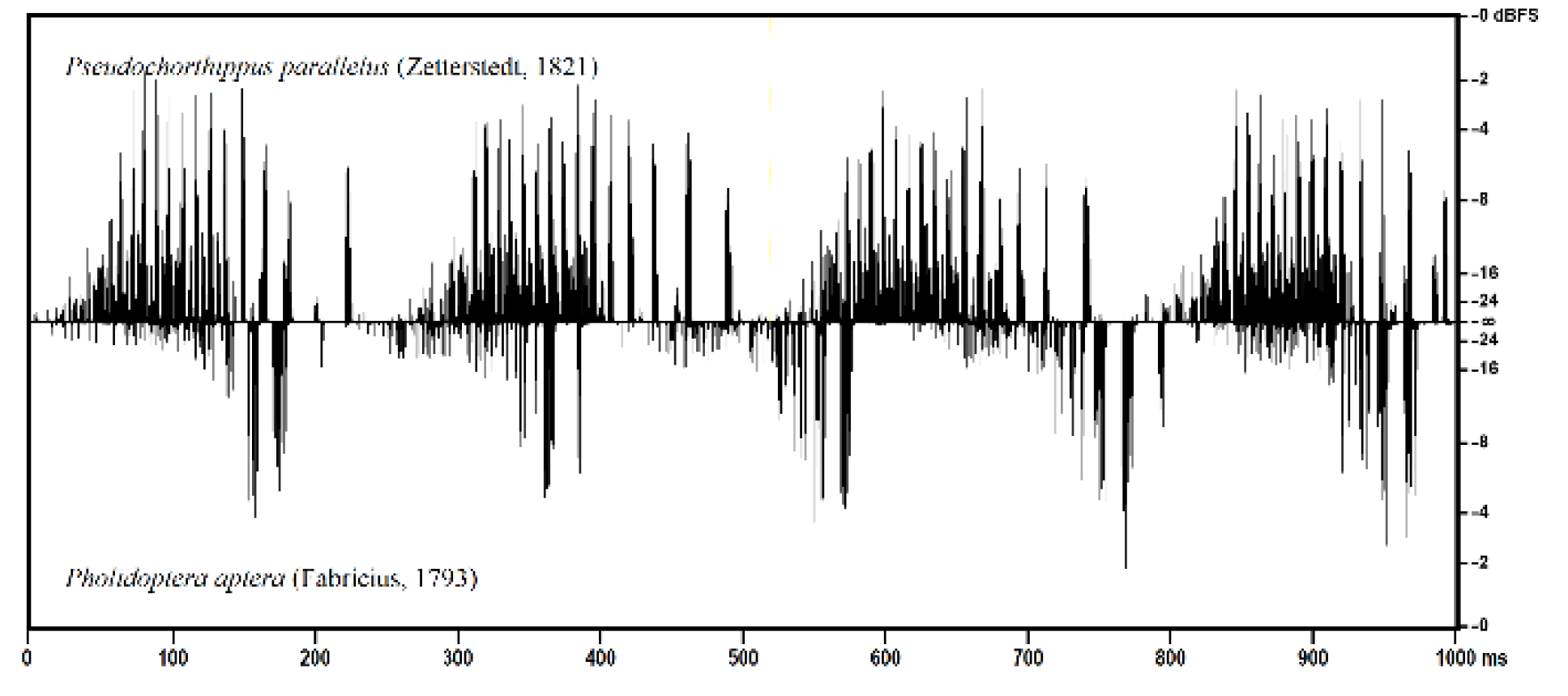
Figure 12.
Comparison of the spectrogram (audible range) of three echemes emitted at increasing unreported temperatures. Above: Pseudochorthippus parallelus (Zetterstedt, 1821), below Pholidoptera aptera (Fabricius, 1793). Mean Spectra (black area) are superposed to the left portion of the spectrogram. Diagnostic features are indicated by a caption.
Figure 12.
Comparison of the spectrogram (audible range) of three echemes emitted at increasing unreported temperatures. Above: Pseudochorthippus parallelus (Zetterstedt, 1821), below Pholidoptera aptera (Fabricius, 1793). Mean Spectra (black area) are superposed to the left portion of the spectrogram. Diagnostic features are indicated by a caption.
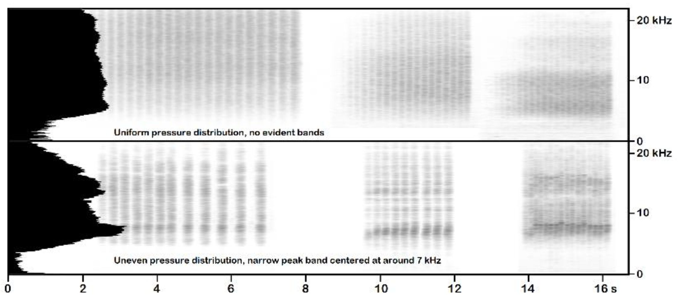
Figure 13.
Comparison of the TAE (audible range) of around sixteen seconds of the song. Above: Omocestus haemorrhoidalis (Charpentier, 1825), below Tettigonia cantans (Fuessly, 1775).
Figure 13.
Comparison of the TAE (audible range) of around sixteen seconds of the song. Above: Omocestus haemorrhoidalis (Charpentier, 1825), below Tettigonia cantans (Fuessly, 1775).
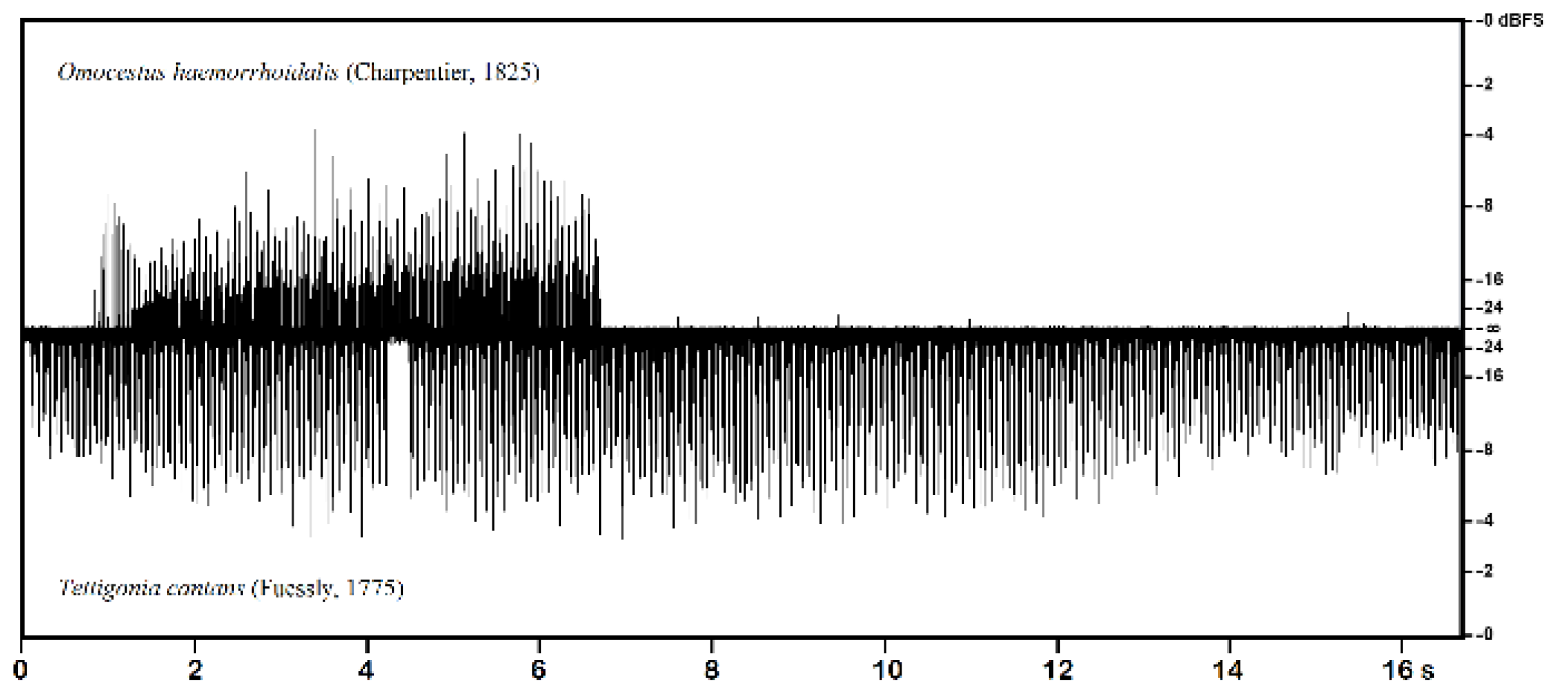
Figure 14.
Comparison of the TAE (audible range) of around a dozen syllables emitted in one second. Above: Omocestus haemorrhoidalis (Charpentier, 1825), below Tettigonia cantans (Fuessly, 1775).
Figure 14.
Comparison of the TAE (audible range) of around a dozen syllables emitted in one second. Above: Omocestus haemorrhoidalis (Charpentier, 1825), below Tettigonia cantans (Fuessly, 1775).
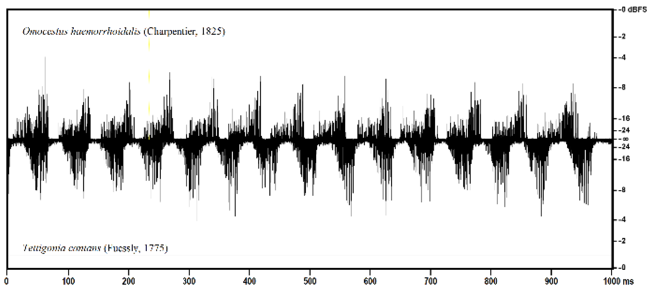
Figure 15.
Comparison of the spectrogram (audible range) of three echemes emitted at increasing unreported temperatures. Above: Omocestus haemorrhoidalis (Charpentier, 1825), below Tettigonia cantans (Fuessly, 1775). Mean Spectra (black area) are superposed to the left portion of the spectrogram. Diagnostic features are indicated by arrows and captions.
Figure 15.
Comparison of the spectrogram (audible range) of three echemes emitted at increasing unreported temperatures. Above: Omocestus haemorrhoidalis (Charpentier, 1825), below Tettigonia cantans (Fuessly, 1775). Mean Spectra (black area) are superposed to the left portion of the spectrogram. Diagnostic features are indicated by arrows and captions.
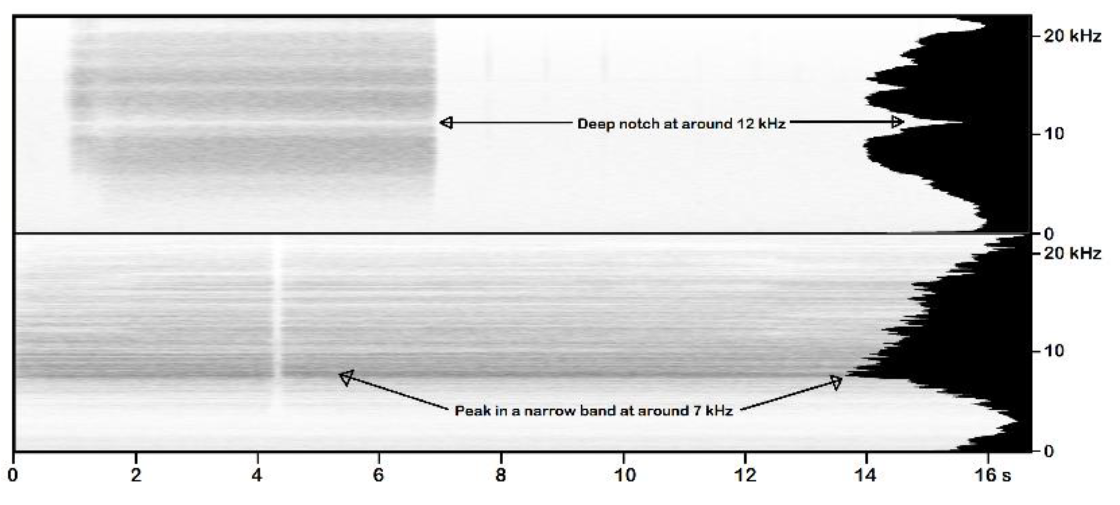
Figure 16.
TAE of a mosaic of five echemes (50 ms each) from the songs of, from left to right, Cyrtaspis scutata (Charpentier, 1825), Leptophyes laticauda (Fridvalsky, 1867), Poecilimon ornatus (Schmidt, 1850), Tylopsis lilifolia (Fabricius, 1793), Yersinella raymondii (Yersin, 1860) recorded in the audible range. The mosaic is used to compare an unknown short-duration echeme with that of the five species considered, as illustrated in the text. From the recordings in the accompanying DVD of Massa et al. (2012).
Figure 16.
TAE of a mosaic of five echemes (50 ms each) from the songs of, from left to right, Cyrtaspis scutata (Charpentier, 1825), Leptophyes laticauda (Fridvalsky, 1867), Poecilimon ornatus (Schmidt, 1850), Tylopsis lilifolia (Fabricius, 1793), Yersinella raymondii (Yersin, 1860) recorded in the audible range. The mosaic is used to compare an unknown short-duration echeme with that of the five species considered, as illustrated in the text. From the recordings in the accompanying DVD of Massa et al. (2012).
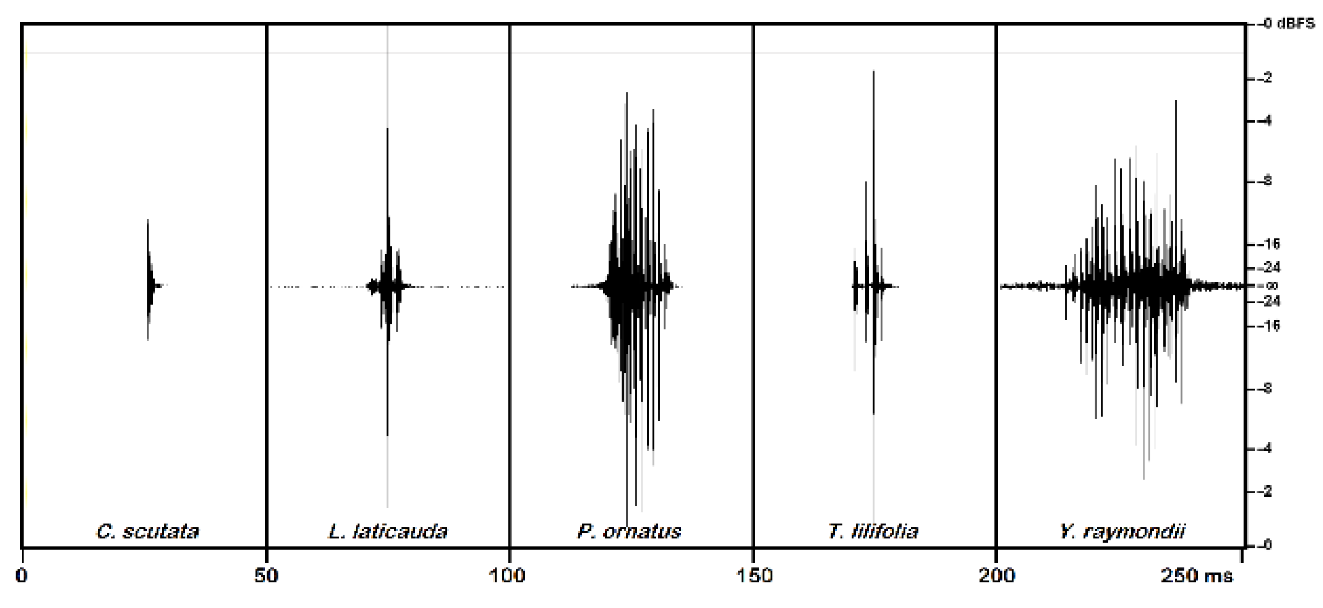
Figure 17.
Spectrogram of the mosaic in Figure 15. The abrupt truncation of the frequency patterns at 21 kHz reveals relevant spectral energy in the inaudible range. From the recordings in the accompanying DVD of Massa et al. (2012).
Figure 17.
Spectrogram of the mosaic in Figure 15. The abrupt truncation of the frequency patterns at 21 kHz reveals relevant spectral energy in the inaudible range. From the recordings in the accompanying DVD of Massa et al. (2012).
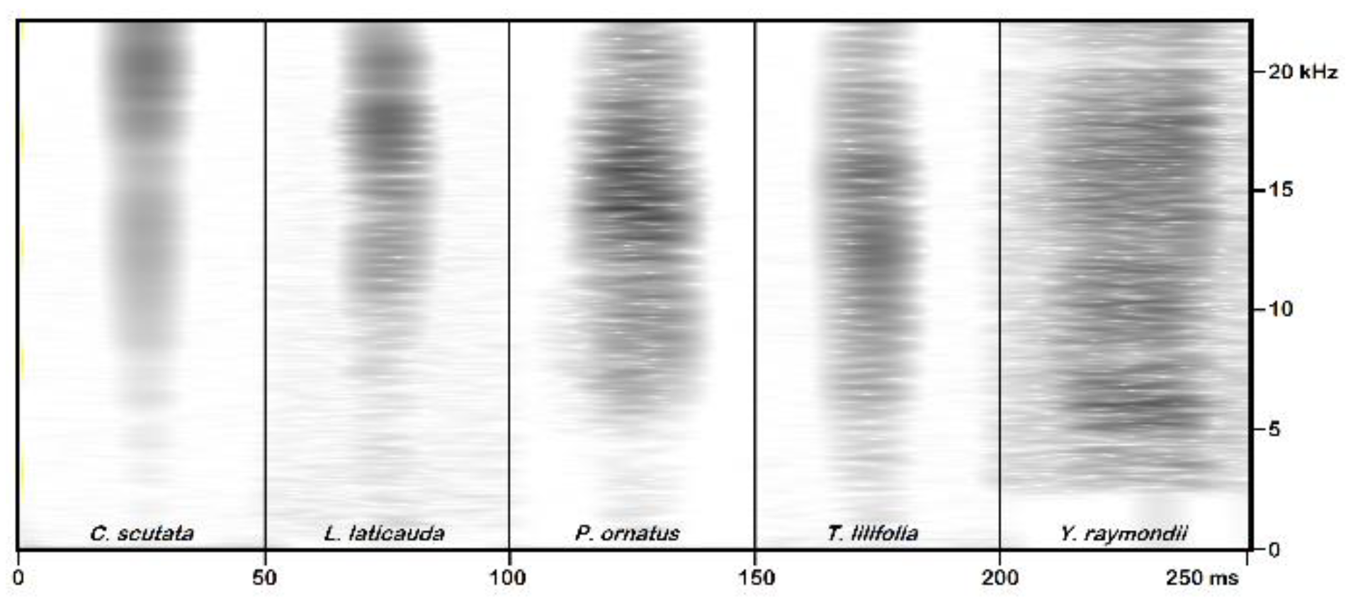
Figure 18.
Rhacocleis germanica (Herrich-Schäffer, 1840), procedure of recognition of the song by the sandwich method. Details are provided in the text. A, B: TAE and spectrogram (0-90 kHz) of 16 seconds from the novel recording, unfiltered; C, D: spectrogram and TAE of the novel recording, after filtering; E: selection of a time strip of around 2 seconds (filling); F: selection of a time strip of around 4 seconds from the reference recording (bread); G: sandwich; H: the sandwich during the slowed-down listening phase.
Figure 18.
Rhacocleis germanica (Herrich-Schäffer, 1840), procedure of recognition of the song by the sandwich method. Details are provided in the text. A, B: TAE and spectrogram (0-90 kHz) of 16 seconds from the novel recording, unfiltered; C, D: spectrogram and TAE of the novel recording, after filtering; E: selection of a time strip of around 2 seconds (filling); F: selection of a time strip of around 4 seconds from the reference recording (bread); G: sandwich; H: the sandwich during the slowed-down listening phase.
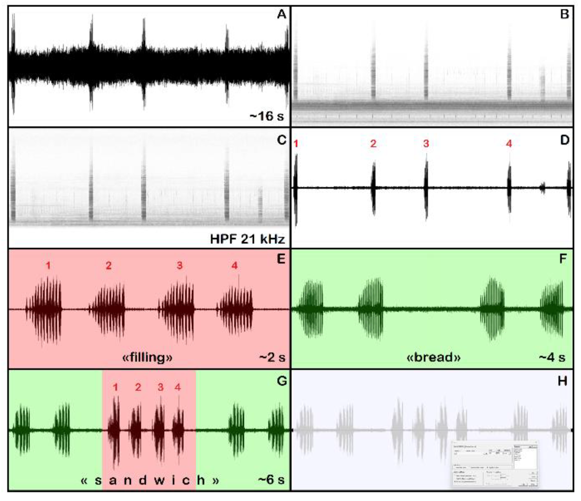
Figure 19.
Conocephalus conocephalus (Linnaeus, 1767), procedure of recognition of the song by the sandwich method. Details are provided in the text. A, B: TAE and spectrogram (0-100 kHz) of 16 seconds from the novel recording, unfiltered; C, D: spectrogram and TAE of the novel recording, after filtering; E: selection of a time strip of around 2 seconds (filling); F: selection of a time strip of around 4 seconds from the reference recording (bread); G: sandwich; H: the sandwich during the slowed-down listening phase.
Figure 19.
Conocephalus conocephalus (Linnaeus, 1767), procedure of recognition of the song by the sandwich method. Details are provided in the text. A, B: TAE and spectrogram (0-100 kHz) of 16 seconds from the novel recording, unfiltered; C, D: spectrogram and TAE of the novel recording, after filtering; E: selection of a time strip of around 2 seconds (filling); F: selection of a time strip of around 4 seconds from the reference recording (bread); G: sandwich; H: the sandwich during the slowed-down listening phase.
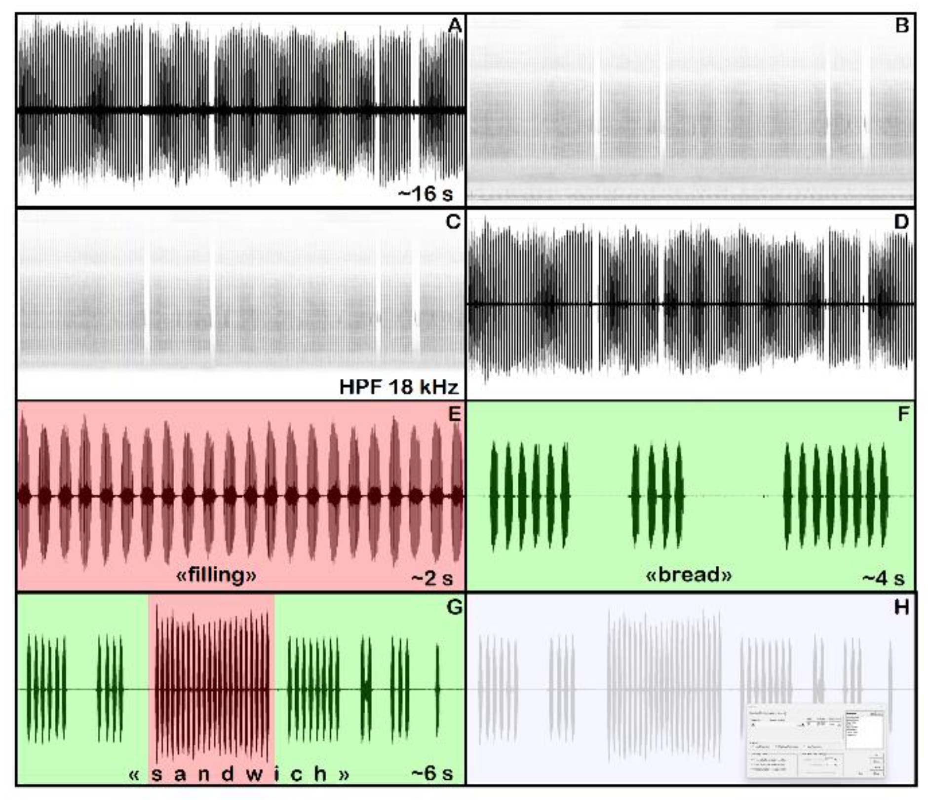
Disclaimer/Publisher’s Note: The statements, opinions and data contained in all publications are solely those of the individual author(s) and contributor(s) and not of MDPI and/or the editor(s). MDPI and/or the editor(s) disclaim responsibility for any injury to people or property resulting from any ideas, methods, instructions or products referred to in the content. |
© 2026 by the authors. Licensee MDPI, Basel, Switzerland. This article is an open access article distributed under the terms and conditions of the Creative Commons Attribution (CC BY) license (http://creativecommons.org/licenses/by/4.0/).
Copyright: This open access article is published under a Creative Commons CC BY 4.0 license, which permit the free download, distribution, and reuse, provided that the author and preprint are cited in any reuse.