

Submitted:
27 August 2026
Posted:
28 August 2026
You are already at the latest version
Abstract
Wing icing alters the aerodynamic shape of lifting surfaces and threatens aviation safety. Image-based semantic segmentation provides spatial information on visible wing-surface icing, yet most existing studies rely on wind-tunnel, bench-test, or simulated images, and image-level random splits overestimate generalization for video-derived data. This study builds a complete workflow from flight-test data collection to onboard prototype verification for wing icing segmentation under real flight conditions. A real UAV flight-test dataset of 13,894 pixel-level annotated images was built from backward-view wing videos over the Qinghai–Tibet Plateau, with flight-wise split as the primary protocol to assess generalization to unseen sorties. To address boundary under-segmentation in early-stage icing, an ROI boundary-weighted loss is introduced, combining ROI spatial masking and boundary pixel weighting, supplemented by optical-flow-guided inter-frame smoothing. Relative to the SENet+CBAM attention baseline, this loss raises Recall in the Rice<3% group by up to 6.03 percentage points in the best single run (mean +2.27 pp over three runs) and reduces inter-frame Dice variance by 71% in the single-run comparison (approximately 51% on three-run means). The final scheme achieves 91.34% Dice and 84.07% IoU (three-run means), and a bench-level prototype evaluation on an embedded GPU platform indicates compute feasibility for a 2 s/frame detection cycle. The primary contributions are a real UAV flight-test benchmark with rigorous flight-wise generalization assessment, an ROI boundary-weighted loss that improves early-stage icing recall relative to the attention baseline and reduces inter-frame prediction variance, and a bench-level onboard prototype evaluation on an embedded GPU platform indicating compute feasibility for a 2 s/frame detection cycle.
Keywords:
wing icing
; semantic segmentation
; unmanned aerial vehicle
; flight-test image
; ROI boundary-weighted loss
; inter-frame smoothing
; prototype validation
1. Introduction
Aircraft icing is one of the major environmental hazards affecting aviation safety. When an aircraft operates in clouds containing supercooled water droplets, ice can rapidly accrete on critical surfaces such as wings, empennages, engine inlets, and sensor probes, forming rime, glaze, or mixed-phase ice. Ice accretion on wings changes the local aerodynamic profile, promotes premature boundary-layer separation, reduces lift, increases drag, and decreases the stall angle of attack, which under severe conditions can lead to stall, loss of control, and accidents. Previous studies have shown that icing effects are particularly pronounced for small unmanned aerial vehicles (UAVs) and high-lift-to-drag-ratio wings, where aerodynamic degradation can markedly compress the flight safety margin [1,2,3,4,5,6]. Timely and accurate detection of wing-surface icing is therefore valuable for icing warning, activation of anti-icing or de-icing systems, and flight-strategy adjustment. The physics of ice accretion on lifting surfaces and the regulatory icing envelopes that define operating conditions are well established [7,8,9,10]; image-based sensing provides a complementary spatial view of the icing state [11].
Traditional aircraft icing detection techniques include electrical, thermal, resonant, optical, and ultrasonic or guided-wave methods [12,13,14,15,16,17]. These sensors can provide local information on icing occurrence, ice thickness, or ice type and have been applied in aviation icing monitoring and anti-icing control. However, most existing sensors are point- or line-wise devices whose readings are highly dependent on the mounting location, and they cannot easily reflect the full spatial distribution of ice on a wing surface. For small and medium-sized UAVs and platforms with limited onboard space, a non-contact, low-cost monitoring method capable of covering a larger wing area is of practical interest.
With recent advances in computer vision and deep learning, image-based wing icing detection has become an active research direction in aviation icing monitoring. Semantic segmentation can provide pixel-level icing region extraction, which is suitable for estimating icing area, icing boundaries, and the time evolution of ice growth. Classical image processing, U-Net, DeepLab-series models, Transformer-based segmentation networks, and lightweight convolutional networks have been progressively applied to wing icing image recognition [18,19,20,21,22,23,24,25,26,27,28,29,30,31], and attention mechanisms have been used to enhance icing-relevant features in the channel or spatial dimensions [32,33,34].
Although published studies have demonstrated the feasibility of deep learning for wing icing image recognition, a gap remains between these studies and engineering application under real flight conditions. Most existing image datasets come from ice wind tunnels, bench tests, or simulated environments, and they cover real flight challenges such as cloud background, specular reflection, exposure variation, camera vibration, and viewpoint differences to a limited extent. In addition, many studies still report results based on image-level random splits or single-dataset accuracy, which may not adequately reflect a model’s generalization to unseen flight sorties. For weak-signal scenarios such as early-stage icing, small ice crystals, and transparent thin ice, relying solely on single-frame texture features can lead to missed detection and boundary instability. Hence, the spatial priors derived from a fixed camera view, and the temporal continuity present in flight video sequences, remain underexploited.
In preliminary experiments conducted for this study, the Dice score exceeded 95% under image-level random splitting, but dropped to approximately 91% under flight-wise splitting. A key methodological concern in video-derived datasets is that image-level random splitting allows correlated adjacent frames from the same sortie to appear in both training and test sets, leading to optimistic accuracy estimates; in the preliminary experiments this inflation reached 4–5 percentage points. This paper therefore advocates flight-wise splitting as the standard evaluation protocol for sortie-derived icing image datasets, and centers the method design and prototype verification around two practical problems: boundary under-segmentation in early-stage icing, and inter-frame prediction fluctuation in video sequences.
This work focuses on constructing and rigorously evaluating a complete engineering workflow for flight-test wing icing segmentation, addressing the gap between wind-tunnel studies and operational deployment. The main contributions are as follows.
- 1.
- A real UAV flight-test wing icing segmentation dataset containing 13,894 pixel-level annotated images is constructed, and a flight-wise split is adopted to evaluate generalization to unseen sorties, with image-level random split results reported only as an in-distribution reference.
- 2.
- A wing-surface ROI boundary-weighted loss is introduced to exploit fixed-camera-view spatial priors. Decomposition into ROI-masking and boundary-weighting components reveals complementary roles: the former suppresses wing-exterior false alarms, while the latter improves recall by up to 6.03 percentage points on early-stage icing samples () in the best single run compared with the SENet+CBAM baseline (mean +2.27 pp over three runs) and reduces inter-frame Dice variance by 71% in the single-run comparison with the same baseline (approximately 51% on three-run means).
- 3.
- Optical-flow-guided inter-frame smoothing is integrated as a post-processing module for additional prediction stability, and a prototype verification is conducted on an MIC-770V3 onboard embedded platform (RTX A2000 Embedded 8 GB) to assess runtime and resource feasibility toward onboard deployment.
The remainder of this paper is organized as follows. Section 2 describes the flight-test data acquisition, dataset construction, annotation procedure, and the segmentation methodology. Section 3 reports the experimental results and analysis, including onboard deployment verification. Section 4 provides a discussion of module contributions, generalization, engineering implications, and limitations. Section 5 summarizes the conclusions, and Appendix A reports the image-level random split results as an in-distribution reference.
2. Materials and Methods
2.1. UAV Platform and Camera Configuration
The flight-test data were collected using a Tengdun Twin-Tailed Scorpion A large fixed-wing UAV as the experimental platform. A GoPro HERO11 Black camera was mounted near the engine nacelle with a fixed backward view to observe the wing leading edge and upper wing surface. The backward-facing orientation reduces the risk of supercooled water droplet impingement and icing contamination directly on the camera lens, thereby improving recording stability.
2.2. Flight-Test Region and Environmental Conditions
The flight data were collected over the Qinghai–Tibet Plateau from July to November 2024. This region is characterized by high altitude, low temperature, high humidity, and complex cloud layer distribution. A total of 35 sorties were completed, yielding 106 h of raw flight video. Approximately 39 h of video correspond to flight segments under icing or potentially icing conditions. The flight-test conditions are summarized in Table 2. Representative flight wing icing images covering eight typical scenarios are shown in Figure 2.
2.3. Raw Video Screening
The raw flight videos contain diverse segments including normal cruise, cloud penetration, ice growth, cloud occlusion, strong illumination, camera vibration, and exposure anomalies. To ensure the quality of the subsequent dataset, manual screening was first performed to exclude segments in which the wing surface was invisible, the lens was severely occluded, prolonged overexposure or underexposure occurred, strong vibration made the wing boundary unrecognizable, the flight was under non-icing cruise conditions, or the timestamp or video file was abnormal.
2.4. Frame Extraction and Preprocessing
After screening, image frames were extracted from the valid icing videos at a fixed interval of 10 s. Manual review was performed to remove frames with motion blur, exposure anomaly, or unclear wing-surface boundary. The final dataset comprises 13,894 valid images with visible wing-surface icing features. All images were resized to 512 × 512 pixels for training, using bilinear interpolation for images and nearest-neighbor interpolation for masks.
Relationship between 10 s and 2 s sampling. Training and single-frame segmentation evaluation were both performed on the 10 s interval annotated images. However, optical flow cannot be reliably computed at a 10 s interval (approximately 240 frames). For inter-frame smoothing evaluation (see Section 2.14 and Section 3.5), dense frames were extracted at a 2 s interval from the original test sortie videos for model inference—an interval consistent with the planned 2 s/frame onboard detection cycle. These dense frames are used for optical flow computation and inter-frame smoothing; Dice, IoU, and are computed only on frames with ground-truth (GT) annotations or at timestamps matching the 10 s annotation frames. Unannotated intermediate frames do not directly participate in these quantitative statistics. This design allows inter-frame smoothing to be evaluated at a reasonable frame interval without incurring additional annotation cost.
2.5. Wing-Surface ROI Definition
Since the raw images contain not only the wing surface but also background regions such as sky, cloud, engine nacelle, and fuselage structures, and given the fixed camera mounting and stable field of view, a fixed wing-surface ROI was manually defined from the training set. The ROI is used for metric calculation (Dice, IoU, ice-area ratio estimation) and as the spatial reference for the boundary-weighted loss. The ROI is defined as a binary mask , where denotes a valid wing-surface pixel. During loss computation and evaluation, the ROI mask constrains Dice, IoU, and ice-area statistics to the valid wing-surface region, preventing non-wing regions such as sky and cloud from interfering with the metrics. The model is still trained with full images as input to retain contextual information surrounding the wing.
2.6. Pixel-Level Annotation and Quality Control
Pixel-level annotations were generated using the ISAT-SAM tool based on Meta’s open-source Segment Anything Model 2 (SAM2). The workflow comprised three stages: manual labeling of key frames, semi-automatic temporal propagation, and manual refinement. Approximately 10% of the frames were labeled manually; the remaining frames were annotated through SAM2 temporal propagation combined with ISAT interactive correction. Annotation results were stored as binary masks.
A two-person cross-checking and manual review procedure was applied for quality control. After the initial annotation, a second annotator reviewed the ice boundaries, transparent thin-ice regions, and areas with strong specular reflection. For samples with inter-annotator disagreement, the two annotators jointly reviewed the original video context to determine the final mask. For regions with uncertain boundaries, the annotation principle was to label only visible, contiguous suspected ice regions and to avoid mislabeling cloud, specular highlight, and wing-surface texture as ice. The annotation statistics are summarized in Table 3.
2.7. Flight-Wise Dataset Split
A flight-wise split was adopted as the primary evaluation protocol, treating the sortie identifier (flight date/sortie number) as the smallest independent partition unit. Among the 22 annotated sorties, 16 were allocated for training, 3 for validation, and 3 for testing. An image-level random split is reported only as an in-distribution reference in Appendix A.
The minimal metadata fields for each sample are listed in Table 4.
2.8. Class Imbalance
Since the icing region typically occupies only a fraction of the image or wing-surface ROI, the dataset exhibits significant foreground–background class imbalance. In addition to pixel accuracy, emphasis is placed on Dice, IoU, recall, and precision as evaluation metrics.
2.9. Baseline Segmentation Models
Four representative segmentation architectures with different context-modeling strategies were evaluated: U-Net [29] (encoder–decoder with skip connections), DeepLabV3+ [30] (atrous convolution with ASPP), Mask2Former [31] (Transformer with masked attention), and SegFormer-B0 [20] (lightweight hierarchical Transformer, 3.71M parameters), which was included as a lightweight Transformer reference. FCN [18], PSPNet [19], and lightweight real-time alternatives [21,22,23] represent additional architectural directions.
All models take an RGB image as input and output an icing probability map , which is binarized with a threshold during inference. Training configurations for the four baseline models are summarized in Table 5.
Note. All models in Table 11 were trained from scratch. U-Net, DeepLabV3+, and SegFormer-B0 share the same PyTorch-native framework and hyperparameter settings. Mask2Former uses the Detectron2 framework with its own training recipe, including longer training iterations, WarmupPolyLR, and multi-scale training, because it requires a different training paradigm. The batch sizes reflect hardware memory constraints; the key comparison is flight-wise test-set accuracy under each model’s practical training setting.
2.10. Data Augmentation
Given the fixed camera viewpoint, augmentations that would destroy the wing-surface spatial priors—namely horizontal flipping, vertical flipping, and large-angle rotation—were not applied. To avoid altering the fixed-view spatial priors and to facilitate independent analysis of the three factor groups (attention, ROI loss, and inter-frame smoothing), no additional data augmentation was introduced in the main experiments. This setting was used to isolate the effects of spatial-prior and temporal modules; robustness-oriented photometric augmentations such as lighting, fog, and motion blur are left for future cross-scenario generalization experiments.
2.11. Loss Function
2.12. Attention-Enhanced U-Net
U-Net was selected as the main experimental backbone based on its highest scratch-trained flight-wise accuracy and its architectural extensibility for controlled module ablation (Section 3.2). Three attention mechanisms were evaluated: SENet (channel recalibration) [32], CBAM (channel + spatial attention) [33], and Attention Gate (skip-connection gating) [34]. Modules were embedded into the three main U-Net skip-connection paths (512, 256, and 128 channels), with SENet and CBAM combined in a serial SENet → CBAM order. The final configuration uses SENet + CBAM without Attention Gate, determined by the ablation results in Section 3.3. The complete experiment design is summarized in Table 6.
2.13. Wing-Surface Spatial Prior: ROI and Boundary-Weighted Loss
2.13.1. Motivation
The camera is fixed on the UAV, and the wing position in the image varies only slightly across flights. Unlike general-purpose semantic segmentation, wing icing segmentation can therefore exploit relatively stable spatial range constraints. In practice, ice accretion is mainly observed near the wing leading edge and on the upper wing surface, while sky, cloud, and fuselage regions should not contribute to ice-area statistics. Furthermore, boundaries of early-stage icing and transparent thin ice are often ambiguous; standard BCE + Dice Loss treats boundary pixels and interior pixels with equal weight, tending to weaken these hard-to-segment regions. Based on this observation, the wing-surface ROI and boundary distance weights are incorporated into the loss computation.
2.13.2. ROI-Weighted Dice Loss
The standard Dice loss is replaced with a wing-surface ROI-weighted Dice loss:
where is the ROI weight ( inside the ROI, 0 outside). In (2), pixels outside the ROI do not contribute to the Dice-term gradient, focusing optimization on the valid wing-surface area. The BCE term is retained as a full-image constraint, while the Dice term is restricted to the ROI. Model evaluation and ice-area statistics are also confined to the wing-surface ROI; predictions outside the ROI do not affect the final icing-state assessment.
2.13.3. Boundary-Weighted Loss
To further improve ice-boundary segmentation accuracy, a boundary distance weight is introduced on top of the ROI-weighted Dice loss. For each pixel p inside the ROI, the Euclidean distance to the nearest GT icing boundary is computed, and a Gaussian decay maps this distance to a boundary weight:
where is the boundary weighting strength ( in this study) and is the Gaussian decay bandwidth ( pixels). Pixels at the boundary () receive a weight close to , while interior pixels far from the boundary approach a weight of 1.0. Boundary pixels are thus assigned higher weight, encouraging the model to focus more on precise icing-edge segmentation.
The parameters and px were empirically chosen based on the following considerations. The value gives boundary pixels a weight of approximately 4.0, i.e., roughly 4× the loss contribution of interior pixels, representing a moderate emphasis without causing the optimizer to ignore large interior regions. The bandwidth px corresponds to a boundary zone of approximately ±10–15 pixels at half-maximum, which is commensurate with the typical ice-edge ambiguity width observed in the 512×512 resized images. A systematic hyperparameter sensitivity analysis is deferred to future cross-dataset generalization studies.
2.13.4. Implementation
The boundary distance transform is pre-computed as weight maps during data loading and cached together with the images and masks; no online computation is required during training. The ROI mask is manually defined once at the dataset construction stage and reused across all experiments. The final loss function is:
where , and is computed with the boundary distance weights inside the ROI only.
2.14. Optical-Flow-Guided Inter-Frame Smoothing
2.14.1. Motivation
Wing icing in flight videos is a slow accumulation process occurring at the minute to multi-minute timescale. The icing region should be highly consistent between adjacent frames, with only minor differences along the slowly growing ice boundary. However, independent per-frame inference is susceptible to instantaneous illumination changes, transient cloud occlusion, camera auto-exposure jumps, and local specular reflection, producing frame-to-frame inconsistent predictions—i.e., flickering false positives or false negatives in the same ice region across consecutive frames. Video semantic segmentation research has shown that optical-flow propagation or temporal consistency constraints can effectively reduce flickering noise and local discontinuities in per-frame predictions [40,41].
Note on sampling interval. Because the 10 s annotation interval is too large for reliable optical flow computation, inter-frame smoothing evaluation uses 2 s interval dense frames; the mapping between dense frames and annotation frames is described in Section 2.
2.14.2. Optical-Flow-Guided Prediction Smoothing
Given two consecutive frames and , the dense optical flow field from to t is first computed. A pre-trained lightweight optical flow network (e.g., PWC-Net [42] or a small variant of RAFT [43]) can be used during evaluation, while OpenCV Farnebäck dense optical flow [44] is adopted at deployment to avoid introducing an additional optical flow network.
The prediction smoothing procedure is as follows. For each frame t, the model produces a probability map . The previous probability map is warped to the current frame using : . The warped and current probability maps are then fused by exponential moving average (EMA):
where in this study. An occlusion detection mechanism suppresses the smoothing in regions where the optical flow is unreliable: if the local discrepancy between and exceeds a threshold , the original prediction is retained for that region.
2.14.3. Implementation and Deployment Cost
For inter-frame smoothing evaluation, dense frames are extracted at a 2 s interval from the original test sortie videos. Dice and IoU are computed only at timestamps matching the 10 s annotation frames, where GT masks are reused. Unannotated intermediate frames are used solely for optical flow propagation and smoothing; they do not directly participate in Dice, IoU, or computation. During offline evaluation, the optical flow fields are pre-computed after training. In the online prototype, OpenCV Farnebäck dense optical flow is used to avoid introducing an additional optical flow network.
At deployment, the first frame is processed directly without temporal smoothing due to the absence of a previous-frame reference. Subsequent frames apply optical-flow warping and EMA fusion, with the occlusion threshold preventing error propagation from optical-flow failure regions. In the current Python/OpenCV implementation, the post-processing step including optical flow computation and EMA smoothing averages 40.45 ms on the onboard CPU, while GPU inference averages 71.44 ms; both can be further reduced through ROI cropping, resolution reduction, and C++/CUDA optimization.
2.15. Extended Ablation Design
Based on the original 8-group attention ablation study, several additional ablation configurations were designed to evaluate the independent and combined effects of ROI boundary-weighted constraint and inter-frame smoothing. The extended setup is summarized in Table 7.
2.16. Evaluation Metrics
The segmentation models are evaluated using pixel accuracy (PA), recall, precision, IoU, and Dice coefficient:
For inter-frame smoothing evaluation, the inter-frame Dice variance is introduced as a temporal stability metric:
where is computed only on frames with GT annotations. Lower indicates more stable prediction across frames.
2.17. Ice-Area Ratio and Time-Series Analysis
The ice-area ratio at frame t is defined as
where is the number of predicted icing pixels within the ROI and is the total number of ROI pixels. For time-series evaluation, predicted values are compared with GT values at annotated frames, and the mean absolute error (MAE), root mean square error (RMSE), and Pearson correlation coefficient are reported.
2.18. Onboard Deployment and Real-Time Test Platform
2.18.1. Computing Platform
The prototype deployment and real-time tests were conducted on an MIC-770V3 industrial computer equipped with an SKY-MXM-A2000-8SDA embedded GPU module (NVIDIA RTX A2000 Embedded, 8 GB GDDR6, GA106 core, 2,560 CUDA cores), which represents the target onboard computing platform. The platform specifications are listed in Table 8.
2.18.2. Model Deployment
After training, the model weight with the highest validation Dice score was selected for deployment. During deployment, the system captures images at a 2 s interval and performs inference. The current prototype test uses native PyTorch FP32 inference; TensorRT, FP16 quantization, or model pruning optimizations have not yet been applied.
3. Results
All main experimental results reported in this section are based on the flight-wise split. The 22 annotated sorties are divided into 16 training sorties, 3 validation sorties, and 3 test sorties.
3.1. Dataset Split Statistics
The dataset partition statistics are summarized in Table 9.
The monthly distribution of the flight-wise split is shown in Table 10.
3.2. Baseline Model Comparison
The four baseline models were evaluated on the flight-wise test set, with results given in Table 11. The metric comparison and parameter counts are visualized in Figure 3.

Table 11.
Baseline model performance on the flight-wise test set.
| Model | PA/% | Precision/% | Recall/% | IoU/% | Dice/% | Params/M |
|---|---|---|---|---|---|---|
| U-Net | 99.88 | 92.57 | 89.80 | 83.76 | 91.16 | 31.05 |
| DeepLabV3+ | 99.77 | 88.45 | 91.76 | 81.94 | 90.07 | 59.60 |
| Mask2Former | 99.85 | 90.12 | 89.19 | 81.25 | 89.65 | 28.16 |
| SegFormer-B0 | 99.84 | 87.84 | 89.60 | 79.71 | 88.71 | 3.71 |
U-Net achieved the highest performance among the scratch-trained baselines, with 91.16% Dice and 83.76% IoU, while using 31.05M parameters. SegFormer-B0, a lightweight hierarchical Transformer with only 3.71M parameters (8.4× fewer than U-Net), achieved 88.71% Dice and 79.71% IoU when trained from scratch without external pretraining. This result is consistent with the common observation that Transformer-based segmentation architectures often benefit more from large-scale pretraining and larger datasets than CNN-based models. Only scratch-trained results are included in Table 11 to keep backbone selection based on a consistent initialization setting; pretrained SegFormer variants are left for future lightweight deployment studies. Given its lower scratch-trained accuracy and the lack of explicit skip connections for the planned attention-module ablations, SegFormer-B0 was not selected as the main backbone. U-Net was therefore retained as the backbone to enable a unified evaluation of all proposed components.
3.3. Attention Mechanism Ablation and Enhancement
3.3.1. Attention Ablation Results
The results of the attention ablation study are presented in Table 12. Figure 4 visualizes the Dice, IoU, and parameter-count differences among the attention variants.
The results show that SENet+CBAM (Exp-5) achieved relatively better Dice (91.65%) and IoU (84.58%) among the attention variants. The effect of attention modules did not improve monotonically with the number of modules: in the current data and training setup, SENet+CBAM yielded the best performance, while adding Attention Gate brought no additional benefit. Table 12 reports representative single-run results used for detailed attention-ablation analysis and visualization.
To assess the statistical reliability of the key findings, repeated training statistics (3 independent runs with different random seeds) are reported for the four main configurations (Exp-1, Exp-5, Exp-9, Exp-11) in Table 19 at the end of this section. The attention ablation experiments were conducted on a limited dataset of 22 sorties, and the magnitude of attention-related gains was small: the best single-run Dice gain for SENet+CBAM was 0.49 pp, while the three-run mean Dice gain was 0.11 pp. The standard deviation for SENet+CBAM (0.36 pp) was larger than that of the baseline (0.07 pp), indicating that the attention gains are within a range comparable to training randomness. Nevertheless, the SENet+CBAM Dice scores exceeded the baseline in all three independent runs, suggesting a consistent albeit modest improvement. This indicates that in this task, performance does not scale linearly with the number of attention modules.
3.3.2. Diagnosis of Attention Enhancement Limitations
Although SENet+CBAM outperformed baseline U-Net on global metrics (Table 12), a more granular analysis of its performance on challenging scenarios is necessary. This section uses stratified statistics and visual comparisons to diagnose the behavior of attention-enhanced models on weak-signal scenarios.
Stratified Analysis by Ice-Area Ratio
To examine the performance under different icing extents, test images were divided into four groups according to the GT ice-area ratio (icing pixel ratio within the wing-surface ROI; ROI is defined per sortie/viewpoint). Based on the empirical distribution (, , ), equal-width stratification was applied: (early-stage icing), (moderate icing), (noticeable icing), and (severe icing). The results are reported in Table 13. Note that Table 13 focuses on test-set stratification; 41.6% of the test images fall into the bin, which is important context for interpreting the early-stage gains reported below.
Notes. +ROI = SENet+CBAM with ROI-only spatial constraint (Exp-9a); +Bnd. = SENet+CBAM with boundary-only weighting (Exp-9b); +ROI+B = SENet+CBAM with combined ROI + boundary loss (Exp-9). Recall gains should be interpreted with caution: in small-area icing regions, boundary annotations carry inherent uncertainty that may affect pixel-level metrics (see Section 4 for a detailed discussion).
The stratified results show that the gains of SENet+CBAM attention enhancement were concentrated on medium- and high-ice-area-ratio samples (), whereas on early-stage icing samples () it underperformed the U-Net baseline (Dice pp, Recall pp). This is consistent with the earlier diagnosis that pure attention enhancement does not necessarily benefit weak-signal scenarios.
Decomposing the ROI boundary-weighted loss reveals distinct contributions. The ROI-only constraint (Exp-9a) raises the Dice from 85.78% to 87.71% (+1.93 pp) and Recall from 86.63% to 90.75% (+4.12 pp), primarily by suppressing wing-exterior false alarms (Precision 87.13% vs. SENet+CBAM’s trend of elevated FP in low-contrast conditions). The boundary-only weighting (Exp-9b) further increases Recall to 93.79% (+7.16 pp over SENet+CBAM), the highest among all variants, demonstrating its dominant role in recovering weak ice-boundary pixels. However, this Recall gain comes with a lower Precision (84.06%), indicating some degradation in boundary discrimination. The combined Exp-9 balances both contributions, achieving the highest Dice of 88.95% (+3.17 pp over SENet+CBAM) with Recall of 92.66% (+6.03 pp).
In the medium- and high-ice-area-ratio groups (), all ROI/boundary variants performed comparably to SENet+CBAM, without losing segmentation accuracy on large ice regions. The primary effect of these loss functions is therefore to compensate for boundary under-segmentation at the early icing stage, rather than to universally elevate the average metric over all samples. ROI constraint and boundary weighting exhibit complementary roles: the former improves Precision through spatial masking, while the latter boosts Recall through edge-focused attention.
Visualization of Challenging Scenarios
Figure 5 visualizes segmentation results on five typical challenging scenarios. U-Net can reasonably identify large, clearly visible icing regions, but tends to produce localized under-segmentation in early-stage weak icing, scattered small ice crystals, and blurred ice boundaries. SENet+CBAM shows more concentrated response to ice-crystal textures near the wing leading edge and retains more complete boundary structure, but its false-positive rate is higher in low-contrast thin-ice conditions.
Diagnosis Summary
The stratified statistics and visual comparisons indicate that the true benefit of SENet+CBAM attention enhancement lies not in the most difficult weak-signal scenarios, but in boundary preservation at medium-to-high ice-area ratios. In low-area, low-contrast scenarios, pure attention mechanisms may even degrade performance. This diagnostic finding directly motivates the two subsequent enhancements: (i) the ROI boundary-weighted loss (Section 3.4), whose decomposition reveals that ROI spatial masking and boundary pixel weighting play complementary roles—the former suppresses wing-exterior false alarms (improving Precision), while the latter recovers weak ice-boundary pixels (boosting Recall in from 86.63% to 93.79%); and (ii) inter-frame smoothing (Section 3.5), which exploits the temporal continuity of flight video to suppress single-frame instantaneous false detections and flickering noise, improving prediction stability on weak-signal frames.
3.4. ROI Boundary-Weighted Constraint Results
3.4.1. ROI Boundary-Weighted Loss Training Results and Decomposition
On the SENet+CBAM attention architecture, the standard Dice+BCE loss was replaced with the ROI-constrained boundary-weighted combined loss (Section 2). To isolate the contributions of the two components—ROI spatial masking and boundary pixel weighting—two additional configurations were trained: Exp-9a with ROI-only constraint and Exp-9b with boundary-only weighting, before evaluating the combined Exp-9. The extended ablation and decomposition results are presented in Table 14. A local-zoom comparison of boundary prediction on small-area icing samples is provided in Figure 6.
Notes. Exp-9a uses ROI-only spatial constraint (loss computed and weighted only within the wing-surface mask, with a weak background-suppression factor on non-ROI pixels to prevent unconstrained predictions outside the wing); Exp-9b uses boundary-only weighting (pixels near ice boundaries receive Gaussian-weighted higher training attention, without spatial masking); Exp-9 combines both. Exp-10 applies temporal smoothing as post-processing on Exp-5 weights; Exp-11 applies temporal smoothing on Exp-9 weights. Temporal smoothing produces a pp change in global Dice/IoU, as it operates on probability maps via EMA post-processing without altering model weights or the binarization threshold. The slightly higher Precision of Exp-10 (92.85% vs. Exp-5 92.70%) mainly results from a reduction in local false positives after smoothing, but the accompanying Recall drop (90.51% vs. 90.61%) keeps Dice/IoU nearly unchanged. is computed on the 2 s dense evaluation frame subset matched to GT timestamps; lower values indicate more stable predictions. The ROI-only constraint reduces from (Exp-5) to (Exp-9a), a 54% reduction. Boundary-only weighting reduces it to (Exp-9b), corresponding to a 79% reduction relative to Exp-5. The combined Exp-9 achieves , comparable to the boundary-only value, indicating that boundary-weighted training is the dominant contributor to inter-frame stability. Temporal smoothing further reduces to (an additional 3.3% reduction).
Exp-9’s full-test-set Dice exceeded Exp-5 by 0.03 pp, a modest change in global metrics owing to the limited foreground-pixel share of early-stage icing samples. The practical contribution of this loss lies in its targeted improvement on weak-icing boundary segmentation ().
3.4.2. Boundary Segmentation Quality Comparison
To visually assess the improvement of ice-boundary segmentation by the ROI boundary-weighted loss, three small-area icing samples (, drawn from the same sortie 2024081001 early takeoff/landing phase) are selected to compare the predicted contours from U-Net, SENet+CBAM, and +ROI boundary loss at the ice boundary region. Each sample is automatically cropped to a 180 × 180 px local boundary region, overlaid with GT (green solid line) and model prediction (colored solid line) contours.
3.5. Inter-Frame Smoothing Results
To evaluate the effect of inter-frame smoothing on temporal prediction stability, Dice/IoU global metrics and were compared before and after smoothing on 2 s interval dense frames (consecutively extracted from the original test sortie videos, matching the planned 2 s/frame onboard cycle). Quantitative metrics (Dice, IoU, Recall, Precision) are computed only on 10 s annotation frames (consistent with training and single-frame evaluation); is likewise computed only on GT-annotated frames. Unannotated intermediate dense frames are used for optical flow propagation and smoothing but do not directly participate in Dice, IoU, or computation. The results are given in Table 15. Figure 7 shows the frame-to-frame Dice fluctuation curves before and after smoothing for each test sortie.
Note. The annotated frame count of 2,518 is the number of test annotation frames that could be time-stamp-matched to the 2 s dense frame sequence and included in the inter-frame evaluation (the test set contains 2,524 images; 6 frames were excluded due to video segment boundaries or missing timestamps).
Per-sortie analysis for Exp-11 is provided in Table 16.
Analysis. Temporal smoothing has a limited impact on global segmentation metrics (Dice/IoU, pp), which aligns with the design intent: EMA operates at the probability-map level without altering model weights. Moreover, the annotation frame interval is 10 s (four 2 s intermediate frames exist between successive annotation frames), and the exponential decay weight of EMA limits the influence of temporally distant intermediate frames. Nevertheless, in Exp-11 decreased from to (a 3.3% reduction), indicating that inter-frame smoothing provides some mitigation of frame-to-frame fluctuation, albeit with a limited magnitude.
A notable observation is that Exp-9 (ROI boundary-weighted loss) achieved a of , much lower than Exp-5’s (a 71% reduction in the single-run comparison; approximately 51% on the three-run means in Table 19). It should be noted that the SENet+CBAM attention module itself increased inter-frame variance relative to the plain U-Net baseline (single-run vs. , Table 18; three-run means vs. , Table 19); the ROI boundary-weighted loss therefore primarily restores stability toward the backbone level rather than improving on it. Decomposition analysis (Table 14) indicates that the ROI-only constraint (Exp-9a) contributes a 54% reduction relative to Exp-5, while boundary weighting (Exp-9b) provides the dominant stability improvement with a 79% reduction, from which the combined Exp-9 achieves a comparable of . This suggests that the ROI boundary-weighted loss not only improves Dice/Recall for small-area weak-ice samples (Section 3.3), but also markedly reduces inter-frame Dice variance. A plausible mechanism is that boundary-weighted training forces the model to focus on ice-edge spatial prior features, which vary relatively little between adjacent frames (the wing-surface ROI is fixed and illumination changes are gradual), thereby reducing the model’s sensitivity to random noise and transient disturbances. In the current dataset, the stability improvement is therefore mainly attributable to ROI boundary-weighted training, with optical-flow smoothing playing a supplementary role.
Per-sortie analysis shows that the relative reduction is largest for sortie 2024101901 (), while sortie 2024081001 also benefits from smoothing under stronger illumination variation during takeoff (). Sortie 2024092101 already has a very low baseline (), leaving limited room for further smoothing.
3.6. Ice-Area Ratio Time-Series Analysis
To assess the model’s ability to track the temporal variation of , the longest continuous icing segment was selected from each test sortie. Predicted was computed on every 2 s dense frame, and compared with GT at the 10 s annotated frames. The prediction uses the Exp-11 combined scheme (SENet+CBAM + ROI boundary-weighted loss + optical-flow-guided inter-frame smoothing). Figure 8 shows the predicted and ground-truth time series for the three test sorties.
Note on frame counts. The frame counts in Table 17 correspond to the longest continuous icing event segment selected from each test sortie, and are not identical to the annotated frame counts used for inter-frame smoothing statistics in Table 15.
The three icing events span different flight phases and viewpoint conditions. Event 1 corresponds to an early takeoff phase with a small wing-surface ROI (46,497 px) and ranging 2%–7%. Event 2 covers a cruise phase with a larger wing-surface ROI (37,896 px) and ranging 1%–5%. Event 3 covers a full flight with dynamically ranging 0%–7%. The MAE between predicted and GT is 0.32%–0.59%, RMSE 0.42%–0.91%, and the correlation coefficients are all . These results indicate that the model possesses good tracking capability for the temporal variation of ice-area ratio across different viewpoints and icing conditions. Event 3 (1,280 annotated frames, 12,790 s), which covers a full flight and shows the largest ice-area fluctuation, still achieves an MAE of 0.59%, demonstrating that the Exp-11 scheme maintains stable area-estimation accuracy over long time spans.
3.7. Visualization and Failure Cases
To comprehensively evaluate the limitations of the proposed method, Figure 9 shows three categories of typical failure scenarios selected from the test set: false positives due to specular reflection, false negatives due to transparent thin ice, and false positives in cloud-background conditions. Each category shows the original image (with GT red dashed contour), the SENet+CBAM error map, and the +ROI boundary loss error map. In the error maps, red represents false positives (FP), blue false negatives (FN), and gray correct detections (TP).
3.8. Major Scheme Comparison
Table 18 summarizes representative single-run results for the major schemes on the flight-wise test set, whereas Table 19 reports three-run statistics for the main configurations.
Table 18.
Major scheme performance comparison (flight-wise test set). See Table 19 for three-run repeat statistics of the main configurations.
Table 18.
Major scheme performance comparison (flight-wise test set). See Table 19 for three-run repeat statistics of the main configurations.
| Model | Dice/% | IoU/% | Recall/% | Precision/% | |
|---|---|---|---|---|---|
| U-Net baseline | 91.16 | 83.76 | 89.80 | 92.57 | |
| SENet+CBAM (Exp-5) | 91.65 | 84.58 | 90.61 | 92.70 | |
| + ROI boundary loss (Exp-9) | 91.68 | 84.63 | 91.32 | 92.03 | |
| + ROI boundary loss + temp. smooth. (Exp-11) | 91.71 | 84.69 | 91.21 | 92.21 | 3.18 × 10⁻³ |
Exp-11 achieves the highest Dice and IoU in the single-run comparison and, among the attention-augmented variants, the lowest . However, its Dice improvement over Exp-9 is only 0.03 pp, with the main difference observed in inter-frame stability. Repeated runs in Table 19 further indicate that the global Dice/IoU differences among Exp-5, Exp-9, and Exp-11 are not statistically meaningful; the robust benefit of the ROI boundary-weighted loss lies in Recall and temporal variance reduction.
3.9. Repeated Training Statistics
To assess the statistical reliability of the key experimental findings, three independent training runs with different random seeds were conducted for each of the four main configurations (Exp-1, Exp-5, Exp-9, Exp-11). Exp-11 statistics are obtained by applying the deterministic temporal smoothing post-processing to each of the three Exp-9 checkpoints.
Table 19.
Repeated training statistics (flight-wise test set, 3 independent runs per configuration).
Table 19.
Repeated training statistics (flight-wise test set, 3 independent runs per configuration).
| Exp. | Configuration | Dice/% | IoU/% | Recall/% | |||||
|---|---|---|---|---|---|---|---|---|---|
| Mean | Std | Mean | Std | Mean | Std | Mean | Std | ||
| Exp-1 | U-Net | 91.24 | 0.07 | 83.89 | 0.11 | 91.04 | 0.69 | 0.343 | 0.070 |
| Exp-5 | SENet+CBAM | 91.35 | 0.36 | 84.08 | 0.61 | 89.36 | 2.47 | 0.817 | 0.286 |
| Exp-9 | +ROI boundary loss | 91.34 | 0.31 | 84.07 | 0.52 | 91.63 | 1.04 | 0.404 | 0.071 |
| Exp-11 | +ROI boundary loss + temp. smooth. | 91.34 | 0.31 | 84.07 | 0.52 | 91.63 | 1.04 | 0.404 | 0.071 |
Note. All statistics are computed on the GT-annotated frames of the three flight-wise test sorties. uses the definition in Equation 11 (variance of the differences between consecutive annotated-frame Dice values, pooled over sorties), the same protocol as the single-run values in Table 14 and Table 18. For compactness, values in this table are reported in units of . Exp-11 statistics are obtained by applying deterministic temporal smoothing to the corresponding Exp-9 checkpoints. Because smoothing operates on probability maps and only slightly changes the binarized masks at annotated frames, the mean Dice, IoU, and Recall of Exp-11 are nearly identical to those of Exp-9, and its three-run is identical to that of Exp-9 within the reported precision; the single-run smoothing effect is reported in Table 15.
3.10. Onboard Deployment Verification
The real-time tests in this subsection were conducted on the MIC-770V3 onboard embedded platform described in the Materials and Methods section (Table 8). This test constitutes the first-stage onboard deployment verification for the wing icing segmentation model on the target embedded computing platform. Practical in-flight deployment still requires verification under the full operational environment including power supply, thermal management, vibration, electromagnetic compatibility, and camera contamination conditions.
3.10.1. Runtime Performance
The per-frame processing latency of the onboard embedded platform is given in Table 20.
Theoretical throughput: 7.43 FPS for the full pipeline, 14.00 FPS for GPU inference only. The current detection system operates at 0.5 FPS (one frame per 2 s), well below the upper bound of the model inference capability.
3.10.2. Resource Usage and Short-Term Stability
The system resource usage during continuous operation is reported in Table 21.
Note. All metrics are measured under the 2 s/frame periodic detection strategy over the 600 s continuous-operation demonstration performed on the onboard embedded platform. The duration is determined by the length of the available icing video test file and represents a preliminary verification rather than a long-term reliability test.
The continuous operation stability results are shown in Table 22.
4. Discussion
4.1. Module Contributions and Applicable Boundaries
The overall scheme maintains acceptable segmentation performance under the flight-wise split, though the modules contribute differently. This work uses a U-Net backbone augmented with established modules and systematically analyzes how each component addresses specific practical challenges of real flight-test images, focusing on early-stage icing boundary recovery and inter-frame stability. U-Net achieved the best scratch-trained accuracy among the evaluated baselines and provided a suitable encoder–decoder structure for controlled module ablations, while SegFormer-B0, a lightweight Transformer trained from scratch, trails U-Net in accuracy (Table 11), consistent with the observation that Transformer-based architectures often benefit more from large-scale pretraining or larger datasets in dense prediction tasks. The observed performance pattern is likely related to the fixed-viewpoint, small-object, and boundary-detail-dependent nature of this task. SENet+CBAM produced a modest overall Dice gain (three-run mean +0.11 pp, Table 19) and serves primarily as lightweight feature enhancement rather than a major performance driver. This gain lies within one standard deviation of the three-run repeat variability (±0.36 pp; Table 19), indicating that attention-augmented feature recalibration does not consistently improve segmentation quality at the current data scale. The attention modules are retained because their inference-time overhead is negligible and they are structurally compatible with the encoder–decoder ablation pathway.
The benefit of the ROI boundary-weighted loss is more concentrated. Its Dice improvement on the full test set is limited (Exp-9 vs. Exp-5: Dice +0.03 pp single-run; 91.34 vs. 91.35 three-run means, Table 19), but on small-area samples, Recall increased from 86.63% to 92.66% (+6.03 pp in the best single run against the SENet+CBAM baseline; mean +2.27 pp over three runs, and +0.59 pp against the plain U-Net baseline), indicating that the primary effect is to reduce boundary missed detection of weak signals. Decomposition of this loss (Exp-9a vs. Exp-9b) reveals that the boundary weighting component is the dominant driver of the Recall gain (+7.16 pp vs. SENet+CBAM in ), while the ROI spatial mask contributes primarily to Precision by suppressing wing-exterior false positives. This loss also reduced inter-frame from to (a 71% reduction in the single-run comparison with the SENet+CBAM baseline, and approximately 51% on three-run means); it should be noted that the attention module itself increased variance relative to the plain U-Net backbone, so the loss primarily restores stability. The reduction is almost entirely attributable to boundary-weighted training (Exp-9b already achieves ), suggesting that boundary-weighted training steers the model toward ice-edge spatial features that vary relatively little across frames, thereby improving inter-frame prediction stability.
In comparison, optical-flow-guided inter-frame smoothing has a limited impact on per-frame Dice/IoU ( pp) and mainly serves as a supplementary module to reduce inter-frame prediction fluctuation ( further reduced by 3.3%). Although its per-frame accuracy gain is negligible for the majority of frames, the additional variance reduction is concentrated in a small set of challenging consecutive-frame segments where raw predictions exhibit visible jitter; the module is therefore retained in the final scheme despite its runtime cost (40.45 ms on CPU), with the understanding that this cost can be reduced through further optimization. In other words, the core mechanism of this work is not to maximize average Dice, but to compensate for weak-signal, boundary-blur, and inter-frame jitter challenges specific to real flight videos.
From an engineering perspective, the ROI mask and boundary weights are pre-computed offline and add no runtime cost. Optical-flow post-processing contributes 40.45 ms of the total end-to-end latency and can be further accelerated through ROI cropping, resolution reduction, and C++/CUDA optimization.
4.2. Generalization and Robustness Under Real Flight Conditions
Flight-wise split was adopted because adjacent frames and samples from the same sortie in continuous flight videos are highly correlated. Image-level random splitting tends to overestimate performance, whereas flight-wise splitting better reflects generalization to unseen missions. The actual partition included both early-view and late-view samples in the training, validation, and test sets to reduce the one-directional impact of viewpoint variation on conclusions.
Challenges in real flight images mainly arise from illumination variation, cloud occlusion, specular reflection, automatic exposure jumps, and transparent thin ice. Failure cases (Section 3) show that monocular RGB models still produce false positives or false negatives under strong specular reflection and extremely low-contrast thin-ice conditions. The ROI boundary-weighted loss and inter-frame smoothing can mitigate some of these issues but cannot fundamentally overcome the limitation of insufficient visual information. Future improvements in such scenarios may require the integration of infrared, polarization, or other multi-modal information, or fusion with traditional icing sensors.
4.3. Engineering Implications
The model outputs a 2D mask of visible icing regions, which can be used to estimate icing area ratio, boundary position, and temporal variation trends. Compared with point-wise icing sensors, the visual method offers the advantage of providing spatial distribution information, but it cannot directly yield ice thickness, ice type, ice mass, or aerodynamic degradation. It is therefore more suitable as a complementary input for wing-surface condition awareness rather than a replacement for traditional icing detectors.
Onboard deployment tests on the MIC-770V3 platform show that the current model has sufficient computational headroom for the target 2 s/frame detection cycle, with the end-to-end pipeline completing in 134.59 ms (only 6.7% of the detection period). No program crashes or inference interruptions occurred during 301 consecutive samples, with GPU memory usage of approximately 1,204 MB (14.7% of 8 GB), average GPU utilization of 16.7%, average power of approximately 20.7 W, and average GPU temperature of 44.2 °C under passive embedded cooling. Nevertheless, this test remains the first-stage onboard platform verification and is not equivalent to online in-flight validation. Practical application must still address power supply, thermal management, vibration, electromagnetic compatibility, camera contamination, and system fail-safety.
4.4. Limitations and Future Work
Several limitations remain. Regarding data, the dataset originates from a single UAV platform, a fixed camera viewpoint, and a specific flight region; cross-platform, cross-airfoil, and cross-meteorological generalization has not been adequately verified. Although flight-wise split has been adopted, future datasets containing multiple independent icing events within a single sortie could further support event-wise split evaluation. Additionally, annotation of transparent thin ice, strong specular reflection, and cloud-occluded regions carries inherent uncertainty.
Annotation dependence of the stratified gain. In small-area icing regions (), a boundary annotation shift of a few pixels can substantially alter pixel-level metrics. The Recall improvement of +6.03 pp reported for Exp-9 in this group should be interpreted with the following caveats. First, the boundary-weighted loss explicitly up-weights pixels near manually annotated ice boundaries; the observed Recall gain may therefore partly reflect that the model learns to reproduce the annotator’s specific boundary delineation style rather than capturing a physically more accurate ice extent. Second, inter-annotator agreement was not formally quantified in this study; the ground-truth masks represent a single-pass annotation after cross-checking, and the measured improvement on a hold-out annotated test set does not directly translate to improvement against an independently annotated reference. Third, the standardized repeated-training results in Table 19 indicate that the Recall for Exp-9 carries a standard deviation of 1.04 pp across three runs, suggesting that the gain, while consistent in sign, is subject to non-negligible run-to-run variability. These limitations do not invalidate the observed trends—the ROI boundary-weighted loss consistently improves Dice and Recall in the group across independent runs—but they caution against interpreting the +6.03 pp figure as a precise, annotation-independent estimate. Future work should include formal multi-annotator agreement studies to decouple true segmentation improvement from annotator-specific boundary learning.
Regarding task definition, this work identifies 2D visible icing regions and cannot directly represent ice thickness, ice type, or aerodynamic loss. Monocular RGB sensing has intrinsic limitations in transparent thin-ice, strong specular reflection, cloud occlusion, and lens contamination scenarios.
Regarding methodology, inter-frame information is currently used only for post-processing inference and has not been explicitly modeled in training for icing dynamics. The ROI relies on manual definition under a fixed viewpoint. Although U-Net, DeepLabV3+, and SegFormer-B0 were trained from scratch under the same PyTorch-native settings, Mask2Former required a different Detectron2 training recipe; therefore the baseline comparison is not a fully exhaustive hyperparameter search across architectures. Future work may proceed along three directions: expanding data sources to different platforms, viewpoints, and meteorological conditions to verify model generalization (including cross-aircraft-type fine-tuning of the present model, which is left for future work); fusing visual segmentation with multi-source sensors and flight-state parameters for more reliable icing-state estimation; and optimizing onboard deployment and temporal modeling, including lightweight inference [45,46,47], automated ROI generation, and multi-frame-feature temporal consistency modeling.
5. Conclusions
This study constructed and evaluated a complete workflow for wing icing segmentation from real flight-test images, covering dataset construction, model ablation, and onboard prototype verification. This work addresses practical challenges specific to real flight-test wing icing segmentation by constructing a flight-wise benchmark and demonstrating that targeted loss design and prototype verification can bridge the gap between wind-tunnel research and operational deployment. The main conclusions are as follows.
(1) A wing icing image segmentation dataset containing 13,894 pixel-level annotated images was constructed from real flight videos, and a flight-wise split protocol was adopted to evaluate model generalization to unseen missions.
(2) Among four scratch-trained baseline models, U-Net achieved the highest flight-wise Dice and IoU and provided a suitable encoder–decoder structure for attention and spatial-prior ablation. SegFormer-B0, trained from scratch without external pretraining, achieved 88.71% Dice with only 3.71M parameters, lower than U-Net, suggesting that CNN-based backbones may be more data-efficient under the present scratch-trained setting. SENet+CBAM U-Net reached 91.65% Dice and 84.58% IoU in the single-run attention ablation (Table 12), with a three-run mean Dice gain of only 0.11 pp (Table 19), serving as lightweight feature enhancement rather than a primary performance driver. The final combined scheme (SENet+CBAM + ROI boundary-weighted loss + inter-frame smoothing) achieves 91.34% Dice and 84.07% IoU (three-run means, Table 19).
(3) The ROI boundary-weighted loss mainly improved small-area weak-icing samples (), raising Dice in this group by 3.17 pp and Recall by up to 6.03 pp (best single run against the SENet+CBAM baseline; mean +2.27 pp over three runs). Decomposition of this loss shows that ROI spatial masking and boundary weighting play complementary roles: the former improves Precision via wing-exterior false-positive suppression, while the latter is the dominant contributor to Recall and inter-frame stability, reducing from to (a 71% reduction in the single-run comparison; approximately 51% on three-run means). Optical-flow-guided inter-frame smoothing further reduced to in the single-run analysis, playing a supplementary role in stability improvement.
(4) Bench-level deployment tests on the MIC-770V3 platform (RTX A2000 Embedded 8 GB) showed a mean GPU inference time of 71.44 ms and an end-to-end processing time of 134.59 ms, with no anomalies during 301 consecutive samples (10 min). These results preliminarily indicate the compute feasibility of the scheme on the target embedded computing platform class; real onboard online application still requires verification under the full operational environment (power supply, thermal, vibration, electromagnetic compatibility, and camera contamination), as discussed in the limitations.
Author Contributions
Conceptualization, P.P. and J.B.; methodology, P.P.; software, P.P. and Y.Z.; validation, P.P., Z.N. and M.X.; formal analysis, P.P.; investigation, P.P., Z.N., M.X. and Z.W.; resources, J.B. and Z.W.; data curation, P.P.; writing—original draft preparation, P.P.; writing—review and editing, J.B., Y.Z. and Z.W.; visualization, P.P.; supervision, J.B.; project administration, Z.N.; funding acquisition, J.B. All authors have read and agreed to the published version of the manuscript.
Funding
This research received no external funding.
Institutional Review Board Statement
Not applicable.
Informed Consent Statement
Not applicable.
Data Availability Statement
The flight-test image data used in this study were collected from Tengdun Twin-Tailed Scorpion A UAV missions over the Qinghai–Tibet Plateau. Subject to flight-test data management requirements and platform use agreements, the raw video data and the complete annotated dataset are not publicly available. To support result reproducibility, de-identified sample images, annotation examples, flight-wise split lists for training/validation/test sets, training configurations, and inference scripts will be made available by the corresponding author upon reasonable request.
Acknowledgments
During the preparation of this manuscript, the authors used Trae IDE integrated AI assistance for English language editing, LaTeX formatting, and auxiliary code debugging (ONNX export and inference validation). All experimental data, model design, analysis, and conclusions were solely produced by the authors. All content was reviewed, modified, and verified by the authors, who retain full responsibility for the research design, experimental results, data analysis, and conclusions presented in this paper.
Conflicts of Interest
The authors declare no conflicts of interest.
Appendix A. Image-Level Random Split Results (In-Distribution Reference)
Image-level random split results are reported here solely as an in-distribution reference and should not be directly compared with the flight-wise split results in the main text. All results in this appendix are based on image-level random splitting of the complete 13,894-image dataset. Table A1 reports the selected baseline and attention-enhanced models, Table A2 the attention ablation results, and Table A3 the random-vs-flight-wise split comparison.
Table A1.
Selected baseline and attention-enhanced model performance (image-level random split).
| Model | PA/% | Precision/% | Recall/% | IoU/% | Dice/% | Params/M |
|---|---|---|---|---|---|---|
| U-Net | 99.93 | – | 95.79 | 92.44 | 95.94 | 31.04 |
| DeepLabV3+ | 95.76 | – | 94.55 | 90.75 | 95.15 | 59.60 |
| Mask2Former | 99.90 | – | 95.79 | 91.96 | 95.81 | 28.16 |
| SENet+CBAM (attention-enhanced) | 99.93 | – | 96.08 | 93.09 | 96.36 | 31.12 |
Note. DeepLabV3+ achieves 95.76% PA on the random split, notably lower than other models. Isolated high-confidence false positives occur in diverse background regions absent from the ROI-constrained evaluation in the main text. In the flight-wise split, backgrounds are more homogeneous within a limited number of sorties, resulting in 99.77% PA. Evaluate in conjunction with Table 11 in the main text.
Table A2.
Attention ablation results (image-level random split).
| Exp. | Model | PA/% | Recall/% | IoU/% | Dice/% | Params/M |
|---|---|---|---|---|---|---|
| Exp-1 | U-Net baseline | 99.93 | 95.79 | 92.44 | 95.94 | – |
| Exp-2 | + SENet | 99.92 | 95.68 | 92.15 | 95.83 | +0.04 |
| Exp-3 | + CBAM | 99.93 | 96.01 | 92.79 | 96.19 | +0.04 |
| Exp-4 | + Attention Gate | 99.92 | 95.76 | 92.38 | 95.96 | +0.69 |
| Exp-5 | SENet + CBAM (attention-enhanced) | 99.93 | 96.08 | 93.09 | 96.36 | +0.08 |
| Exp-6 | SENet + AG | 99.93 | 96.45 | 93.38 | 96.51 | +0.74 |
| Exp-7 | CBAM + AG | 99.94 | 96.74 | 93.97 | 96.84 | +0.73 |
| Exp-8 | SE + CBAM + AG | 99.94 | 96.55 | 93.47 | 96.57 | +0.78 |
Table A3.
Random split vs. flight-wise split performance comparison.
| Split Method | Model | IoU/% | Dice/% |
|---|---|---|---|
| Image-level random | U-Net | 92.44 | 95.94 |
| Image-level random | SENet+CBAM | 93.09 | 96.36 |
| Flight-wise | U-Net | 83.76 | 91.16 |
| Flight-wise | SENet+CBAM | 84.58 | 91.65 |
References
- Bragg, M.B.; Broeren, A.P.; Blumenthal, L.A. Iced-airfoil aerodynamics. Prog. Aerosp. Sci. 2005, 41, 323–362. [Google Scholar] [CrossRef]
- Cao, Y.; Tan, W.; Wu, Z. Aircraft icing: An ongoing threat to aviation safety. Aerosp. Sci. Technol. 2018, 75, 353–385. [Google Scholar] [CrossRef]
- Broeren, A.P.; Lee, S.; Clark, C. Aerodynamic effects of anti-icing fluids on a thin high-performance wing section. J. Aircr. 2016, 53, 451–462. [Google Scholar] [CrossRef]
- Lindner, M.; Hann, R. UAV icing: Icing effects on control surfaces. In Proceedings of the AIAA AVIATION Forum AIAA Paper, 2025; pp. 2025–3388. [Google Scholar] [CrossRef]
- Hann, R.; Johansen, T.A. UAV icing: The influence of airspeed and chord length on performance degradation. Aircr. Eng. Aerosp. Technol. 2021, 93, 832–841. [Google Scholar] [CrossRef]
- Szilder, K.; McIlwain, S. In-flight icing of UAVs – The influence of Reynolds number on the ice accretion process. SAE Int. J. Aerosp. 2021, 14, 175–184. [Google Scholar] [CrossRef]
- Cebeci, T.; Kafyeke, F. Aircraft icing. Annu. Rev. Fluid Mech. 2003, 35, 11–21. [Google Scholar] [CrossRef]
- Gent, R.W.; Dart, N.P.; Cansdale, J.T. Aircraft icing. Philos. Trans. R. Soc. London. Ser. A 2000, 358, 2873–2911. [Google Scholar] [CrossRef]
- Kind, R.J.; Potapczuk, M.G.; Feo, A.; Golia, C.; Shah, A.D. Experimental and computational simulation of in-flight icing phenomena. Prog. Aerosp. Sci. 1998, 34, 257–345. [Google Scholar] [CrossRef]
- Jeck, R.K. Technical Report DOT/FAA/AR-00/30; Icing design envelopes (14 CFR Parts 25 and 29, Appendix C). Federal Aviation Administration, 2002.
- Project, R.I.M.B.A.A. In-flight UAV icing flight-test dataset. DataverseNO 2024. [Google Scholar] [CrossRef]
- Mousavi, S.M.; Sotoudeh, F.; Chun, B.; et al. The potential for anti-icing wing and aircraft applications of mixed-wettability surfaces: A comprehensive review. Cold Reg. Sci. Technol. 2024, 217, 104042. [Google Scholar] [CrossRef]
- Zheng, D.; Li, Z.; Du, Z.; Ma, Y.; Zhang, L.; Du, C.; Li, Z.; Cui, L.; Zhang, L.; Xuan, X.; et al. Design of capacitance and impedance dual-parameters planar electrode sensor for thin ice detection of aircraft wings. IEEE Sens. J. 2022, 22, 11006–11015. [Google Scholar] [CrossRef]
- Ikiades, A.A. Fiber optic ice sensor for measuring ice thickness, type and the freezing fraction on aircraft wings. Aerospace 2023, 10, 31. [Google Scholar] [CrossRef]
- Gui, X.; Zeng, F.; Gao, J.; et al. Detection of aircraft wing icing and de-icing by optical fiber sensing with FBG array. Measurement 2025, 247, 116748. [Google Scholar] [CrossRef]
- Zhang, Y.; Zhang, H.; Yi, X.; Wu, B.; Guan, X.; Xiong, J. Analysis method and experimental study of ice accumulation detection signal based on Lamb waves. Chin. J. Aeronaut. 2024, 37, 388–403. [Google Scholar] [CrossRef]
- Tang, Z.; Wang, R.; Jin, Z. Review of aircraft icing detection technologies. Meas. Control Technol. 2025, 44, 1–12. [Google Scholar]
- Long, J.; Shelhamer, E.; Darrell, T. Fully convolutional networks for semantic segmentation. In Proceedings of the Proceedings of the IEEE Conference on Computer Vision and Pattern Recognition, 2015; pp. 3431–3440. [Google Scholar] [CrossRef]
- Zhao, H.; Shi, J.; Qi, X.; Wang, X.; Jia, J. Pyramid scene parsing network. In Proceedings of the Proceedings of the IEEE Conference on Computer Vision and Pattern Recognition, 2017; pp. 2881–2890. [Google Scholar] [CrossRef]
- Xie, E.; Wang, W.; Yu, Z.; Anandkumar, A.; Alvarez, J.M.; Luo, P. SegFormer: Simple and efficient design for semantic segmentation with transformers. Proc. Adv. Neural Inf. Process. Syst. 2021, Vol. 34, 12077–12090. [Google Scholar]
- Paszke, A.; Chaurasia, A.; Kim, S.; Culurciello, E. ENet: A deep neural network architecture for real-time semantic segmentation. arXiv 2016, arXiv:1606.02147. [Google Scholar]
- Yu, C.; Wang, J.; Peng, C.; Gao, C.; Yu, G.; Sang, N. BiSeNet: Bilateral segmentation network for real-time semantic segmentation. In Proceedings of the Proceedings of the European Conference on Computer Vision, 2018; pp. 334–349. [Google Scholar] [CrossRef]
- Poudel, R.P.K.; Liwicki, S.; Cipolla, R. Fast-SCNN: Fast semantic segmentation network. arXiv 2019, arXiv:1902.04502. [Google Scholar]
- Guo, L.; Qin, S.C.; Li, Q.; et al. Research on aircraft model ice shape contour extraction method based on machine vision. Autom. Instrum. 2020, 15–20. [Google Scholar]
- Su, X.; Guan, R.C.; Wang, Q.; et al. Ice accretion region and thickness detection method based on deep learning. Acta Aeronaut. Et. Astronaut. Sin. 2023, 44, 729283. [Google Scholar]
- Meng, C.; Li, J.T.; Zhang, D.Y. Research on wing icing area recognition system based on improved U-Net. Autom. Appl. 2025, 66, 194–198. [Google Scholar]
- Zhang, D.Y.; Li, J.T.; Zhang, Y.Y.; et al. Wing icing area detection algorithm based on dynamic feature fusion. Autom. Appl. 2025, 66, 40–48. [Google Scholar]
- Yan, Y.; Tang, C.; Huang, J.; et al. Visual detection on aircraft wing icing process using a lightweight deep learning model. Aerospace 2025, 12, 627. [Google Scholar] [CrossRef]
- Ronneberger, O.; Fischer, P.; Brox, T. U-Net: Convolutional networks for biomedical image segmentation. In Proceedings of the Medical Image Computing and Computer-Assisted Intervention – MICCAI 2015; Springer, 2015; pp. 234–241. [Google Scholar] [CrossRef]
- Chen, L.C.; Zhu, Y.; Papandreou, G.; Schroff, F.; Adam, H. Encoder-decoder with atrous separable convolution for semantic image segmentation. In Proceedings of the Proceedings of the European Conference on Computer Vision, 2018; pp. 833–851. [Google Scholar] [CrossRef]
- Cheng, B.; Misra, I.; Schwing, A.G.; Kirillov, A.; Girdhar, R. Masked-attention mask transformer for universal image segmentation. In Proceedings of the Proceedings of the IEEE/CVF Conference on Computer Vision and Pattern Recognition, 2022; pp. 1280–1289. [Google Scholar] [CrossRef]
- Hu, J.; Shen, L.; Sun, G. Squeeze-and-excitation networks. In Proceedings of the Proceedings of the IEEE Conference on Computer Vision and Pattern Recognition, 2018; pp. 7132–7141. [Google Scholar] [CrossRef]
- Woo, S.; Park, J.; Lee, J.Y.; Kweon, I.S. CBAM: Convolutional block attention module. In Proceedings of the Proceedings of the European Conference on Computer Vision, 2018; pp. 3–19. [Google Scholar] [CrossRef]
- Oktay, O.; Schlemper, J.; Folgoc, L.L.; Lee, M.; Heinrich, M.; Misawa, K.; Mori, K.; McDonagh, S.; Hammerla, N.Y.; Kainz, B.; et al. Attention U-Net: Learning where to look for the pancreas. arXiv 2018, arXiv:1804.03999. [Google Scholar]
- Milletari, V.; Navab, N.; Ahmadi, S.A. V-Net: Fully convolutional neural networks for volumetric medical image segmentation. In Proceedings of the Proceedings of the Fourth International Conference on 3D Vision, 2016; pp. 565–571. [Google Scholar] [CrossRef]
- Sudre, C.H.; Li, W.; Vercauteren, T.; Ourselin, S.; Cardoso, M.J. Generalised Dice overlap as a deep learning loss function for highly unbalanced segmentations. In Proceedings of the Deep Learning in Medical Image Analysis and Multimodal Learning for Clinical Decision Support; Springer, 2017; pp. 240–248. [Google Scholar]
- Lin, T.Y.; Goyal, P.; Girshick, R.; He, K.; Dollár, P. Focal loss for dense object detection. In Proceedings of the Proceedings of the IEEE International Conference on Computer Vision, 2017; pp. 2980–2988. [Google Scholar] [CrossRef]
- Salehi, S.S.M.; Erdogmus, D.; Gholipour, A. Tversky loss function for image segmentation using 3D fully convolutional deep networks. In Proceedings of the Machine Learning in Medical Imaging; Springer, 2017; pp. 379–387. [Google Scholar] [CrossRef]
- Kervadec, H.; Bouchtiba, J.; Desrosiers, C.; Granger, E.; Dolz, J.; Ben Ayed, I. Boundary loss for highly unbalanced segmentation. In Proceedings of the International Conference on Medical Imaging with Deep Learning. PMLR, 2019; pp. 285–296. [Google Scholar]
- Nilsson, D.; Sminchisescu, C. Semantic video segmentation by gated recurrent flow propagation. In Proceedings of the Proceedings of the IEEE Conference on Computer Vision and Pattern Recognition, 2018; pp. 6819–6828. [Google Scholar] [CrossRef]
- Zhu, Y.; Sapra, K.; Reda, F.A.; Shih, K.J.; Newsam, S.; Tao, A.; Catanzaro, B. Improving semantic segmentation via video propagation and label relaxation. In Proceedings of the Proceedings of the IEEE/CVF Conference on Computer Vision and Pattern Recognition, 2019; pp. 8848–8857. [Google Scholar] [CrossRef]
- Sun, D.; Yang, X.; Liu, M.Y.; Kautz, J. PWC-Net: CNNs for optical flow using pyramid, warping, and cost volume. In Proceedings of the Proceedings of the IEEE Conference on Computer Vision and Pattern Recognition, 2018; pp. 8934–8943. [Google Scholar] [CrossRef]
- Teed, Z.; Deng, J. RAFT: Recurrent all-pairs field transforms for optical flow. In Proceedings of the Proceedings of the European Conference on Computer Vision; Springer, 2020; pp. 402–419. [Google Scholar] [CrossRef]
- Farnebäck, G. Two-frame motion estimation based on polynomial expansion. In Proceedings of the Scandinavian Conference on Image Analysis, 2003; Springer; pp. 363–370. [Google Scholar] [CrossRef] [PubMed]
- Howard, A.G.; Zhu, M.; Chen, B.; Kalenichenko, D.; Wang, W.; Weyand, T.; Andreetto, M.; Adam, H. MobileNets: Efficient convolutional neural networks for mobile vision applications. arXiv 2017, arXiv:1704.04861. [Google Scholar]
- Sandler, M.; Howard, A.; Zhu, M.; Zhmoginov, A.; Chen, L.C. MobileNetV2: Inverted residuals and linear bottlenecks. In Proceedings of the Proceedings of the IEEE Conference on Computer Vision and Pattern Recognition, 2018; pp. 4510–4520. [Google Scholar] [CrossRef]
- Jacob, B.; Kligys, S.; Chen, B.; Zhu, M.; Tang, M.; Howard, A.; Adam, H.; Kalenichenko, D. Quantization and training of neural networks for efficient integer-arithmetic-only inference. In Proceedings of the Proceedings of the IEEE Conference on Computer Vision and Pattern Recognition, 2018; pp. 2704–2713. [Google Scholar] [CrossRef]
Figure 1.
UAV platform and camera mounting position. (a) Overall view of the Tengdun Twin-Tailed Scorpion A UAV; (b) local close-up of the GoPro camera mounting position; (c) wing leading edge and upper wing surface within the camera field of view.
Figure 1.
UAV platform and camera mounting position. (a) Overall view of the Tengdun Twin-Tailed Scorpion A UAV; (b) local close-up of the GoPro camera mounting position; (c) wing leading edge and upper wing surface within the camera field of view.
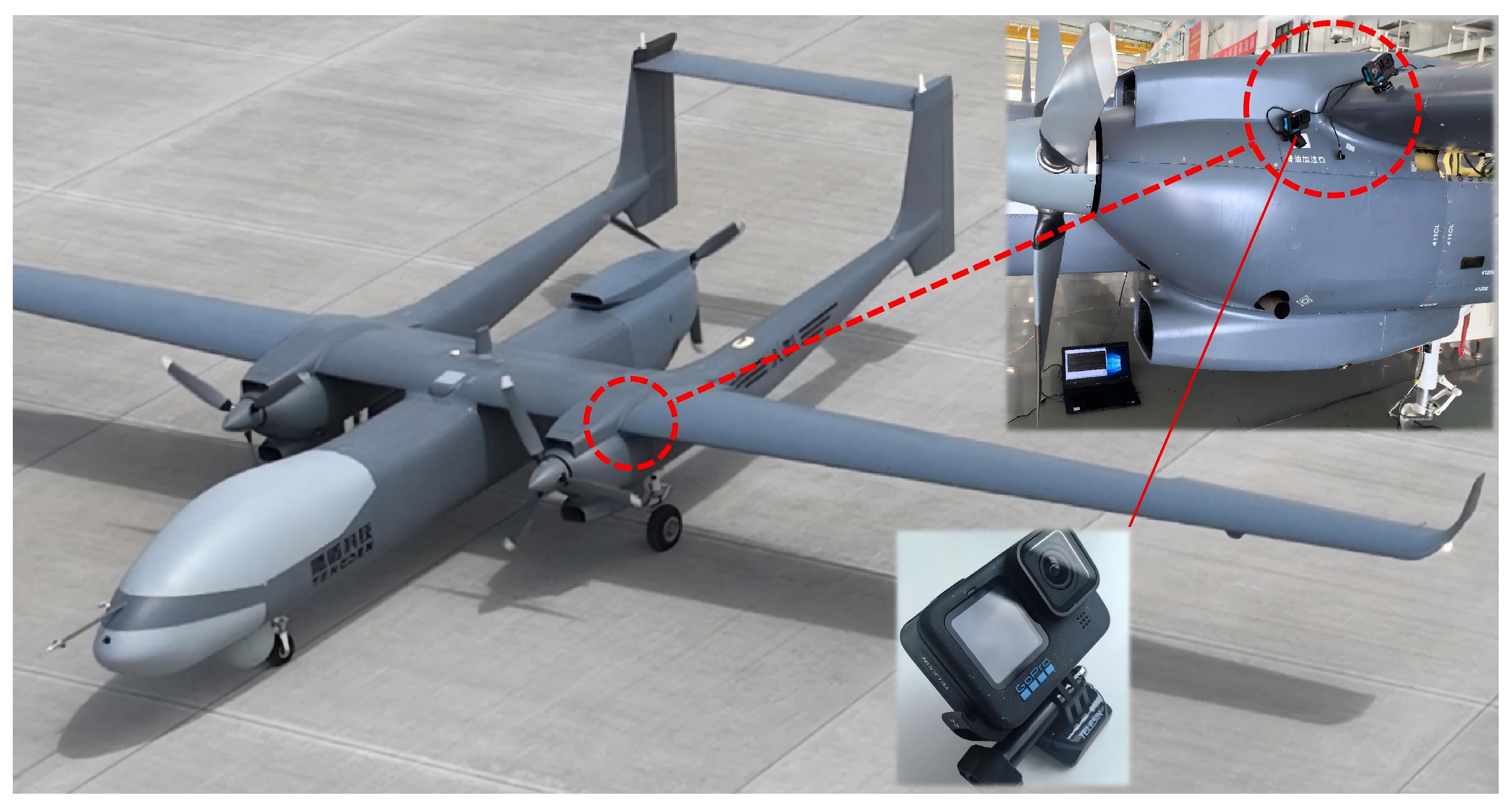
Figure 2.
Examples of real flight wing icing images covering eight typical scenarios ordered by icing extent: (a) early-stage icing, (b) scattered ice crystals, (c) leading-edge icing, (d) upper-surface frost ice, (e) low-contrast glaze ice, (f) cloud background, (g) strong glare, (h) blurred boundary. Red contours indicate ground-truth boundaries.
Figure 2.
Examples of real flight wing icing images covering eight typical scenarios ordered by icing extent: (a) early-stage icing, (b) scattered ice crystals, (c) leading-edge icing, (d) upper-surface frost ice, (e) low-contrast glaze ice, (f) cloud background, (g) strong glare, (h) blurred boundary. Red contours indicate ground-truth boundaries.
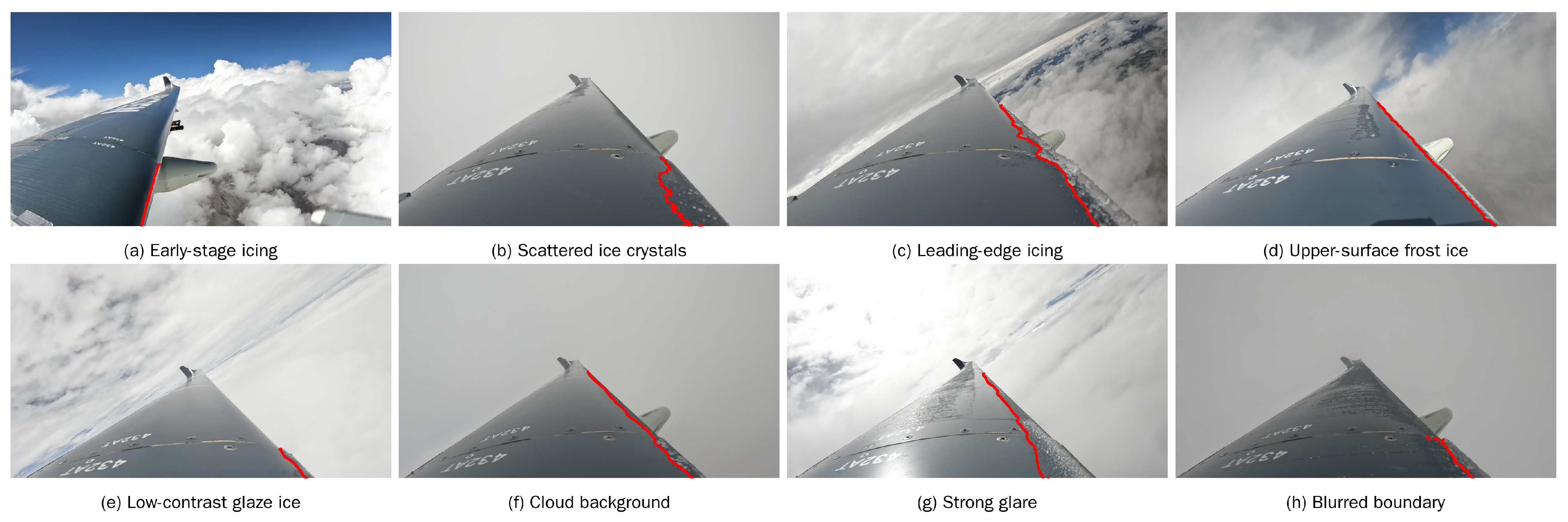
Figure 3.
Baseline model comparison on the flight-wise test set. (a) PA, Precision, Recall, IoU, Dice; (b) number of parameters.
Figure 3.
Baseline model comparison on the flight-wise test set. (a) PA, Precision, Recall, IoU, Dice; (b) number of parameters.
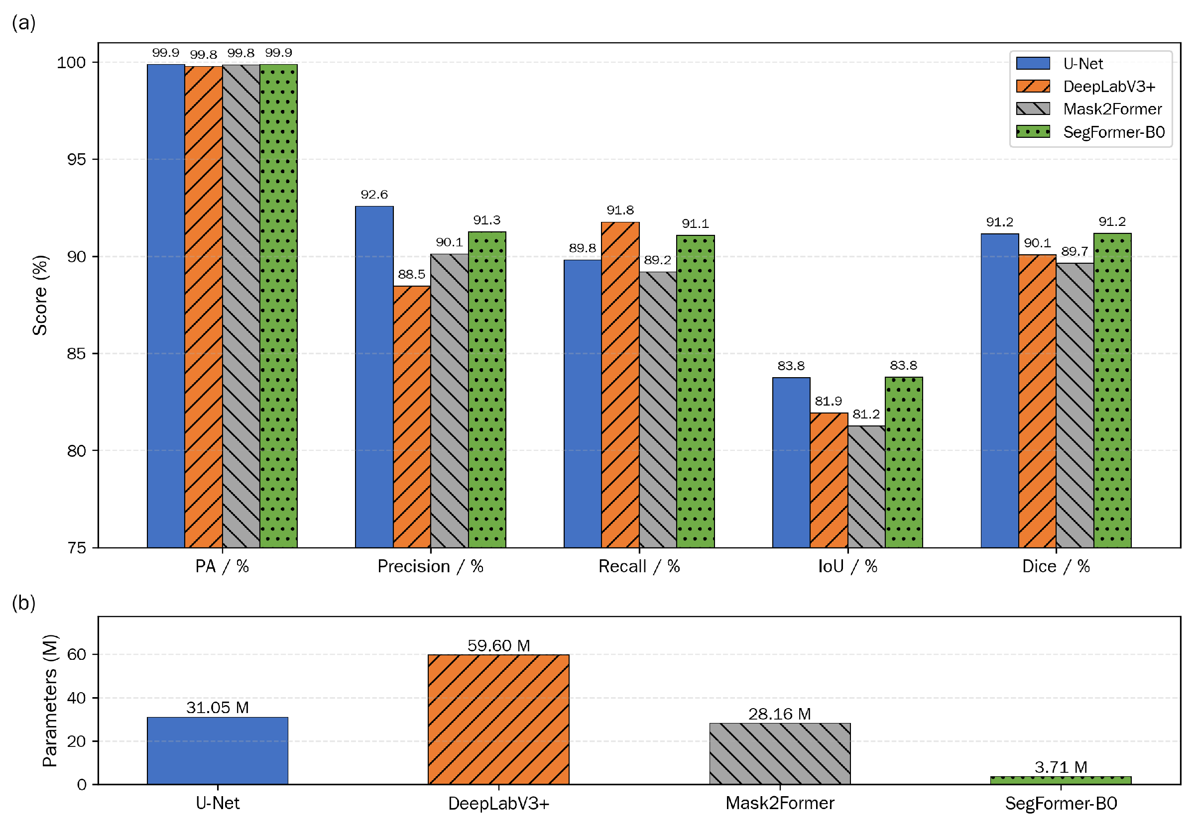
Figure 4.
Attention ablation results: Exp-5 (SENet+CBAM) achieved the highest Dice (91.65%) and IoU (84.58%) among the attention variants. Exp-8 (three-attention stacking) had the highest Recall but the lowest Precision. See Table 12 for detailed values.
Figure 4.
Attention ablation results: Exp-5 (SENet+CBAM) achieved the highest Dice (91.65%) and IoU (84.58%) among the attention variants. Exp-8 (three-attention stacking) had the highest Recall but the lowest Precision. See Table 12 for detailed values.
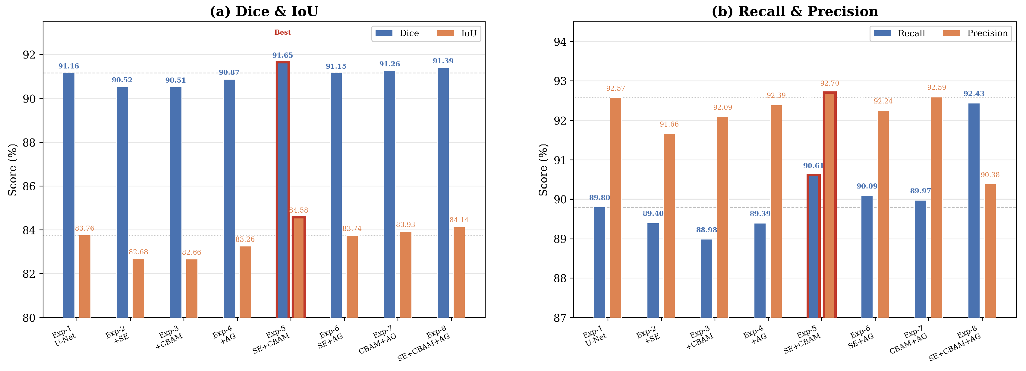
Figure 5.
Segmentation results on challenging scenarios: (a) early-stage weak icing, (b) scattered small ice crystals, (c) low-contrast thin ice, (d) cloud background, (e) blurred boundary. In error maps: red = false positive, blue = false negative, gray = correct.
Figure 5.
Segmentation results on challenging scenarios: (a) early-stage weak icing, (b) scattered small ice crystals, (c) low-contrast thin ice, (d) cloud background, (e) blurred boundary. In error maps: red = false positive, blue = false negative, gray = correct.
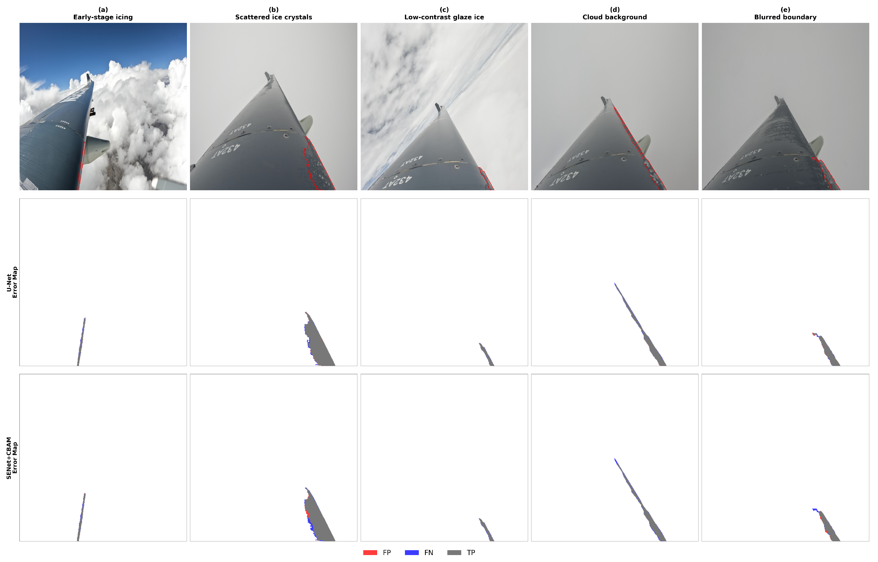
Figure 6.
Ice boundary local-zoom comparison: U-Net, SENet+CBAM, and +ROI boundary loss predictions (colored contours) vs. ground truth (green contours), on three small-area icing samples (–). +ROI boundary loss shows improved boundary overlap, consistent with the Recall gain reported in Table 13.
Figure 6.
Ice boundary local-zoom comparison: U-Net, SENet+CBAM, and +ROI boundary loss predictions (colored contours) vs. ground truth (green contours), on three small-area icing samples (–). +ROI boundary loss shows improved boundary overlap, consistent with the Recall gain reported in Table 13.
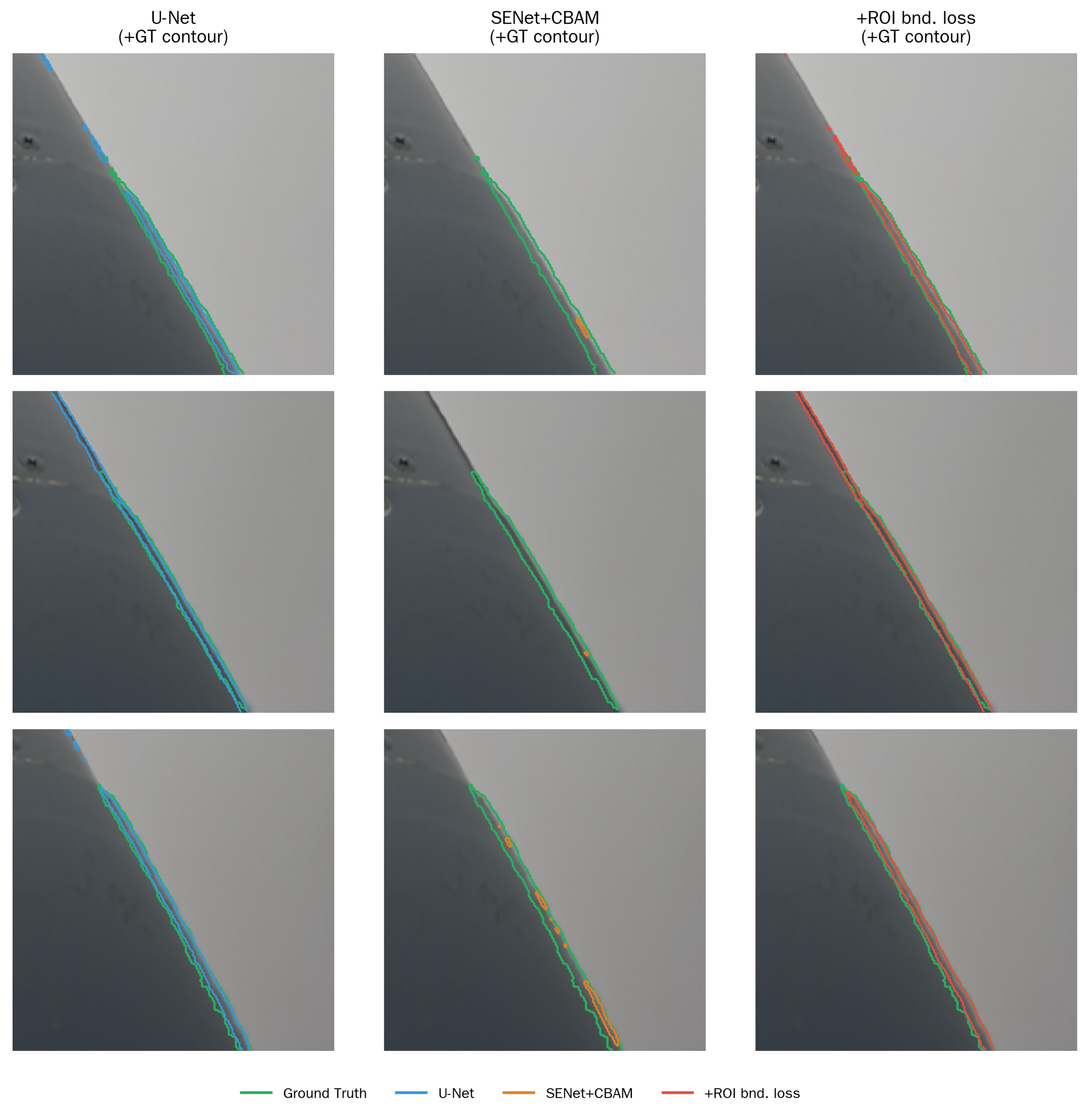
Figure 7.
Frame-to-frame Dice fluctuation curves. Red curve: original prediction; blue curve: after inter-frame smoothing. Each subplot corresponds to one test sortie.
Figure 7.
Frame-to-frame Dice fluctuation curves. Red curve: original prediction; blue curve: after inter-frame smoothing. Each subplot corresponds to one test sortie.
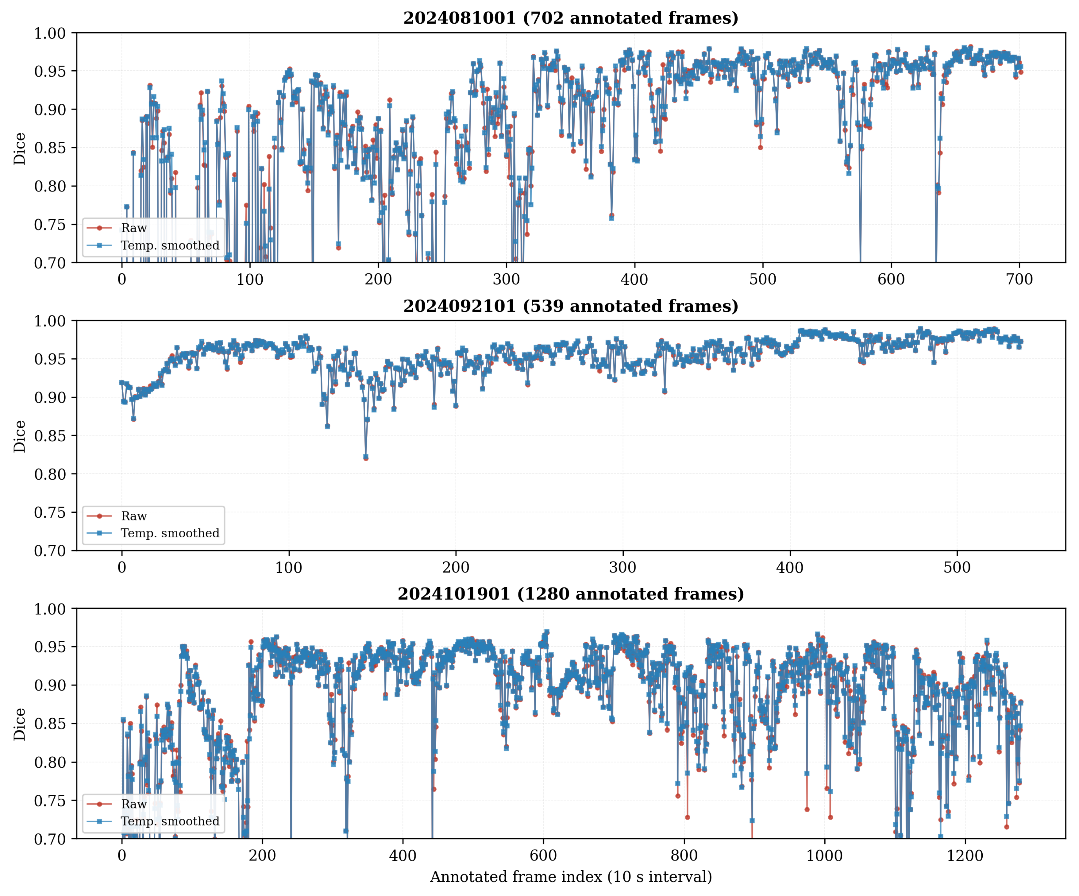
Figure 8.
Ice-area ratio time series for the three test sorties. Blue thin line: Exp-11 prediction on 2 s dense frames; dark-gray triangles: GT at annotated frames; colored circles: predicted values at annotated frames. Error statistics and sortie details in Table 17.
Figure 8.
Ice-area ratio time series for the three test sorties. Blue thin line: Exp-11 prediction on 2 s dense frames; dark-gray triangles: GT at annotated frames; colored circles: predicted values at annotated frames. Error statistics and sortie details in Table 17.
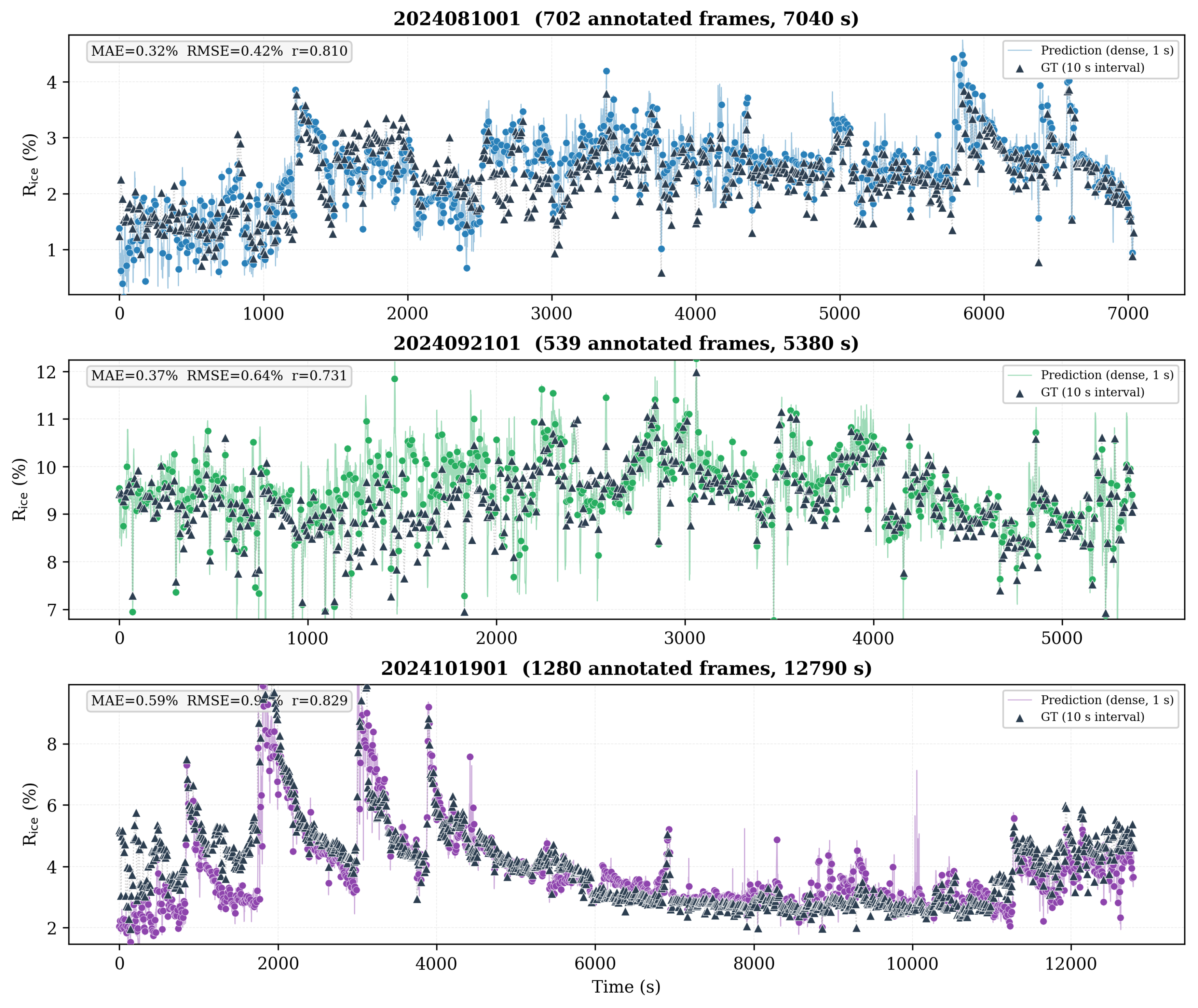
Figure 9.
Typical failure cases. Top: specular-reflection false positives; middle: transparent thin-ice missed detection; bottom: cloud-background false positives. In error maps, red = false positive, blue = false negative, gray = correct. These failures reflect intrinsic limitations of monocular RGB sensing under low-contrast conditions.
Figure 9.
Typical failure cases. Top: specular-reflection false positives; middle: transparent thin-ice missed detection; bottom: cloud-background false positives. In error maps, red = false positive, blue = false negative, gray = correct. These failures reflect intrinsic limitations of monocular RGB sensing under low-contrast conditions.
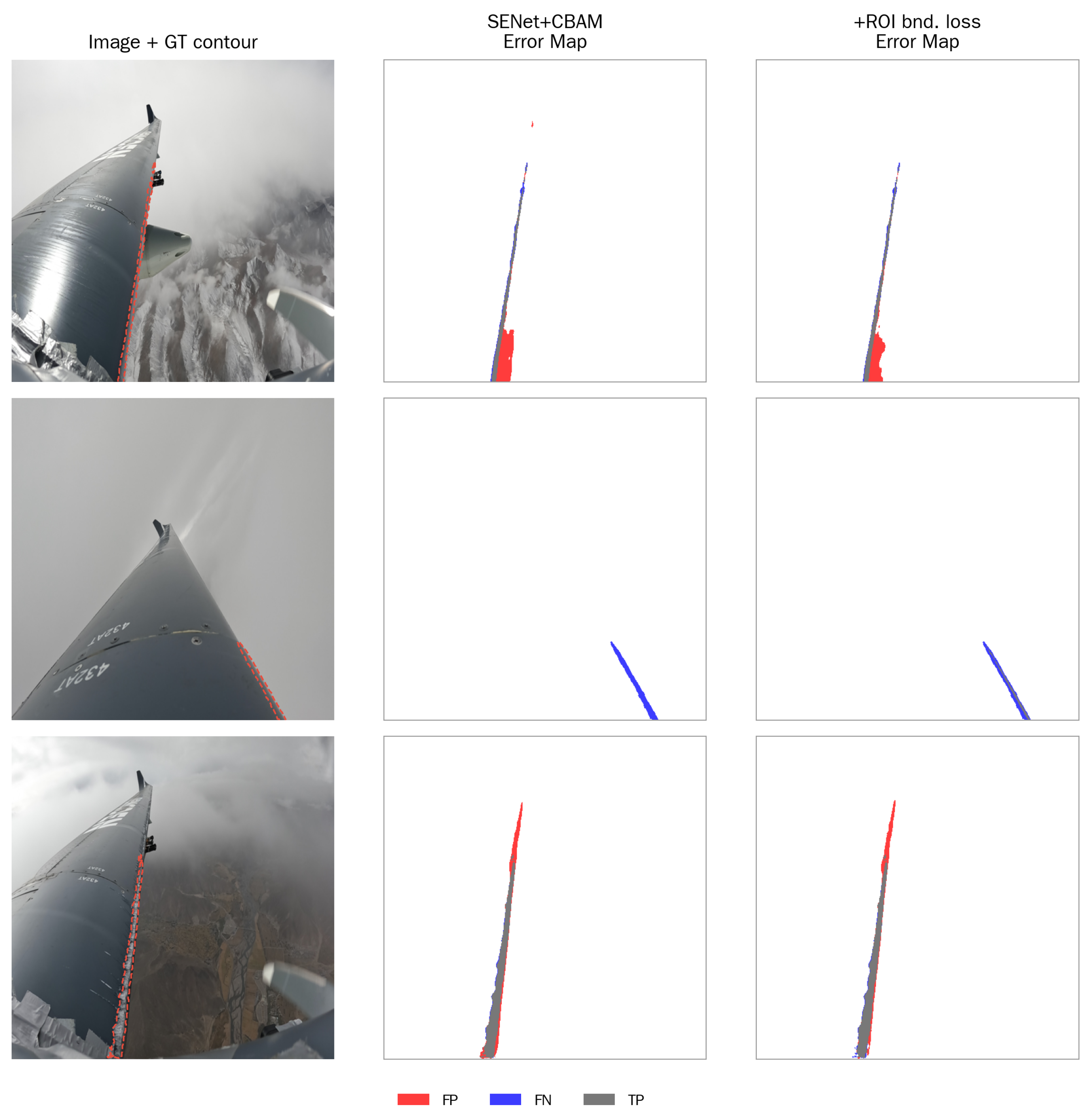
Table 1.
UAV platform and image acquisition parameters.
| Item | Parameter |
|---|---|
| Flight platform | Tengdun Twin-Tailed Scorpion A UAV |
| Camera | GoPro HERO11 Black |
| Mounting position | Near engine nacelle, backward view toward wing surface |
| Image resolution | 1920 × 1080 pixels |
| Frame rate | 24 Hz |
| Stabilization | Enabled |
| Exposure | Automatic |
Table 2.
Flight-test conditions.
| Item | Value |
|---|---|
| Data collection period | July–November 2024 |
| Flight region | Qinghai–Tibet Plateau |
| Number of sorties | 35 |
| Total raw video duration | 106 h |
| Icing or potential icing duration | ∼39 h |
Table 3.
Annotation quality control statistics.
| Item | Value |
|---|---|
| Total annotated images | 13,894 |
| Manual key-frame ratio | ∼10% |
| Annotation tool | ISAT-SAM / SAM2 |
| Annotation format | Binary mask |
Table 4.
Dataset minimal metadata fields.
| Field | Description |
|---|---|
| image_path | Image file path |
| mask_path | Mask file path |
| sortie_id | Flight date or sortie number |
| split | train / val / test |
Table 5.
Model training configuration.
| Item | U-Net / DeepLabV3+ / SegFormer-B0 | Mask2Former |
|---|---|---|
| Input size | 512 × 512 | 512 × 512 (multi-scale training) |
| Batch size | 6 | 4 |
| Epochs / Iterations | 30 epochs | 82,020 iterations |
| Initial learning rate | ||
| Optimizer | AdamW | AdamW |
| LR scheduler | ReduceLROnPlateau | WarmupPolyLR |
| Patience | 5 | – |
| Primary loss | BCEWithLogitsLoss | CrossEntropy |
| Auxiliary loss | Dice Loss | Dice Loss + Mask Loss |
| Loss weight | 1:1 | – |
| Framework | PyTorch 2.4.0 + transformers | detectron2 / PyTorch 2.8.0 |
| CUDA | 12.6 | 12.8 |
Table 6.
Attention mechanism ablation experiment design.
| Exp. | Configuration | Attention | Purpose |
|---|---|---|---|
| Exp-1 | Baseline | None | U-Net baseline |
| Exp-2 | SENet | SENet | Channel attention |
| Exp-3 | CBAM | CBAM | Channel–spatial attention |
| Exp-4 | Attention U-Net | Attention Gate | Skip-connection gating |
| Exp-5 | SENet + CBAM | SENet + CBAM | Channel & spatial combination |
| Exp-6 | SENet + Attn U-Net | SENet + Attn Gate | Channel attention + gating |
| Exp-7 | CBAM + Attn U-Net | CBAM + Attn Gate | Spatial attention + gating |
| Exp-8 | All attention | SENet + CBAM + Attn Gate | Multi-attention stacking |
Table 7.
Extended ablation experiment design.
| Exp. | Configuration | Attention | ROI Mask | Bnd. Weight | Temp. Smooth. |
|---|---|---|---|---|---|
| Exp-5 | SENet+CBAM | Yes | – | – | – |
| Exp-9a | + ROI-only loss | Yes | Yes | – | – |
| Exp-9b | + boundary-only loss | Yes | – | Yes | – |
| Exp-9 | + ROI + boundary loss | Yes | Yes | Yes | – |
| Exp-10 | + temporal smoothing | Yes | – | – | Yes |
| Exp-11 | + ROI + bnd. loss + temp. smooth. | Yes | Yes | Yes | Yes |
Table 8.
Onboard deployment platform configuration.
| Component | Specification |
|---|---|
| Platform | MIC-770V3 industrial computer |
| CPU | Intel Core i5-12500 (6C/12T, 3.0 GHz, Alder Lake) |
| GPU | NVIDIA RTX A2000 Embedded 8 GB (SKY-MXM-A2000-8SDA, MXM) |
| GPU cores | GA106, 2,560 CUDA cores |
| Operating system | Windows |
| Python | 3.12 |
| Deep learning framework | PyTorch 2.7.1+cu128 |
| CUDA | 12.8 |
| OpenCV | 4.13.0 |
Table 9.
Dataset split statistics. For the flight-wise split, each cell reports sorties/images.
| Split Method | Training | Validation | Test |
|---|---|---|---|
| Flight-wise (primary) | 16 / 9,719 | 3 / 1,651 | 3 / 2,524 |
| Image-level random (ref.) | 10,934 | 1,562 | 1,398 |
Table 10.
Monthly distribution of the flight-wise split (number of sorties).
| Month | Train | Val | Test |
|---|---|---|---|
| Jul. 2024 | 1 | 0 | 0 |
| Aug. 2024 | 7 | 1 | 1 |
| Sep. 2024 | 7 | 2 | 1 |
| Oct. 2024 | 1 | 0 | 1 |
| Total | 16 | 3 | 3 |
Table 12.
Attention mechanism ablation results (flight-wise test set).
| Exp. | Model | PA/% | Precision/% | Recall/% | IoU/% | Dice/% | Params/M |
|---|---|---|---|---|---|---|---|
| Exp-1 | U-Net baseline | 99.88 | 92.57 | 89.80 | 83.76 | 91.16 | 31.05 |
| Exp-2 | U-Net + SENet | 99.87 | 91.66 | 89.40 | 82.68 | 90.52 | 31.09 |
| Exp-3 | U-Net + CBAM | 99.87 | 92.09 | 88.98 | 82.66 | 90.51 | 31.09 |
| Exp-4 | Attention U-Net | 99.87 | 92.39 | 89.39 | 83.26 | 90.87 | 31.75 |
| Exp-5 | SENet + CBAM | 99.88 | 92.70 | 90.61 | 84.58 | 91.65 | 31.14 |
| Exp-6 | SENet + Attention U-Net | 99.88 | 92.24 | 90.09 | 83.74 | 91.15 | 31.79 |
| Exp-7 | CBAM + Attention U-Net | 99.88 | 92.59 | 89.97 | 83.93 | 91.26 | 31.79 |
| Exp-8 | SE + CBAM + Attention U-Net | 99.88 | 90.38 | 92.43 | 84.14 | 91.39 | 31.83 |
Table 13.
Segmentation performance across ice-area ratio groups (flight-wise test set, ROI-constrained statistics, five-model comparison).
Table 13.
Segmentation performance across ice-area ratio groups (flight-wise test set, ROI-constrained statistics, five-model comparison).
| Images | Dice/% | Recall/% | |||||||||
|---|---|---|---|---|---|---|---|---|---|---|---|
| U-Net | SE+CBAM | +ROI | +Bnd. | +ROI+B | U-Net | SE+CBAM | +ROI | +Bnd. | +ROI+B | ||
| 1,049 | 88.60 | 85.78 | 87.71 | 88.09 | 88.95 | 91.37 | 86.63 | 90.75 | 93.79 | 92.66 | |
| 841 | 87.27 | 88.23 | 89.09 | 89.41 | 87.95 | 81.85 | 84.21 | 86.32 | 86.36 | 84.37 | |
| 250 | 92.61 | 94.06 | 93.68 | 93.52 | 93.91 | 92.92 | 96.04 | 94.93 | 94.33 | 95.28 | |
| 381 | 94.51 | 94.89 | 93.72 | 93.80 | 94.71 | 94.55 | 95.65 | 94.10 | 95.01 | 94.66 | |
Table 14.
ROI and boundary-weighted loss decomposition and inter-frame smoothing extended ablation results (flight-wise test set).
Table 14.
ROI and boundary-weighted loss decomposition and inter-frame smoothing extended ablation results (flight-wise test set).
| Exp. | Model | PA/% | Prec./% | Recall/% | IoU/% | Dice/% | |
|---|---|---|---|---|---|---|---|
| Exp-5 | SENet + CBAM | 99.88 | 92.70 | 90.61 | 84.58 | 91.65 | |
| Exp-9a | + ROI-only loss | 99.88 | 91.70 | 91.47 | 84.48 | 91.59 | |
| Exp-9b | + Boundary-only loss | 99.88 | 91.16 | 92.08 | 84.53 | 91.62 | |
| Exp-9 | + ROI + boundary loss | 99.88 | 92.03 | 91.32 | 84.63 | 91.68 | |
| Exp-10 | + temporal smoothing | 99.88 | 92.85 | 90.51 | 84.61 | 91.66 | |
| Exp-11 | + ROI boundary loss + temp. smooth. | 99.88 | 92.21 | 91.21 | 84.69 | 91.71 | 3.18 × 10⁻³ |
Table 15.
Inter-frame smoothing ablation results (2 s interval dense-frame evaluation).
| Exp. | Base Model | Annot. Frames | Dice (bef.)/% | Dice (aft.)/% | (bef.) | (aft.) | |
|---|---|---|---|---|---|---|---|
| Exp-10 | Exp-5 | 2,518 | 91.65 | 91.66 | 0.5% | ||
| Exp-11 | Exp-9 | 2,518 | 91.68 | 91.71 | 3.18 × 10⁻³ | 3.3% |
Table 16.
Per-sortie analysis (Exp-11).
| Test Sortie | Annot. Frames | (bef.) | (aft.) | |
|---|---|---|---|---|
| 2024081001 | 702 | |||
| 2024092101 | 536 | |||
| 2024101901 | 1,280 |
Table 17.
Ice-area ratio time-series error statistics (Exp-11).
| Icing Event | Duration/s | Frames | MAE/% | RMSE/% | Correlation |
|---|---|---|---|---|---|
| Event 1 (2024081001) | 7,040 | 702 | 0.319 | 0.421 | 0.8099 |
| Event 2 (2024092101) | 5,380 | 536 | 0.369 | 0.643 | 0.7315 |
| Event 3 (2024101901) | 12,790 | 1,280 | 0.594 | 0.912 | 0.8287 |
Table 20.
Per-frame processing latency on the MIC-770V3 onboard embedded platform (, 10 min icing video test frames).
Table 20.
Per-frame processing latency on the MIC-770V3 onboard embedded platform (, 10 min icing video test frames).
| Stage | Mean/ms |
|---|---|
| Image preprocessing | 16.34 |
| GPU inference | 71.44 |
| Optical-flow post-process. (CPU) | 40.45 |
| Post-processing (warp + EMA + occlusion) | 6.36 |
| Total processing time | 134.59 |
Table 21.
Onboard deployment system resource usage (measured over the 600 s continuous-operation test, sampled at the 2 s detection interval).
Table 21.
Onboard deployment system resource usage (measured over the 600 s continuous-operation test, sampled at the 2 s detection interval).
| Metric | Mean | Note |
|---|---|---|
| CPU utilization | 17.1% | Including OS background load |
| Memory usage | 20,694 MB | – |
| GPU memory usage | 1,204 MB | ∼14.7% of 8 GB total |
| GPU utilization | 16.7% | 2 s/frame intermittent inference |
| GPU temperature | 44.2 °C | Passive embedded cooling |
| GPU power | 20.7 W | Intermittent inference average |
Table 22.
Continuous operation stability test results.
| Metric | Value |
|---|---|
| Continuous run time | 600 s |
| Detection interval | 2 s/frame |
| Theoretical inference count | ≈301 |
| Actual valid inference count | 301 |
| Program crashes | 0 |
| Inference interruptions | 0 |
Disclaimer/Publisher’s Note: The statements, opinions and data contained in all publications are solely those of the individual author(s) and contributor(s) and not of MDPI and/or the editor(s). MDPI and/or the editor(s) disclaim responsibility for any injury to people or property resulting from any ideas, methods, instructions or products referred to in the content. |
© 2026 by the authors. Licensee MDPI, Basel, Switzerland. This article is an open access article distributed under the terms and conditions of the Creative Commons Attribution (CC BY) license (http://creativecommons.org/licenses/by/4.0/).
Copyright: This open access article is published under a Creative Commons CC BY 4.0 license, which permit the free download, distribution, and reuse, provided that the author and preprint are cited in any reuse.