
Submitted:
26 August 2026
Posted:
27 August 2026
You are already at the latest version
Abstract
Propellant feed systems for small liquid rocket engines are commonly modelled as hydraulic networks discharging into a prescribed chamber pressure. Such models cannot represent the feedback between delivered mass flow and chamber pressure, and therefore cannot predict injector stiffness, startup coupling, or feed-coupled instability—the quantities the model is usually built to inform. We replace the prescribed boundary condition in a Simscape Fluids model of a gaseous-oxygen/kerosene feed system with a lumped-volume combustion chamber whose pressure is a state, closed through a choked throat and thermochemistry interpolated on instantaneous mixture ratio. The coupled model reproduces the analytical steady state pc=m˙c*/At to better than 10−3%, and predicts an operating point far from the design point that the open-loop model reports as nominal. A linear analysis of the coupled system yields a closed-form low-frequency stability boundary, Δpinj/pc< [2(1+O/F)]-1, recovering the classical twenty-percent injector-stiffness rule from first principles. A mechanism-separation procedure distinguishes feed-coupled chug from a mixture-ratio/c* instability that requires no feed inertia at all.
Keywords:
liquid rocket engine
; propellant feed system
; Simscape Fluids
; combustion chamber coupling
; injector stiffness
; chug instability
; lumped-parameter modelling
; gaseous oxygen
; kerosene
1. Introduction
Small bipropellant rocket engines built by university and amateur teams are almost always designed with a two-stage toolchain: an equilibrium thermochemistry code fixes the chamber conditions and nozzle geometry at a chosen mixture ratio, and a separate hydraulic network model sizes the plumbing that must deliver those propellant flows [1,2]. The two stages are usually coupled only in one direction. The thermochemistry code supplies a design chamber pressure, and the feed model treats that pressure as a fixed downstream boundary condition.
System-level, one-dimensional models of this kind are the established engineering tool for propulsion analysis. Dedicated environments exist for the purpose: ESPSS/EcosimPro is the European standard for space propulsion system simulation [3], and recent reviews survey the transient modelling approaches in use across the field [4]. General-purpose multi-domain libraries such as Simscape Fluids [5] are increasingly applied to the same task, while method-of-characteristics solvers are used where the propellant lines must be resolved as distributed systems [6], and component-level models validated against test data have been reported for the LOX/methane class [7]. Outside propulsion the same philosophy—low-order components assembled into a network and validated against transient measurements—is long established in hydraulic power systems [8], in pipeline transients [9], and in two-phase thermal devices [10].
This is a reasonable engineering simplification at the design point, and it is the standard architecture of the Simscape Fluids feed-system models that have become common in this community. It has a structural consequence that is less widely appreciated: a feed model with a prescribed chamber pressure cannot predict what happens when the feed system fails to deliver the design flow. The chamber pressure it reports is an input, not a result. Injector stiffness computed from it is the stiffness the designer assumed, not the stiffness the hardware will have. Startup transients are whatever ramp was scripted. And low-frequency feed-coupled instability—chug—is by construction impossible, because chug is precisely a feedback loop through the chamber [11,12,13,14].
Low-frequency instability has been treated with combustion time-lag models since Summerfield’s original analysis [11], and double-time-lag formulations remain in use for predicting chugging during start-up in system-level codes [15]. It remains a live concern wherever the injector pressure drop is small relative to chamber pressure, as in deep-throttled engines [16] and in small thrusters operated by pulse-width modulation [17]; analogous low-frequency modes arise in hybrid motors [18] and in cryogenic feed lines [19]. What these analyses have in common is that the chamber pressure is a state of the model, which is precisely what the open-loop feed model gives up.
The distinction matters most when the hardware does not match the design, which for a first-iteration engine is the normal case rather than the exception. The system studied here supplies two concrete instances. Its oxidiser flow turns out to be set by a quarter-inch gate valve that is choked at the operating point, so the oxidiser injector—the component sized to meter that flow—has almost no authority over it. And a cold-flow calibration of the fuel injector, reported in Section 3.2, shows the effective discharge area carried by the model to be 19 to 40 larger than the bench value. Neither discrepancy is visible in a model that holds chamber pressure fixed: the first because the consequence of the restriction is absorbed by the imposed boundary, and the second because the resulting flow error is never propagated into a pressure the rest of the system can respond to.
In this work we take an existing, working Simscape Fluids model of a gaseous-oxygen (GOX)/kerosene feed system for a nominally 100 N engine and replace its prescribed-pressure chamber with a lumped-volume chamber whose pressure is an integrated state. The contribution is threefold. First, we give the coupled formulation and its verification, together with a reproducible build procedure that derives the coupled model from the open-loop one by script rather than by hand. Second, we show what the coupling changes: the predicted operating point moves substantially, and the mechanism by which it moves is a feedback path the open-loop model cannot express. Third, we derive a closed-form low-frequency stability boundary for the coupled system and use it, together with a numerical mechanism-separation procedure, to distinguish genuine feed-coupled chug from a mixture-ratio instability that involves the feed line only incidentally.
2. Materials and Methods
2.1. Engine and Feed System
The engine is a pressure-fed GOX/kerosene thrust chamber designed for at . Chamber geometry follows from an equilibrium analysis at : throat diameter (), characteristic length (chamber volume ), and nozzle area ratio . The design mass flows are and .
Figure 1 shows the feed system. It is drawn from the active blocks of the executed model: several components present in the Simulink diagram—a poppet main oxidiser valve, a ball valve, a relief valve and several line segments—are commented out in the model as delivered and are therefore absent here, so that the schematic and the simulated system agree.
The oxidizer circuit runs from a 10 bottle at 150 through a dome-loaded regulator set to , approximately 1 of line, a quarter-inch gate valve acting as the main oxidiser valve, a further metre of line, and the oxidiser injector orifice. The fuel circuit is a positive-displacement pump represented as a constant pressure rise of , a short 20 line, a solenoid main fuel valve, and the fuel injector orifice. Full component parameters are given in Appendix A.
2.2. Baseline Open-Loop Model
The baseline model is implemented in Simscape Fluids [5] (MATLAB R2023b) using the isothermal-liquid domain for kerosene and the gas domain for oxygen. The combustion chamber is represented by two controlled reservoirs, one in each domain, both driven by a prescribed pressure
with . Thrust is reported as with a fixed .
2.3. Coupled Chamber Formulation
We replace Equation (1) with a mass balance on a constant-volume chamber holding a perfect gas at the equilibrium flame temperature and discharging through the throat. With and ,
The throat mass flow uses the choked and subsonic branches of the isentropic nozzle relation, with and :
At steady state Equation (2) recovers the textbook result , which we use as the primary verification case in Section 3.1. The associated filling time constant is
which evaluates to at the design condition—two orders of magnitude faster than the 200 asserted by Equation (1).
Thrust is obtained from the vacuum thrust coefficient with an explicit ambient correction,
which at the design point returns against the optimum-expansion value from the design code.
2.3.1. Ignition and Extinction
A step change of the chamber boundary from ambient to flame temperature is both unphysical and numerically intractable: it causes the transient initialisation of the Simscape gas network to fail to converge. We therefore introduce a combustion progress variable ,
with flame-establishment constant . Chamber properties are blended between unreacted oxygen and equilibrium combustion by ; the smooth gate g makes ignition conditional on both propellants being present, so loss of either extinguishes the chamber and shutdown is a physical blowdown rather than a scripted ramp. Before ignition only the gaseous oxidiser pressurises the chamber, the liquid fuel being blended into the gas-phase source term by .
2.3.2. Thermochemistry
, , and are interpolated on the instantaneous mixture ratio from an equilibrium table. The gas constant is taken from the tabulated triple as , so that throat flow and chamber filling remain mutually consistent with the tabulated rather than being independently parameterised.
The table is generated with NASA CEA [20] for RP-1/ at , finite-area combustor with , equilibrium composition, at 19 mixture ratios from to . The spacing is deliberately dense below because, as Section 3.3 shows, the as-built feed system drives the engine into that region, and it is the local slope there that governs the behaviour examined in Section 3.5. All 19 cases converged.
Two consistency checks are applied to the parsed table. The molar mass implied by is compared with the molar mass CEA reports directly, and agrees to within across the full range, which confirms that the chamber station has been identified correctly in every block; the finite-area listing prints both an injector and a combustion-end station, and these differ by only in temperature, so a misidentification would otherwise be silent. Separately, the row reproduces the project’s pre-existing independent CEA run to all printed digits (, , , ).
2.4. Feed-Line Dynamics
Fluid inertia is enabled in the liquid line, giving the momentum state with inertance . For the fuel line, and , giving . The Simscape gas pipe has no inertance term; this asymmetry is acceptable here because the oxidiser line is choked at the gate valve, which acoustically isolates everything upstream of it from the chamber, and because gas inertance is smaller by orders of magnitude.
This lumped inertance–resistance–capacitance representation is the low-order limit of the distributed water-hammer equations that govern liquid line transients [9,21]. It deliberately does not resolve the unsteady wall friction and geometry corrections that become significant when a line is modelled in detail [22,23], nor the column separation and cavitation that accompany severe transients [24]. The justification is one of scale. With the modelled kerosene properties (, ) the acoustic speed is 1650 /, so the first quarter-wave mode of the fuel line lies near 390 —a factor of three above the 130 phenomena examined in Section 3.5. The lumped inertance therefore places the low-frequency response correctly even though it cannot represent the wave behaviour above it.
The oxidiser main valve is represented by a flow-coefficient () model with a critical pressure ratio, which is the standard treatment for a gas restriction driven into choking; experimental characterisation of choked discharge through a gas restrictor [25] and of the onset of choking in calibrated liquid orifices [26] supports the use of a single coefficient with a switched critical branch, and it is this element that Section 3.3 identifies as controlling the whole engine.
With the momentum state present, the line initial pressure must be consistent with its source: the fuel line is therefore initialised at the pump outlet pressure of rather than at ambient. An inconsistent initialisation is harmless in a purely resistive–capacitive line, which relaxes it in a single solver step, but in a dead-ended line with inertia it excites a lightly damped resonance that persists for the whole run, since without through-flow there is almost no dissipation to remove it.
2.5. Cold-Flow Bench Data
The fuel injector was characterised on a cold-flow bench before the model was built. The element is a swirl injector (Mejarra INJ 001) with a documented fuel orifice diameter of , giving a geometric area of . The working fluid on the bench was water, not kerosene.
Flow was measured with an inline turbine flowmeter and pressure at four taps, logged asynchronously at approximately 1 each. Two taps (, ) follow the water flow closely (correlation with flow rate and over the flowing portion of the record); the remaining two are on a separate circuit that is pressurised only in the second half of the run and are excluded from the analysis.
Because the bench fluid differs from the propellant, the quantity transferred to the model is the effective discharge area rather than or A separately. From
is independent of which incompressible fluid was used, whereas and A are not separately identifiable from flow data alone. This is not merely a bookkeeping convenience: the discharge coefficient of a small orifice is not a constant of the geometry but depends on Reynolds number, on inlet chamfer and edge condition, and on whether the orifice cavitates, effects that have been resolved experimentally for circular and chamfered orifices [27] and for injector passages under fuel-injection conditions [28]. Reporting the lumped product avoids attributing the discrepancy to either factor on evidence that cannot distinguish them. Comparable direct measurement of injector mass flow, rather than inference from an assumed coefficient, is reported for self-pressurising propellants in [29].
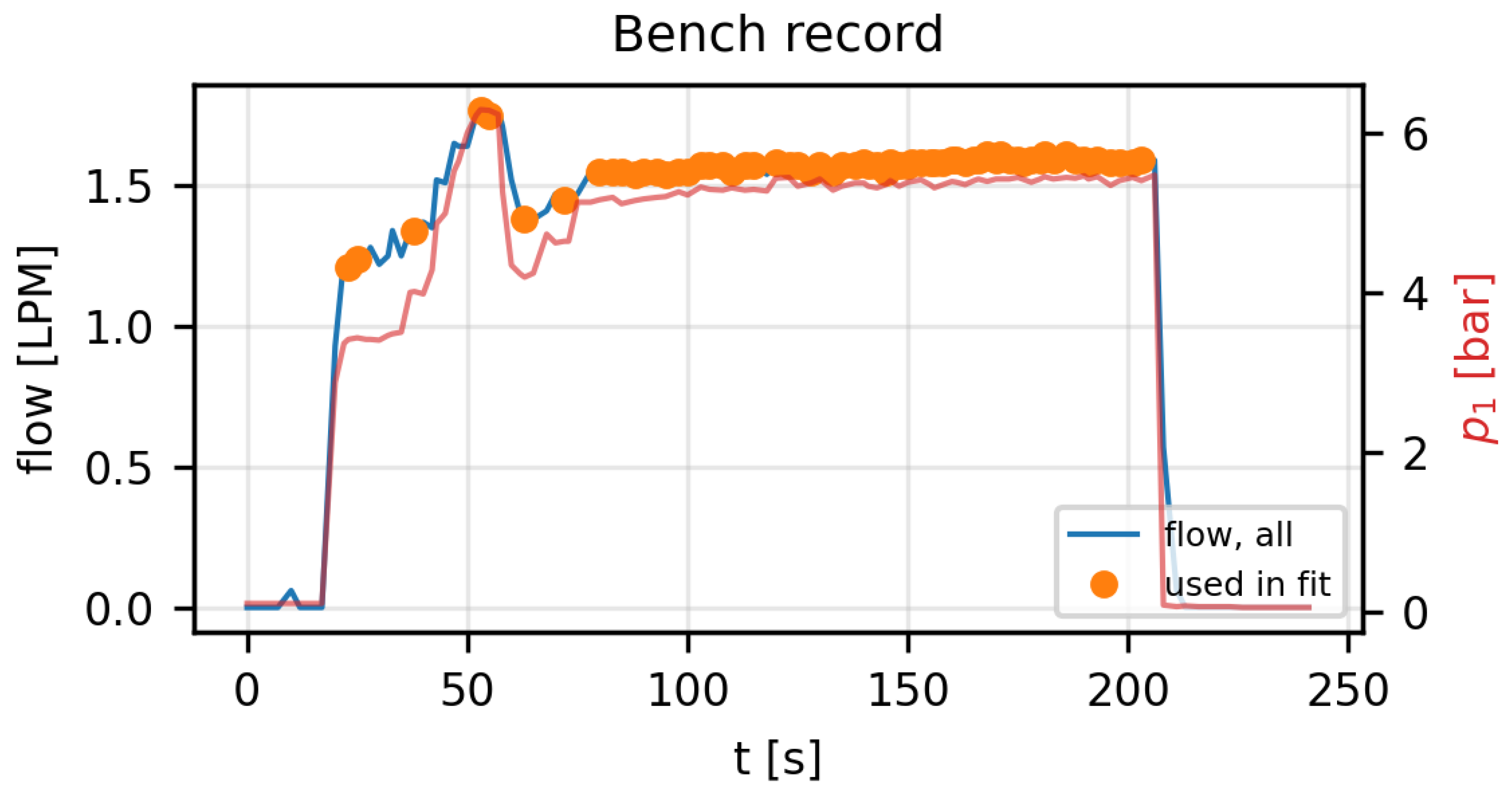
The flowmeter and the transducers are logged on independent cycles, so during the pump ramp a flow sample can be paired with a pressure sample up to 2 stale. We therefore fit only quasi-steady samples, defined as those for which both flow and upstream pressure differ from their immediate neighbours by less than 3 . This retains 66 of 117 aligned samples; Figure 3 shows the record and which samples survived.
2.6. Combustion Time Lag
Propellant crossing the injector face does not release its heat there; it must atomise, vaporise and mix. The chamber therefore burns what was injected earlier, implemented as a pure transport delay on the gas-phase source term. This is the of the Crocco–Cheng n– formulation [11,12]. A pure delay is used rather than a first-order lag because the destabilising mechanism depends on the unbounded phase roll-off of a true delay. We treat as a swept parameter rather than predicting it; constant- and variable-lag closures for the same quantity, and their effect on predicted chug boundaries, are compared in [15].
2.7. Numerical Implementation
The coupled model is generated from the open-loop model by a build script, which replaces the chamber subsystem, writes all parameters into the model workspace, and configures the solver. The model is therefore self-contained and the derivation reproducible. Simulations use ode23t with relative and absolute tolerances of and a maximum step of 1 , chosen so that the filling constant of Equation (4) is resolved.
3. Results
3.1. Verification
The steady operating point of the coupled model reproduces to better than %, evaluated independently from the interpolated at the simulated mixture ratio. The thrust relation, Equation (5), returns at the design point against from the design code, a agreement that confirms the convention and the ambient correction.
3.2. Validation Against Cold-Flow Data
Figure 2 shows the bench data fitted to Equation (7). The discharge law holds well over the range covered: with a mean absolute residual of and all points inside on the parity plot.
Figure 3.
Bench record of the fuel injector run, showing which samples passed the quasi-steady filter (66 of 117). Flow on the left axis, upstream pressure on the right.
Figure 3.
Bench record of the fuel injector run, showing which samples passed the quasi-steady filter (66 of 117). Flow on the left axis, upstream pressure on the right.
The instrumentation does not identify unambiguously which tap pair bounds the injector, so both plausible readings are reported in Table 1. They bracket the answer, and the conclusion is the same either way: the model over-predicts the fuel injector effective discharge area by 19 to 40 .
The model reaches its through a physically implausible pair of values: an area of (equivalent diameter , against a documented ) with a compensating of 0.288. Only the product enters the flow calculation, so this does not by itself invalidate the model, but it means the individual parameters cannot be interpreted physically and the agreement with the bench is worse than the plausible-looking suggests.
Two limitations bound how much this calibration establishes, and both are limitations of the available measurement rather than of the fit. First, the fitted range spans a factor of about 1.9 in , so the square-root law is exercised but not strongly tested; the result is closer to a calibration at one operating point with scatter than to a demonstration of the exponent. Second, the quoted intervals are bootstrap estimates of precision only. The dominant uncertainty is systematic: the turbine flowmeter K-factor was taken from the manufacturer’s nominal value and neither it nor the pressure transducer calibrations were verified against a reference, so no total uncertainty can be quoted. An independent check—a timed gravimetric catch, or a calibration certificate traceable to a standard—would be required before the interval widths in Table 1 could be read as accuracy.
We nonetheless regard the direction of the discrepancy as established, because it is far larger than any plausible instrument error: closing a 19–40 gap in by calibration error alone would require the flowmeter to be in error by a similar proportion, an order of magnitude beyond the specification of a turbine meter in its rated range. The magnitude, by contrast, should be treated as provisional.
The oxidiser circuit is not validated at all. The oxidiser bench run logged pressures but no flow rate, so no effective discharge area can be extracted from it, and the oxidiser injector area in the model remains the as-designed value carried over from the sizing calculation. This matters less than it otherwise would, for the reason developed in Section 3.3: the oxidiser flow is fixed by choking at the gate valve upstream, so the injector area has almost no influence on it, and the predicted oxidiser flow is insensitive to precisely the parameter that is unvalidated. That argument holds only while the valve remains choked. An engine of this design operated at a higher chamber pressure, or with the gate valve replaced, would move the metering authority back to the injector and would require the oxidiser cold-flow measurement before its predictions could be trusted.
3.2.1. Effect on the Coupled Prediction
Substituting the bench-calibrated into the coupled model, holding at its model value and scaling the area, gives Table 2.
Correcting the injector reduces fuel flow by up to 24 and raises the mixture ratio from 0.252 to 0.333, but the engine remains severely oxidiser-starved and far below its design chamber pressure. The headline conclusion is therefore robust to the injector calibration: it is driven by the choked oxidiser valve, not by the fuel-side parameters. The oxidiser flow is unchanged in all three cases, as expected for a circuit whose flow is set by a choked restriction upstream.
3.3. Effect of Coupling on the Predicted Operating Point
Table 3 compares the open-loop and coupled models against the design point.
Both models agree that the engine is oxidiser-starved, but they disagree on the mechanism and the magnitude. In both, the oxidiser flow is set by the quarter-inch gate valve, which is choked: the measured pressure ratio across it is 0.506 against a critical value of 0.528 for . The oxidiser injector, in contrast, drops only of the available 20 . The circuit is valve-limited, not injector-limited, and the injector consequently has almost no authority over the chamber.
The open-loop model stops there. The coupled model additionally captures the consequence: with free to fall, the fuel injector sees a larger pressure difference and delivers more fuel, which drives the mixture ratio further down, which lowers , which lowers again. Figure 4 shows the resulting divergence between the two models.
Two further quantities follow from the coupled formulation and have no open-loop counterpart at all, because both are defined against a chamber pressure the open-loop model does not compute (Figure 5).
3.4. Linear Stability of the Coupled System
Linearising the fuel line and chamber about a steady point, with the oxidiser treated as constant because its supply is choked, gives
whence the characteristic equation
With this reduces to , whose coefficients are all positive: the system without a combustion lag is unconditionally stable, and enabling fluid inertia alone cannot produce chug.
On the imaginary axis , writing , and , Equation (10) separates into and , so that
A positive root—hence a stability boundary at finite —exists whenever . Substituting and gives the compact result
At this evaluates to . The classical design rule that the injector should drop of order twenty percent of chamber pressure [1,2] thus emerges from the lumped model rather than being imposed on it, in the same spirit as the time-lag stability analyses that established it [11,12] and consistent with the pressure-drop margins reported as limiting in throttled engines [16]. Critical lags and frequencies along the boundary are given in Table 4.
3.5. Mechanism Separation
Introducing the combustion lag produced large-amplitude oscillation for at every injector stiffness tested, including 125 —far inside the stable region predicted by Equation (12)—and at a frequency that depended only on and not on the feed line. Both observations are inconsistent with feed-coupled chug.
To identify the mechanism we repeated the sweep with the thermochemistry lookups frozen at their operating-point values, so that , and separately with fluid inertia disabled (Table 5, Figure 8).
Freezing removes the oscillation by five orders of magnitude, to the numerical noise floor. Removing fluid inertia changes it by less than . The instability is therefore driven entirely by the gain and not at all by feed inertia: it is not chug. The loop is a mixture-ratio oscillation—rising chamber pressure reduces fuel flow by back-pressure, raising O/F, raising , raising chamber pressure further—closed by the combustion lag, with the feed line an incidental participant.
Genuine chug is correctly absent, because the engine’s fuel injector is far stiffer than the boundary of Equation (12) requires.
4. Discussion
4.1. A Prescribed Chamber Pressure Is Not a Boundary Condition
The most consequential finding is structural rather than numerical. Prescribing does not merely fix one variable; it severs the only path by which the feed system learns that it is not delivering the design flow. The open-loop model of this engine reports a fuel injector stiffness of , almost exactly the design intent, while the coupled model of the same hardware reports 125 . Neither number is a modelling error: they are answers to different questions. The first is “what stiffness would the injector have if the chamber reached 10 ?”; the second is “what stiffness does it have?”.
This matters because injector stiffness is normally computed precisely to decide whether an engine is at risk of feed-coupled instability, and the open-loop answer is systematically optimistic in exactly the situation where the question is worth asking—when the chamber pressure falls short. A model that assumes the design chamber pressure will report the design stiffness almost regardless of the hardware.
Section 3.5 illustrates a diagnostic that is cheap and underused in lumped multi-physics models. When a coupled model oscillates, the oscillation is usually attributed to whichever loop the modeller was thinking about. Here the natural attribution—feed-coupled chug, since the feed line carries a momentum state and the chamber a pressure state—was wrong, and two observations gave it away before any further computation: the instability persisted at injector stiffnesses far inside the analytically stable region, and its frequency was insensitive to the feed line.
Freezing a constitutive relation at its operating-point value, so that its gain is removed while everything else is untouched, then settles the question directly. It requires no new formulation, and unlike disabling a component it does not perturb the steady state. We suggest it as a routine check whenever a coupled model produces an instability whose mechanism is being inferred rather than demonstrated.
4.2. Sensitivity to the Thermochemistry Table
Because the coupled model drives the engine to a mixture ratio near 0.25, far from the design value, it operates on a part of the curve that a table built around the design point would represent poorly. During development we ran the model against an interpolated table anchored on the single design-point equilibrium result available at the time, before replacing it with the full nineteen-point sweep of Section 3.3. The comparison is instructive, because it separates which conclusions are robust to the thermochemistry and which are not.
The interpolated table was in error by up to 24 in and by nearly a factor of two in at the fuel-rich end, and—more importantly—gave a local slope at the operating point about 65 larger than the computed one. Since Section 3.5 identifies that slope as the gain closing the oscillation loop, this was the one quantity most likely to overturn a conclusion.
It did not. Replacing the table moved the operating point modestly—chamber pressure from 4.96 to , thrust from 41.1 to , mixture ratio from 0.245 to 0.252—and moved the oscillation amplitude at from to , consistent with the reduced gain. The onset lag, the frequencies, and every qualitative conclusion were unchanged: the engine remains severely oxidiser-starved at roughly half its design chamber pressure, and the oscillation remains a mixture-ratio instability that survives removal of feed inertia and vanishes when the thermochemistry is frozen.
The lesson we would draw is not that the table did not matter, but that its influence was confined to the quantities one would expect it to set. A reader adapting this approach should establish the same separation explicitly rather than assume it, particularly if their operating point sits on a steeper part of the curve than this one does.
4.3. Limitations
Beyond the thermochemistry table, three limitations bear directly on the results reported here. The chamber is a single well-stirred volume, so it cannot represent axial or transverse acoustic modes and the stability analysis is confined to the low-frequency regime; the intermediate- and high-frequency regimes require the formulations collected in [13,14]. The liquid line is represented by a single lumped inertance and capacitance, which places its resonance correctly in order of magnitude but does not resolve distributed wave behaviour. And the oxidiser side carries no inertance at all, a limitation of the gas-domain pipe model; this is defensible here only because the circuit is choked at the gate valve, and would not be for an engine whose oxidiser injector had genuine authority.
Four further simplifications bound how far the approach generalises to other hardware. The nozzle enters only through a tabulated and the exit area, so three-dimensional effects—separation, side loads, plume structure—lie outside the formulation [30,31], and at small scale the measured performance of a convergent–divergent nozzle can depart appreciably from its one-dimensional value [32]. The chamber is adiabatic: no heat is transferred to the wall or to a coolant circuit, which for a regeneratively cooled engine is a first-order coupling rather than a correction [33]. The propellant sources are idealised as a constant pressure rise and a bottle with prescribed blowdown, so tank ullage dynamics and sloshing are absent [34]. And the liquid is a single non-flashing phase, appropriate for kerosene at these conditions but not for a cryogenic propellant near saturation, where flashing and phase change dominate the line behaviour [35].
Finally, the experimental support is one-sided. The fuel injector is calibrated against bench data; the oxidiser injector is not, because the oxidiser bench run recorded no flow rate, and the fuel calibration itself carries no traceable uncertainty. We have argued in Section 3.2 that the conclusions survive this—the oxidiser flow is set by choking upstream of the injector, and the fuel-side discrepancy is too large to be instrumental—but the argument is one about robustness, not a substitute for the measurement. A gravimetric cross-check of the fuel bench and an oxidiser cold-flow run with mass flow instrumentation are the two experiments that would convert the present validation from partial to complete, and they are the natural next step for this hardware.
5. Conclusions
Replacing a prescribed chamber pressure with a lumped chamber whose pressure is a state converts a propellant feed model from a hydraulic bookkeeping exercise into one that can answer the questions such models are built for. For the engine studied here the two formulations disagree not marginally but qualitatively: the open-loop model reports a fuel injector stiffness of , essentially the design intent, while the coupled model of the same hardware reports 125 . Both are correct answers to different questions, and only the second is about the hardware.
The following results do not depend on the thermochemistry table and are considered established.
- 1.
- The coupled formulation reproduces the analytical steady state to better than %, and the thrust relation agrees with the independent design code to . The chamber filling time constant is , two orders of magnitude faster than the 200 the open-loop formulation asserted.
- 2.
- A linear analysis of the coupled feed line and chamber gives a closed-form low-frequency stability boundary, , which evaluates to at the design mixture ratio. The classical twenty-percent injector-stiffness rule therefore emerges from the lumped model rather than being imposed on it. Feed inertia and injector resistance alone give an unconditionally stable characteristic equation: a combustion time lag is necessary for chug, and enabling inertia by itself cannot produce it.
- 3.
- Freezing a constitutive relation at its operating-point value is an effective and inexpensive way to identify which loop drives an instability in a coupled model. Applied here it showed that the oscillation observed on introducing a combustion lag is driven entirely by the gain and not at all by feed inertia, which changes it by : it is a mixture-ratio instability, not chug.
- 4.
- Cold-flow calibration of the fuel injector gives an effective discharge area of 0.80 to against the carried by the model, an over-prediction of 19 to 40 . Correcting it reduces the predicted fuel flow by up to 26 without altering the qualitative conclusion, which is governed by the choked oxidiser valve rather than by fuel-side parameters. The direction of this discrepancy is secure—it is far larger than any credible instrument error—but its magnitude rests on an uncalibrated flowmeter, and the oxidiser injector is not validated at all.
The engine-specific operating point follows: the engine reaches against a design value of 10 , at a mixture ratio of 0.252 against 1.52, producing against . The oxidiser circuit is the cause: its flow is fixed by a choked gate valve and is insensitive to every other parameter varied in this study, including a change in the fuel injector discharge area and the replacement of the thermochemistry table. Restoring the design point requires opening that restriction by roughly a factor of three in ; no fuel-side change achieves it.
Author Contributions
Conceptualization, B.A. and I.B.; methodology, B.A. and I.B.; software, B.A.; validation, B.A. and I.B.; formal analysis, B.A.; investigation, B.A.; resources, I.B. and M.R.; data curation, B.A.; writing—original draft preparation, B.A.; writing—review and editing, I.B. and M.R.; visualization, B.A.; supervision, I.B.; project administration, I.B. All authors have read and agreed to the published version of the manuscript.
Funding
This research was funded by Istanbul Technical University (ITU) under the Rapid Support Project (HIZDEP), Project ID 48914.
Institutional Review Board Statement
Not applicable.
Informed Consent Statement
Not applicable.
Data Availability Statement
The data, source code, and modeling codes supporting the findings of this study are not publicly available due to proprietary and project-related restrictions. Relevant materials may be made available by the corresponding author upon reasonable request and subject to applicable confidentiality and intellectual property restrictions.
Acknowledgments
This research was conducted at the ITU Model-Based Design and Control Systems Laboratory. The study was financially supported by the Scientific Research Projects Coordination Unit of Istanbul Technical University (ITU) through the Rapid Support Project (HIZDEP) Fund under Project ID 48914.
Conflicts of Interest
The authors declare no conflicts of interest.
Abbreviations
The following abbreviations are used in this manuscript:
| CEA | Chemical Equilibrium with Applications |
| GOX | Gaseous oxygen |
| O/F | Oxidiser-to-fuel mass ratio |
| MFV | Main fuel valve |
| MOV | Main oxidiser valve |
Appendix A. Feed System Component Parameters
Table A1 lists the parameters of every active block in the model, extracted automatically from the model workspace so that the table and the executed model cannot drift apart. Blocks that are present in the diagram but commented out are excluded, so that the published description matches what was actually run.

Table A1.
Component parameters, auto-extracted from the model. Values shown as expressions are stored as such in the model.
Table A1.
Component parameters, auto-extracted from the model. Values shown as expressions are stored as such in the model.
| Component | Parameter | Value | Unit |
|---|---|---|---|
| Fuel Pump | pressure_differential | 12-1.01325 | bar |
| Pipe (IL) | length | 50 | mm |
| area | pi * (20 2) / 4 | mm2 | |
| Dh | 20 | mm | |
| length_add | 1 | m | |
| roughness | 15e-6 | m | |
| inertia | true | – | |
| dynamic_compressibility | true | – | |
| p0 | 1.2 | MPa | |
| Main Fuel Valve | area_max | 1e-4 | m2 |
| area_leak | 1e-10 | m2 | |
| Cd | 1 | – | |
| open_switch_time | 0.05 | s | |
| close_switch_time | 0.1 | s | |
| Fuel Orifice | orifice_area_constant | 3.892391608 | mm2 |
| Cd | 0.28752 | – | |
| Re_c | 150 | – | |
| Kerosene | rho_L_atm | 800 | kg/m3 |
| beta_L_atm | 2.1791e9 | Pa | |
| nu_atm | 1.0034e-6 | m2/s | |
| Oxidizer Tank | volume | 10 | l |
| p_I | 150 | bar | |
| T_I | 293.15 | K | |
| Pressure Reducing Valve (G) | p_set_gauge | 19.11-1.01325 | bar |
| p_range | 1 | bar | |
| Cv_max | 4 | – | |
| Cd | 0.64 | – | |
| Pipe (G)1 | length | 1 | m |
| area | pi * (0.0125 2) / 4 | m2 | |
| Dh | 0.0125 | m | |
| length_add | 0.1 | m | |
| 1/4" S1010 | diam_orifice | 1.8 | mm |
| Kv_max | 1.6 * 0.06 | – | |
| Cd | 0.64 | – | |
| xT_Kv | 0.5 | – | |
| Pipe (G)5 | length | 1 | m |
| area | pi * (0.0125 2) / 4 | m2 | |
| Dh | 0.0125 | m | |
| length_add | 0.1 | m | |
| Oxidizer Orifice | orifice_area_constant | pi * (4.14 2) / 4 | mm2 |
| Cd | 1 | – | |
| Oxygen Gas | R | 0.25984 | kJ/kg/K |
| cp_ref | 0.918 | kJ/kg/K | |
| mu_ref | 0.02065 | cP |
References
- Sutton, G.P.; Biblarz, O. Rocket Propulsion Elements, 9th ed.; Wiley: Hoboken, NJ, USA, 2016. [Google Scholar]
- Huzel, D.K.; Huang, D.H. Modern Engineering for Design of Liquid-Propellant Rocket Engines. In Progress in Astronautics and Aeronautics; AIAA: Washington, DC, USA, 1992; Vol. 147. [Google Scholar]
- Moral, J.; Pérez Vara, R.; Steelant, J.; De Rosa, M. ESPSS Simulation Platform. In Proceedings of the Space Propulsion 2010, San Sebastián, Spain, 3–6 May 2010. [Google Scholar]
- Cha, J. Numerical Simulation of Chemical Propulsion Systems: Survey and Fundamental Mathematical Modeling Approach. Aerospace 2023, 10, 839. [Google Scholar] [CrossRef]
- The MathWorks; Inc. Simscape Fluids User’s Guide; The MathWorks, Inc.: Natick, MA, USA, 2023. [Google Scholar]
- Seo, J.H.; Kim, H.I.; Roh, T.-S.; Lee, H.J. Testing Performance of Modeling and Simulation Code of Liquid Propellant Supply System Using Method of Characteristics. Aerospace 2025, 12, 76. [Google Scholar] [CrossRef]
- Hossain, M.A.; Morse, A.; Hernandez, I.; Quintana, J.; Choudhuri, A. Liquid Rocket Engine Performance Characterization Using Computational Modeling: Preliminary Analysis and Validation. Aerospace 2024, 11, 824. [Google Scholar] [CrossRef]
- Borriello, P.; Frosina, E.; Lucchesi, P.; Senatore, A. Comparative Analysis of Simulation Methodologies for Spindle Pumps. Fluids 2024, 9, 44. [Google Scholar] [CrossRef]
- Mnasri, H.; Meziou, A.; Franchek, M.A.; Loh, W.L.; Wan, T.T.; Tam, N.D.; Wassar, T.; Tang, Y.; Grigoriadis, K. Low Pressure Experimental Validation of Low-Dimensional Analytical Model for Air–Water Two-Phase Transient Flow in Horizontal Pipelines. Fluids 2021, 6, 220. [Google Scholar] [CrossRef]
- Caruana, R.; Gallazzi, L.; Iazurlo, R.; Marcovati, M.; Guilizzoni, M. A Multi-Node Lumped Parameter Model Including Gravity and Real Gas Effects for Steady and Transient Analysis of Heat Pipes. Fluids 2022, 7, 109. [Google Scholar] [CrossRef]
- Summerfield, M. A Theory of Unstable Combustion in Liquid Propellant Rocket Systems. J. Am. Rocket Soc. 1951, 21, 108–114. [Google Scholar] [CrossRef]
- Crocco, L.; Cheng, S.-I. Theory of Combustion Instability in Liquid Propellant Rocket Motors. In AGARDograph No. 8; Butterworths: London, UK, 1956. [Google Scholar]
- Harrje, D.T.; Reardon, F.H. (Eds.) Liquid Propellant Rocket Combustion Instability; NASA SP-194: Washington, DC, USA; NASA, 1972. [Google Scholar]
- Yang, V.; Anderson, W.E. (Eds.) Liquid Rocket Engine Combustion Instability. In Progress in Astronautics and Aeronautics; AIAA: Washington, DC, USA, 1995; Vol. 169. [Google Scholar]
- Leonardi, M.; Nasuti, F.; Di Matteo, F.; Steelant, J. A methodology to study the possible occurrence of chugging in liquid rocket engines during transient start-up. Acta Astronaut. 2017, 139, 344–356. [Google Scholar] [CrossRef]
- Casiano, M.J.; Hulka, J.R.; Yang, V. Liquid-Propellant Rocket Engine Throttling: A Comprehensive Review. J. Propuls. Power 2010, 26, 897–923. [Google Scholar] [CrossRef]
- Choi, S.M.; Bach, C. Experimental Investigation of PWM Throttling in a 50-Newton-Class HTP Monopropellant Thruster: Analysis of Pressure Surges and Oscillations. Aerospace 2025, 12, 418. [Google Scholar] [CrossRef]
- Hyun, W.; Kim, J.; Chae, H.; Lee, C. Passive Control of Low-Frequency Instability in Hybrid Rocket Combustion. Aerospace 2021, 8, 204. [Google Scholar] [CrossRef]
- Zhu, C.; Li, Y.; Xie, F.; Wang, L.; Ma, Y. The Mechanism Research of Low-Frequency Pressure Oscillation in the Feeding Pipe of Cryogenic Rocket Propulsion System. Processes 2022, 10, 2448. [Google Scholar] [CrossRef]
- Gordon, S.; McBride, B.J. Computer Program for Calculation of Complex Chemical Equilibrium Compositions and Applications; NASA RP-1311; NASA: Cleveland, OH, USA, 1994. [Google Scholar]
- Kjerrumgaard Jensen, R.; Kær Larsen, J.; Lindgren Lassen, K.; Mandø, M.; Andreasen, A. Implementation and Validation of a Free Open Source 1D Water Hammer Code. Fluids 2018, 3, 64. [Google Scholar] [CrossRef]
- Wiens, T.; Etminan, E. An Analytical Solution for Unsteady Laminar Flow in Tubes with a Tapered Wall Thickness. Fluids 2021, 6, 170. [Google Scholar] [CrossRef]
- Wiens, T. Correction Factors for the Use of 1D Solution Methods for Dynamic Laminar Liquid Flow through Curved Tubes. Fluids 2024, 9, 138. [Google Scholar] [CrossRef]
- Jansson, M.; Andersson, M.; Karlsson, M. High-Speed Imaging of Water Hammer Cavitation in Oil–Hydraulic Pipe Flow. Fluids 2022, 7, 102. [Google Scholar] [CrossRef]
- Bolobov, V.; Martynenko, Y.; Yurtaev, S. Experimental Determination of the Flow Coefficient for a Constrictor Nozzle with a Critical Outflow of Gas. Fluids 2023, 8, 169. [Google Scholar] [CrossRef]
- Rundo, M.; Fresia, P.; Conte, C.; Casoli, P. Choked Flow in Calibrated Orifices for Hydraulic Fluid Power Applications. Fluids 2025, 10, 97. [Google Scholar] [CrossRef]
- Safaei, S.; Mehring, C. Effect of Dissolved Carbon Dioxide on Cavitation in a Circular Orifice. Fluids 2024, 9, 41. [Google Scholar] [CrossRef]
- Kolokotronis, D.; Sahu, S.; Hardalupas, Y.; Taylor, A.M.K.P.; Arioka, A. Bulk Cavitation in Model Gasoline Injectors and Their Correlation with the Instantaneous Liquid Flow Field. Fluids 2023, 8, 214. [Google Scholar] [CrossRef]
- Palacz, T.; Cieślik, J. Experimental Study on the Mass Flow Rate of the Self-Pressurizing Propellants in the Rocket Injector. Aerospace 2021, 8, 317. [Google Scholar] [CrossRef]
- Denisikhin, S.; Emelyanov, V.; Volkov, K. Fluid Dynamics of Thrust Vectorable Submerged Nozzle. Fluids 2021, 6, 278. [Google Scholar] [CrossRef]
- Marsilio, R.; Di Cicca, G.M.; Resta, E.; Ferlauto, M. Characterization of the Three-Dimensional Flowfield over a Truncated Linear Aerospike. Fluids 2024, 9, 179. [Google Scholar] [CrossRef]
- Mendoza-Anchondo, R.J.; Alvarez-Herrera, C.; Murillo-Ramírez, J.G. Visualization and Parameters Determination of Supersonic Flows in Convergent-Divergent Micro-Nozzles Using Schlieren Z-Type Technique and Fluid Mechanics. Fluids 2025, 10, 40. [Google Scholar] [CrossRef]
- Gibreel, M.; Jamea, A.M.A.; Adam, A.; Xiaohu, C.; Elmouazen, H.; Wahballa, H. Thermal Performance and Flow Characteristics of Supercritical Hydrogen in Variable-Aspect-Ratio Regenerative Cooling Channels: A CFD Investigation. Fluids 2026, 11, 7. [Google Scholar] [CrossRef]
- Furuichi, Y.; Tagawa, T. Numerical Study of the Magnetic Damping Effect on the Sloshing of Liquid Oxygen in a Propellant Tank. Fluids 2020, 5, 88. [Google Scholar] [CrossRef]
- Palomino Solis, D.A.; Piscaglia, F. Toward the Simulation of Flashing Cryogenic Liquids by a Fully Compressible Volume of Fluid Solver. Fluids 2022, 7, 289. [Google Scholar] [CrossRef]
Figure 1.
Propellant feed system as modelled. The oxidizer circuit is choked at the quarter-inch gate valve serving as the main oxidizer valve, which fixes the oxidizer flow independently of the injector. In the baseline model the chamber is a prescribed pressure source; in this work its pressure is a state obtained from the mass balance of Equation (2), so it responds to the delivered flow and sets the pressure difference across both injectors.
Figure 1.
Propellant feed system as modelled. The oxidizer circuit is choked at the quarter-inch gate valve serving as the main oxidizer valve, which fixes the oxidizer flow independently of the injector. In the baseline model the chamber is a prescribed pressure source; in this work its pressure is a state obtained from the mass balance of Equation (2), so it responds to the delivered flow and sets the pressure difference across both injectors.
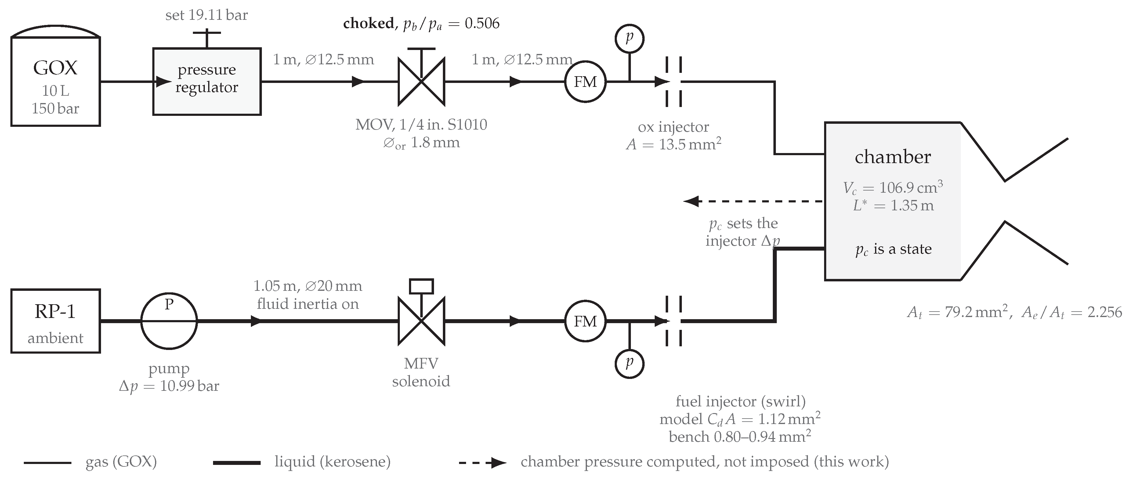
Figure 2.
Fuel injector cold-flow calibration. (a) Measured mass flow against with the fitted effective discharge area and the value carried by the model; the fit has . (b) Parity plot, dotted lines at .
Figure 2.
Fuel injector cold-flow calibration. (a) Measured mass flow against with the fitted effective discharge area and the value carried by the model; the fit has . (b) Parity plot, dotted lines at .
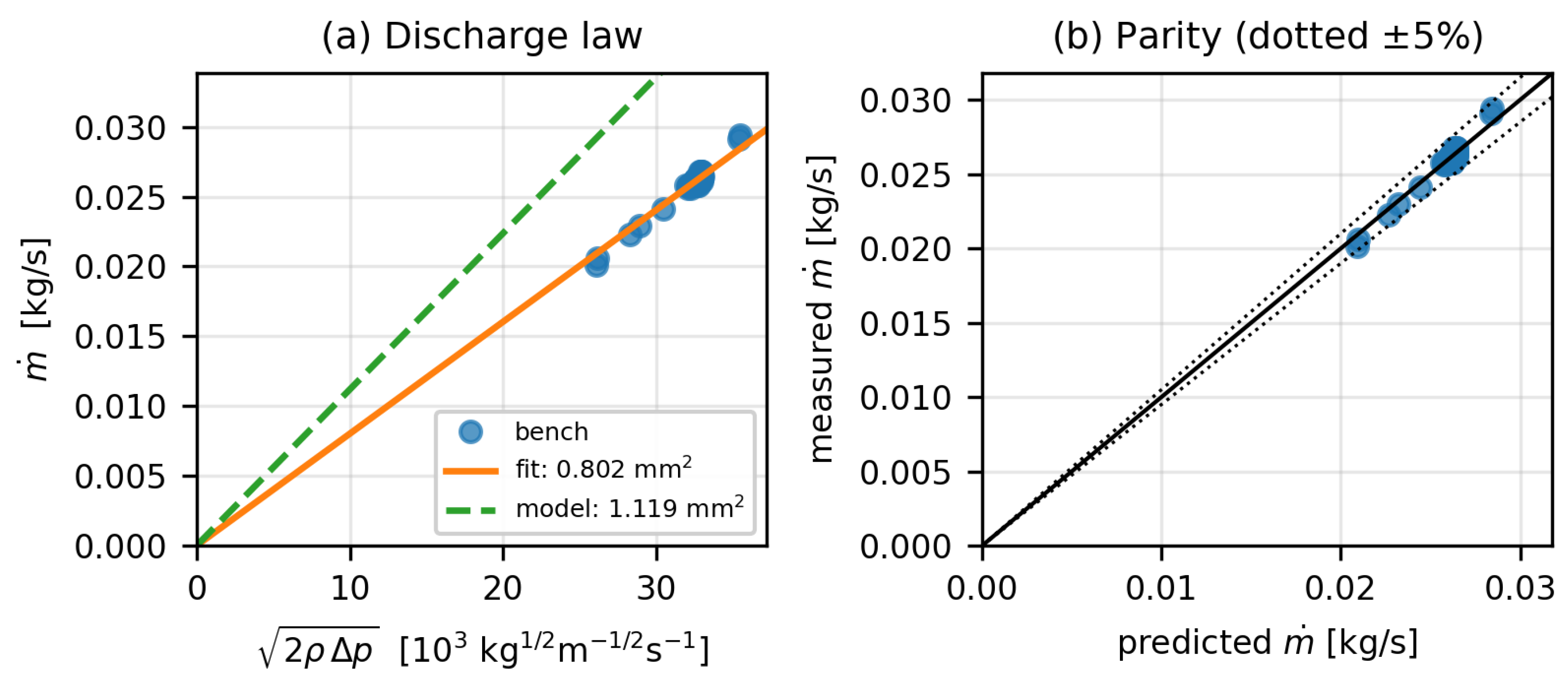
Figure 4.
Open-loop (dashed) and coupled (solid) predictions of the four quantities compared in Table 3: (a) chamber pressure, (b) mass flow, (c) mixture ratio, (d) thrust. The open-loop chamber pressure is an input and holds at its prescribed value; the coupled chamber pressure is a result. Dotted lines in (b) and (c) mark the design values.
Figure 4.
Open-loop (dashed) and coupled (solid) predictions of the four quantities compared in Table 3: (a) chamber pressure, (b) mass flow, (c) mixture ratio, (d) thrust. The open-loop chamber pressure is an input and holds at its prescribed value; the coupled chamber pressure is a result. Dotted lines in (b) and (c) mark the design values.
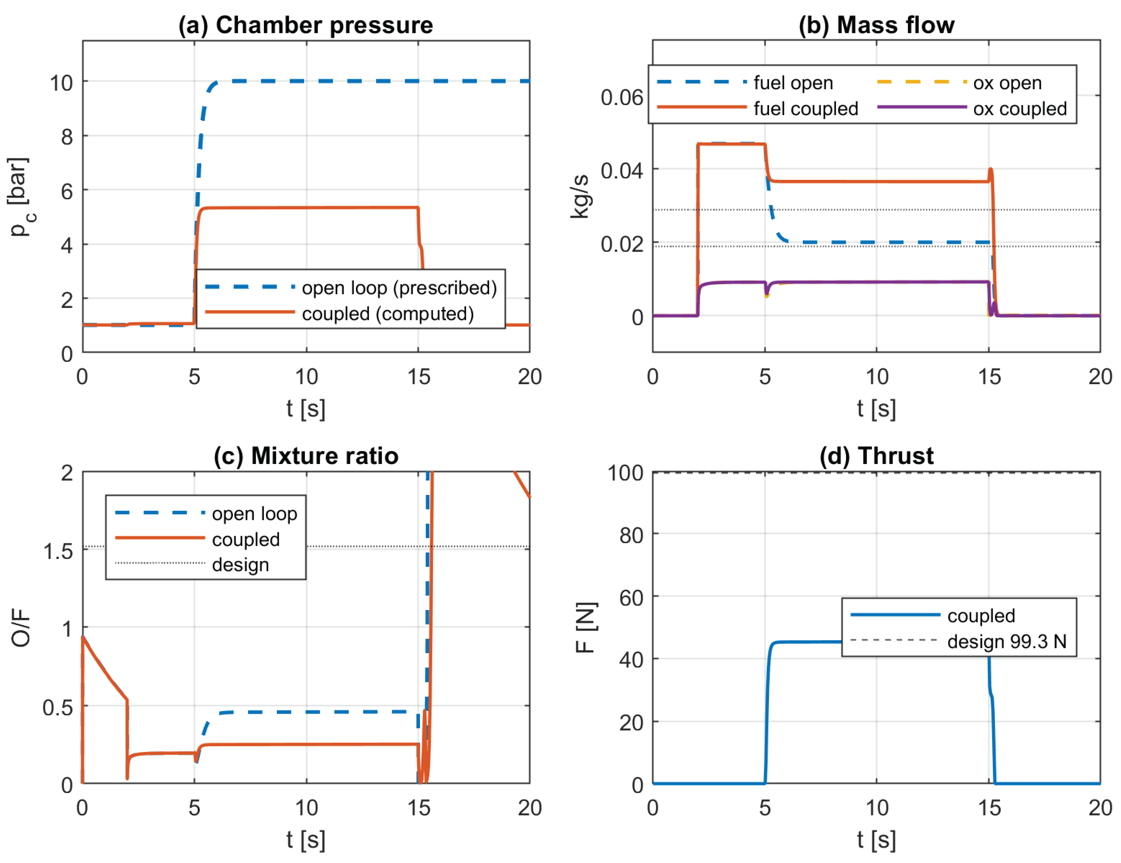
Figure 5.
Quantities available only from the coupled model. (a) Injector stiffness for both circuits against the 20 design target; the fuel injector settles at 125 and the oxidiser at . (b) Chamber temperature, which reaches only 828 at the fuel-rich operating point.
Figure 5.
Quantities available only from the coupled model. (a) Injector stiffness for both circuits against the 20 design target; the fuel injector settles at 125 and the oxidiser at . (b) Chamber temperature, which reaches only 828 at the fuel-rich operating point.
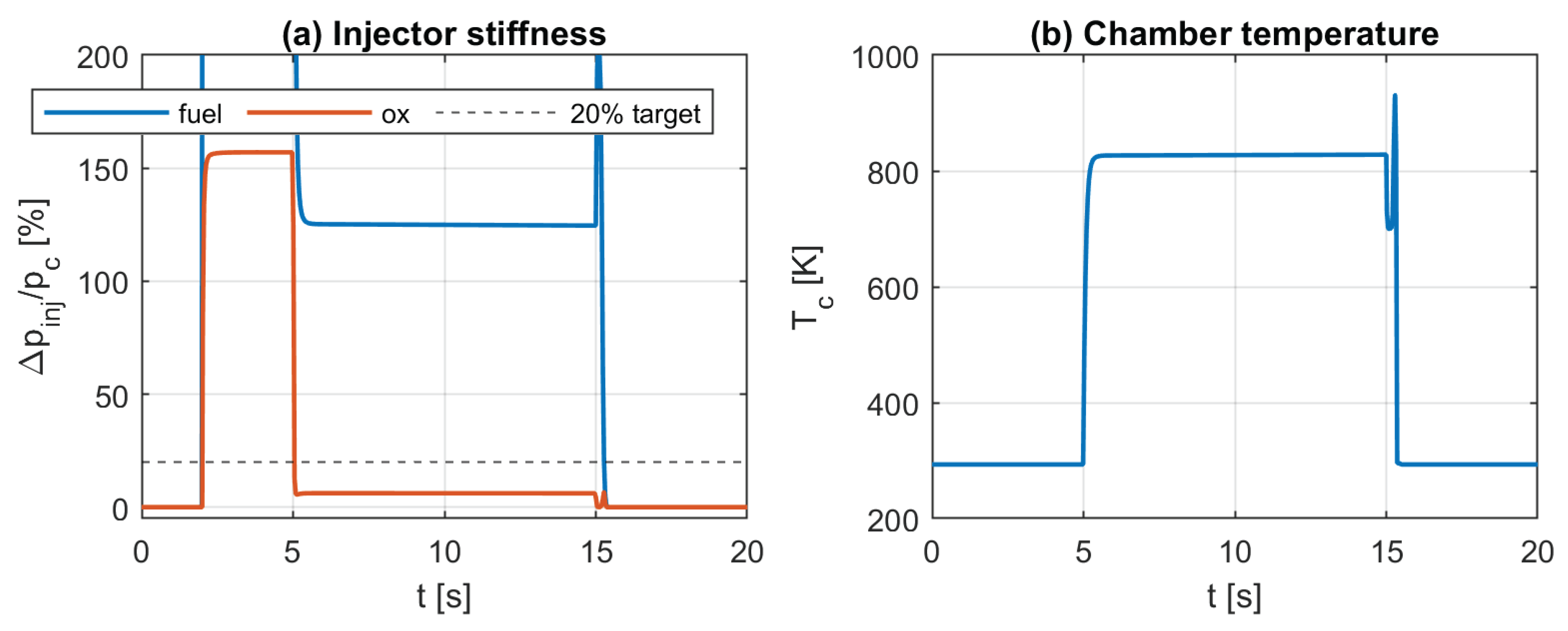
Figure 6.
Resolved ignition transient. (a) Chamber pressure rise. (b) Feed-system response to it: both flows fall as the chamber back-pressures the injectors, the oxidiser recovering as the gate valve rechokes.
Figure 6.
Resolved ignition transient. (a) Chamber pressure rise. (b) Feed-system response to it: both flows fall as the chamber back-pressures the injectors, the oxidiser recovering as the gate valve rechokes.
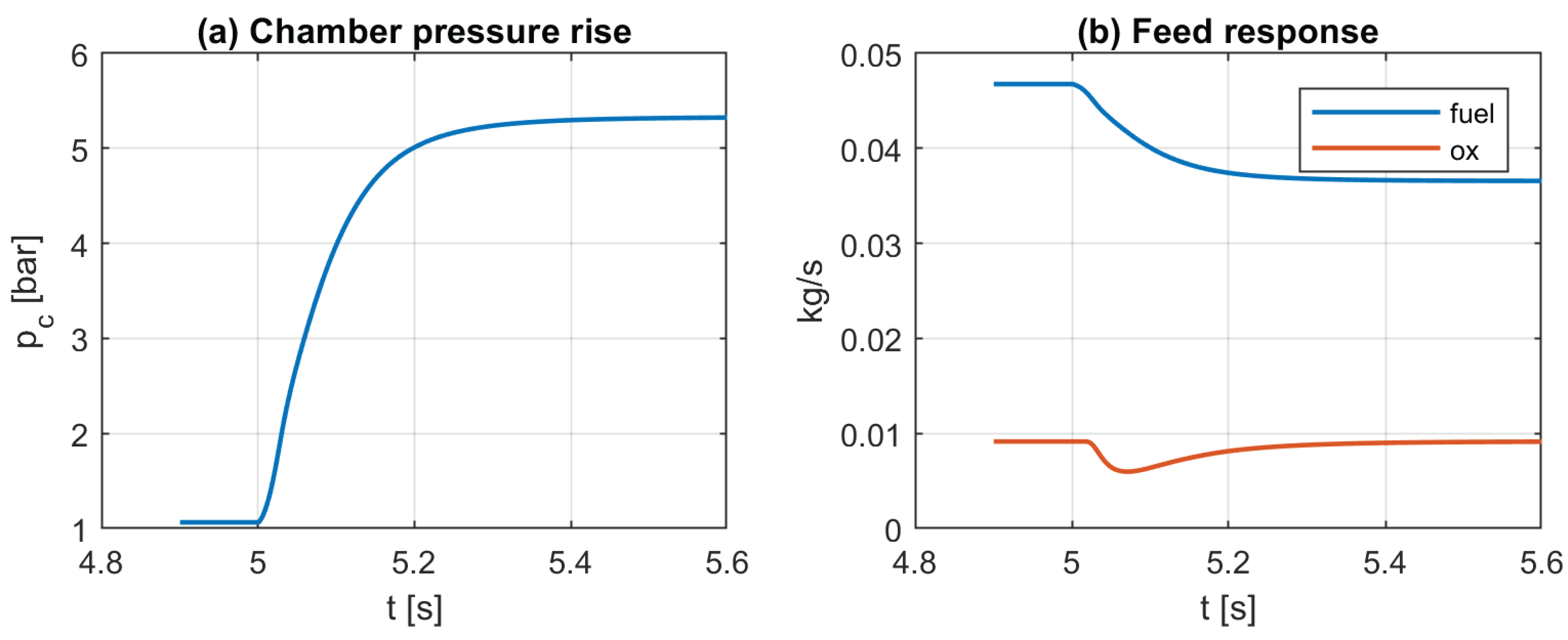
Figure 7.
Shutdown blowdown. Closing the fuel valve extinguishes the chamber through the combustion gate of Equation (6); the decay is the physical emptying of the chamber volume, not a scripted ramp.
Figure 7.
Shutdown blowdown. Closing the fuel valve extinguishes the chamber through the combustion gate of Equation (6); the decay is the physical emptying of the chamber volume, not a scripted ramp.
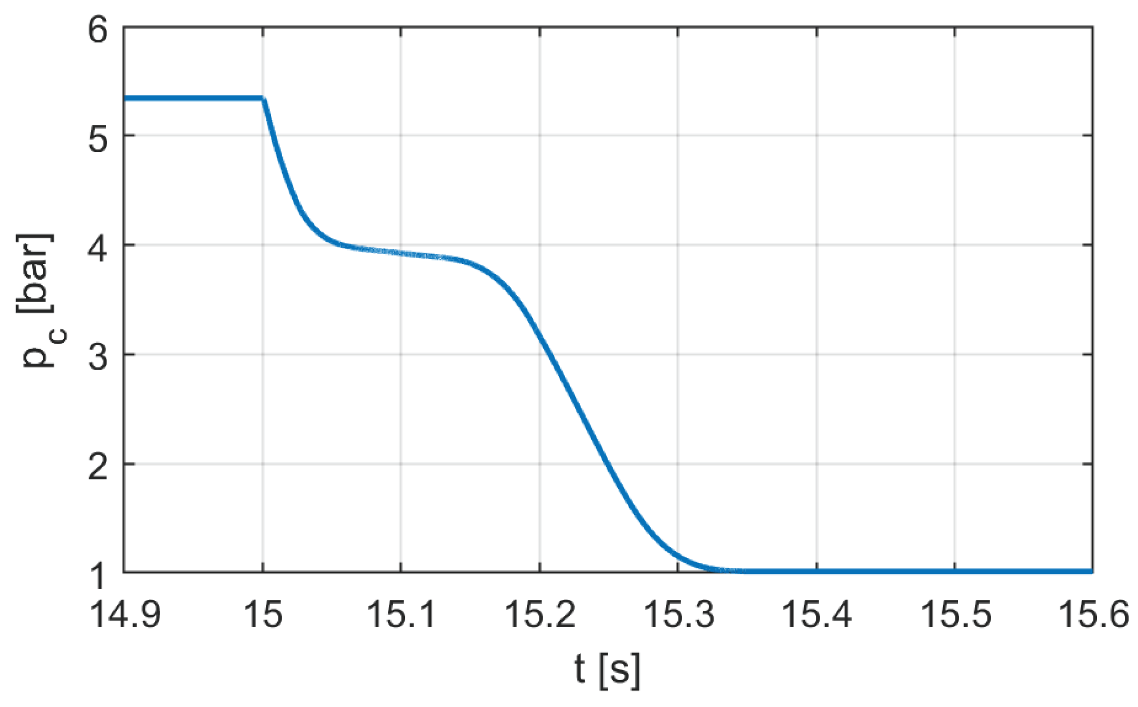
Figure 8.
Mechanism separation at the as-built operating point, where the fuel injector stiffness is 125. Freezing the thermochemistry removes the oscillation entirely; removing fluid inertia does not change it. The two -live curves are coincident.
Figure 8.
Mechanism separation at the as-built operating point, where the fuel injector stiffness is 125. Freezing the thermochemistry removes the oscillation entirely; removing fluid inertia does not change it. The two -live curves are coincident.
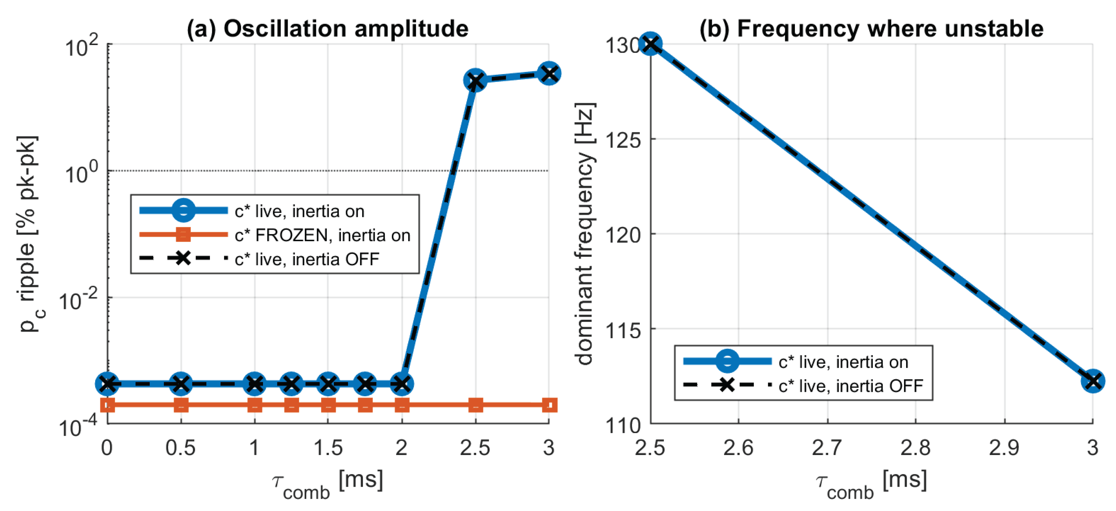
Table 1.
Fuel injector effective discharge area. Confidence intervals are bootstrap estimates of fit precision and exclude systematic instrument uncertainty.
Table 1.
Fuel injector effective discharge area. Confidence intervals are bootstrap estimates of fit precision and exclude systematic instrument uncertainty.
| Source | (mm2) | Implied 1 | |
|---|---|---|---|
| Bench, | 0.802 [0.800, 0.804] | 0.9625 | 0.577 |
| Bench, | 0.937 [0.935, 0.940] | 0.9481 | 0.675 |
| Model, as built | 1.119 | — | 0.806 |
1 On the documented geometric area of ().
Table 2.
Coupled model with the bench-calibrated fuel injector.
| (mm2) | (kg/s) | (kg/s) | O/F | (bar) | F (N) |
|---|---|---|---|---|---|
| 1.119 (model) | 0.03652 | 0.00921 | 0.252 | 5.34 | 45.4 |
| 0.937 () | 0.03157 | 0.00921 | 0.292 | 4.90 | 40.2 |
| 0.802 () | 0.02768 | 0.00921 | 0.333 | 4.55 | 36.0 |
Table 3.
Steady operating point, –.
| Open loop | Coupled | Design | |
|---|---|---|---|
| (kg/s) | 0.02005 | 0.03653 | 0.01898 |
| (kg/s) | 0.00917 | 0.00921 | 0.02884 |
| O/F | 0.458 | 0.252 | 1.520 |
| (bar) | 10.00 1 | 5.34 | 10.0 |
| (K) | — | 828 | 2575 |
| F (N) | 58.0 2 | 45.4 | 99.3 |
| , fuel (%) | 20.1 | 125 | ∼20 |
| , ox (%) | 1.75 | 6.2 | ∼20 |
1 Prescribed, not predicted. 2 Computed with a fixed inconsistent with the predicted mixture ratio.
Table 4.
Critical combustion lag and chug frequency from Equation (11), at the design operating point.
Table 4.
Critical combustion lag and chug frequency from Equation (11), at the design operating point.
| (%) | (ms) | (Hz) | |
|---|---|---|---|
| 5.0 | 0.252 | 0.89 | 210 |
| 7.5 | 0.378 | 1.50 | 165 |
| 10.0 | 0.504 | 2.37 | 125 |
| 12.5 | 0.630 | 3.63 | 92 |
| 15.0 | 0.756 | 5.69 | 66 |
| 17.5 | 0.882 | 10.21 | 41 |
| ≥19.8 | ≥1.0 | unconditionally stable | |
Table 5.
Chamber pressure ripple (% peak-to-peak, detrended) and dominant frequency.
| Configuration | 3 | ||
|---|---|---|---|
| live, inertia on | 0.00043 | 26.41 (130.0 Hz) | 34.03 (112.3 Hz) |
| frozen, inertia on | 0.00020 | 0.00020 | 0.00020 |
| live, inertia off | 0.00043 | 26.20 (130.0 Hz) | 33.76 (112.3 Hz) |
Disclaimer/Publisher’s Note: The statements, opinions and data contained in all publications are solely those of the individual author(s) and contributor(s) and not of MDPI and/or the editor(s). MDPI and/or the editor(s) disclaim responsibility for any injury to people or property resulting from any ideas, methods, instructions or products referred to in the content. |
© 2026 by the authors. Licensee MDPI, Basel, Switzerland. This article is an open access article distributed under the terms and conditions of the Creative Commons Attribution (CC BY) license (http://creativecommons.org/licenses/by/4.0/).
Copyright: This open access article is published under a Creative Commons CC BY 4.0 license, which permit the free download, distribution, and reuse, provided that the author and preprint are cited in any reuse.