
Submitted:
24 August 2026
Posted:
25 August 2026
You are already at the latest version
Abstract
We investigate radiative transfer in strongly magnetized electron–ion plasmas relevant to magnetar atmospheres, where surface magnetic fields exceed B ≳ 1014 G. Extending the conventional cold-plasma approximation, we incorporate finite-temperature effects into the dielectric tensor and derive temperature-dependent polarization eigenmodes, electron scattering opacities, and free-free absorption opacities for a fully ionized hydrogen plasma. We show that thermal corrections significantly modify photon propagation and polarization evolution, smoothing resonance features through Doppler broadening and Landau damping and altering mode conversion between the ordinary (O) and extraordinary (X) polarization states. The resulting opacities differ substantially from cold-plasma predictions, particularly near vacuum and electron cyclotron resonances. Using these modified opacities, we calculate the emergent radiation spectra and find that finite-temperature effects enhance low-energy emission, broaden resonance structures, and modify the high-energy spectral tail through polarization-dependent Comptonization. Our results demonstrate that thermal effects play a crucial role in shaping the spectral and polarization properties of magnetar radiation and provide a more realistic framework for modeling thermal emission from highly magnetized neutron stars.
Keywords:
neutron stars
; electron scattering opacity
; radiation modes
; free-free opacity
1. Organization of the Article
The paper is organized as follows. Section 1 contains a brief introduction of the magnetar environment and current gap need to address. In Section 2, we develop the theoretical framework for incorporating finite-temperature effects into the dielectric properties and radiative transfer equations of strongly magnetized plasmas. Section 3 examines the influence of thermal corrections on the polarization eigenmodes. In Section 4, we present the resulting electron-scattering and free-free absorption opacities and compare them with the corresponding cold-plasma predictions. Section 5 discusses the emergent flux spectra obtained from the radiative transfer calculations and summarizes our main conclusions.
2. Introduction
The thermal radiation emitted from the surfaces of isolated neutron stars (NSs) provides one of the most powerful probes of their physical properties and evolutionary history. Over the past two decades, thermal surface emission has been detected from several classes of isolated NSs, including radio pulsars, radio-quiet NSs, anomalous X-ray pulsars (AXPs), soft gamma-ray repeaters (SGRs), and young compact objects associated with supernova remnants [1,2,3]. The interpretation of these observations critically depends on the properties of the thin atmospheric layer that covers the stellar surface. Although this atmosphere typically has a scale height of only –10 cm and densities of -100 g , it strongly modifies the emergent radiation through absorption, scattering, and polarization processes [4]. Consequently, a detailed understanding of radiative transfer in strongly magnetized NS atmospheres is essential for extracting reliable constraints on stellar masses, radii, surface compositions, and magnetic field strengths from observational data [5,6,7].
Particularly important are magnetars, whose surface magnetic fields can exceed G. Such extreme fields fundamentally alter atomic structure, plasma properties, and radiative processes, leading to substantial deviations from blackbody emission. Recent observational analyses have shown encouraging agreement between high-field atmosphere models and measured X-ray spectra [3,8], while theoretical studies have demonstrated the potential of atmospheric modeling to constrain the underlying physics of NS interiors and magnetospheres [4,9]. Therefore, comprehensive investigations of thermal emission from magnetized atmospheres are crucial for understanding the composition, structure, and physical conditions of magnetars.
The emergent spectrum depends sensitively on the atmospheric composition, equation of state, and radiative opacities. Even when fallback material or subsequent accretion is present, gravitational stratification is expected to produce a nearly pure hydrogen atmosphere [10]. Photons decouple from matter at Thomson depths of approximately , making the accurate determination of opacity sources a central aspect of atmosphere modeling [6]. Significant progress has been achieved over the past several decades. The first non-magnetic NS atmosphere models were developed by Romani [11], followed by more sophisticated calculations incorporating improved opacity data from the OPAL project for hydrogen, helium, and iron compositions [12]. Subsequent studies extended these models to include magnetic fields, initially focusing on fully ionized hydrogen plasmas with field strengths of - G [13]. These investigations demonstrated that light-element atmospheres produce spectra that differ substantially from simple blackbody predictions.
Early attempts to model magnetic NS atmospheres were pioneered by Miller [13]; however, those calculations included only bound-free opacities and employed simplified treatments of polarization. Later studies incorporated electron scattering and free-free absorption processes, leading to more realistic spectral predictions [12]. The resulting magnetic spectra were found to be harder than blackbody spectra while remaining softer than their non-magnetic counterparts at high energies [12]. Despite continued advances, the treatment of heavy-element atmospheres in strong magnetic fields remains challenging because of the complexity of atomic structure and radiative transfer under such extreme conditions [12]. Nevertheless, both hydrogen and iron atmosphere models have been successfully applied to observations of radio pulsars and radio-quiet NSs, yielding valuable constraints on stellar parameters [15].
The discovery of magnetars and the accumulation of high-quality X-ray and -ray observations have significantly advanced the study of radiative processes in strongly magnetized plasmas [16]. Early atmosphere calculations generally assumed fully ionized, non-magnetic plasmas and employed classical opacity prescriptions [17]. As the importance of magnetic fields became increasingly evident, theoretical efforts incorporated polarization-dependent opacities and magnetically modified radiative transfer through the cold plasma approximation [20]. This framework was further refined in the influential works of Ho and Lai [1,4,6] and, more recently, by Zhang and collaborators [3], who included effects such as partial ionization and vacuum polarization.
Despite their success, most existing magnetar atmosphere models continue to rely on the cold plasma approximation, which neglects the thermal motion of electrons. While this approximation is often adequate for relatively cool NS atmospheres, its validity becomes increasingly questionable in hot magnetar environments, where thermal effects can significantly modify the dielectric response of the plasma and, consequently, the radiative opacities. The omission of finite-temperature corrections may therefore introduce systematic uncertainties into theoretical predictions of polarization properties and emergent spectra.
Motivated by these considerations, we investigate the influence of finite-temperature effects on radiative transfer in strongly magnetized magnetar atmospheres. We derive analytical expressions for electron-scattering and free-free absorption opacities that incorporate thermal corrections beyond the cold plasma limit. Our formulation includes relativistic thermal broadening and temperature-dependent modifications to polarization-dependent opacities. To quantify the impact of these effects, we numerically solve the coupled radiative transfer equations for the ordinary (O) and extraordinary (X) polarization modes in a fully ionized hydrogen plasma confined by superstrong magnetic fields ( G). We then compare the resulting opacities and emergent spectra with those obtained under the conventional cold plasma approximation.
Our calculations demonstrate that finite-temperature effects produce measurable modifications to both the opacity structure and the emergent radiation field. In particular, thermal corrections soften the high-energy tail of the emergent spectrum relative to cold-plasma predictions and alter the angular beaming pattern of the emitted radiation. These effects are potentially important for the interpretation of phase-resolved observations from modern X-ray and -ray observatories such as XMM-Newton and Fermi [21]. By providing a more physically realistic description of radiative processes in magnetar atmospheres, our results offer a framework for improving the consistency between theoretical models and observational data.
3. Theoretical Work-Frame
The dynamics of a magnetized thermal plasma in the vicinity of a magnetar are described by the relativistic fluid equations coupled with Maxwell’s equations. For each plasma species (s), the governing equations are given by
together with Maxwell’s equations,
Equation (1) represents momentum conservation, including the Lorentz force and pressure-gradient terms. Equation (2) is the continuity equation, while Equation (3) describes the evolution of plasma pressure, where denotes the heat-flux vector. Equations (4) and (5) correspond to Faraday’s and Ampère’s laws, respectively. The subscript (s) identifies the plasma species, with (s=e) and (s=p) denoting electrons and positrons. The mass density is defined by , and is the relativistic Lorentz factor. In this work, we consider a thermal electron-positron pair plasma, which provides an appropriate description of the magnetospheric environment of magnetars. The objective is to derive a generalized dispersion relation for electromagnetic waves propagating in a strongly magnetized thermal plasma and to investigate the effects of finite temperature on wave propagation. Following the standard linear perturbation procedure [18,19], all physical quantities are decomposed into equilibrium and first-order perturbed components. Assuming plane-wave perturbations of the form and neglecting the heat-flux contribution, Eqs. (1)-(5) reduce to
where is the cyclotron frequency of species s, where s=-e for electrons and s=+e for positrons. Retaining the sign of the particle charge is essential for correctly describing the off-diagonal (Hall) component of the dielectric tensor in an electron–positron pair plasma. The relativistic effective inertia is adopted in the linearized fluid equations. Subscript 1 denotes the first-order perturbed quantities. Using the linearized continuity Equation (9) and pressure equations (10), the density and pressure perturbations are first expressed in terms of the perturbed fluid velocity. These relations are then substituted into the linearized momentum equation Equation (8) to obtain the velocity response of each plasma species. Consequently, the perturbed velocity can be written as,
where denotes the inverse of the response tensor , is the mobility of the fluid, and second-rank response tensor is defined as .The isotropic thermal correction is represented by the coefficient , which originates from the pressure-gradient term in n Equation (8) after eliminating the density and pressure perturbations using the continuity and pressure equations, Equation (9) and (10), respectively. The tensor represents the anisotropic thermal correction arising from the coupling between the finite-temperature pressure response and the background magnetic field. Where, is the refractive index vector is used to defined retractive index that contains the isotropic and anisotropic fluid pressure as given below,
It should be noted that is the angle between the wave vector and the background magnetic field (the magnetic field of the magnetar). The mobility has also second ordered thermal corrections ), but we are considering first order thermal corrections ) in the present theoretical framework due to negligible contribution from higher moments like heat flux. Here, we are taking into account only electron-positron thermal pair plasma. The second relativistic parameter is (where is the thermal speed of the particle) will be used through out in the manuscript.To derive the wave equation [19], the perturbed current density is obtained by summing the contributions from all plasma species, . Using the linear velocity response , the current density becomes , the constitutive relation for the current density is given as
Together with Maxwell’s equations, yielding , where, is the conductivity tensor . Now we can use Equation (9) and (10) to present wave equation of electromagnetic waves travelling in thermal plasma fluid given as
here, the product of makes the linear velocity response and the conductivity tensor becomes , therefore, the dielectric response tensor gives , where, is the positron and electron plasma frequency. The generalized dispersion relation for the thermal electron-positron plasma is written as
3.1. Limiting Case: Cold Plasma
In the limit of ,the dielectric tensor reduces to the cold-plasma limit and describes the propagation characteristics of electromagnetic waves in the electron–positron pair plasma, the dielectric tensor becomes
and
Thus, the dispersion relation of the electromagnetic waves in a cold magnetized electron-positron plasma can be written as
where, , and are the coefficient of the quadratic refractive index equation with analytical solution gives the explicit dispersion relation for the cold plasma modes
one can retrieve the earlier results of cold plasma modes in the magnetosphere of a magnetar [4]. The unit polarization vector has been defined in order to derive the dispersion relation for particular photon mode propagation as given in Ref. [4]
where, the subscript j represent the index of the mode, for instance, j=1 and j=2 is for the extraordinary mode X and ordinary mode O, respectively. The polarization vector is obtained by solving Equation (21), yields
In above expression, is the polarization parameter. There are two types of photon modes, ordinary (O-mode) and extraordinary (X-mode). When , the X-mode has and its electric field component E is mostly perpendicular to the plane whilst the O-mode has and is polarized along the plane. This traditional approach of identifying photon modes is appropriate. The primary advantage of this classification is that the X- and O-modes interact with matter in very different ways. The X-mode opacity is greatly lowered (by a factor of the order ) from the zero-field value, whilst the O-mode opacity is essentially unaffected by the magnetic field in this limit of polarization parameter . Nevertheless, near , the classification of X- and O-modes becomes unidentified. In fact, when crosses through at the resonance wave number, it becomes discontinuous (and changes sign), as demonstrated in Ref. [4]. Take into consideration the propagation of a planar monochromatic electromagnetic wave with wave vector along z-direction, while, in the yz plane, let be a uniform static magnetic field that forms an angle theta with z-axis in Cartesian coordinate system. Whereas, in the xy plane, the electric field vector of the normal modes, , spans on an ellipse. It is conventional to refer to the as the “extraordinary mode” and the as the “ordinary mode”, typically, there is also an electric field in the z direction; for instance Equation (7) of CANUTO [23]. The ratio between the components and , in the two modes is , where, and (Here, and ), K is the polarization parameter and is the index of refraction for the particular mode. When waves propagate parallel to the magnetic field , the two waves are circularly polarized with opposite helicities, such that the component is in phase with and out of phase with and hence, and . However, if wave is normal to , and resulting linear polarization of the propagating modes in xy-plane. The plasma contribution to the dielectric tensor for a cold electron-ion plasma can be expressed in the rectangular coordinate system with B along z-direction as , and . The electrons and ions are linked together by collisions (with the collision frequency ei), in accordance with Ginzburg [? ]. Extending Ginzburg’s observations by include the radiative dampings of ions and electrons, the dielectric tensor’s plasma contribution in the coordinate system xyz with B along z can be calculated by and where and are the normalized damping rates for respective speices as given in Ref.[? ]. Moreover, is definition used in Equation (18). A correction to the dielectric tensor is provided by vacuum polarization [? ], where I is the unit tensor and is the unit vector along B. Inclusion of vacuum polarization cause alteration in the magnetic permeability tensor of an electromagnetic wave and magnetic field is connected to its magnetic induction as , where and are vacuum polarization coefficients as given in Ref. [? ].
3.2. Thermal Plasma Case
For the thermal case, we obtained the relation of plasma fluid waves with .From Equation (9) and (10), one can obtain relation for perturbed number density and pressure as and , respectively. Substituting these experession into Equation (8) gives the velocity response as given in Equation (13). However, now , where, (here, is the dimensionless thermal parameter. The isotropic and anisotropic thermal corrections contained in the dielectric tensor are then obtained from the first-order expansion . The dielectric tensor contains . To derive an explicit relation for the thermal case that will be valid over the entire frequency range, let us present a modified frequency given as
where, here, is redefined due to replacement of . The present analysis retains only first-order (). Accordingly, the perturbative expansion remains valid provided that . The analytical expansion is not evaluated exactly at the singular resonance point. Instead, the numerical analysis is restricted to parameter regimes where the perturbation remains well behaved, and the first-order approximation is self-consistent. All these amendments are up to to first order in thermal wave propagation in the plasma fluid. The plasma species satisfies the relation and describes a particular propagation regime of wave propagation, here . For instance, in the range , on the other hand, the thermal plasma made up of electron-positron pairs which is a valid consideration inside the magnetosphere of the magnetar [8], the validity condition still holds or . Using the arguments discussed above and the modified modes of wave propagation, we can derive the dispersion relation for the magnetized electron-positron thermal plasma modes and the modified dielectric tensor can explicitly be written as,
.
Along together with the additional matrix due to finite thermal effects of the electron-positron pair plasma waves propagation in the presence of magnetic field as described in the environment of the magnetar.
The coefficients are obtained by evaluating the elements of after retaining terms up to first order in the thermal parameter . These coefficients therefore represent the thermal modification of the cold-plasma response and constitute the elements of the effective dielectric tensor used to derive the cubic dispersion relation. Thus, the dispersion relation of the electromagnetic waves in a thermal magnetized electro-positron plasma can be written as,
where, are the coefficient of the cubic refractive index n whose analytical solution yields the explicit dispersion relation for the thermal plasma electron-positron modes.
where and are the coefficient of the roots. The dispersion relation Equation (23) can be solved analytically for arbitrary angle as contrast to numerically computing the implicit dispersion relation Equation (19) using the cold plasma approximation. Given that all first-order terms are retained , the explicit thermal dispersion relation is not only useful but also appropriate because it replicates the cold plasma dispersion relation [4].The dispersion relation is derived in the first-order thermal approximation. Consequently, the calculated eigenmodes describe the propagation characteristics of electromagnetic waves in a magnetized thermal electron–positron pair plasma. The thermal corrections modify the refractive index, resonance frequencies, cutoff conditions, and polarization properties through changes in the dielectric response of the plasma.
Figure 1.
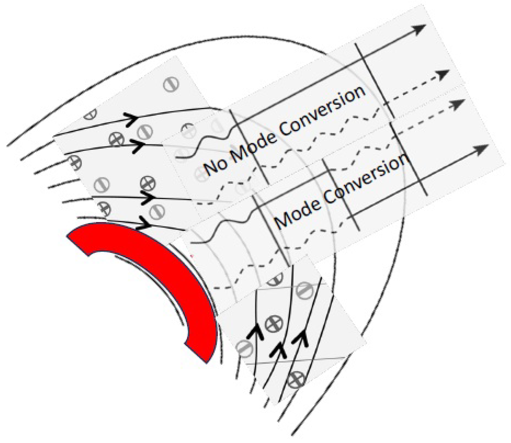
A schematic diagram for the emission of thermal radiation from the surface of NS surrounded with relativistic plasma.
Figure 1.
A schematic diagram for the emission of thermal radiation from the surface of NS surrounded with relativistic plasma.
4. Opacity and Flux Calculations
4.1. Electron Scattering Opacity
The identical unit vector of mode for the electric field is . Since the j mode can scatter into ordinary and extraordinary waves, the two potential scattered waves are included over l, and the angle between the wave vector and the dispersed Poynting vector is known as the scattered angle " (please see Figure 2 of Ref. [? ]). For scattering from to , the differential cross section is (where, is the power flux of incident radation). The net mean power scattered from above Equation (46) given as
here, is the components of scattered electric field vector of radiation in terms of incident wave as given in Equation (A6) of Ref.[? ]. The differential cross section is compatible with and may be expressed up by the subsequent formal definition (despite its mathematical complexity):
where is related to dielectric tensor of the medium, is the transverse polarized vector, e and are incident and scattered polarizations of electric field vector , respectively. In fact, the mechanism of radiation scattering is found in Equation (47). When an electro-magnetic wave encounters charged particles, they create polarization currents that generate secondary radiation sources. Because of the significant anisotropic character of the medium response, the resulting radiation is also anisotropic when a strong magnetic field is present. Significantly, the structure of the propagation modes e and that the medium permits determines the particular characteristics of the results. As was demonstrated in the previous section, it is actually important to maintain an independent track of the intent of the polarization modes, which frequently contain all of their reliance on the incident and final photon angles. The plasma modes e and e must still be expressed in the coordinate frame with the z axis along B in order to calculate the cross section. Equation (10) of Ref. [? ] provides an appropriate rotation of coordinates for propagation along wave vector . Hence, the term in Equation (48) can be written as
The angles of the incident photon k and the scattered photon through the polarization vectors influences the differential cross section. The low-frequency behavior of differential cross section, which is independent of the initial and scattered azimuthal angle of and with respect to the wave vector and magnetic field plane vectors, may now be readily determined. This expression implies that the corresponding cross section of those propagation modes with e perpendicular to the plane will be drastically reduced in regard to the Thomson cross. It will be helpful to provide information about the integrated cross sections because it provides a clearer picture of the final result. By integrating Eqs. (48) and (49) over the angles of the scattered photon, we may determine the integrated “partial" cross section into a final mode or for an incident photon of polarization . The integrated cross section can be written as
here, is an angle integrals of the final polarization are used to define the constant vector, numerical values of this constant are given in Table 1 of Ref. [? ] . For case of transverse polarized mode completeness property is fulfilled, hence, and from which semi-transverse limit or , and can be concluded. The validity of Equation (50) is broader. Consequently, it is important to note that Equation (50) can be directly derived from Equation (49) by using a matrix algebra in the same limit of semi-transverse waves. The general form of integrated cross section can be defined as follows,
where, is polarization tensor depend on the permittivity of medium. An intuitively appealing explanation of results is suggested by the fact that is proportional to the polarization current that the incident wave induces in the medium. The polarization components perpendicular to magnetic field are diminished at low frequencies , resulting in outcomes that significantly rely on the polarization modes. The cross section is significantly reduced if , for instance see Equation (10) of Ref. [20]. Whereas, those modes with a strong component scatter at about the typical Thomson cross section. One circular polarization, in which the electric vector rotates in the same direction as the gyro motion of electron, becomes resonant at frequencies close to the cyclotron frequency. The cross section of the extra-ordinary mode reaches a sharp maximum at as a function of frequency. The well-known relation can be used to derive a completely general equation for the total cross section from the imaginary component of the refractive index as given in Ref.[20,21,22]. Using the rotating-coordinates form of the polarization vector again and taking into account the radiation-damping, we so discover
where, . The entire cross section of a photon beginning in mode can be expressed in this generalized form of Equation (33). In the limit of semi-transverse propagation, earlier results can be retrieved [19,20]. Where, is the imaginary part of the refractive index of the medium. Through its projection on the rotating frame with the z-axis along B, the normal mode polarization vector determines the radiative opacities. The cyclic components of polarization vector is given as [4]
where has been discussed in pervious section in detail. Hence, the electron scattering opacity for the two component plasma (i.e., electron-positron) of the mode j can be explicitly presented as [4,24]
is the scattering coefficient in a un-magnetized plasma and is the line width of cyclotron resonance, is number density of the electron and is the mass density of electron-ion thermal plasma.
4.2. The Electron Free-Free Opacity
The mobility of electrons on the stellar surfaces is dominated by the enormous magnetic fields (, i.e., ) that surround neutron stars. The Schrodinger equation for the dynamics of electron in a uniform, static magnetic field is presented as [24]
where is the Dirac magnetic moment. Equation (55) is presented in cylindrical polar coordinate , the magnetic field is taken into account in the z-axis, and the associated vector potential is . The solution of Equation (55) is presented as [24]
where , F is the hyper-geometric function, L is the normalized length in the direction and is the normalization constant. The corresponding eigenvalues of the energy (here, S is the spin of the electron) give for , which is much larger than the normal value of in the magnetar magnetosphere under the radiative cooling process. It is well-known that the electron distribution function determines the photo-absorption coefficient in a given medium. The phase space of electron transforms into a special combination of discrete Landau levels when a huge magnetic field is applied. Radiative excitation and de-excitation, or cyclotron absorption and emission, are the primary mechanisms governing the occupation of the transversal different levels. The Landau levels are typically populated by these processes. The coefficient of absorption is given as
is the free free opacity of a nonmagnetic plasma, where is the de-excitation collisional rate, Z is the ion charge, and are the electron and ion number densities, respectively. There are two typical modes of high-frequency wave propagation in a magnetized plasma as discussed in above section. If these modes have a substantial relative phase shift along a single photon mean free path, they propagate independently in an optically thick medium. An induced polarization current density (where is the electric field vector of mode and is the susceptibility tensor of the medium) is present when a wave of angular frequency and mode propagates in a medium. Both of collisional and radiation damping have an effect on this current. As mentioned in the previous subsection, the first of these losses is directly related to the total scattering coefficient, whereas the second is related to the bremsstrahlung coefficient, which is dependent on the angle between the magnetic field and the direction of propagation. The ratio of the collision and radiation damping frequencies can exhibit simple behaviors, despite the fact that both variables are very anisotropic and polarization sensitive. Numerous authors have attempted to calculate free absorption using QED calculation . The free free opacity in magnetized plasma can be expressed as [24].
where is the minimal final velocity of the electron. The mean value of the tensor G summarizes the strong dependency of the absorption coefficient on the polarization vector e in the magnetized plasma environment. The free-free absorption coefficient may be expressed as [24] at the simplest degree degree of approximation.
In above Equation (40), the tensor G is expended in rotating coordinates . The averages of the microscopic (velocity and Landau number dependent) Gaunt factors can be used to express these generalized Gaunt factors , which are dependent on the electron distribution function as given below,
The -function admits one of the v-integrations to be evolved and in which remains constant to fulfill law of conservation of energy. The integral of microscopic Gaunt factors [? ] can be express as
where , and are the matrix elements as defined in [24].The velocity dependent shape and collision functions must be numerically integrated in a complex way in order to obtain precise values for the Gaunt factors . Nevertheless, effective approximation formulas can be developed. For instance, the Gaunt factors are simply calculated using the averaged Coulomb matrix elements and to determine the contribution of the lowest Landau level. The Gaunt factors are subsequently given as
and , where . It is possible to predict as to whether any of these characteristics could be observed in gamma burst spectra. According to model calculations, the scattering cross section determines the line shape in the optically thick scattering-dominated regime. However, if the field is homogeneous in the radiating region, the sharp peaks in the free free emissivity could become rather noticeable in the optically thin scenario. The remarkably sharp lines observed in the spectra of some cosmic GRBs may be explained by a kinematic effect as discussed. The general form of electron free-free abosorption opacity is presented as [4]
Where, is the velocity averaged free-free Gaunt factor in the presence of magnetic field [20].
4.3. Flux Calculations
The radiative transfer of the Stokes parameters [19] decreases to that of the two modes (X- and O-mode) when the normal modes are roughly orthogonal and have a substantial relative phase shift across a mean free path, for instance at large Faraday depolarization. For the particular intensity of mode j, the Radiative Transfer Equation (RTE) is given as
where is the blackbody intensity and . Generally, when B is not along the surface normal at , the intensity depends on and the azimuthal angle for a given frequency and Thompson depth (where, is the Thompson scattering opacity in the absence of magnetic field), above RTE Equation (45) can be written as
Introducing and only computed for are correlated with the energy flux and mean specific intensity (for the non-magnetic example, see [? ]). Consequently, the RTE becomes [? ]
The zeroth-order moment of the transfer equation is obtained by integrating the RTE over the solid angle in order to determine the limitation imposed by radiative equilibrium.
and the specific flux of energy with given frequency is given as
A modified blackbody coherent (CC) spectrum with an incoherent (IC) end at the high-energy tail is most likely the resultant spectrum as the current observations [8] are suggested by subject to both CC and IC scattering. The two radiation processes mentioned can be taken into consideration to generate a parametrized function of the model-predicted spectrum. The Compton parameter (here, N is mean scattering number when a photon moves along a free path), which changes at different photon energy, determines whether the CC or IC dominates the radiation process. There are two regimes in which the flux can be calculated, contingent on the or . The CC is dominant when , and there is minimal variation in the energy of a scattered photon. The scattering and absorption of thermal photons are directly correlated with the specific intensity [20]as given below
where is the X/O polarized mode for electron scattering and , similar for for free free absorption (bremsstrahlung) opacities from plasma environment for E-mode and O-mode photons of in a thermal medium. The observed specific flux at a luminosity distance can be evaluated by taking Doppler boosting into consideration as [? ]
where, is the luminosity distance and the Doppler factor is denoted by D. In the second regime at , the IC dominates the radiation and energy is transferred to the photons from electron-positron pairs in the magnetized plasma. In this instance, the Wien law will immediately be implemented to the specific intensity as given below
where and are the coupling number density and coupling mass, respectively. While, N is the total number of particles and V is the volume of the radiation region. In a magnetized degenerate plasma, if photons are coupling with electron-positron pairs, the coupling number density factor may be substantial. At the observer, the specific flux is given as
.
5. Results and Discussion
5.1. Polarization Mode Conversion
The combined effects of plasma and vacuum polarization govern the dielectric properties of strongly magnetized neutron-star atmospheres. When these two contributions become comparable, a vacuum resonance occurs, leading to significant modifications in photon propagation and polarization states. In such environments, the extraordinary (X) mode is polarized perpendicular to the plane, whereas the ordinary (O) mode is polarized within the plane. For photon energies well below the electron cyclotron energy, both modes remain nearly linearly polarized.
As photons propagate through the inhomogeneous atmosphere, their polarization states evolve in response to local plasma conditions. If the density gradient is sufficiently gradual, the evolution proceeds adiabatically, allowing photons to remain on the same polarization branch while their modal properties continuously change across the vacuum resonance. Consequently, an X-mode photon can convert into an O-mode photon, or vice versa. Because the two polarization modes possess markedly different opacities, mode conversion plays a crucial role in determining the emergent radiation spectrum and polarization characteristics of magnetar atmospheres.
Using the polarization index , defined through the polarization eigenvectors of the dielectric tensor [24], we investigate the evolution of photon polarization over a broad frequency range extending from the infrared ( Hz) to the -ray regime ( Hz). Figure 2 illustrates the frequency dependence of the polarization parameter for representative plasma densities and magnetic field strengths characteristic of magnetar atmospheres.
The calculations reveal pronounced changes in the polarization state near the vacuum resonance frequency. For the strongest magnetic-field configuration ( G and ), a clear transition from X-mode to O-mode propagation occurs near Hz. Following this conversion, photons continue to propagate in the O-mode until reaching the electron cyclotron resonance frequency, , where an additional mode transition is observed. These results demonstrate that both vacuum and cyclotron resonances strongly influence the polarization properties of radiation emerging from strongly magnetized neutron-star atmospheres.
The calculations were performed using the transverse approximation (), an ideal hydrogen plasma equation of state, and surface gravity , corresponding to a canonical neutron star with mass and radius km. Two distinct resonance mechanisms are evident: (i) vacuum resonance arising from quantum electrodynamic birefringence of the vacuum in ultra-strong magnetic fields, and (ii) electron cyclotron resonance caused by resonant interactions between photons and gyrating electrons.
When finite-temperature corrections are incorporated into the dielectric tensor, the polarization behavior changes substantially. As shown in Figure 3, thermal effects smooth the sharp transitions predicted by the cold-plasma approximation. In particular, thermal broadening and Landau damping suppress intermediate mode-conversion features and eliminate abrupt cutoffs that are characteristic of cold-plasma models. Instead, the transition between polarization states becomes continuous, reflecting the influence of pressure gradients and thermal particle motions. The resulting behavior provides a more realistic description of radiative propagation in magnetar atmospheres and is expected to improve agreement with observational data [3].
5.2. Opacity Modifications
The frequency dependence of the electron-scattering opacity, , for the X- and O-polarization modes is shown in Figure 4 and Figure 5. In the cold-plasma approximation (Figure 4), the X-mode opacity exhibits a gradual increase at low frequencies, followed by a sharp enhancement near the vacuum resonance frequency. This feature corresponds to the conversion of X-mode photons into O-mode photons and reflects the strong coupling between polarized radiation and the magnetized plasma.
Beyond the vacuum resonance, the opacity enters a relatively smooth regime dominated by O-mode propagation. At higher frequencies, a second prominent feature appears at the electron cyclotron resonance, where photon-electron interactions become resonantly enhanced. The resulting opacity peak demonstrates the strong sensitivity of X-mode photons to the magnetic field, whereas O-mode photons remain comparatively weakly coupled.
The inclusion of finite-temperature effects produces substantial modifications to the opacity structure (Figure 5). Thermal motion broadens resonance features and suppresses low-frequency scattering opacity, indicating reduced photon-plasma coupling in this regime. The sharp resonant peaks predicted by cold-plasma theory evolve into smoother profiles due to Doppler broadening and thermal dispersion. Furthermore, the cyclotron resonance becomes significantly broadened, producing a more gradual transition between polarization modes.
At frequencies above Hz, the plasma becomes increasingly transparent, allowing high-energy photons to escape from the atmosphere. This behavior is consistent with the hard X-ray and soft -ray emission observed from magnetars. The effect becomes more pronounced as the magnetic field strength increases, shifting the cyclotron resonance toward higher frequencies. These results demonstrate that finite-temperature corrections are essential for accurately modeling radiative transfer in strongly magnetized neutron-star atmospheres.
The frequency dependence of the free-free absorption opacity, , for the ordinary (O) and extraordinary (X) polarization modes is shown in Figure 6 and Figure 7. Figure 6 presents the results obtained under the cold-plasma approximation, whereas Figure 7 illustrates the corresponding calculations including finite-temperature corrections.
In the cold-plasma limit, the free-free opacity exhibits distinct resonant features associated with the strong coupling between polarized radiation and the magnetized electron-ion plasma. At low frequencies ( Hz), the O-mode opacity follows the characteristic free-free absorption behavior, approximately scaling as . As the photon frequency approaches the vacuum resonance region, a rapid increase in opacity is observed, accompanied by a transition between the polarization eigenmodes. This feature arises from the strong modification of the dielectric response caused by the interplay between plasma and vacuum polarization effects. Beyond the resonance, the X-mode becomes the dominant propagating mode, while the opacity decreases substantially as photons decouple from the plasma.
A second prominent feature occurs near the electron cyclotron resonance frequency, where the interaction between photons and gyrating electrons is significantly enhanced. In the cold-plasma approximation, this resonance produces sharp opacity peaks and abrupt mode transitions. At higher frequencies (), the absorption opacity decreases rapidly, indicating that the atmosphere becomes increasingly transparent to high-energy radiation.
The inclusion of finite-temperature effects substantially alters this behavior. Thermal motion of electrons introduces Doppler broadening and Landau damping into the dielectric response, smoothing the sharp resonant structures predicted by the cold-plasma model. As shown in Figure 7, the opacity remains finite throughout the resonance region, eliminating the abrupt discontinuities and nonphysical singularities present in the cold-plasma approximation.
A particularly important consequence of finite-temperature corrections is the gradual transition between the O- and X-polarization modes near the vacuum resonance. Thermal fluctuations mix the polarization states and promote continuous mode conversion, replacing the sharp boundaries observed in the cold-plasma case. Furthermore, the cyclotron resonance becomes significantly broadened, reducing the prominence of resonant absorption features. As a result, the atmosphere exhibits lower effective opacity at high frequencies and enhanced transparency to escaping radiation.
The influence of magnetic field strength is also evident. Increasing B shifts the resonance frequencies toward higher energies and enhances the anisotropy of the opacity. However, the overall effect of finite-temperature corrections remains robust across the range of magnetic fields considered. These results demonstrate that thermal broadening plays a critical role in determining the opacity structure of magnetar atmospheres and must be included for realistic modeling of radiative transfer in strongly magnetized plasma.
5.3. Emergent Spectra and Observational Implications
The emergent radiation spectra calculated from the radiative-transfer solutions are presented in Figure 8, Figure 9 and Figure 10. Figure 8 shows the modified blackbody spectra obtained under the cold-plasma approximation, while Figure 9 and Figure 10 illustrate the effects of finite-temperature corrections for the O- and X-polarization modes, respectively.
In the cold-plasma model, the emergent flux retains the overall characteristics of a modified blackbody spectrum. At low frequencies, the spectra follow the expected Rayleigh–Jeans behavior, , indicating that scattering effects are relatively weak in this regime. As the frequency increases, differences between coherent Compton (CC) and incoherent Compton (IC) scattering become apparent. Incoherent scattering redistributes photon energies through multiple interactions with electrons, resulting in a systematic enhancement of the flux at intermediate and high frequencies. Consequently, the IC spectra exhibit a broader distribution and a more extended high-energy tail than the corresponding CC spectra.
At sufficiently high frequencies, all spectra transition into the Wien regime, where the flux decreases exponentially. The decline occurs more rapidly for coherent scattering because photon energies remain largely unchanged during the interaction process. In contrast, incoherent scattering facilitates energy exchange between photons and electrons, allowing a fraction of photons to be up-scattered to higher energies and thereby delaying the onset of the exponential cutoff.
The inclusion of finite-temperature effects leads to significant modifications of the emergent spectra. As shown in Figure 9, the O-mode flux exhibits a noticeable enhancement at low and intermediate frequencies. This behavior arises from thermal broadening of the scattering and absorption processes, which increases the effective emissivity of the plasma and promotes additional photon production in the atmosphere. The resulting spectrum is smoother and more closely resembles the thermal emission characteristics inferred from magnetar observations.
The influence of thermal effects is even more pronounced for the X-mode spectra shown in Figure 10. In this case, the spectral peak shifts toward higher frequencies as a consequence of increased electron thermal energy. Thermal electrons transfer energy to photons through Comptonization, producing a harder spectral distribution and enhancing the high-energy flux. The shift of the spectral maximum reflects the stronger coupling between X-mode photons and the magnetized plasma, making this mode particularly sensitive to finite-temperature corrections.
Although thermal effects produce only modest changes in the low-frequency Rayleigh–Jeans regime, their impact becomes increasingly significant toward the high-energy tail of the spectrum. The enhanced interaction between photons and thermally broadened electron populations modifies both the shape and normalization of the emergent flux, leading to measurable deviations from the predictions of cold-plasma models.
Overall, our calculations demonstrate that finite-temperature corrections substantially modify the electron-scattering opacity, free-free absorption opacity, and emergent radiation spectra of strongly magnetized neutron-star atmospheres. The resulting spectral softening, resonance broadening, and polarization-dependent flux redistribution provide a more physically realistic description of radiative transfer in magnetars. These effects are expected to play an important role in the interpretation of contemporary X-ray and -ray observations and may help reconcile discrepancies between theoretical atmosphere models and observed thermal spectra. The spectral characteristics is less dominant at low frequencies. However, It is more pronounce at high frequency tail due to strong interaction of thermal electrons with photons. The comparison of flux from particular plasma mode is shown in Table 1. In short, the thermal corrections greatly affect the electron scattering and absorption opacity, can lead to modifying the radiative transfer. The X-mode photons are sensitive to thermal CC and IC scattering due to particular polarized state interaction of electrons with photons, especially when finite temperature effects of plasma has been taken into account.
6. Summary and Conclusions
In this work, we have presented a comprehensive theoretical investigation of radiative propagation in strongly magnetized neutron-star atmospheres, with particular emphasis on the role of finite-temperature effects in magnetar plasmas. Our analysis is based on the derivation of electromagnetic-wave dispersion relations in a fully ionized hydrogen plasma permeated by ultra-strong magnetic fields characteristic of magnetars. By extending the conventional cold-plasma treatment, we incorporated thermal corrections into the dielectric tensor, thereby accounting for the influence of finite electron temperature on both the dispersive and absorptive properties of the medium.
Using the polarization eigenvectors of the magnetized plasma, we derived the polarization parameter that governs the evolution of the ordinary (O) and extraordinary (X) photon modes. This formalism enabled us to identify the conditions under which resonant mode conversion occurs and to investigate the transition of photons between polarization states near both the vacuum and electron cyclotron resonances. Our results demonstrate that thermal effects substantially modify the polarization behavior of the radiation field, smoothing abrupt transitions predicted by the cold-plasma approximation and altering the efficiency of mode conversion.
We further calculated the frequency-dependent electron-scattering and free-free absorption opacities for both polarization modes. In the cold-plasma limit, the X-mode opacity exhibits strong resonant features associated with the electron cyclotron frequency, whereas the O-mode displays a comparatively smoother frequency dependence. The inclusion of finite-temperature effects introduces significant modifications through Doppler broadening and Landau damping, resulting in broader resonance structures, smoother opacity profiles, and reduced discontinuities near resonance regions. These changes directly affect the propagation and decoupling of radiation within the atmosphere and consequently influence the emergent spectral and polarization properties.
Employing the modified opacities, we solved the radiative-transfer problem and computed the emergent flux spectra for both polarization modes. While the cold-plasma model predicts broadly similar spectral behavior for the O- and X-modes, the finite-temperature calculations reveal substantial polarization-dependent differences. In particular, thermal Comptonization enhances the high-energy tail of the X-mode spectrum, whereas the reduced low-frequency opacity of the O-mode increases the emergent flux in the soft-energy regime. We also examined the effects of coherent and incoherent Compton scattering and demonstrated their distinct roles in shaping the high-energy spectral distribution.
Overall, our results show that finite-temperature corrections play a crucial role in determining the opacity structure, polarization evolution, mode-conversion efficiency, and emergent radiation spectra of strongly magnetized neutron-star atmospheres. These effects become increasingly important in the hot plasma environments expected near magnetar surfaces, where the cold-plasma approximation may no longer provide an adequate description of radiative processes. The inclusion of thermal effects therefore yields a more realistic and physically consistent framework for modeling magnetar emission and interpreting contemporary X-ray and -ray observations.
Future extensions of this work may include partial ionization effects, vacuum-polarization-induced mode collapse, multidimensional radiative-transfer calculations, and the coupling between atmospheric radiation and magnetospheric scattering. Such developments will further improve our understanding of thermal emission from magnetars and strengthen the connection between theoretical atmosphere models and observational data.
Author Contributions
Conceptualization, U.R.; methodology and mathematical modeling, U.R.; software, U.R.; validation, U.R.; formal analysis, U.R.; investigation, U.R.; writing—original draft preparation, U.R. All authors have read and agreed to the published version of the manuscript.
Funding
This research received no external funding.
Data Availability Statement
No new data were created.
Conflicts of Interest
The authors declare no conflicts of interest.
Abbreviations
The following abbreviations are used in this manuscript:
| ESO | Electro Scattering Opacity |
| X-mode | Extraordinary mode |
| O-mode | Ordinary mode |
| EFFO | Electron Free Free Opacity |
References
- Lai D.; Ho Wynn C. G. TRANSFER OF POLARIZED RADIATION IN STRONGLY MAGNETIZED PLASMAS AND THERMAL EMISSION FROM MAGNETARS: EFFECT OF VACUUM POLARIZATION.APJ,2003,588, 962.
- Mereghetti S. The strongest cosmic magnets: soft gamma-ray repeaters and anomalous X-ray pulsars.A&AR,2008,15, 225.
- Zhang Z. J.; Zhang B-B.; Meng Y-Z. A comptonized fireball bubble: physical origin of magnetar giant flares.MNRAS,2023,520, 6195.
- Ho C. G. Wynn; Lai D. Atmospheres and spectra of strongly magnetized neutron stars – II. The effect of vacuum polarization.MNRAS,2003, 338, 233-252.
- Pavlov G. G.; Shibanov Y. A. Neutron star atmospheres.NATO ASI Series C Mathematical and Physical Sciences-Advanced Study,1995.
- Ho C. G. Wynn; Lai D. Atmospheres and spectra of strongly magnetized neutron stars.MNRAS,2001,327, 1081-1096.
- Yang J.; et al.GRB 200415A: a short gamma-ray burst from a magnetar giant flare? ApJ,2020, 899, 106.
- Yi-Han Iris Yin; et al. A Comptonized Fireball Bubble Fits the Second Extragalactic Magnetar giant Flare GRB 231115A ApJL,2024, 963, L10.
- Thompson C.; Duncan R. C. The soft gamma repeaters as very strongly magnetized neutron stars- I.Radiative mechanism for outbursts. MNRAS,1995,275.
- Alcock C.; Illarionov A. The surface chemistry of stars. I-Diffusion of heavy ions in white dwarf envelopes. ApJ,1980, 235, 534.
- Romani R. W. Model atmospheres for cooling neutron stars ApJ,1987, 313, 718.
- Rajapogap M.; Romani R. W. Model atmospheres for low field neutron stars ApJ,1996, 461, 327.
- Zane S.; Turolla R.; Treves a. Model atmospheres and radiation of magnetic neutron stars: Anisotropic thermal emission ApJ,2000, 537, 387.
- Miller M. C. Model atmospheres for neutron stars MNRAS,1992, 255, 129.
- Zavlin V. E.; Pavlov G. G.; Trumper J. The neutron star in the supernova remnant PKS 1209-52 Astron. and Astrophys.,1998, 331, 821.
- Kaspi V. M.; Beloborodov A. M. Magnetars ARA&A,2017, 55, 261. @bookMihalas78, author = "D. Mihalas", title = "Stellar Atmosphere, 2nd edn. ", publisher = "W. H. Freeman and Co. San Franscisco", year = "1978".
- Mihalas D. Stellar Atmosphere, 2nd edn. W. H. Freeman and Co. San Franscisco,1978.
- Chen, F. F. Introduction to Plasma Physics and Controlled Fusion, 3rd ed.; Spinger, 2014; pp. 75-135.
- Jackson, J. D. Classical Electrodynamics, 3rdedition, 3rd ed.; Wiley, 1998; pp. 40-100.
- Ventura J.; Nagel W. Possible vacuum signature in the spectra of X-ray pulsars ApJ,1979, 233, L125.
- Younes G.; et al. A radiatively quiet glitch and anti-glitch in the magnetar 1E 2259+ 586. ApJ,2020, 889, 39.
- Canuto V.; Lodenquai J.; Ruderman M. Phys. Rev. Lett.,1971, 10, 2303.
- Ginzburg V. L.; Zheleznyakov V. V.; Zaitsev V. V. Coherent mechanisms of radio emission and magnetic models of pulsars. Ap & SS,1969, 4, 464.
- Rehman U.; Zhang J. Z.; Zhang B-B. First-principles formulation of high-energy radiation from magnetar giant flares. JHAP,2026, 50.
Figure 2.
The polarization index for j=1 (X-mode) is shown by dashed curves and j=2 (O-mode) is shown by the solid curves vs photon frequency is generated using Equation (54) for the cold plasma approximation.
Figure 2.
The polarization index for j=1 (X-mode) is shown by dashed curves and j=2 (O-mode) is shown by the solid curves vs photon frequency is generated using Equation (54) for the cold plasma approximation.
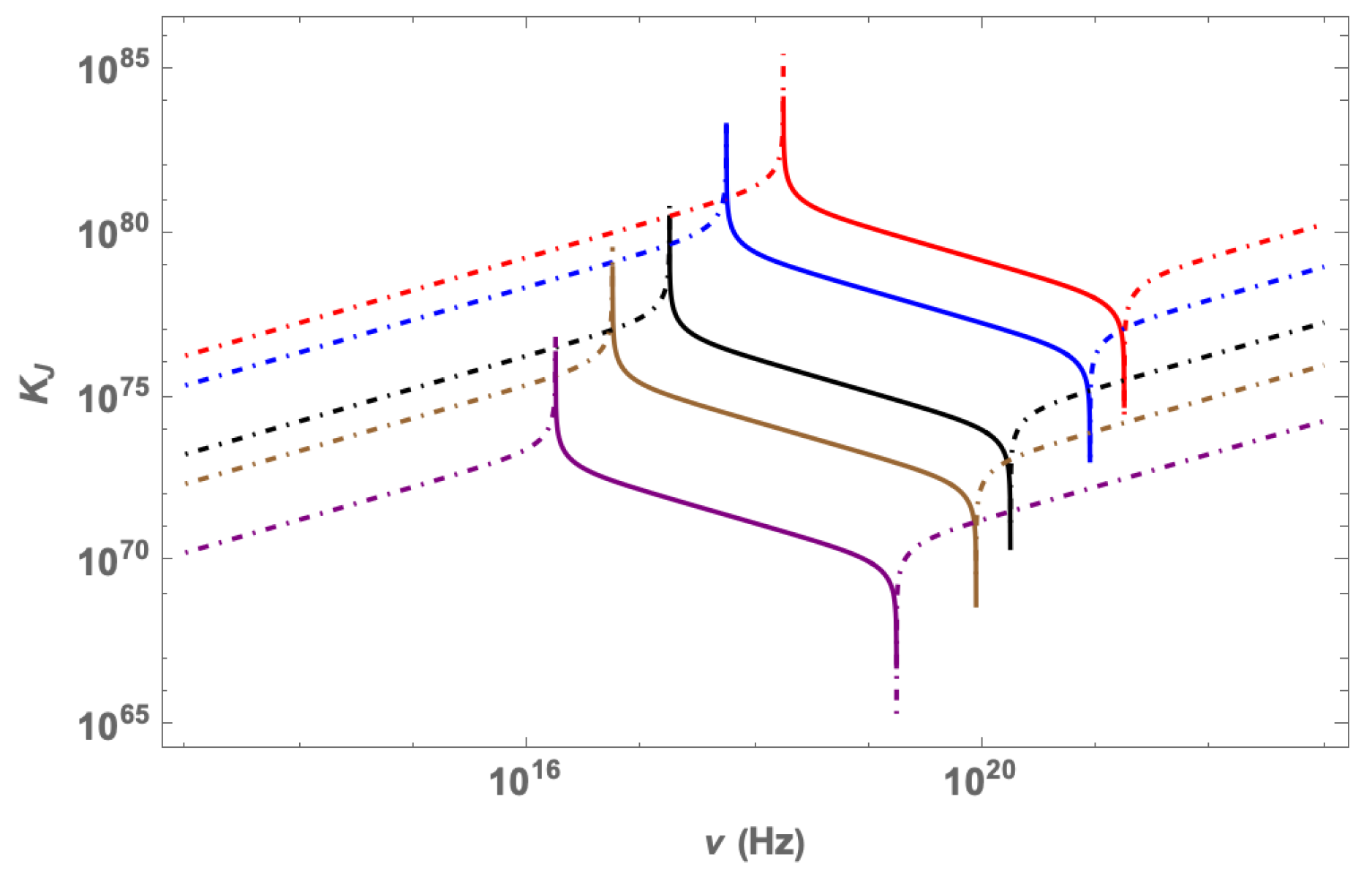
Figure 3.
The polarization index for j=1 (X-mode) is shown by dashed curves and j=2 (O-mode) is shown by the solid curves vs photon frequency is generated using Equation (54) by including finite temperature effect in dielectric tensor.
Figure 3.
The polarization index for j=1 (X-mode) is shown by dashed curves and j=2 (O-mode) is shown by the solid curves vs photon frequency is generated using Equation (54) by including finite temperature effect in dielectric tensor.
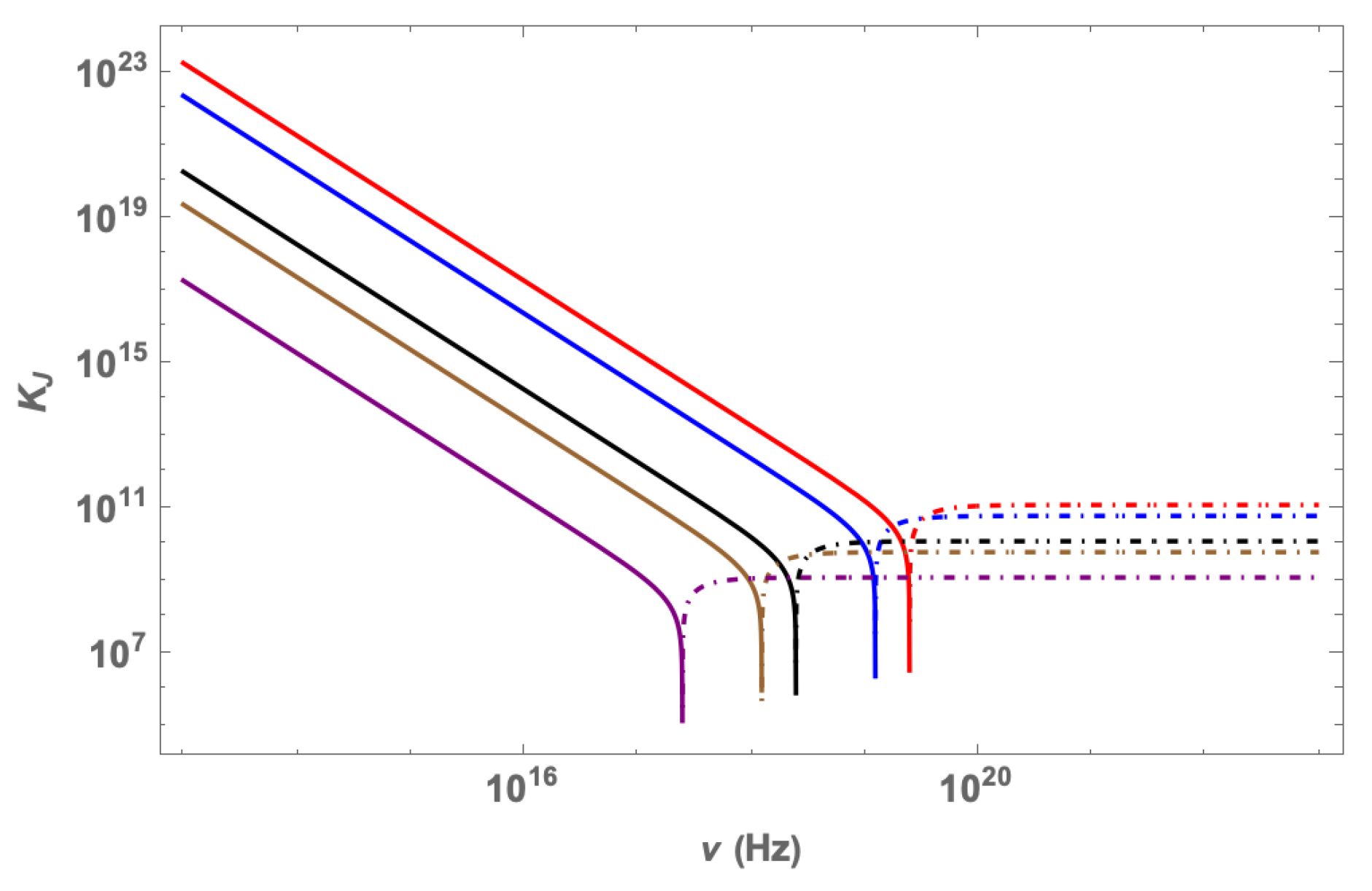
Figure 4.
The variation of electron scattering opacity plotted using Equation (35) against photon frequency at G. The index j=1 is for the X- and j=2 is for the O- mode photon propagation in cold plasma approximation.
Figure 4.
The variation of electron scattering opacity plotted using Equation (35) against photon frequency at G. The index j=1 is for the X- and j=2 is for the O- mode photon propagation in cold plasma approximation.
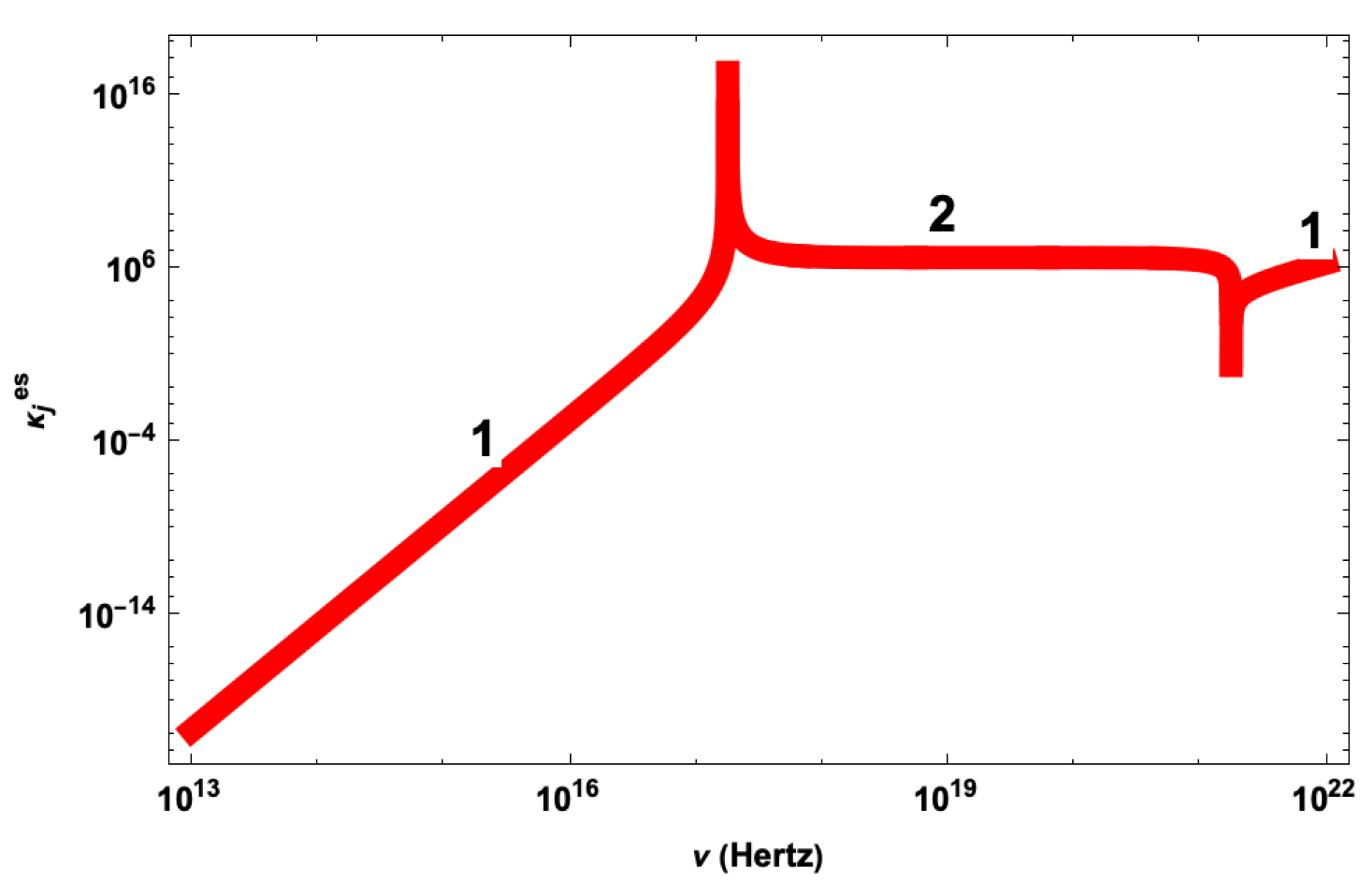
Figure 5.
The variation of electron scattering opacity plotted using Equation (35) against photon frequency at two different strengths of magnetic field (a) G and (b) G. The dashed black and solid red curves are representing the O- and X-mode photon propagation in finite temperature e-i plasma, respectively.
Figure 5.
The variation of electron scattering opacity plotted using Equation (35) against photon frequency at two different strengths of magnetic field (a) G and (b) G. The dashed black and solid red curves are representing the O- and X-mode photon propagation in finite temperature e-i plasma, respectively.
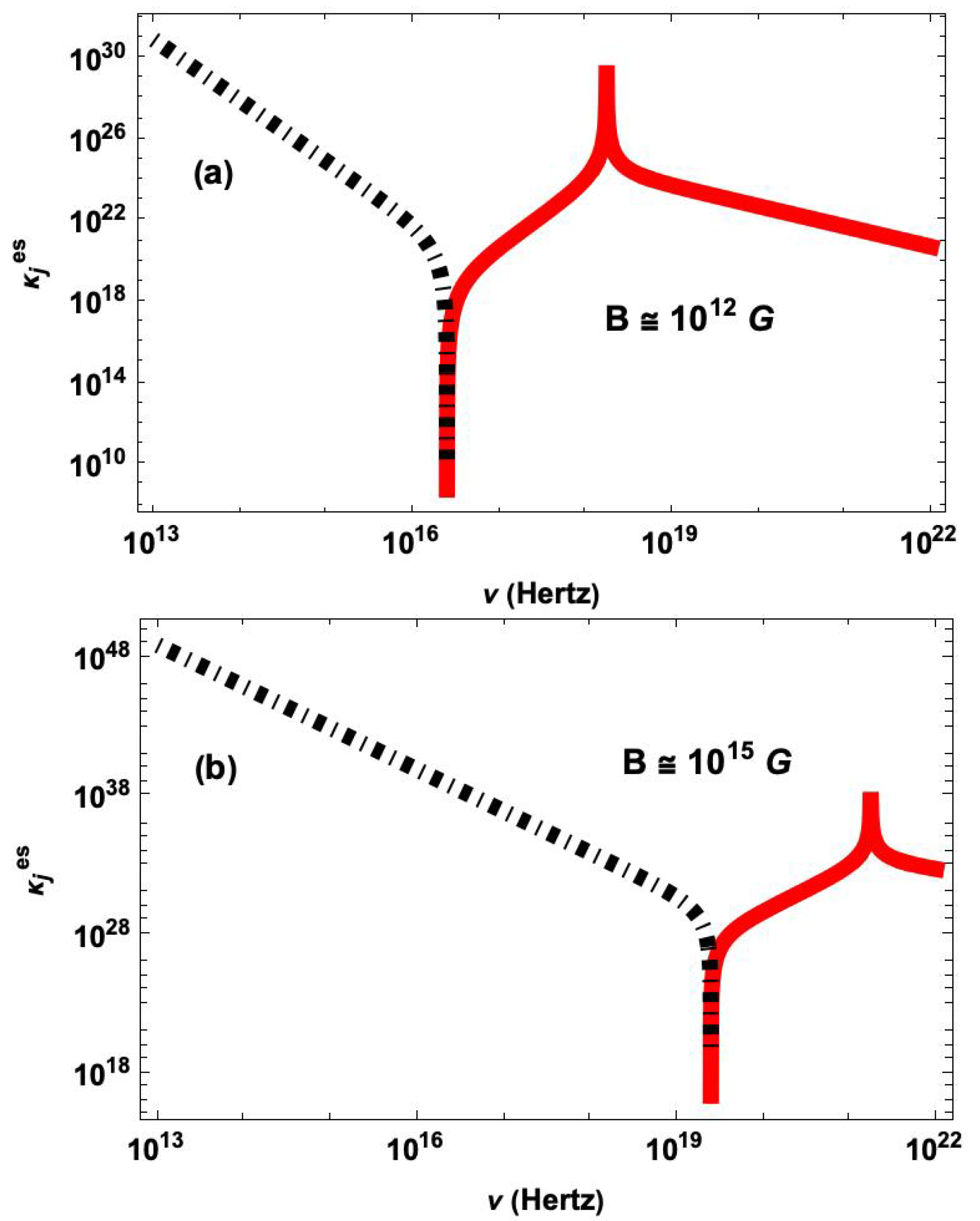
Figure 6.
The variation of free-free (Bremsstrahlung) opacity plotted using Equation (44) against photon frequency at G. The index j=1 is for the X- and j=2 is for the O- mode photon propagation in cold plasma approximation.
Figure 6.
The variation of free-free (Bremsstrahlung) opacity plotted using Equation (44) against photon frequency at G. The index j=1 is for the X- and j=2 is for the O- mode photon propagation in cold plasma approximation.
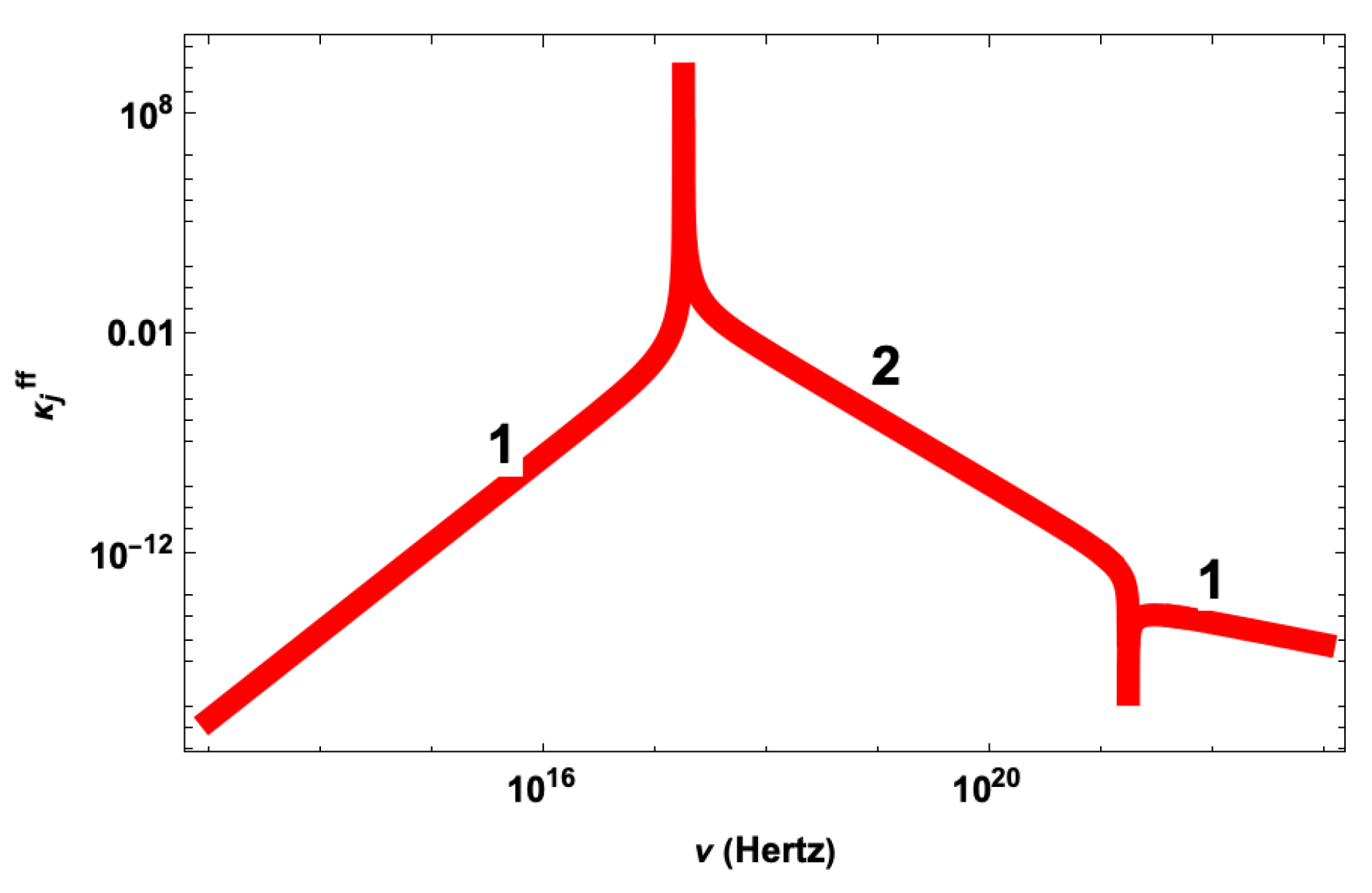
Figure 7.
The variation of free-free (Bremsstrahlung) opacity using Equation (35) against photon frequency at two different strengths of magnetic field (a) G and (b) G. The dashed black and solid red curves are representing the O- and X-mode photon propagation in finite temperature e-i plasma, respectively.
Figure 7.
The variation of free-free (Bremsstrahlung) opacity using Equation (35) against photon frequency at two different strengths of magnetic field (a) G and (b) G. The dashed black and solid red curves are representing the O- and X-mode photon propagation in finite temperature e-i plasma, respectively.
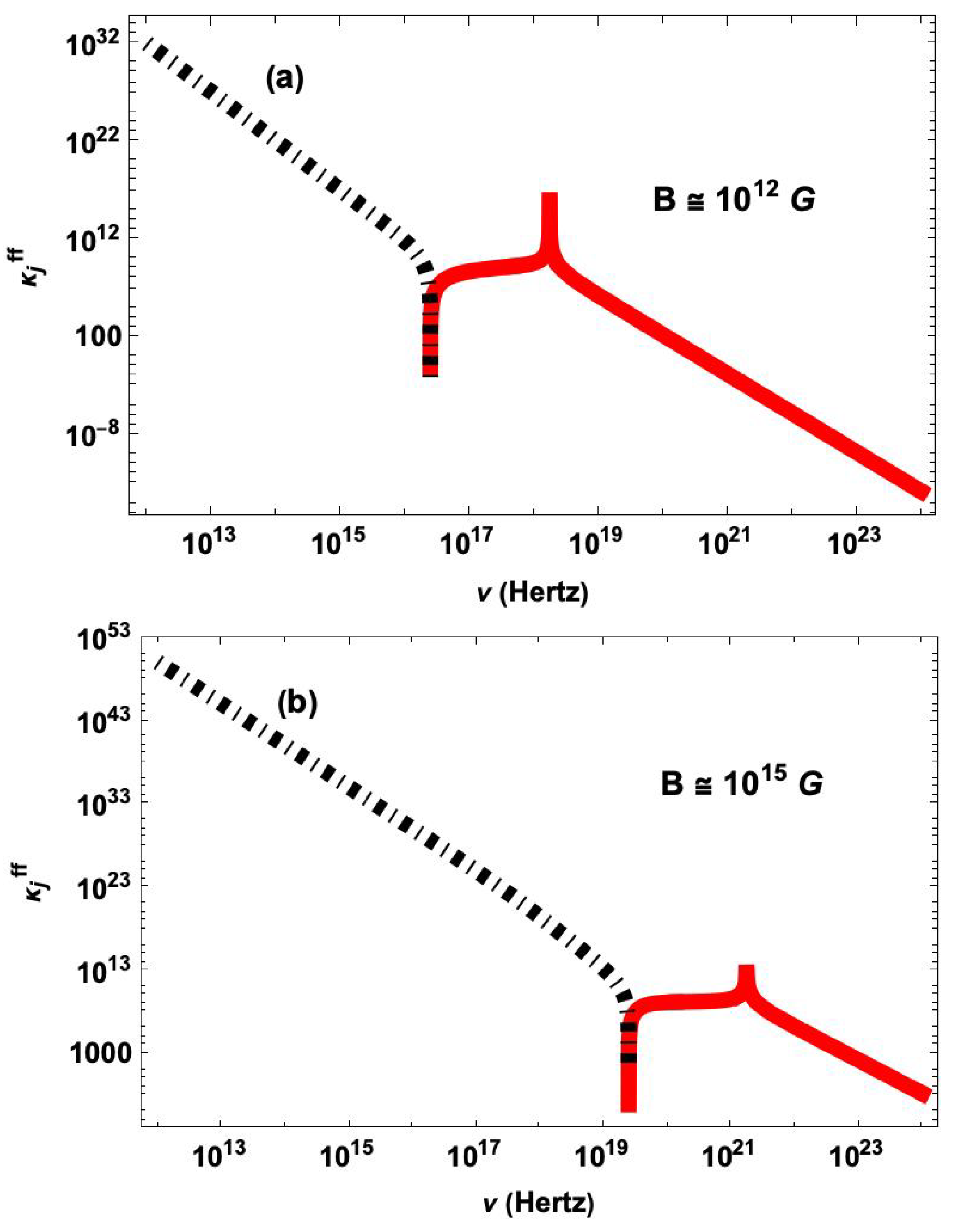
Figure 8.
The modified black-body spectrum at blue, black and red curves with G, and the number density cm−3 is demonstrated. The solid curves represent plotted from Equation (51) and dashed curves is for plotted from Equation (53) of theoretically predicted spectra from the magnetar atmospheres in cold plasma approximation.
Figure 8.
The modified black-body spectrum at blue, black and red curves with G, and the number density cm−3 is demonstrated. The solid curves represent plotted from Equation (51) and dashed curves is for plotted from Equation (53) of theoretically predicted spectra from the magnetar atmospheres in cold plasma approximation.
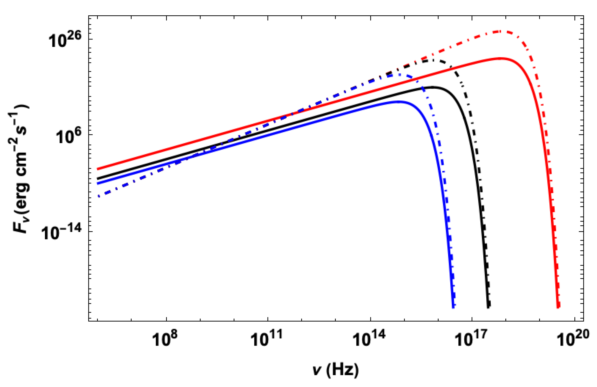
Figure 9.
The emergent modified black-body flux at blue, black and red curves with G, and the number density cm−3 is demonstrated. The solid curves represent plotted from Equation (51) and dashed curves is for plotted from Equation (53) of O-mode photons in finite temperature plasma consideration.
Figure 9.
The emergent modified black-body flux at blue, black and red curves with G, and the number density cm−3 is demonstrated. The solid curves represent plotted from Equation (51) and dashed curves is for plotted from Equation (53) of O-mode photons in finite temperature plasma consideration.
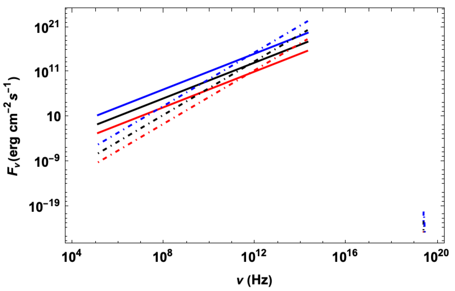
Figure 10.
The emergent modified black-body flux at blue, black and red curves with G, and the number density cm−3 is demonstrated. The solid curves represent plotted from Equation (51) and dashed curves is for plotted from Equation (53) of X-mode photons in finite temperature plasma consideration.
Figure 10.
The emergent modified black-body flux at blue, black and red curves with G, and the number density cm−3 is demonstrated. The solid curves represent plotted from Equation (51) and dashed curves is for plotted from Equation (53) of X-mode photons in finite temperature plasma consideration.
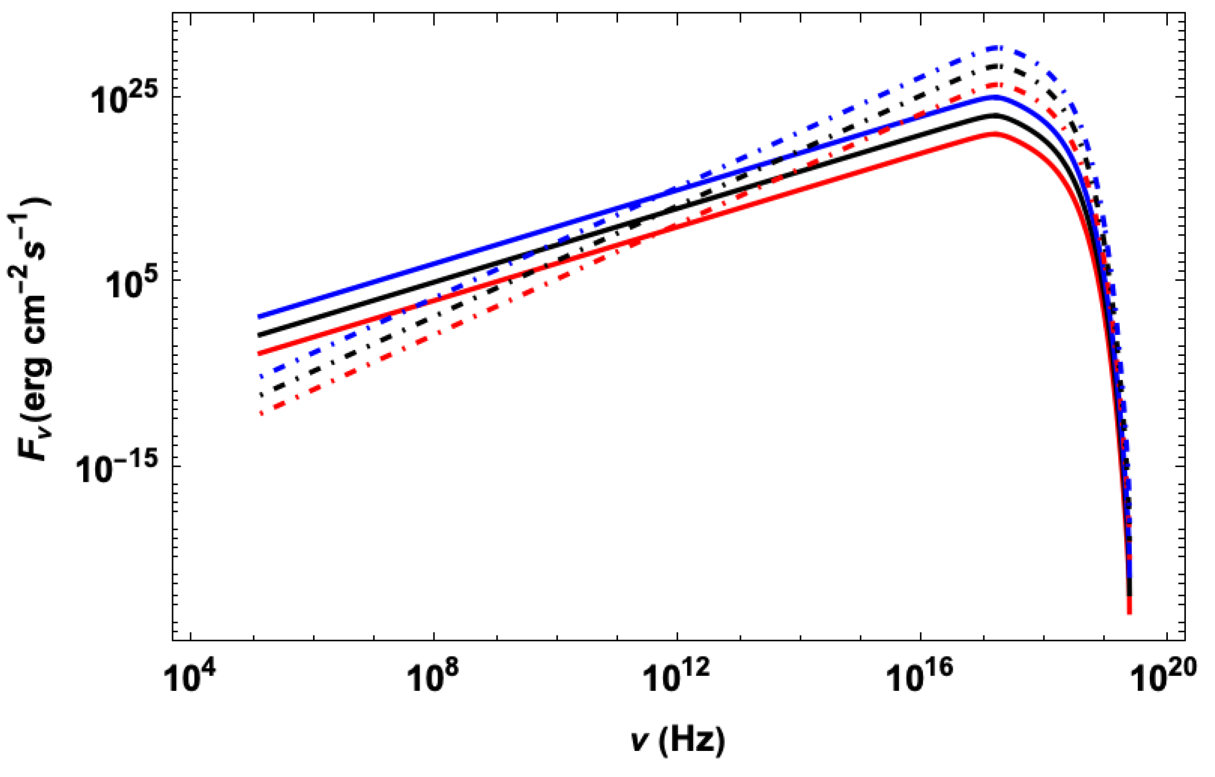

Table 1.
Summary of theoretically predicted flux for particular plasma mode.
| Plasma Mode | Low Frequency | Peak | High Frequency | Polarization Sensitivity |
|---|---|---|---|---|
| Cold Plasma X-mode | RJ IC dominant | Fixed | W-tail | – |
| Cold Plasma O-mode | RJ | Fixed | Steep | – |
| Thermal Plasma X-mode | RJ | Sharp high | Extended tail | Compton shift |
| Thermal Plasma O-mode | Enhanced flux | Higher | Cutoff | Deviated |
Disclaimer/Publisher’s Note: The statements, opinions and data contained in all publications are solely those of the individual author(s) and contributor(s) and not of MDPI and/or the editor(s). MDPI and/or the editor(s) disclaim responsibility for any injury to people or property resulting from any ideas, methods, instructions or products referred to in the content. |
© 2026 by the authors. Licensee MDPI, Basel, Switzerland. This article is an open access article distributed under the terms and conditions of the Creative Commons Attribution (CC BY) license (http://creativecommons.org/licenses/by/4.0/).
Copyright: This open access article is published under a Creative Commons CC BY 4.0 license, which permit the free download, distribution, and reuse, provided that the author and preprint are cited in any reuse.