

Submitted:
20 August 2026
Posted:
24 August 2026
You are already at the latest version
Abstract
The unsteady compressible laminar boundary layer is the natural setting in which the earliest, pre-transitional history of a high-speed viscous flow is written, yet almost no exact solutions of the two-dimensional unsteady compressible boundary-layer equations are known. We extend a recently proposed incompressible similarity transformation [B. H. Sun, Phys. Fluids 36, 083616 (2024)] to compressible flow. Building on the unsteady Howarth--Dorodnitsyn reduction introduced by Stewartson [Q. J. Mech. Appl. Math. 4, 182 (1951), Section 7], and combining it with an undetermined boundary-layer thickness \(\delta(x)\) and a diffusion time \(\tau=C\nu_r t/\delta^{2}\), we show that the compressible mass, momentum and energy equations collapse onto a pair of partial differential equations in two variables (\(\eta\),\(\tau\)) whose coefficients are independent of the streamwise coordinate. Remarkably, the compressible momentum equation differs from its incompressible counterpart only through the replacement 1\(\rightarrow\Theta\)g, where \(g\) is the reduced total enthalpy and \(\Theta=1+\tfrac{1}{2}(\gamma-1)M_e^{2}\). Three applications are developed. (i) The steady limit of the system is shown to be exactly the compressible Falkner--Skan--Dorodnitsyn system, which we solve numerically as a validation. (ii) For the impulsively started semi-infinite plate we obtain two exact solutions of the momentum equation of distinct similarity type---one in Kummer functions, one diffusive---and, at Pr=1, a closed-form Crocco integral for the temperature; for arbitrary Prandtl number the energy equation is integrated in quadrature and yields the closed-form adiabatic recovery factor \(r=(4/\pi)\sqrt{Pr/(2-Pr)}\arctan\sqrt{(2-Pr)/Pr}\), which differs from the classical steady value \(\sqrt{Pr}\). (iii) For m ≠ 0 we solve the unsteady system globally in a Williams--Rhyne chart, in which both ends are characteristic, and show that the transformed wall shear is Mach independent for all time when \(m=0\) but not otherwise, and that the recovery factor migrates continuously from the unsteady closed form to \(\sqrt{Pr}\). Throughout, the sense in which the solutions are exact---exact under the Chapman--Rubesin and constant-Prandtl-number assumptions, in the same sense as the classical steady results---is stated explicitly, and the transformation is validated against the Blasius, Falkner--Skan, Crocco and compressible-Rayleigh results of the classical literature, including the induced outflow \(v_\infty=(\gamma-1)M_w^{2}\sqrt{C\nu_r/2\pi t}\).
Keywords:
unsteady compressible laminar boundary layer
; diffusion-time similarity transformation
; Howarth–Dorodnitsyn reduction
; Falkner–Skan–Dorodnitsyn system
; adiabatic recovery factor
1. Introduction
Since Prandtl’s 1904 boundary-layer concept[1] and the Blasius solution [2], the search for exact solutions of the Navier–Stokes equations has produced a remarkably short list. In his surveys Wang [4,5] counts fewer than 150 genuinely distinct exact solutions after nearly two centuries, most of them steady, and very few of them belonging to boundary-layer flows. For the two-dimensional unsteady boundary layer the situation was, until recently, worse still: since Stokes[6] and Rayleigh[7] posed the impulsive plate problems, only asymptotic and numerical treatments were available [8,9,10,11,12,13,14], and Stewartson’s conjecture[8] that a singularity must be traversed on the way from the Rayleigh solution to the Blasius solution remained open. Sun[15] recently proposed a similarity transformation that reduces the two-dimensional unsteady incompressible boundary-layer equations to a single partial differential equation in two variables whose coefficients do not depend on the streamwise coordinate, and used it to construct closed-form solutions in terms of Kummer functions.
All of this work is incompressible. Yet the flows in which unsteady laminar boundary layers matter most—impulsively started high-speed flows, shock-tube starting flows, hypersonic vehicle transients, and the receptivity phase of high-speed transition[18,19,20]—are strongly compressible. In compressible flow the density is an active variable: it couples the momentum equation to the energy equation through the equation of state, the viscosity varies by an order of magnitude across the layer, and viscous dissipation generates a temperature field that is itself a diagnostic of the coherent structure of the flow. The classical steady compressible boundary layer is understood through the Howarth–Dorodnitsyn [21,22] and Illingworth–Stewartson [23,24] transformations, the Chapman–Rubesin viscosity law[25], the Crocco energy integral [26,27], and the compressible Falkner–Skan–Dorodnitsyn system[24,29,30]. What is missing is an unsteady analogue: a transformation that removes the streamwise coordinate from the unsteady compressible problem, that reduces to the classical steady results in the appropriate limit, and that is explicit enough to expose the analytical building blocks of the solution.
The purpose of this paper is to construct that transformation and to work out its consequences. Our starting point is the observation that the Howarth–Dorodnitsyn variable can be generalised to unsteady flow provided the transformed normal velocity is defined to include the time derivative of the Dorodnitsyn variable itself; with that definition the transformed continuity equation becomes exactly the incompressible one, so that a transformed stream function exists even though the physical flow has . On top of this we apply Sun’s two-fold similarity ansatz: an undetermined thickness used as the normal length scale, and the associated diffusion time used as the time scale. The result (Section 3) is the pair of equations
in which a, b, c are the constants of the incompressible theory and the only new ingredients are the reduced total enthalpy g, the compressibility parameter and the dissipation parameter E. Setting , recovers Sun’s equation exactly.
Two things should be said at the outset about what is and is not new here. The unsteady Dorodnitsyn reduction just described is not ours: it is Section 7 of Stewartson’s 1951 paper[8], whose Eqs. (7.9)–(7.19) contain the transformed normal velocity, the transformed momentum and energy equations, and—under , and an insulated wall—the Crocco integral, the velocity field , the mapping back to physical coordinates and the induced outflow. Everything in Secs. Section 5.4 and Section 5.7 below is his, and is attributed to him there. What this paper adds is what can be built on that reduction once Sun’s similarity ansatz is layered on top: the reduction to with x-independent coefficients for the whole class , whereas Ref. [8] treats only U constant; the pressure-gradient coupling , which vanishes identically in his case and which is what makes the momentum and enthalpy equations interact; arbitrary Prandtl number, arbitrary wall thermal condition and a general Chapman–Rubesin parameter, in place of his , insulated wall and ; the Kummer branch, which lives in the region where he states that the solution is not known; and the global solution of the unsteady problem with pressure gradient in Section 6. A second point of placement: the diffusive branch of Section 5, although it reproduces Stewartson’s velocity field, is shown here to belong to the same two-parameter similarity family as the Kummer branch, so that the two are reductions of one equation rather than solutions of unrelated problems.
The paper is organised as follows. Section 2 formulates the two-dimensional unsteady compressible boundary layer and derives the generalised unsteady Dorodnitsyn transformation. Section 3 introduces the similarity transformation, derives the master system, and determines the class of external velocity distributions for which the coefficients are constants. Section 4 shows that the steady limit of the master system is the compressible Falkner–Skan–Dorodnitsyn system and validates the formulation numerically. Section 5 treats the impulsively started semi-infinite plate: two exact solutions of the momentum equation of distinct similarity type, the Crocco integral at , the quadrature solution and closed-form recovery factor for general , and the wall shear and heat transfer. Section 6 solves the unsteady system for , where the compressibility coupling is active. Section 7 concludes. Appendices collect the Kummer functions, the auxiliary functions of the closed-form solution, the proof of Lemma 1, and the derivation of the recovery factor.
2. The Unsteady Compressible Boundary Layer
2.1. Governing Equations
A thin plate is immersed at zero incidence in a stream of a perfect gas (Figure 1). The origin is at the leading edge, x is measured downstream and y normal to the wall. Outside the layer the flow is inviscid and steady with velocity , temperature , density and Mach number . With the dynamic viscosity, k the thermal conductivity, the specific heat at constant pressure and the static enthalpy, the compressible boundary-layer equations are
closed by and . Because the external flow is steady, and the Bernoulli relation of the outer flow gives
where the second equality uses across the layer. Equation (5) already displays the essential difference from incompressible flow: the pressure gradient acts on a fluid element in proportion to its local temperature, so that the momentum equation cannot be solved without the energy equation.
It is convenient to introduce the total enthalpy
in terms of which () becomes, using (),
Two constitutive simplifications, standard since Refs. [25] and [26], are adopted throughout:
where are constant reference values and C is the Chapman–Rubesin parameter. Equation (8) is exact for a linear viscosity–temperature law and is an excellent approximation over the range of temperatures encountered in most laminar layers; it is the price paid for analytical progress, and it is the same price paid by the classical steady theory.
2.2. An Unsteady Howarth–Dorodnitsyn Transformation
Define the Dorodnitsyn variable
and map with , . In steady flow (9) is the classical Howarth–Dorodnitsyn variable[21,22]; in unsteady flow depends on t through , and the naive definition of a stream function fails because . The remedy is to absorb into the transformed normal velocity.
Lemma 1
(Stewartson’s unsteady Dorodnitsyn reduction). Let
Then the material derivative and the continuity equation take the incompressible forms
This result is due to Stewartson[8], who obtained it in Section 7 of his 1951 paper (his Eqs. (7.9)–(7.14)); we restate it here because everything below depends on it, and give the short proof in Appendix A for completeness. Stewartson’s route is to introduce two potentials and Y with , and , which is the two-dimensional antisymmetric potential representation of the space–time mass flux; eliminating recovers (10). The consequence is decisive: although the physical flow is compressible and unsteady, the transformed flow is solenoidal in the plane, so a transformed stream function exists with
Applying (11), (5) and (8) to () and (7), and noting that implies with , we obtain the transformed compressible boundary-layer equations
In terms of these read
Equations (15)–() are the compressible counterpart of Eq. (7) of Ref. [15], and are equivalent to Stewartson’s Eqs. (7.15), (7.18) and (7.19)[8]. They differ from the incompressible system in exactly two places: the kinematic viscosity is replaced by the effective viscosity , and the pressure-gradient term carries the factor . Everything that follows exploits this structural near-identity.
3. The Similarity Transformation
3.1. Choice of Scales
The physical problem supplies no characteristic length in x and none in y; the only candidate for a normal scale is the boundary-layer thickness measured in the Dorodnitsyn plane, which is left undetermined at this stage and fixed later by the requirement that the transformed coefficients be constants. The time scale follows from dimensional analysis. The relevant parameters and their dimensions are listed in Table 1. Two dimensions (L, T) and four parameters give, by the Buckingham theorem[16,17], two dimensionless groups,
The group is the ratio of the elapsed time to the time required for vorticity generated at the wall to diffuse across the layer—Stuart’s diffusion time[31], here built on the effective diffusivity appropriate to a compressible layer.
Accordingly we set
and, for the thermal field,
with a constant reference total enthalpy and . Two dimensionless compressibility parameters appear:
where is the velocity scale used in (18). For a flow with an external stream it is natural to take and , whence
For the impulsively started plate of Section 5, where the gas at infinity is at rest, the natural choice is , , giving in (20) but ; both cases are covered by the formulae below.
Since and , the temperature and density follow algebraically from f and g:
the second relation reducing to at constant pressure. In particular, with the stream normalisation (21),
3.2. The Master System
The velocity components are therefore
Substituting (24)–() into (15) and (), and using (22) together with the identity , all explicit dependence on disappears provided the three groups
are constants. The result is the master system of this paper:
Three remarks are in order.
(i) Structure. Equation (31) is Eq. (19) of Ref. [15] with the single replacement in the pressure-gradient bracket; setting , recovers the incompressible equation identically. All of the compressibility of the momentum problem is carried by the product , i.e. by the local static temperature. Equation () has exactly the same differential operator as (31) acting on g instead of , with replacing unity in the diffusive term and a dissipation source proportional to . This parallelism is the structural reason for the Crocco integral found in Section 5.4.
(ii) The class of flows. From (30), , so that
with
exactly as in the incompressible theory. The compressible boundary-layer thickness in the physical plane is recovered from , which is larger than by a factor of order ; this is the classical compressible thickening, and it is displayed quantitatively in Figure 2(c).
(iii) When is Θ a constant? Because the outer flow is steady and adiabatic, is a global constant, so g is well defined for any m. The parameter , however, varies with x unless does not, i.e. unless . Thus:
- for (Secs. Section 4 and Section 6) the reduction is exact in the low-Mach limit and is otherwise a local similarity statement, in which and are frozen at their local values. Local similarity is the standard device of compressible boundary-layer theory [28,29] and its error is of the same order as the other approximations we make.
Table 2 places the present transformation beside its predecessors.
3.3. Boundary Conditions
At a solid wall we require no slip and no penetration; in the transformed variables, for a wall at rest in a stream,
while for a wall moving in its own plane with speed into gas at rest (Section 5)
The thermal condition is either a prescribed wall temperature or a prescribed wall heat flux. Because , the adiabatic condition reads
For a wall at rest the right-hand side vanishes and (37) reduces to the familiar ; for a moving wall it does not, because the wall then does viscous work on the gas. Overlooking this term leads to an unphysical cooling of an adiabatic moving plate, and we shall see in Section 5.5 that retaining it restores the classical recovery temperature at . In all cases .
4. The Steady Limit
Before exploiting the master system it is worth confirming that it contains the classical steady theory. Setting in (31)–() and choosing (a normalisation, since a may be absorbed in ) gives, with ,
subject to , , and either or . From (34) with ,
which is precisely the Falkner–Skan pressure-gradient parameter[3], and (38)–() are the compressible Falkner–Skan–Dorodnitsyn equations of the classical steady theory[24,29,30]. Thus the present unsteady transformation degenerates correctly.
Equations (38)–() were solved with a collocation boundary-value solver on with a tolerance of . Figure 2 and Table 3 summarise the results. Three classical facts are reproduced, and they serve as validation of the whole formulation:
- 1.
- At the term vanishes and (38) collapses to the Blasius equation regardless of and of the thermal boundary condition. We obtain , i.e. in the present normalisation , for every Mach number tested. Compressibility affects the flat-plate skin friction only through the Chapman–Rubesin factor C and through the density weighting of the Dorodnitsyn mapping—the classical result.
- 2.
- At the energy equation is solved exactly by , giving an adiabatic wall temperature , i.e. a recovery factor of unity.
- 3.
- For the computed recovery factor agrees with to better than over (Figure 7(a), open squares).
- 4.
- The unsteady flow with pressure gradient. Solved globally in a Williams–Rhyne chart, in which is not a marching variable because changes sign at Stewartson’s line . The transformed wall shear is Mach independent at every instant when , and strongly Mach dependent otherwise; the recovery factor is a function of time, running from the closed form (61) at the impulsive start to at the steady state, and undershooting both when .
5. The Impulsively Started Semi-Infinite Plate in a Compressible Gas
5.1. Statement and Reduction
A semi-infinite plate lies in a viscous, thermally conducting gas at rest with temperature and density . At the plate is impulsively set in motion in its own plane with constant speed . This is the compressible version of Stokes’ first problem[6] on a semi-infinite plate, and its incompressible version is the problem addressed by Stewartson[8,10], Hall[11], Dennis[12] and Sun[15]. We take , , and define the wall Mach number and the associated stagnation ratio
Here is constant, so and hence . Taking the normalisation gives and, from (33),
Because , the pressure-gradient bracket disappears from (31) and the momentum problem decouples completely from the thermal problem:
This is exactly Eq. (25) of Ref. [15]. We have therefore established a useful equivalence:
For a perfect gas obeying the Chapman–Rubesin law, the velocity field of the unsteady compressible flat-plate boundary layer is obtained from the incompressible one by the substitutions and ; every incompressible solution of (43) lifts to a compressible solution.
The thermal field, in contrast, is genuinely new and is determined by () with , .
5.2. The Sense in Which the Solutions Are Exact
Because the phrase “exact solution of the compressible boundary-layer equations” is easily over-read, we state precisely what is and is not claimed.
The construction rests on four assumptions, of which only the first two are innocuous. (i) The boundary-layer (Prandtl) ordering, so that (1)–() replace the Navier–Stokes equations; the initial pressure transients and compression waves of the exact impulsive problem[36,37,38] are thereby excluded. (ii) A calorically perfect gas. (iii) The Chapman–Rubesin law with C constant. (iv) A constant Prandtl number. Given (i)–(iv), Lemma 1 is an identity, the reduction to (31)–() involves no further approximation when , and the diffusive branch (50) together with the temperature field of Secs. Section 5.4Section 5.5 satisfies the resulting system and all its boundary conditions identically. In that sense the solutions are exact.
This is precisely the sense in which the classical steady compressible results are called exact. The statement that a flat-plate compressible layer at reduces to the Blasius problem, the Crocco integral[26], and the Illingworth–Stewartson transformation[23,24] are all exact consequences of (i)–(iv) and are all invalidated, as exact statements, by a Sutherland viscosity law or a variable . Under Sutherland’s law C varies through the layer and the present solutions become leading-order approximations whose error is ; for air below with a reference temperature evaluated by Eckert’s rule this is a few per cent, and it is the same error already accepted throughout classical compressible boundary-layer theory[29,30]. Recent work on temperature–velocity relations in hypersonic laminar layers[41,42] quantifies the departure from the Chapman–Rubesin/Crocco picture at high enthalpy and should be consulted before applying (61) at hypersonic conditions.
5.3. Two Exact Solutions of Distinct Similarity Type
We use the word branch throughout for a solution of (43) obtained by imposing a particular similarity structure on . The two branches constructed below are not two solutions of a single well-posed problem, in the sense in which the Falkner–Skan equation possesses dual solutions for : they satisfy the same wall conditions but different conditions at infinity, and neither is obtainable from the other by any choice of the constants of integration.
5.3.1. The Kummer Branch
Equation (43) admits the closed-form solution obtained in Ref. [15],
where and are the combinations of Kummer functions of the first and second kind given in Appendix B and are constants of integration. Boundedness of requires ; the no-slip condition and the normalisation then give
numerically , . The wall shear follows from
We have verified by direct symbolic-numeric substitution that (44) satisfies (43) to machine precision (residuals over , ); the auxiliary functions in Appendix B contain a typographical correction to Ref. [15] noted there.
Figure 3 shows f, , and at and the velocity profiles at several . Two properties deserve emphasis. First, the solution satisfies the wall conditions exactly for every . Second, its outer limit is
so the far-field condition is attained only asymptotically, as . This is not a defect of the transformation but a property of this particular branch: it is an accurate representation of the flow in the Rayleigh region , i.e. (Figure 5), and degrades as the Blasius region is approached.
It follows that the Kummer branch is an exact solution of the equation but not of the problem: it satisfies (43) identically and meets the wall conditions for all , but attains the outer condition only as . We describe it throughout as an exact solution of the reduced equation, and do not claim that it solves the impulsive-plate boundary-value problem.
5.3.2. The Diffusive Branch
The master equation (43) possesses a second, hitherto unremarked exact branch which satisfies all of the boundary conditions. Seek solutions of the self-similar diffusive form
the last equality following from (42) and being independent of x. Substituting (48) into (43) and using , , , , , every nonlinear term cancels identically and there remains
Hence
so that
It must be stressed that the vanishing quantity in (51) is the transformed normal velocity V, not the physical one: by (10), , and because dissipative heating changes the density. The physical normal velocity is computed in Section 5.7, where it is shown to reproduce the outflow that is the classical signature of the compressible Rayleigh problem[35,36,37]. Indeed, any f of the form satisfies , which is precisely the transformed statement ; the third condition in (36) is therefore satisfied identically, and (50) gives and exactly. The diffusive branch is thus the compressible Rayleigh solution, and the content of the present derivation is that it belongs to the similarity family (18): the classical Rayleigh solution is a member of the same two-parameter family that contains the Kummer branch. In the physical plane it is not an error function of y, because and y are related through the temperature field; the profile in y is obtained by the quadrature , which is carried out in Figure 8.
5.3.3. Relation between the Branches and Stewartson’s Conjecture
Both branches solve the same equation with the same wall conditions, so they differ in the outer condition and in the initial data. Letting at fixed in (44) gives
with ; Figure 4(a) confirms that the profiles collapse onto this curve. It is a genuinely different self-similar profile from , and the corresponding wall shear coefficients differ,
as shown in Figure 4(b). Since the diffusive branch reproduces the exact solution of the physical Rayleigh problem, we regard it as the physically relevant branch at early times, and the Kummer branch as a second exact solution of the reduced equation whose interest is analytical. Both are regular at (Figure 4(c)), which supports Sun’s conclusion[15] that the passage from the Rayleigh to the Blasius regime, contrary to Stewartson’s conjecture[8], need not traverse a singularity: the value marks the change of sign of the coefficient multiplying in (), i.e. a change of the direction in which information propagates in , not a singularity of the solution.
Figure 4.
The two exact branches compared. (a) The Kummer branch velocity, with its outer residual removed, collapses as onto the limiting profile of Eq. (52) (dotted), which is distinct from the diffusive branch (dashed). (b) Transformed wall shear: both branches decay as but with different coefficients, and . (c) The velocity field of the Kummer branch in the plane; the line , at which changes sign, is regular.
Figure 4.
The two exact branches compared. (a) The Kummer branch velocity, with its outer residual removed, collapses as onto the limiting profile of Eq. (52) (dotted), which is distinct from the diffusive branch (dashed). (b) Transformed wall shear: both branches decay as but with different coefficients, and . (c) The velocity field of the Kummer branch in the plane; the line , at which changes sign, is regular.
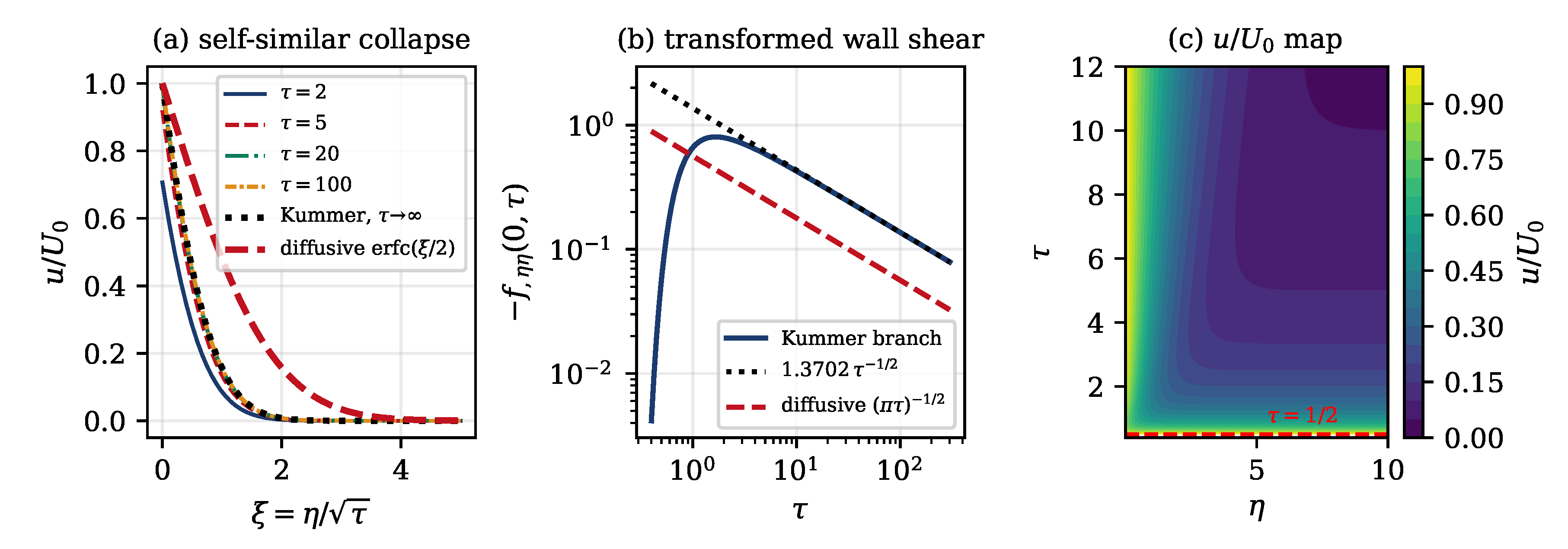
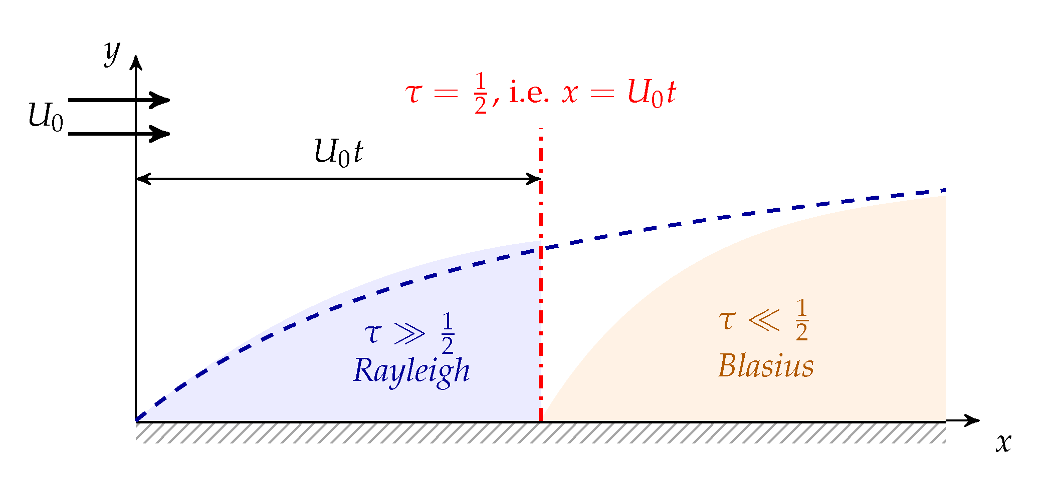
Figure 5.
Regions of the unsteady boundary layer past an impulsively started plate. Near the leading edge is large and the flow is essentially the one-dimensional Rayleigh (Stokes) layer; far downstream is small and the flow has not yet felt the start-up, approaching the Blasius state. The similarity variables (42) span both regions continuously.
Figure 5.
Regions of the unsteady boundary layer past an impulsively started plate. Near the leading edge is large and the flow is essentially the one-dimensional Rayleigh (Stokes) layer; far downstream is small and the flow has not yet felt the start-up, approaching the Blasius state. The similarity variables (42) span both regions continuously.
5.4. The Thermal Field at : a Crocco Integral
With the energy equation () at becomes
which is precisely (43) with g in place of . Hence both and solve it, and so does any linear combination:
This is the unsteady compressible analogue of the Crocco integral[26,27], valid for arbitrary . It is exact whenever ; for the residual is and (55) becomes an approximation.
Applying with gives . For an adiabatic wall the boundary condition (37) with gives , so and, from (22),
The adiabatic wall therefore attains the full stagnation temperature based on the plate speed, a recovery factor of unity, exactly as in the steady theory—but now at every instant, and for the moving-wall configuration in which the wall itself supplies the dissipation. For a prescribed wall temperature ,
a two-parameter family whose linear term measures wall heat transfer and whose quadratic term measures viscous dissipation. Profiles are shown in Figure 6(a),(b) using the diffusive branch .
5.5. Arbitrary Prandtl Number: Quadrature and Recovery Factor
On the diffusive branch the energy equation reduces to an ordinary differential equation. Writing with and substituting into () with , , all terms proportional to cancel and there remains
It is more transparent to work with the static temperature . Using from (49), Eq. (58) collapses to the classical dissipation equation
whose solution is elementary:
For an adiabatic wall , and integrating (60) once more with gives, after interchanging the order of integration and transforming to polar coordinates (Appendix C),
for the recovery factor defined by . For the analytic continuation applies, and . Equation (61) gives , consistent with the Crocco integral, and . It is not equal to : the unsteady Rayleigh layer recovers more than the steady Blasius layer for and less for (Table 4 and Figure 7). For air at , against the Blasius value , a difference of in the recovery excess, which for amounts to about in wall temperature.
Equation (61) is an exact consequence of the assumptions listed in Section 5.2. We have not found it in the literature on the compressible Rayleigh problem[35,36,38,39,40], which is largely confined to small Mach number and to near unity or to special values such as ; but that literature is old and scattered, and we state only that we are unaware of a prior derivation, not that none exists.
5.6. Arbitrary Prandtl Number on the Kummer Branch
Section 5.5 solved the energy equation on the diffusive branch. On the Kummer branch the thermal field has so far been available only at , through the Crocco integral (55). We now close that gap. The route is the group-invariant reduction of the unsteady energy equation, and the key observation is that the cancellation exploited in (58)—“all terms proportional to cancel”—is not an accident of the diffusive branch but an instance of a general mechanism.
5.6.1. The Static-Temperature Form
Write the convective operator of () at , as
so that the energy equation reads .
Lemma 2
(Static-temperature form). Let . Then, whenever ,
Proof.
Equation (63) is the compressible statement that the static temperature obeys a passive-scalar equation with the viscous-dissipation source , the Eckert number of the incompressible theory being replaced by . It is the unsteady, compressible counterpart of the Pohlhausen energy equation, and it is branch-independent: applied to the diffusive branch it reproduces (59) immediately.
5.6.2. Why the Convection Is Blind to the Velocity Field
Lemma 3
(Velocity-blind convection). For any ,
On the diffusive branch one has and hence with . On the Kummer branch (44) one has with
and hence . In either case, if ζ is an invariant of the corresponding generator, or , then contains no reference to f whatever.
Proof.
Lemma 3 explains the cancellation observed in (58) and supplies its analogue for the Kummer branch. The invariant of X is
and (46) shows that the Kummer velocity field is itself group-invariant up to the outer drift:
with , , , and
and .
5.6.3. Exact Reduction and Closed-Form Thermal Field
Theorem 1.
On the Kummer branch, satisfies (63) for arbitrary and E if and only if
Proof.
Equation (69) is linear with integrating factor . Imposing and a wall value gives the closed form
with
Since , dissipation alters the interior profile but not the boundary values. The wall gradient is
For the temperature is simply a complementary error function of the group invariant, , which as becomes in the Dorodnitsyn variable; the physical-plane profile follows, as everywhere in this paper, from the quadrature . Setting gives the adiabatic wall temperature , i.e. the recovery factor
We have verified by substitution in 25-digit arithmetic that , with from (70), satisfies () with residuals below over , , , .
5.6.4. Comparison of the Branches, and a Caution
Table 5 places (74) beside the diffusive value (61) and the steady . Two features deserve comment, and the second is a caveat rather than a result.
First, the two branches recover differently at every , and the Kummer branch recovers more. This is consistent with its velocity field: the Kummer wall shear coefficient exceeds the diffusive one by the factor , so the dissipation integral that feeds the wall temperature is correspondingly larger. In the limits as and as , so the Kummer branch shares the scaling of the steady layer at small but saturates logarithmically at large , whereas (61) tends to .
Second, at the Kummer branch carries two exact adiabatic solutions that satisfy the same asymptotic conditions: the Crocco integral (55), which gives , and the group-invariant solution (70), which gives . They are genuinely distinct: , so the Crocco field is not group-invariant. The origin of the ambiguity is the same degeneracy that limits the Kummer branch itself. The coefficient of vanishes as , so is a degenerate characteristic on which no Cauchy data are prescribed; and the wall corresponds to , not to , so a condition imposed at —isothermal or adiabatic—is met only as , exactly as the velocity conditions are. Within the group-invariant class (70) is unique, which is the natural similarity-theoretic statement; the spread between 1 and is an honest measure of the residual indeterminacy of this branch. The diffusive branch is free of this difficulty—it satisfies all of its boundary conditions exactly at every —and (61) therefore remains our physical prediction for the compressible Rayleigh layer. Equation (74) is offered as the thermal completion of the Kummer branch, in the same spirit in which Section 5 offers the branch itself: an exact solution of the reduced equation whose interest is analytical.
5.6.5. Remark: There Is No Systematic Correction
It is natural to try to relax the asymptotic character of the wall conditions by writing . This does not work in the expected way. Using Lemma 3 and (67),
so that the term contributes to the leading balance and the hierarchy closes algebraically rather than differentially:
and similarly divided by . The corrections are therefore proportional to the residual of (69) itself, and each successive term carries another factor , which diverges in the outer region. The choice —that is, Theorem 1 —is the only consistent truncation, and relaxing the restriction requires a different device, presumably a -dependent shift of the invariant rather than a series in .
5.7. The Induced Outflow, and Comparison with Classical Results
The compressible Rayleigh problem differs from its incompressible counterpart in one qualitative respect, emphasised by Howarth[35], Van Dyke[36] and Stewartson[8,37]: viscous dissipation heats the gas, the gas expands, and a normal velocity directed away from the plate is induced even though the plate moves purely in its own plane. Our formulation must reproduce this, and it provides a quantitative check on the transformation that is independent of the incompressible limit.
On the diffusive branch the flow is independent of x, so , and ; hence . Writing and with and , differentiation at fixed y gives
which vanishes identically when , as it must. At the outer edge and (77) tends to the finite limit
an outflow, as anticipated. At with an adiabatic wall the Crocco integral (56) gives , and since exactly,
The outflow decays as , grows as the square of the wall Mach number, and is independent of x. Both the scaling and the dependence agree with the small-Mach-number analyses of Van Dyke[36] and Hanin[38], which were obtained by linearising the full Navier–Stokes equations rather than by the boundary-layer approximation used here; (79) extends the result to arbitrary within the Chapman–Rubesin model. We note that those analyses also capture the initial pressure and temperature transients and the compression waves discussed by Stewartson[37], which lie outside the boundary-layer approximation and are therefore absent from (79).
5.8. Validation against Established Results
Table 6 collects the quantitative checks available to us. Each is a case in which the present formulation must reproduce an independently established result, and each tests a different ingredient: the momentum reduction, the pressure-gradient term, the Crocco closure, the energy equation at , and the density coupling that produces the outflow.
Two entries deserve comment. The steady recovery factor at agrees with to ; the residual is not numerical error but the known departure of the exact Falkner–Skan–Dorodnitsyn result from the approximation, and its sign and magnitude match the tabulations of Ref. [30]. The outflow entry is an exact coefficient agreement, not merely a scaling one: setting () in (79) reproduces Eq. (7.25) of Ref. [8] term for term, including the factor . The agreement is a non-trivial check, since it tests the density coupling, the Crocco closure and the inverse mapping (82) simultaneously. The small-Mach Navier–Stokes analyses of Refs. [36,38] agree in exponent and in the dependence but carry additional terms, from the initial pressure transient, that lie outside the boundary-layer approximation.
We have not been able to compare the unsteady recovery factor (61) at against an independent calculation, since we know of none; it is checked here only against numerical quadrature of (59) (Table 4), which shares its assumptions. This is the weakest link in the validation chain and we flag it as such.
5.9. Wall Shear, Heat Transfer and the Physical Plane
On the diffusive branch the wall quantities follow in closed form. With and ,
independent of x, as it must be in the Rayleigh region, and depending on compressibility only through C. The wall heat flux follows from (60), which gives the Newtonian form and hence
with r from (61). The Reynolds analogy factor is , again differing from the steady flat-plate value .
Finally, the solution must be mapped back to the physical plane. Inverting (9),
which is evaluated in Figure 8. The heated gas near a high-speed plate is light, so a fixed amount of mass occupies a much greater physical thickness: at the layer is roughly three times thicker than the incompressible layer at the same time, and the density at the wall falls to about a quarter of its free-stream value. This is the familiar mechanism by which compressibility destabilises and thickens high-speed boundary layers.
6. The Unsteady Flow with Pressure Gradient
Section 4 and Section 5 exercise the master system only where its distinctive term is inactive: the steady limit is classical, and the flat plate has , so the coupling vanishes identically. We now solve (31)–() for , which is where the momentum and enthalpy equations genuinely interact.
6.1. Why Is Not a Marching Variable
Collecting the -derivatives in (31),
so the coefficient of vanishes where . At the outer edge this is , which for is : precisely Stewartson’s line . Beyond it the coefficient is negative over part of the layer, the problem is backward-parabolic in there, and no forward march in can succeed. We confirmed this numerically: an implicit march from the Rayleigh start diverges near irrespective of step size. This is not a defect of the transformation but the analytical content of Stewartson’s essential singularity, expressed as a change of characteristic direction.
6.2. A Uniformly Valid Chart
Introduce, following the device of Williams and Rhyne[46],
so that and, at small s, independently of x. Substituting (84) into (31)–(), the terms in cancel identically and there remains
where acts on and G as second-order operators,
The two ends are characteristic, since , and each carries its own ordinary differential equation:
the Rayleigh start and, after the substitutions , , exactly the Falkner–Skan–Dorodnitsyn system (38) of Section 4. The chart therefore spans the entire history from impulsive start to steady state, and no condition may be imposed at either end: the solution is determined by the equations alone.
Because the sign change survives (84)—it is now confined to the factor , which vanishes at both ends—we do not march. We solve (85)–() globally on the rectangle , by Newton–Krylov relaxation, with central differences in s and second-order differences in N, imposing only , , and the wall thermal condition.
6.3. Results
Table 7 and Figure 9 summarise the solution. The computed limit reproduces to four figures for every , and the limit reproduces the independently computed steady wall shear of Section 4 to better than ; since the two calculations share no code path, this is a genuine check on both. Three results follow.
(i) The coupling is inactive only at . For the transformed wall shear is Mach independent at every s, not merely in the steady limit—the curves for , 2 and 4 collapse to plotting accuracy (Figure 9(c)). This extends the classical steady statement to the whole unsteady history. For the same curves separate widely, , and at , 2, 4: it is the product , not b alone, that sets the effective pressure gradient, and at compressibility increases the steady wall shear by over its incompressible value at the same .
(ii) The recovery factor is a function of time. At it falls monotonically from at —the closed form (61), which gives —to at , against . The two limiting results of this paper are therefore the two ends of a single curve, and the transition occupies , that is . A short-duration facility whose test time falls inside this window recovers neither value.
(iii) Pressure gradient depresses the recovery factor below both limits. For the curve undershoots , reaching at –, before settling. The adiabatic wall of an accelerating compressible layer is thus cooler, relative to its own stagnation temperature, than either classical limit would suggest.
The solver converges for . The single value , at which vanishes and the -derivative structure degenerates, required continuation and is not reported; the steady limit at is given in Section 4.
7. Conclusions
We have extended the unsteady incompressible similarity transformation of Sun[15] to the two-dimensional compressible laminar boundary layer. The principal results are the following.
- 1.
- 2.
- A master system. With , and , the compressible equations reduce to the pair (31)–(), whose coefficients a, b, c are independent of x for the class with , . The compressible momentum equation differs from the incompressible one only by the replacement . All the compressibility of the momentum problem is carried by the local static temperature.
- 3.
- Correct degeneration. The steady limit is exactly the compressible Falkner–Skan–Dorodnitsyn system, and numerical solution recovers independent of Mach number at , at , and —all classical.
- 4.
- Two exact solutions for the impulsively started plate. Besides Sun’s Kummer-function branch we found a diffusive branch with , which reduces (43) exactly to and satisfies all boundary conditions, including . It is the compressible Rayleigh solution, and it is a member of the same similarity family. The two branches have wall-shear coefficients and . Both are regular at , supporting Sun’s conclusion that the Rayleigh–Blasius transition need not be singular.
- 5.
- An unsteady Crocco integral and a closed-form recovery factor. For the enthalpy equation at is solved exactly by for all . For arbitrary the energy equation on the diffusive branch integrates in quadrature and yieldswhich equals unity at but is otherwise not: for air, against . The associated Reynolds analogy factor is rather than . Obtaining this required the observation that the adiabatic condition at a moving wall is , not .
Several limitations should be stated plainly. The Chapman–Rubesin approximation and constant are essential to the reduction; relaxing them destroys the exact decoupling, though the transformation survives as a leading-order approximation. For the parameter varies with x and the reduction is a local-similarity statement. The Kummer branch solves the reduced equation but meets the outer condition only as . And nothing here addresses stability: whether the profiles exhibited are selected and persist is a separate question, and the natural next step is a linear stability analysis of the branches of Section 5 against the Mack modes[18] of high-speed boundary layers. Extending the reduction to a pressure-gradient flow with , where the coupling is active and the momentum and energy equations no longer separate, is the obvious next analytical step.
Author Contributions: Bo Hua Sun
: Conceptualization, Methodology, Formulations, Formal analysis, Funding acquisition, Investigation, Writing- Original draft preparation, Writing- Reviewing and Editing and all relevant works.
Data Availability Statement
The data supporting the findings of this study are available from the corresponding author upon reasonable request.
Acknowledgments
My investigations into the boundary layers started from my tenure as a professor at the Cape Peninsula University of Technology (CPUT), South Africa. I am profoundly grateful to CPUT for granting me complete academic autonomy to advance this research agenda. This vital institutional support laid the foundation for the principal conclusions presented in this manuscript. I also extend my deepest gratitude to former Vice-Chancellor (now Chancellor) Prof. Brian Figaji, and former Deputy Vice-Chancellors Prof. J. A. Tromp and Prof. Anthony Staak, for their generous support and endorsement. Further academic support was provided by Xi’an University of Architecture and Technology (XAUAT) and the Beijing Institute of Nanoenergy and Nanosystems (BINN), Chinese Academy of Sciences. I sincerely thank former XAUAT President Prof. Xiao-Jun Liu and current President Prof. Xiang-Mo Zhao, along with BINN Founding Director Prof. Zhong Lin Wang, for their unwavering encouragement and invaluable resource support throughout this study.
Conflicts of Interest
The authors declare that there are no competing financial interests.
Appendix A. Proof of Lemma 1
Under the map defined by , and (9), the chain rule gives
where and are evaluated at fixed and y respectively. Hence the material derivative is
which is the first assertion. For the second, differentiate (10) with respect to using and , :
At the same time, from the second relation in (A1),
Two remarks. First, the physical normal velocity is recovered from V by inverting (10), , which is Eq. (). Second, at a solid impermeable wall we have , and , so : the transformed wall is also impermeable, and the transformed boundary conditions are the familiar ones.
Appendix B. Kummer Functions and the Auxiliary Functions of the Kummer Branch
Appendix B.1. Definitions
Appendix B.2. The Functions h 11 and h 12
With the similarity argument
the auxiliary functions entering (44) are
and , are obtained from (A10)–() by replacing with ; because does not decay as , these are the unbounded solutions and are discarded. Differentiating () once more and using the contiguous relation gives the compact form (46) for .
Correction. In Eq. (B1) of Ref. [15] the argument (A9) is printed with in the denominator. The exponent must be 3, as in (A9); with the function (44) does not satisfy (43), whereas with (A9) we verified the residual of (43) to be over , , and the internal consistency checks and , to the same accuracy. We note this because the dimensional argument X must scale as for large at fixed , which (A9) does and does not; this is what makes the limit (52) exist.
Appendix C. Derivation of the Closed-Form Recovery Factor
We integrate (59) with (adiabatic wall) and . The first integral is (60) with the bracket reduced to its second term. Integrating once more from 0 to ∞,
Substituting and , the exponent becomes , the Jacobian is , and the wedge maps to the sector with
In polar coordinates , so
Since and, by definition, , we obtain (61). The expression is real and increasing for ; at the sector angle and the prefactor combine to the finite limit , and for the substitution replaces the circular sector by a hyperbolic one and arctan by artanh, giving the continuation quoted in the text. ▪
References
- Prandtl, L. Über Flüssigkeitsbewegung bei sehr kleiner Reibung. Verhandlungen des III. Internationalen Mathematiker-Kongresses (Teubner, Leipzig, 1904; pp. 484–491. [Google Scholar]
- Blasius, H. Grenzschichten in Flüssigkeiten mit kleiner Reibung. Z. Math. Phys. 1908, 56, 1–37. [Google Scholar]
- Falkner, V. M.; Skan, S. W. Some approximate solutions of the boundary layer equations. Philos. Mag. 1931, 12, 865–896. [Google Scholar] [CrossRef]
- Wang, C. Y. Exact solutions of the unsteady Navier–Stokes equations. Appl. Mech. Rev. 1989, 42, S269–S282. [Google Scholar] [CrossRef]
- Wang, C. Y. Exact solutions of the steady-state Navier–Stokes equations. Annu. Rev. Fluid Mech. 1991, 23, 159–177. [Google Scholar] [CrossRef]
- Stokes, G. G. On the effect of the internal friction of fluids on the motion of pendulums. Trans. Camb. Philos. Soc. 1851, 9, 8–106. [Google Scholar]
- Rayleigh, Lord. On the motion of solid bodies through viscous liquid. Philos. Mag. 1911, 21, 697–711. [Google Scholar] [CrossRef]
- Stewartson, K. On the impulsive motion of a flat plate in a viscous fluid. Q. J. Mech. Appl. Math. 1951, 4, 182–198. [Google Scholar] [CrossRef]
- Stewartson, K. The theory of unsteady laminar boundary layers. Adv. Appl. Mech. 1960, 6, 1–37. [Google Scholar] [CrossRef]
- Stewartson, K. On the impulsive motion of a flat plate in a viscous fluid. II. Q. J. Mech. Appl. Math. 1973, 26, 143–152. [Google Scholar] [CrossRef]
- Hall, M. G. The boundary layer over an impulsively started flat plate. Proc. R. Soc. Lond. Ser. A 1969, 310, 401–414. [Google Scholar] [CrossRef]
- Dennis, S. C. R. The motion of a viscous fluid past an impulsively started semi-infinite flat plate. J. Inst. Math. Appl. 1972, 10, 105–117. [Google Scholar] [CrossRef]
- Riley, N. Unsteady laminar boundary layers. SIAM Rev. 1975, 17, 274–297. [Google Scholar] [CrossRef]
- Ma, P. K. H.; Hui, W. H. Similarity solutions of the two-dimensional unsteady boundary-layer equations. J. Fluid Mech. 1990, 216, 537–559. [Google Scholar] [CrossRef]
- Sun, B. H. Similarity solutions of a class of unsteady laminar boundary layer. Phys. Fluids 2024, 36, 083616. [Google Scholar] [CrossRef]
- Sun, B. H. Lie Group and Diemensional Analysis; (in Chinese). China Higher Educational Press, 2016. [Google Scholar]
- Buckingham, E. On physically similar systems; illustrations of the use of dimensional equations. Phys. Rev. 1914, 4, 345–376. [Google Scholar] [CrossRef]
- Mack, L. M. 1984. Boundary-layer linear stability theory. AGARD Report No. 709. [Google Scholar]
- Fedorov, A. Transition and stability of high-speed boundary layers. Annu. Rev. Fluid Mech. 2011, 43, 79–95. [Google Scholar] [CrossRef]
- Zhong, X.; Wang, X. Direct numerical simulation on the receptivity, instability, and transition of hypersonic boundary layers. Annu. Rev. Fluid Mech. 2012, 44, 527–561. [Google Scholar] [CrossRef]
- Howarth, L. Concerning the effect of compressibility on laminar boundary layers and their separation. Proc. R. Soc. Lond. Ser. A 1948, 194, 16–42. [Google Scholar] [CrossRef]
- Dorodnitsyn, A. A. Boundary layer in a compressible gas. Prikl. Mat. Mekh. 1942, 6, 449–486. [Google Scholar]
- Illingworth, C. R. Steady flow in the laminar boundary layer of a gas. Proc. R. Soc. Lond. Ser. A 1949, 199, 533–558. [Google Scholar] [CrossRef]
- K. Stewartson, The Theory of Laminar Boundary Layers in Compressible Fluids; Oxford University Press: Oxford, 1964.
- Chapman, D. R.; Rubesin, M. W. Temperature and velocity profiles in the compressible laminar boundary layer with arbitrary distribution of surface temperature. J. Aeronaut. Sci. 1949, 16, 547–565. [Google Scholar] [CrossRef]
- Crocco, L. Sulla trasmissione del calore da una lamina piana a un fluido scorrente ad alta velocità. L’Aerotecnica 1932, 12, 181–197. [Google Scholar]
- van Driest, E. R. NACA Technical Note No. 2597; Investigation of laminar boundary layer in compressible fluids using the Crocco method. 1952.
- Lees, L. Laminar heat transfer over blunt-nosed bodies at hypersonic flight speeds. Jet. Propul 1956, 26, 259–269. [Google Scholar] [CrossRef]
- Cebeci, T.; Bradshaw, P. Physical and Computational Aspects of Convective Heat Transfer; Springer: New York, 1984. [Google Scholar]
- White, F. M. Viscous Fluid Flow, 3rd ed.; McGraw–Hill, New York, 2006. [Google Scholar]
- Stuart, J. T. “Unsteady boundary layers,” in Laminar Boundary Layers; edited by L. Rosenhead (Oxford University Press, Oxford, 1963), Chap. VII.
- Howarth, L. On the solution of the laminar boundary layer equations. Proc. R. Soc. Lond. Ser. A 1938, 164, 547–579. [Google Scholar] [CrossRef]
- Hiemenz, K. Die Grenzschicht an einem in den gleichförmigen Flüssigkeitsstrom eingetauchten geraden Kreiszylinder. Dinglers Polytech. J. 1911, 326, 321–410. [Google Scholar]
- Hartree, D. R. On an equation occurring in Falkner and Skan’s approximate treatment of the equations of the boundary layer. Proc. Camb. Philos. Soc. 1937, 33, 223–239. [Google Scholar] [CrossRef]
- Howarth, L. Some aspects of Rayleigh’s problem for a compressible fluid. Q. J. Mech. Appl. Math. 1951, 4, 157–169. [Google Scholar] [CrossRef]
- Van Dyke, M. D. Impulsive motion of an infinite plate in a viscous compressible fluid. Z. Angew. Math. Phys. 1952, 3, 343–353. [Google Scholar] [CrossRef]
- Stewartson, K. On the motion of a flat plate at high speed in a viscous compressible fluid. I. Impulsive motion. Proc. Camb. Philos. Soc. 1955, 51, 202–219. [Google Scholar] [CrossRef]
- Hanin, M. On Rayleigh’s problem for compressible fluids. Q. J. Mech. Appl. Math. 1960, 13, 184–198. [Google Scholar] [CrossRef]
- Becker, E. Eine einfache Verallgemeinerung der Rayleigh-Grenzschicht. Z. Angew. Math. Phys. 1960, 11, 146–152. [Google Scholar] [CrossRef]
- Yang, K.-T. Unsteady laminar compressible boundary layers on an infinite plate with suction or injection. J. Aerosp. Sci. 1959, 26, 653–654. [Google Scholar] [CrossRef]
- Xu, D.; Chen, X.; Fu, L. Temperature–velocity relation for laminar adiabatic and diabatic hypersonic boundary layers. J. Fluid Mech. 2025, 1023, A6. [Google Scholar] [CrossRef]
- Chen, X.; Gan, J.; Fu, L. Mean temperature–velocity relation and a new temperature wall model for compressible laminar and turbulent flows. J. Fluid Mech. 2025, 1009, A18. [Google Scholar] [CrossRef]
- Fossà, L.; Ricco, P. Compressible boundary layers over isotropic porous surfaces. Phys. Rev. Fluids 2025, 10, 094101. [Google Scholar]
- Cogo, M.; Baù, U.; Chinappi, M.; Bernardini, M.; Picano, F. Assessment of heat transfer and Mach number effects on high-speed turbulent boundary layers. J. Fluid Mech. 2023, 974, A10. [Google Scholar] [CrossRef]
- Hasan, A. M.; Costa, P.; Larsson, J.; Pirozzoli, S.; Pecnik, R. Intrinsic compressibility effects in near-wall turbulence. J. Fluid Mech. 2025, 1006, A14. [Google Scholar] [CrossRef]
- Williams, J. C., III; Rhyne, T. B. Boundary layer development on a wedge impulsively set into motion. SIAM J. Appl. Math. 1980, 38, 215–224. [Google Scholar] [CrossRef]
- Abramowitz, M.; Stegun, I. A. Handbook of Mathematical Functions; Dover, New York, 1964; Volume Chap. 13. [Google Scholar]
- NIST Digital Library of Mathematical Functions, edited by F. W. J. Olver et al., Chap. 13.
Figure 1.
Two-dimensional compressible laminar boundary layer on a thin plate. Viscous dissipation and wall heat transfer produce a temperature profile whose peak lies inside the layer; the associated density defect thickens the layer relative to the incompressible case. The outer flow , , is steady, the unsteadiness residing in the initial condition.
Figure 1.
Two-dimensional compressible laminar boundary layer on a thin plate. Viscous dissipation and wall heat transfer produce a temperature profile whose peak lies inside the layer; the associated density defect thickens the layer relative to the incompressible case. The outer flow , , is steady, the unsteadiness residing in the initial condition.
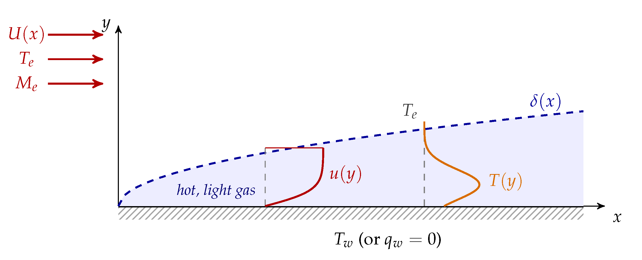
Figure 2.
Steady limit of the master system, Eqs. (38)–(), solved as a two-point boundary-value problem with , and an adiabatic wall. (a) With the momentum equation decouples from the energy equation and the velocity profiles for all collapse exactly onto the Blasius profile in the Dorodnitsyn plane, with independently of Mach number. (b) Temperature profiles; the wall value is the recovery temperature. (c) The same velocity profiles mapped back to the physical plane through : all of the compressible thickening resides in this mapping. (d) Effect of the pressure-gradient parameter at .
Figure 2.
Steady limit of the master system, Eqs. (38)–(), solved as a two-point boundary-value problem with , and an adiabatic wall. (a) With the momentum equation decouples from the energy equation and the velocity profiles for all collapse exactly onto the Blasius profile in the Dorodnitsyn plane, with independently of Mach number. (b) Temperature profiles; the wall value is the recovery temperature. (c) The same velocity profiles mapped back to the physical plane through : all of the compressible thickening resides in this mapping. (d) Effect of the pressure-gradient parameter at .
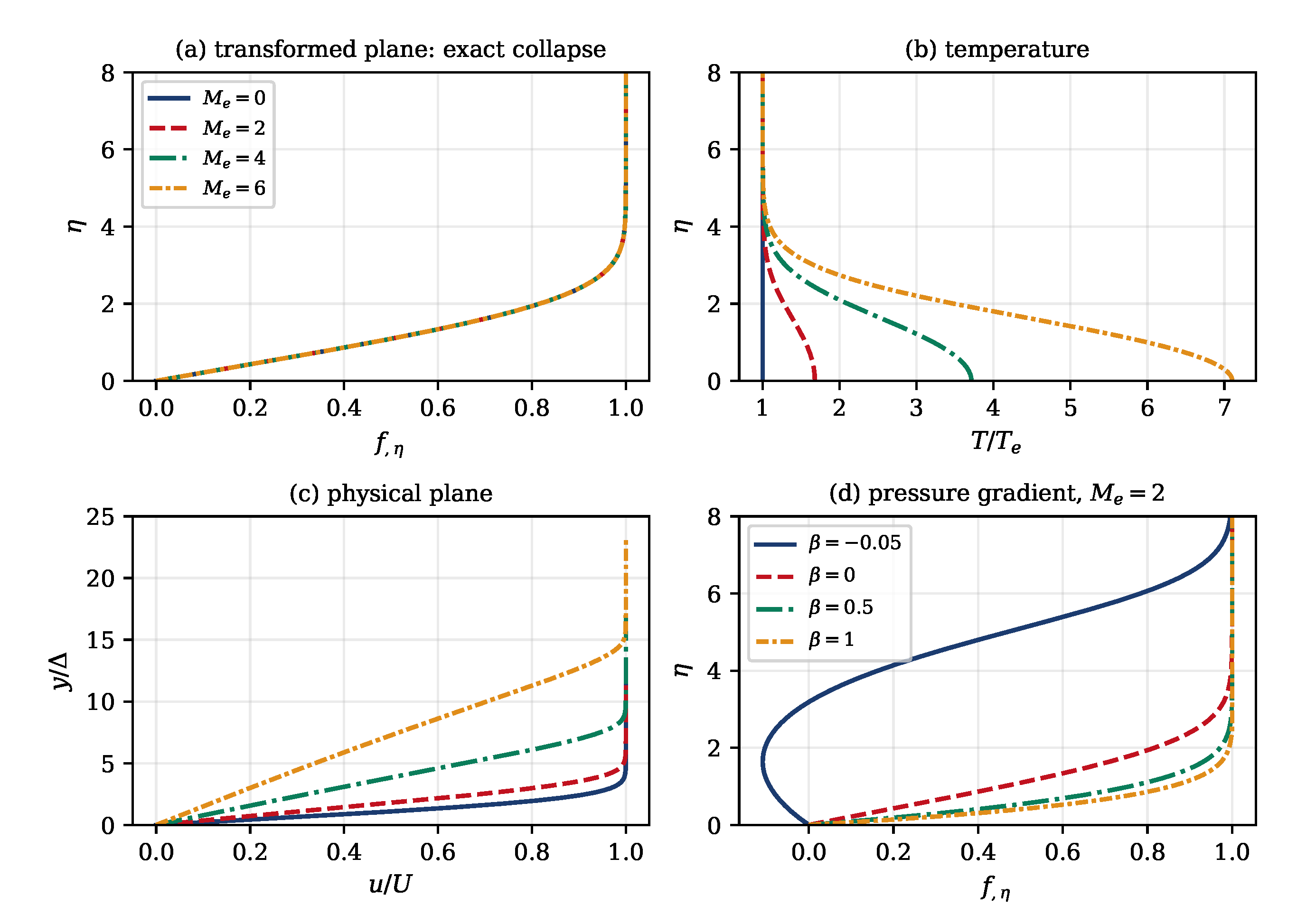
Figure 3.
Kummer branch of the compressible flat-plate problem. (a) The similarity function and its derivatives at . (b) Velocity profiles ; the plateau at large is the residual , which vanishes only as .
Figure 3.
Kummer branch of the compressible flat-plate problem. (a) The similarity function and its derivatives at . (b) Velocity profiles ; the plateau at large is the residual , which vanishes only as .
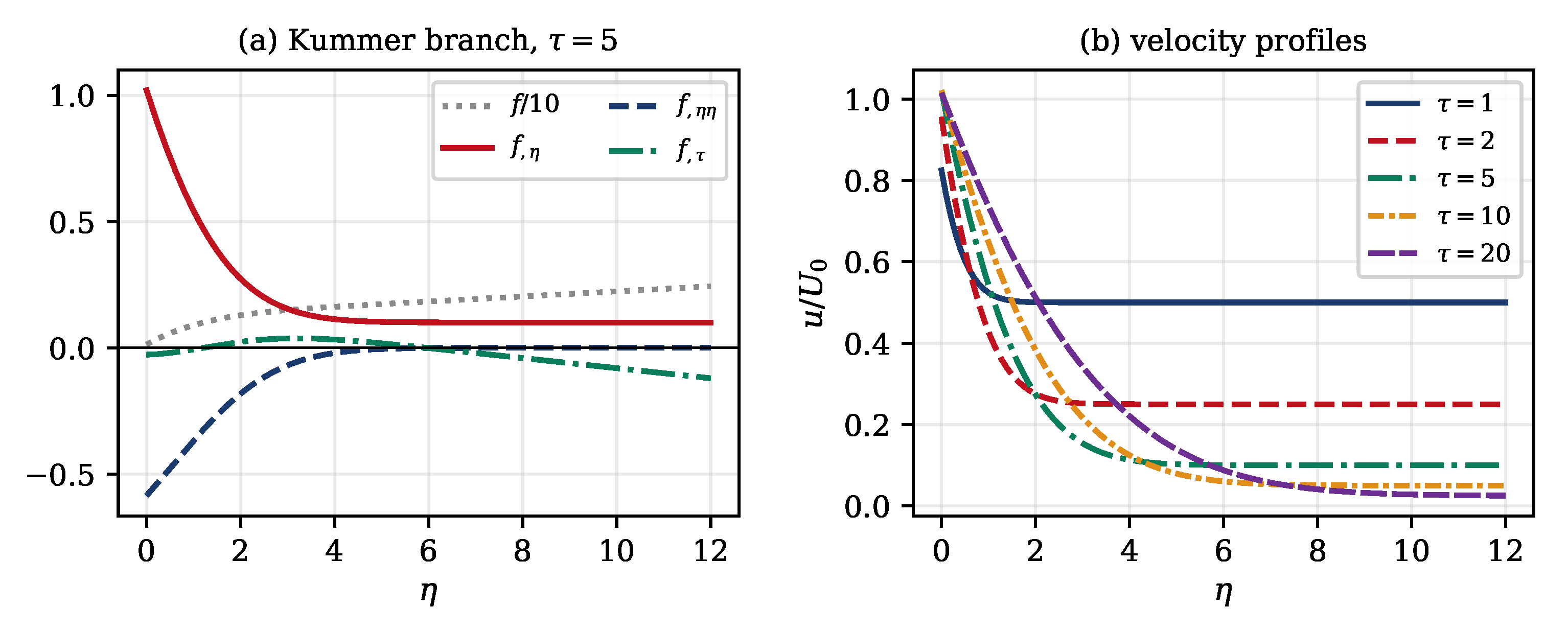
Figure 6.
Temperature field of the compressible impulsively started plate on the diffusive branch. (a) Adiabatic wall at , Eq. (56), for several wall Mach numbers. (b) Cooled, isothermal and heated walls at , Eq. (57). (c) Effect of Prandtl number on the adiabatic profile at , from the quadrature (60); the wall value is the recovery temperature (61).
Figure 6.
Temperature field of the compressible impulsively started plate on the diffusive branch. (a) Adiabatic wall at , Eq. (56), for several wall Mach numbers. (b) Cooled, isothermal and heated walls at , Eq. (57). (c) Effect of Prandtl number on the adiabatic profile at , from the quadrature (60); the wall value is the recovery temperature (61).
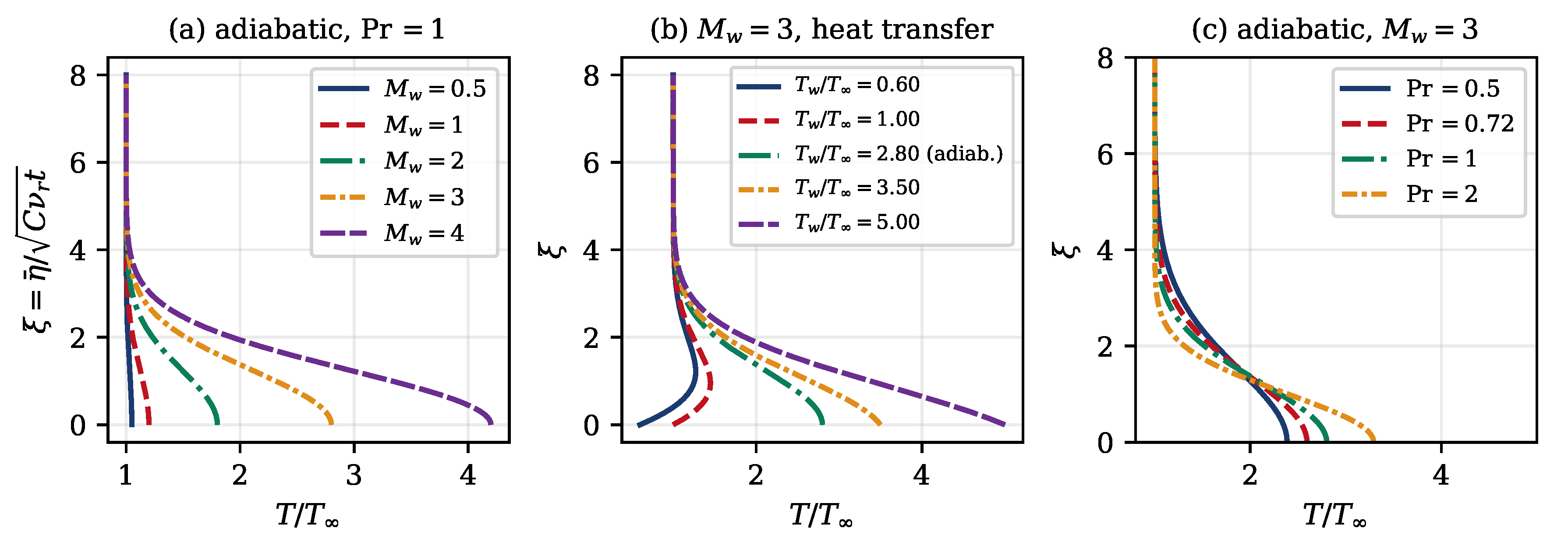
Figure 7.
(a) Adiabatic recovery factor. Solid line: closed form (61) for the unsteady Rayleigh layer; circles: numerical quadrature of (59); dashed line: ; squares: numerical solution of the steady system (38)–(). The two families cross at , where both equal unity. (b) Adiabatic wall temperature versus Mach number.
Figure 7.
(a) Adiabatic recovery factor. Solid line: closed form (61) for the unsteady Rayleigh layer; circles: numerical quadrature of (59); dashed line: ; squares: numerical solution of the steady system (38)–(). The two families cross at , where both equal unity. (b) Adiabatic wall temperature versus Mach number.
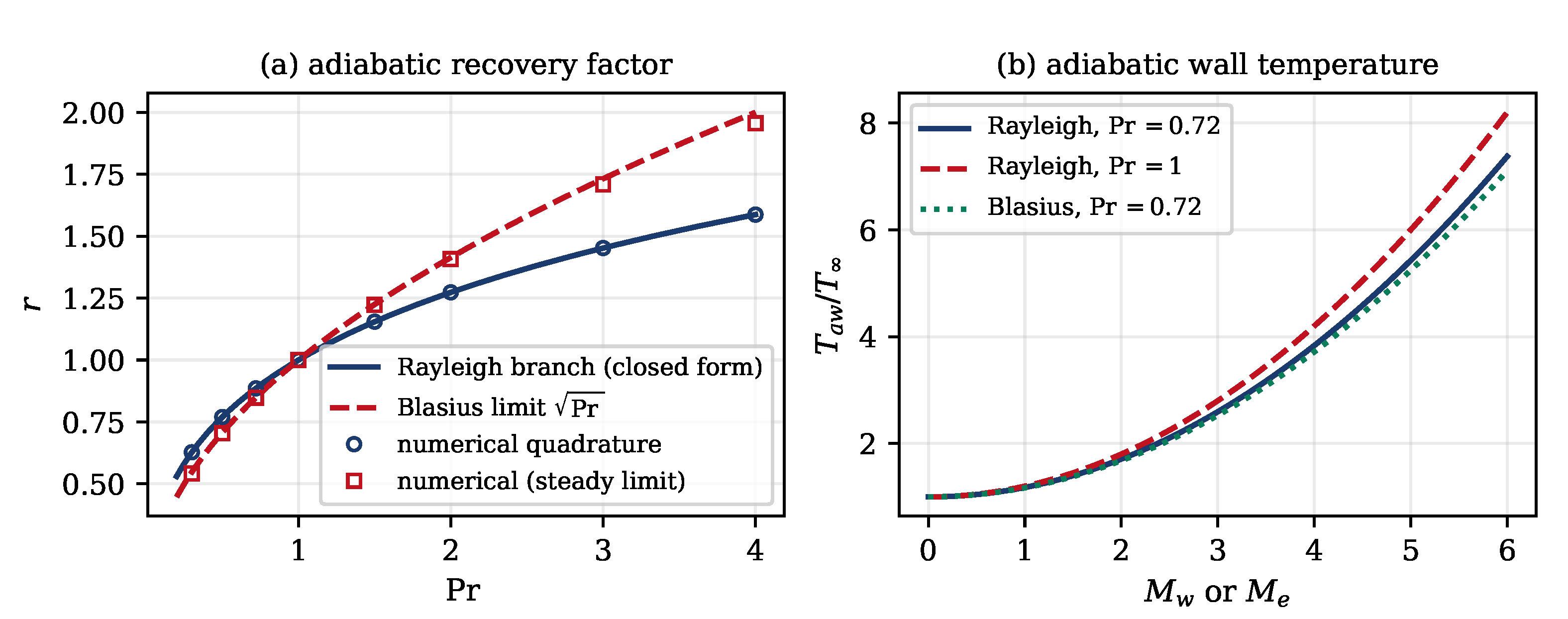
Figure 8.
The compressible impulsively started plate mapped back to physical coordinates by (82), adiabatic wall, . (a) Velocity; (b) density. In the Dorodnitsyn plane all curves would collapse onto the single profile ; the spreading seen here is entirely a consequence of the density defect produced by dissipative heating.
Figure 8.
The compressible impulsively started plate mapped back to physical coordinates by (82), adiabatic wall, . (a) Velocity; (b) density. In the Dorodnitsyn plane all curves would collapse onto the single profile ; the spreading seen here is entirely a consequence of the density defect produced by dissipative heating.
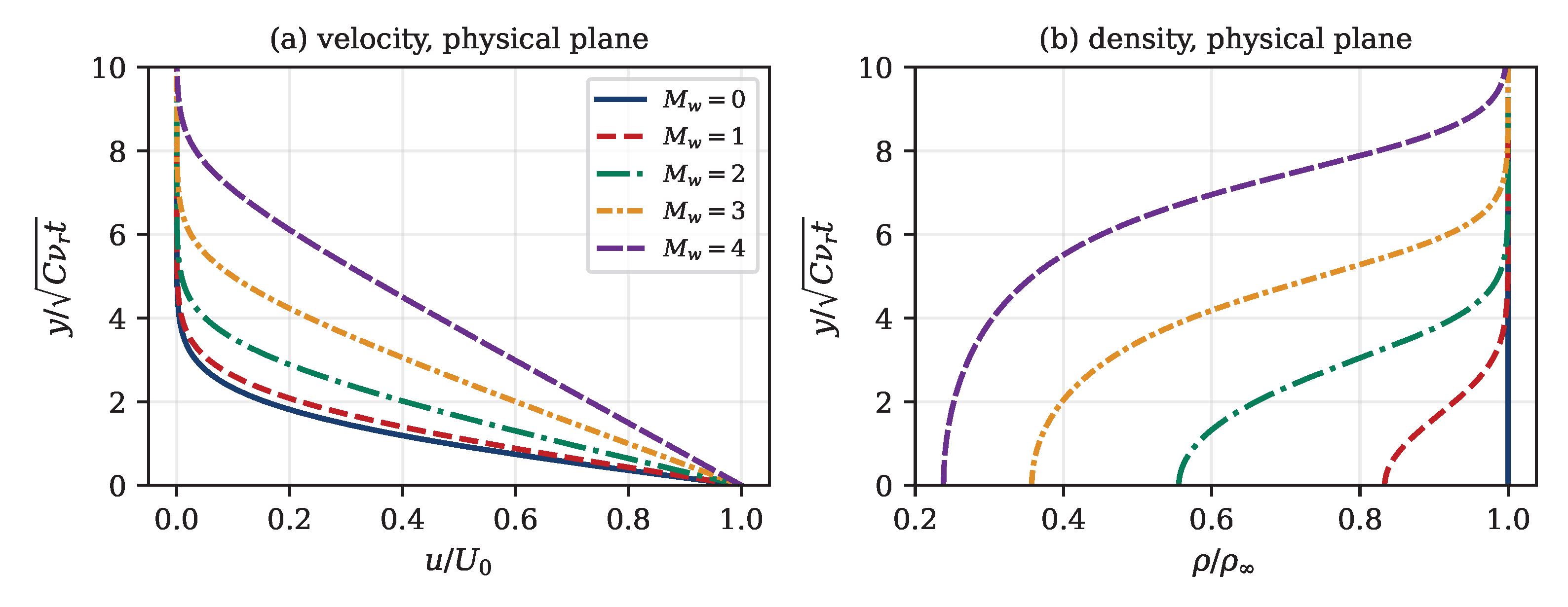
Figure 9.
Global solution of (85)–(), , adiabatic wall. (a) Velocity profiles from the Rayleigh start to the steady state. (b) Transformed wall shear: for it falls slightly below the Rayleigh value, for it rises steeply. (c) The coupling: at the curves for , 2, 4 collapse exactly (faint lines), whereas at they separate strongly. (d) The recovery factor migrates from the unsteady closed form (61) at to at when , and overshoots below it when .
Figure 9.
Global solution of (85)–(), , adiabatic wall. (a) Velocity profiles from the Rayleigh start to the steady state. (b) Transformed wall shear: for it falls slightly below the Rayleigh value, for it rises steeply. (c) The coupling: at the curves for , 2, 4 collapse exactly (faint lines), whereas at they separate strongly. (d) The recovery factor migrates from the unsteady closed form (61) at to at when , and overshoots below it when .
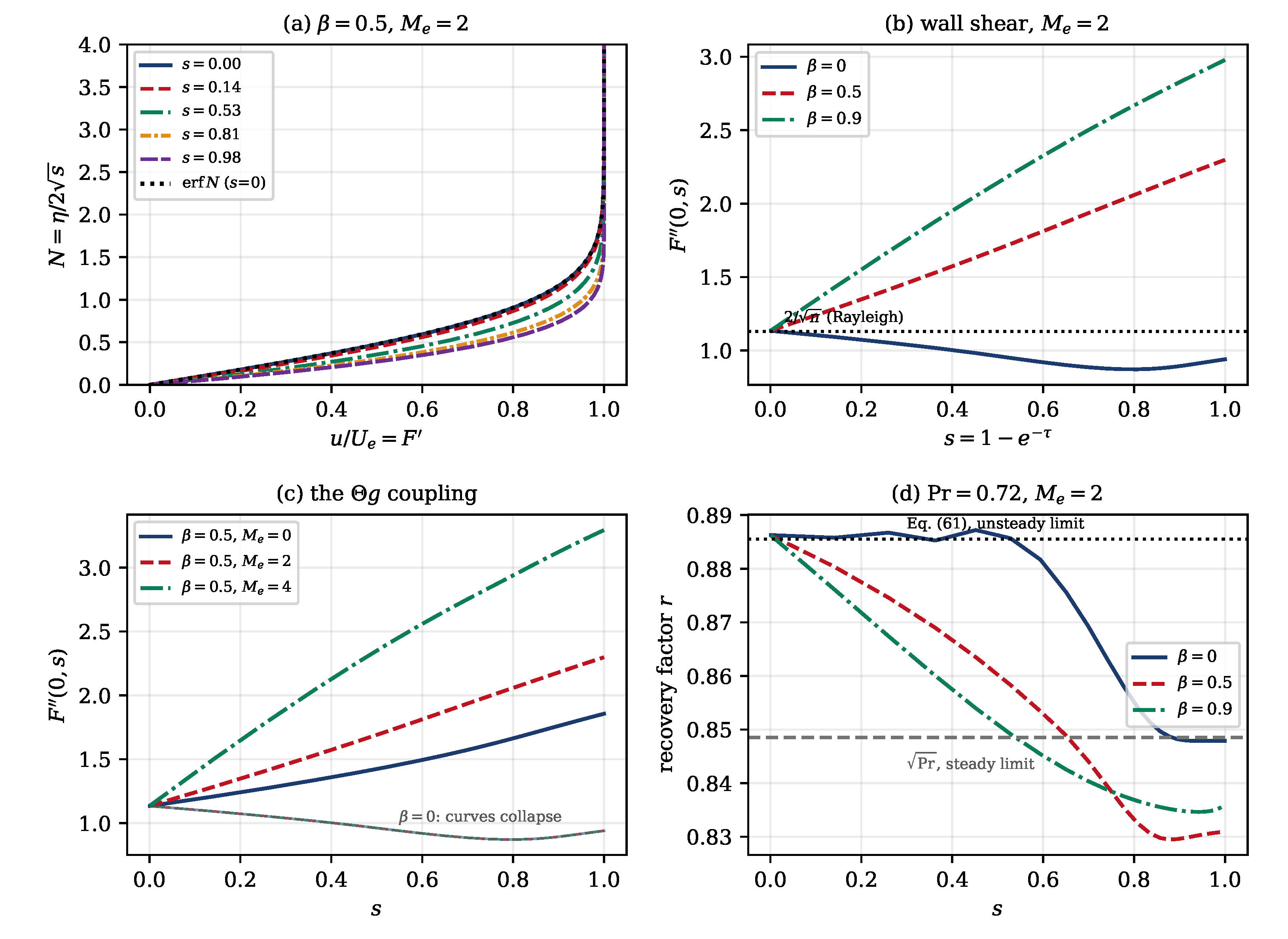

Table 1.
Parameters entering the two-dimensional unsteady compressible boundary layer in the Dorodnitsyn plane, and their dimensions.
Table 1.
Parameters entering the two-dimensional unsteady compressible boundary layer in the Dorodnitsyn plane, and their dimensions.
| Parameter | Dimension |
|---|---|
| (Dorodnitsyn normal coordinate) | L |
| t (time) | T |
| (transformed layer thickness) | L |
| (effective kinematic viscosity) |
Table 2.
Similarity transformations for unsteady boundary layers. The last row is the present compressible transformation; it contains the incompressible transformation of Ref. [15] as the limit , , , .
Table 2.
Similarity transformations for unsteady boundary layers. The last row is the present compressible transformation; it contains the incompressible transformation of Ref. [15] as the limit , , , .
| Author / flow | Transformation | Reduced equation |
|---|---|---|
| Stewartson[8] Secs. 5–6, incompressible, const | , | |
| Stewartson[8] Section 7, compressible, const, , , adiabatic | , , | , plus the Crocco integral; solved for only |
| Dennis[12] (numerical), const | , | |
| Sun[15], incompressible, | , | |
| Present, compressible, | , , | |
| together with the enthalpy equation (32) |
Table 3.
Steady limit, , , adiabatic wall, . and are the physical-plane thickness and displacement thickness in units of .
Table 3.
Steady limit, , , adiabatic wall, . and are the physical-plane thickness and displacement thickness in units of .
| 0 | 1.00 | 1.00000 | 1.000 | 3.473 | 03.473 |
| 2 | 1.80 | 0.93232 | 1.678 | 3.473 | 04.714 |
| 4 | 4.20 | 0.88397 | 3.713 | 3.473 | 08.437 |
| 6 | 8.20 | 0.86628 | 7.104 | 3.473 | 14.641 |
Table 4.
Adiabatic recovery factor of the compressible impulsively started plate from the closed form (61), compared with numerical quadrature of (59) and with the steady (Blasius) value .
| r Eq. (61) | r numerical | ||
|---|---|---|---|
| 0.50 | 0.76980 | 0.76980 | 0.70711 |
| 0.72 | 0.88550 | 0.88550 | 0.84853 |
| 1.00 | 1.00000 | 1.00000 | 1.00000 |
| 1.50 | 1.15470 | 1.15470 | 1.22474 |
| 2.00 | 1.27324 | 1.27324 | 1.41421 |
| 5.00 | 1.69588 | 1.69588 | 2.23607 |
Table 5.
Adiabatic recovery factor on the two branches. Column 2: Eq. (74), group-invariant solution on the Kummer branch; column 3: Eq. (61), diffusive branch; column 4: steady Blasius value. At the Crocco integral (55) gives on both branches, which the Kummer entry does not reproduce; see the text.
Table 5.
Adiabatic recovery factor on the two branches. Column 2: Eq. (74), group-invariant solution on the Kummer branch; column 3: Eq. (61), diffusive branch; column 4: steady Blasius value. At the Crocco integral (55) gives on both branches, which the Kummer entry does not reproduce; see the text.
| Eq. (74) | r Eq. (61) | ||
|---|---|---|---|
| 0.50 | 0.98276 | 0.76980 | 0.70711 |
| 0.72 | 1.14008 | 0.88550 | 0.84853 |
| 1.00 | 1.29824 | 1.00000 | 1.00000 |
| 1.50 | 1.51584 | 1.15470 | 1.22474 |
| 2.00 | 1.68561 | 1.27324 | 1.41421 |
| 5.00 | 2.31191 | 1.69588 | 2.23607 |
Table 6.
Validation of the present formulation. “Present” values are computed from the equations of this paper; “established” values are the accepted results of the cited sources. The Falkner–Skan entries are converted from the normalisation used here to the conventional .
Table 6.
Validation of the present formulation. “Present” values are computed from the equations of this paper; “established” values are the accepted results of the cited sources. The Falkner–Skan entries are converted from the normalisation used here to the conventional .
| Test case | Quantity | Present | Established |
|---|---|---|---|
| Blasius, , | [2,32] | ||
| Stagnation point, | [3,33] | ||
| Falkner–Skan, | [34] | ||
| Flat plate, , adiabatic | exactly | (Crocco integral) [26,27] | |
| Flat plate, , any | Mach independent | Mach independent [23,24] | |
| Steady layer, | recovery factor r | [30] | |
| Rayleigh layer, | r | 1 exactly | 1 [35] |
| Rayleigh layer, wall shear | [35,36] | ||
| Compressible Rayleigh | outflow | identical, Eq. (7.25) of [8] |
Table 7.
Global unsteady solution, , , adiabatic wall, grid. The two limits are compared with the exact Rayleigh value and with the independent steady solution of Section 4 (quoted as , the conversion implied by , ).
Table 7.
Global unsteady solution, , , adiabatic wall, grid. The two limits are compared with the exact Rayleigh value and with the independent steady solution of Section 4 (quoted as , the conversion implied by , ).
| steady | ||||
|---|---|---|---|---|
| 1.13093 | 0.30502 | 0.30399 | 0.86380 | |
| 1.13120 | 0.93948 | 0.93920 | 0.84779 | |
| 1.13188 | 1.74740 | 1.74603 | 0.83054 | |
| 1.13254 | 2.29486 | 2.29054 | 0.82403 | |
| 1.13321 | 2.73689 | 2.72805 | 0.82214 | |
| 1.13360 | 2.97146 | 2.95920 | 0.82234 |
Disclaimer/Publisher’s Note: The statements, opinions and data contained in all publications are solely those of the individual author(s) and contributor(s) and not of MDPI and/or the editor(s). MDPI and/or the editor(s) disclaim responsibility for any injury to people or property resulting from any ideas, methods, instructions or products referred to in the content. |
© 2026 by the authors. Licensee MDPI, Basel, Switzerland. This article is an open access article distributed under the terms and conditions of the Creative Commons Attribution (CC BY) license (http://creativecommons.org/licenses/by/4.0/).
Copyright: This open access article is published under a Creative Commons CC BY 4.0 license, which permit the free download, distribution, and reuse, provided that the author and preprint are cited in any reuse.