

Submitted:
20 August 2026
Posted:
21 August 2026
You are already at the latest version
Abstract
We present a self-contained formulation of finite-deformation Kirchhoff–Love shell theory built directly on the differential-geometric objects that the problem itself supplies: the shell body is a fibre bundle π : S → M over the mid-surface, kinematics are expressed through pull-backs of the ambient metric, stresses are bundle-valued differential forms, and dimensional reduction is fibre integration. Working in an orthonormal moving coframe and using Cartan’s structure equations [14,24], all metric information is carried by the connection 1-forms, so that the Gauss and Codazzi–Mainardi conditions appear as the vanishing of a curvature 2-form rather than as separately imposed cons traints. The resulting membrane and bending strain measures are Green–Lagrange tensors, hence exactly invariant under the full Euclidean group; no small-rotation, moderate-rotation or shallowness hypothesis is used anywhere. Relative to the usual presentation of this material we (i) give the exact through-thickness expansion of the pulled-back metric, including the O(z2) remainder that is normally discarded silently, and the exact shifter determinant μ0(z) = 1 + 2Hz + Kz2; (ii) derive the constitutive resultants by honest fibre integration, which produces curvature-induced membrane–bending coupling of relative size O(h2K) absent from the classical uncoupled form; (iii) derive the strong form of the balance laws from the variational statement and exhibit the shear–curvature coupling and the effective membrane resultant \(\hat N^{ab}=N^{ab}+M^{ac}\tilde b_{c}{}^{b}\) that are frequently omitted; (iv) supply the Kirchhoff boundary conditions with corner forces, which are unavoidable for a C1 shell theory; and (v) show explicitly how Koiter’s linear theory, the von Kármán plate equations, the Föppl membrane and inextensional bending are recovered as limits. The theory is then exercised numerically. Finiterotation invariance of the strain measures is confirmed to machine precision (∼ 10−17) on a generic doubly curved patch, against which the corresponding linearised measures accumulate spurious strain growing like 1 − cos θ—already 0.3% at 5◦, equivalent to 207MPa of fictitious stress in aluminium. A C1 Hermite discretisation of the axisymmetric reduction reproduces the classical clamped-circular-plate solutions in both the linear and large-deflection regimes, converges at the expected rate, and traces thecomplete snap-through equilibrium paths of clamped spherical caps, including the vanishing of the fundamental vibration frequency exactly at the limit points.
Keywords:
Kirchhoff–Love shell theory
; finite-deformation
; differential-geometric formulation
; membrane-bending coupling
; snap-through equilibrium paths
1. Introduction
Shell theory occupies an awkward position between three-dimensional continuum mechanics and the geometry of surfaces. The classical engineering literature [16,30,34,52] reaches the field equations by a sequence of coordinate manipulations in which the geometric content—what is a tensor, what is a connection, what is merely a coordinate artefact—is progressively obscured. Two costs follow. First, the compatibility conditions of Gauss and Codazzi–Mainardi have to be imposed by hand as extra equations, when they are in fact identities. Second, and more seriously for computation, the strain measures produced by displacement-based derivations are frequently only approximately invariant under rigid rotation, so that a rotating but unstrained shell element registers a fictitious strain. In an explicit dynamic computation, or in a buckling analysis where the physical membrane strains are themselves of order , this is not a small matter: Section 10.1 shows the effect is measured in hundreds of megapascals.
Both costs disappear if one takes the geometry seriously from the start. The observation organising this paper is that a shell is a fibre bundle. The mid-surface is the base, the through-thickness coordinate parameterises the fibre , and the shell body is the total space. Everything then falls into place:
- Kinematics is the pull-back of the ambient Euclidean metric along the deformation. Because a pull-back of a metric is manifestly invariant under isometries of the target, objectivity is automatic rather than a property to be checked.
- Geometry of the reference state is encoded in an orthonormal moving coframe and its connection 1-forms . Cartan’s structure equations [14] then deliver the Gauss and Codazzi–Mainardi relations as the statement that a certain curvature 2-form vanishes, because the reference configuration is embedded in flat .
- Stress is a vector-bundle-valued 2-form, its exterior covariant derivative is the divergence, and Cauchy’s theorem is Stokes’ theorem.
- Dimensional reduction is integration over the fibre. The resultants and are the zeroth and first fibre moments, and no assumption beyond the Kirchhoff–Love constraint is required to obtain them.
- What is new here.
The bundle picture is not itself new. Intrinsic, coordinate-free formulations of shell theory go back to Koiter [25,26], Naghdi [34] and Sanders [39]; the geometrically exact stress-resultant models of Simo, Fox and Rifai placed the theory squarely in the language of configuration manifolds, with the configuration space taken to be the manifold of maps into and the rotation of the director realised as motion on the unit sphere: Part I [41,48] formulates the model and its parametrisation—optimal in the precise sense that no smaller set of parameters describes the director field without introducing singularities ([41], §1.2(i))— ([42], Part II) develops the linear theory and the mixed interpolation, and Part III [43] carries both into the finite-deformation range; Libai and Simmonds [28] and Antman [2] give the definitive treatments of the nonlinear theory; and Ciarlet [9] and Marsden and Hughes [33] supply the differential-geometric apparatus. Rigorous justifications of two-dimensional models as limits of three-dimensional elasticity are given by Fox, Raoult and Simo [15] and Steigmann [47].
The contribution of this paper is to carry it through in complete detail, to correct a family of errors that recur in presentations of this kind, and to close the loop with a verified computation. Specifically, we draw attention to the following points, each of which is a place where published derivations are commonly wrong or incomplete.
- (i)
- The variation of the bending strain is not with free; under the Kirchhoff–Love constraint is a function of , and the correct result (Proposition 4) is with the current-surface connection.
- (ii)
- The linear-momentum balance is not . The correct tangential equation carries a shear–curvature coupling term and the effective resultant (Section 5.4). The necessity of an effective resultant is classical. Simo and Fox ([41], §1.2(viii), Eqs. (4.24)–(4.27)) obtain the companion result for the one-director Cosserat surface: balance of angular momentum forces the combination to be symmetric while itself is not, and it is this effective resultant, not , that is conjugate to the membrane strain rate in the reduced stress power ([41], Cor. 5.2). Part II states the same conclusion in the form used below: the constitutive restriction imposed by angular-momentum balance ([42], Equation (2.4)) defines the effective resultants ([42], Equation (2.5)), and only the symmetric effective membrane resultant survives in the weak form ([42], Equation (2.12)). The resultants themselves cannot be symmetric in the presence of initial curvature [34,35], ([42], §1(i)). The term is nevertheless routinely dropped in derivations that proceed by analogy with plate theory.
- (iii)
- Because the shell theory is of second differential order in , the boundary term does not separate into independent shear and twist; it must be integrated by parts along , producing the Kirchhoff effective shear and concentrated corner forces (Section 6).
- (iv)
- Fibre integration of the exact volume form with produces a membrane–bending coupling stiffness and corrections to the extensional and flexural stiffnesses, which vanish only in the limit (Section 5). Such curvature-induced terms are not new—they are given by Simo, Fox and Rifai ([42], Table 2) as a “higher-order constitutive model” obtained by asymptotic expansion—but the route here is different, and comparing the two exposes a consistency requirement that is easy to miss (Section 7.2).
- (v)
- Elementary but consequential: the resultant constitutive law is , not with and already containing ; the latter double-counts the modulus.
- Relation to computational practice.
The regularity that the Kirchhoff–Love constraint demands (Remark 4) has driven much of the recent finite-element literature: subdivision-surface elements [10,11] and isogeometric analysis [19,23] both exist largely to supply it. The alternative is to give up altogether by carrying an independent director with its own rotational degrees of freedom—the route taken by the degenerated-solid elements descending from Ahmad, Irons and Zienkiewicz [1] and by the one-director Cosserat models of [41,42,43]. The price is a shear-flexible kinematics with five degrees of freedom per node and, with it, the problem of updating a rotation exactly. Part III [43] settles that problem in closed form: since the director is a point of , its update is the exponential map along a great circle, which is well conditioned for increments of arbitrary magnitude and needs none of the quaternion machinery required for rods [45]. The discrete version of that map is already in Part II, where the nodal director interpolation is built so that the interpolated director has unit length and the incremental rotation stays orthogonal to it throughout the element ([42], Props. 4.1–4.3); the alternative of interpolating a nodal rotation vector is rejected there precisely because extracting it requires careful use of quaternions to avoid singularities ([42], Rem. 4.4(2)).
It is worth being explicit that this is the opposite of the choice made here. Simo and Fox parametrise the weak form so that the Riemannian connection of the mid-surface never appears, on the grounds that Christoffel symbols and the second fundamental form are not readily available in a computational setting ([41], §1.2(vi)); Part II makes the point explicitly, noting that Christoffel symbols, the second fundamental form and covariant derivatives never appear in the field equations as they cast them ([42], §1(iii)). The present paper does the reverse, making the connection 1-forms the carriers of all metric information (Section 2). Neither choice is more correct; they optimise for different things—theirs for an element that can be coded without differential geometry, ours for a formulation in which compatibility is an identity rather than an imposed constraint. Section 10.10 compares the two where they overlap; the difference in kinematic hypothesis—shear-rigid here, shear-flexible there—is what fixes the sign of the residual discrepancy we find. Surveys of the competing discretisation strategies are given by Bischoff, Ramm and Irslinger [4] and Bathe [3]; standard benchmark problems for geometrically nonlinear shells are collected by Sze, Liu and Lo [49]. The present paper is not a finite-element paper, but Section 10 shows that the formulation discretises cleanly, that its theoretical guarantees survive discretisation, and that the consistent tangent it supplies delivers the asymptotically quadratic Newton convergence that such a tangent is supposed to deliver (Section 10.11).
- Outline.
Section 2 sets up the bundle, the moving frame and the structure equations. Section 3 develops the finite-deformation kinematics and the strain measures, with the objectivity proof and the exact truncation estimate. Section 4 introduces the bundle-valued stress forms and the three-dimensional virtual-work statement. Section 5 performs the fibre integration and derives the strong form; Section 6 the boundary conditions. Section 7 closes the system constitutively, Section 8 verifies that the classical theories are recovered as limits, and Section 9 gives the consistent tangent operator required for Newton solution. Section 10 is the numerical case study.
2. Geometric Foundations
2.1. The Shell as a Fibre Bundle
Definition 1
(Shell bundle). Let be a compact orientable 2-manifold with piecewise-smooth boundary, embedded in by with unit normal field . Let . The shell bundle is the trivial fibre bundle
(Figure 1) with reference embedding
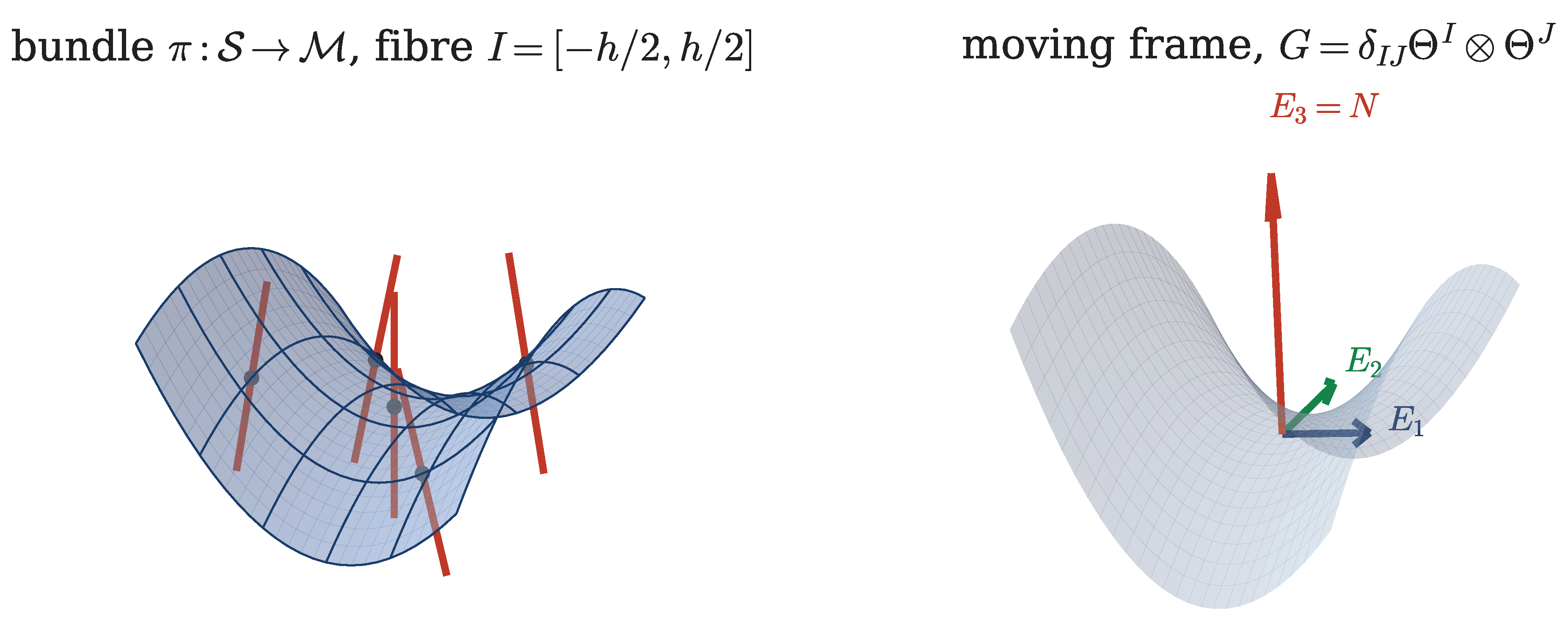
Figure 1.
The shell as a fibre bundle. Left: the mid-surface is the base, the fibres (red) are the through-thickness segments carried along the unit normal, and the total space is the shell body. Right: the orthonormal moving frame dual to the coframe (5), in which the pulled-back metric is and all geometric information is carried by the connection 1-forms .
Figure 1.
The shell as a fibre bundle. Left: the mid-surface is the base, the fibres (red) are the through-thickness segments carried along the unit normal, and the total space is the shell body. Right: the orthonormal moving frame dual to the coframe (5), in which the pulled-back metric is and all geometric information is carried by the connection 1-forms .
Remark 1.
is an embedding provided pointwise, i.e., : the thickness must not reach the focal surfaces. All statements below are made under this hypothesis, which is the precise form of the “thin shell” assumption at the level of geometry. It is weaker than the constitutive thinness assumption used later.
Triviality of the bundle is a convenience, not a restriction of substance: for a non-orientable mid-surface one works with the associated -bundle, and every formula below is local and therefore unaffected.
2.2. Moving Coframe and Connection Forms
Let be lines-of-curvature coordinates on with Lamé parameters and principal radii , so that the mid-surface first and second fundamental forms are
Remark 2
(Sign convention). We fix once and for all
so that with when the centre of curvature lies on the side. This is the convention forced on us by the metric expansion (18), and it is the opposite of the more common . Mixing the two is a frequent source of sign errors in the bending strain; we therefore never use the symbol b for a reference quantity, and write only where the outward-normal convention is genuinely wanted, namely in the normal equilibrium equation (40).
Define on the orthonormal coframe
so that the pull-back of the Euclidean metric along is
and the Riemannian volume form is
with the mean and the Gaussian curvature. The function is the determinant of the shifter that maps the mid-surface tangent plane onto the tangent plane of the parallel surface at height z; it is the exact Jacobian of the fibre coordinates and is retained throughout Section 5. Shifter tensors of this kind are standard in the shell literature [16,34] but are usually set to unity at the first opportunity.
Proposition 1
(Connection forms). The unique torsion-free metric connection 1-forms satisfying the first structure equation are
where and no summation is implied in .
Proof.
Antisymmetry is metric compatibility of (6). For : and , so the third structure equation holds identically. For ,
while , which cancels the second term exactly. The remaining requirement fixes the -component of as stated, and the companion equation for fixes the -component. Uniqueness is the fundamental lemma of Riemannian geometry. □
2.3. Curvature 2-Form; Gauss and Codazzi–Mainardi
Theorem 1
(Compatibility as flatness). Because and is flat, the curvature 2-form
vanishes identically. Its components are equivalent to the classical compatibility conditions of surface theory:
Equations (10)–(11) are the Codazzi–Mainardi equations and (12) is Gauss’ theorema egregium [13], .
Proof.
is an isometric embedding into flat space, so the induced Levi-Civita connection has vanishing curvature; (9) is the second Cartan structure equation. Substituting (8) and collecting the coefficients of and gives the stated component identities; note that the z-dependence cancels identically, which is precisely the statement that the parallel surfaces of a surface satisfying (10)–(12) again satisfy them. □
Remark 3.
This is the first concrete payoff of the formalism. In a coordinate treatment, (10)–(12) are three additional partial differential equations that must be appended to the field equations and then shown to be preserved. Here they are consequences of the ambient space being flat, and they are automatically satisfied by any configuration that is actually realised as a surface in —which is exactly the class of configurations a displacement-based formulation produces.
2.4. Exterior Covariant Derivative
For a -valued p-form on (components in the moving frame dual to ) the exterior covariant derivative is
Theorem 1 gives on , so the complex of bundle-valued forms is exact and Stokes’ theorem holds in the form
This identity is what replaces the divergence theorem in Section 4, and it is the reason no Christoffel symbols appear explicitly anywhere in the derivation of the balance laws.
3. Finite-Deformation Kinematics
3.1. Deformation and the Kirchhoff–Love Constraint
Let be the deformed mid-surface placement, assumed an immersion, and let
be the deformed unit normal. The shell deformation is
Remark 4
(On the status of ). It is common to see described as “an independent kinematic variable subject to the orthogonality constraint ”. These two statements are incompatible: once the constraint is imposed, is determined by through (15) and is not independent. Two consistent formulations exist [2,41]:
- (a)
- the constrained (Kirchhoff–Love) theory used here, with the single field and given by (15); or
- (b)
- a mixed theory with independent director and Lagrange multipliers enforcing , whose stationarity conditions recover (a) after elimination, and which relaxes to Reissner–Mindlin kinematics if the constraint is penalised [4]. The one-director Cosserat models of Simo, Fox and Rifai take the unconstrained limit of (b) as their starting point: the director is a free point of with two rotational degrees of freedom, so the kinematics is shear-flexible from the outset and no constraint is imposed ([42], §1(v)).
The distinction is not pedantic: it dictates the regularity required of the trial space ( versus ) and it changes the variation of the bending strain, Proposition 4.
3.2. Pull-Back Metric: Exact Expansion
Write for the deformed first fundamental form, , and, consistently with Remark 2,
Proposition 2
(Exact pull-back). With Φ as in (16),
and correspondingly with . The tensor is the third fundamental form and satisfies the Cayley–Hamilton identity .
Proof.
and . Taking inner products and using , , gives (18) with no remainder. The last identity is Cayley–Hamilton for the Weingarten map . □
Note that (18) is exact: no expansion has been performed. This matters for the error estimate below.
3.3. Strain Measures
Definition 2
(Membrane and bending strains).
These are the finite-strain counterparts of Koiter’s membrane and bending measures [25,39]; see also [36,40] for equivalent finite-rotation forms. Both are covariant 2-tensor fields on , i.e., sections of ; in particular they are ordinary tensors, not “pseudo-strains”, and they may be pushed forward, pulled back and differentiated covariantly without qualification.
Proposition 3
(Green–Lagrange strain of the shell body). The three-dimensional Green–Lagrange strain has components
The vanishing of the transverse strains is the Kirchhoff–Love hypothesis; it is a consequence of (16), not a separate assumption.
Corollary 1
(Truncation error). The thin-shell strain field used in Section 5 is , with pointwise error
uniformly on . Retaining is therefore consistent only if one also retains constitutive terms; we do so in Section 5 through but discard the strain remainder, which is the standard—and here explicitly quantified—Kirchhoff–Love truncation [26,47]. Section 10.2 confirms the quadratic rate numerically.
3.4. Exact Objectivity
Theorem 2
(Invariance under the Euclidean group). Let and be constants and let . Then
identically—not to any order in a rotation parameter.
Proof.
, hence because . Since , (15) gives , whence . Both reference quantities are untouched. □
Remark 5
(Why this is not automatic). Linear and moderate-rotation shell theories [26,52] replace by its first variation at the reference configuration, . For a rigid rotation this gives
where θ is the rotation angle and the projector orthogonal to the rotation axis. The spurious strain therefore grows like : at , at , at . Section 10.1 confirms (23) numerically and converts it into fictitious stress.
3.5. Admissible Variations
Let be a variation. Because is slaved to , its variation is determined.
Lemma 1
(Variation of the normal).
Proof.
gives , so is tangential, . Varying gives , i.e., . Invert. □
Proposition 4
(Strain variations). With the Levi-Civita connection of the deformed metric (Christoffel symbols ),
Remark 6
(A common error). It is sometimes written that . The right-hand side is identically zero, since the third term is by the product rule the sum of the first two. The correct statement is (26). The presence of —the deformed, not reference, Christoffel symbol—is what makes a tensor, and it is exactly the term that a naive derivation loses.
4. Stress as a Bundle-Valued Form; Virtual Work
4.1. The Piola Stress 2-Form
Let be the first Piola–Kirchhoff stress of the three-dimensional body, a two-point tensor. Its natural differential-geometric avatar is the -valued 2-form
so that for any surface with unit normal the traction resultant is . Equivalently , the Hodge dual taken in the reference metric (6).
Proposition 5
This is the shell-theoretic instance of the general geometric formulation of continuum mechanics in [33]. Balance of angular momentum is, in this language, the statement that the -valued 3-form has vanishing skew part, which is equivalent to symmetry of the second Piola–Kirchhoff stress .
4.2. Three-dimensional virtual work
Everything that follows is obtained from (30) by fibre integration; no further mechanical assumption is introduced.
5. Dimensional Reduction by Fibre Integration
5.1. Resultants
Using Proposition 3 with the truncation of Corollary 1, , and the exact volume form (7),
which defines the resultants as the weighted fibre moments
The weight is the exact shifter determinant; setting is an additional approximation of relative order which we do not make.
5.2. Exact Through-Thickness Stiffness
With the linear-elastic law of Section 7 and , the elementary integrals
give the exact resultant constitutive law
Remark 7
(Curvature-induced coupling). Even for a homogeneous isotropic shell, initial curvature produces a membrane–bending coupling , of relative size compared with . This is a purely geometric effect—the outer fibres of a curved shell are longer than the inner ones—and it is invisible in formulations that set . For the caps of Section 10, and the effect is negligible, as it should be; for thick pressure-vessel heads or laminated tubes with it is not.
5.3. Inertia
Fibre integration of the inertial term in (30), using , gives
The last term is the rotary inertia, of relative size where L is the shortest deformation wavelength; it is retained here for completeness and neglected in Section 10, where .
5.4. Strong Form
Theorem 3
(Local balance laws). Define the difference tensor between the deformed and reference Christoffel symbols (a genuine -tensor), the effective membrane resultant and the effective shear
indices on being raised with , and the stress vector
Then (30) is equivalent to the vector balance law
on , whose tangential and normal projections read
Proof.
Insert (25)–(26) into (31). Since is compatible with but is not, write , so that
Integrating the second term by parts once and using the Weingarten relation collects the tangential parts into and the normal parts into , yielding . A second integration by parts and the fundamental lemma give (38). Projecting on and , and using , gives (39)–(40). The omitted terms “…” are the - and -weighted director inertias of (35). □
Remark 8
(What is usually missing). Three features of Theorem 3 are commonly absent from presentations of Kirchhoff–Love shell theory, though all three are present in the careful treatments [28,34,41]:
- (a)
- the replacement of by , which is what makes the true traction vector;
- (b)
- the shear–curvature coupling in the tangential equation (39). Writing simply is correct only for a flat plate;
- (c)
- the term in , which is and hence negligible in small-strain/large-rotation regimes but must be present for the formulation to be exactly variationally consistent (and therefore for Newton’s method to converge quadratically).
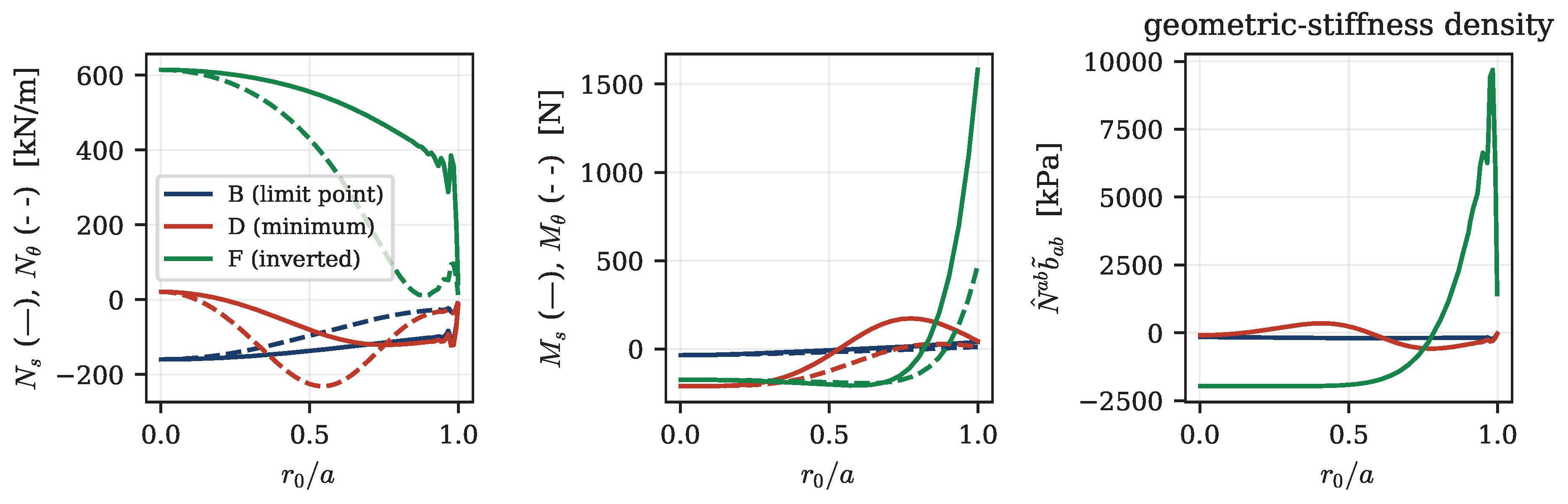
The term in (40) is the geometric-stiffness density: it is the mechanism by which membrane compression destabilises a curved shell, and it is what produces the limit points computed in Section 10.8.
6. Boundary Conditions and Corner Forces
The boundary term generated in the proof of Theorem 3 is
with the outward unit conormal and the unit tangent of . Because and its tangential derivative along are not independent, (41) must be reduced further. Decomposing and writing , , integration by parts along gives
Proposition 6
(Kirchhoff boundary conditions).
so that the natural (traction) boundary conditions are
and the essential conditions are prescription of and of the normal slope .
Remark 9.
The corner forces are not an artefact. A Kirchhoff–Love shell has three boundary conditions per edge, not four, and the twisting moment cannot be prescribed independently of the shear; the concentrated corner reactions are what restores consistency. Any formulation that lists four independent edge conditions is over-determined. The work-conjugate structure of shell boundary conditions at finite rotation is analysed in detail by Makowski and Pietraszkiewicz [31]. The clamped conditions used in Section 10 ( and prescribed) are essential throughout, so no corner forces arise there; they would for a simply-supported polygonal panel.
7. Constitutive Closure
7.1. Plane-Stress Condensation
Take a Saint-Venant–Kirchhoff material with strain energy per unit reference volume , the Lamé parameters. The Kirchhoff–Love kinematics forces but leaves undetermined; it is fixed by the plane-stress condition , which gives
and substituting back replaces by the reduced modulus .
Proposition 7
(Reduced elasticity tensor).
components referred to the orthonormal coframe .
Remark 10
(Dimensional consistency). already carries the modulus and has units of stress. The resultant law is therefore
with from (34). Writing instead with —as is occasionally seen—multiplies the modulus in twice and produces membrane stiffnesses too large by the factor .
In the thin-shell limit , , , , and (46) collapses to the familiar uncoupled form with extensional and flexural rigidities
7.2. Comparison with the Higher-Order Model of Simo, Fox and Rifai
Simo, Fox and Rifai ([42], Table 2) give a higher-order resultant constitutive model obtained by asymptotic expansion of the three-dimensional stored energy, in which the membrane and bending resultants read
with linear in the second fundamental form , quadratic in , and linear in the third fundamental form —which is exactly the tensor of Proposition 2. Three features of (48) should be recorded before any comparison is attempted.
- (i)
- The conventions coincide. Their second fundamental form is our of (4), and their bending measure ([42], Equation (2.11c)) is our (Definition 2) verbatim, the director replacing the normal . No sign reconciliation is needed, and the discrepancies found below are therefore real and not artefacts of Remark 2.
- (ii)
- (iii)
- The resultants are the effective ones. The quantities , , of Table 2 are the effective resultants defined by , ([42], Equation (2.5)), not the bare resultants of (34). Comparing the two requires converting one to the other, and at order the conversion is not negligible.
Specialising both models to a sphere of radius R, where , , , one finds , , , and , so that the coefficient of multiplying and in the membrane resultant is
The third row is and of (34) with , . All entries, together with the three tensor identities above, are verified symbolically in code/verify_table2.py.
Remark 11
(An inconsistent truncation, and its repair). Even between the two directly comparable rows of (49) the coupling coefficients differ by a factor of and the membrane correction by a factor of 6; against the effective resultant as tabulated the factors are and 10. Converting between effective and bare resultants therefore narrows the gap but does not close it, and by item (i) above the sign reversal cannot be attributed to conventions. The discrepancy is nevertheless not an error in either derivation; it is the truncation warned about in Corollary 1. Equation (34) retains the shifter exactly but discards the strain remainder , and both are of order . Retaining one without the other is inconsistent. Carrying both through the fibre integral gives, in place of (34),
with , and the -type term of (48) is recovered. That the two models should differ at this order is not a surprise on their side either: Simo and Fox derive the lowest-order relations by asymptotic expansion of the three-dimensional Saint-Venant–Kirchhoff model retaining terms through , and note explicitly that products of with the curvature parameters are of higher order and are conventionally discarded, so that the resultant law is left depending on the reference surface through its first fundamental form alone ([41], Rem. 5.5(2)); the general dependence of resultant constitutive laws on reference geometry is the subject of Carroll and Naghdi [8]. Equations (48) and (34) are two different partial retentions of the terms that expansion discards, which is why they disagree. The practical consequence is small: ([42], Remarks 2.2) report that the lowest-order and higher-order models give numerically indistinguishable results, and that through-thickness integration of three-dimensional laws “leads to no improved accuracy for most thin, or moderately thick, shell problems”. For the shells of Section 10, and every term in (49) beyond the leading h is below relative, so the factors of and 6 are without practical consequence here. The point is one of principle: (34) should be read as the -exact model, not as a consistent theory, and (50) is the consistent one.
Remark 12
(The third fundamental form as the carrier of the corrections). The same tensor appears in the third of the Table 2 relations, the transverse shear law ([42], Table 2). That the leading curvature correction to every resultant stiffness—membrane, coupling and shear—is carried by and by the shifter built from it is not a coincidence: by Proposition 2 the pull-back metric is exactly , so is the only new tensor that accuracy can produce. The present theory is shear-rigid and has no counterpart of , but the structural agreement is a useful check on (50).
7.3. Stored Energy and Hyperelasticity
The reduced two-dimensional stored-energy function is
with , . Because and are exactly objective (Theorem 2), is frame-indifferent by construction, and the resulting boundary-value problem is variational: for conservative loading, equilibria are the critical points of
This is what licenses the energy-based numerical treatment of Section 10, including the use of the second variation as a stability criterion.
8. Reduction to Classical Theories
A formulation of this generality is only trustworthy if the standard theories drop out of it. We record the four relevant limits; each is a statement about which terms are retained in , and Theorem 3.
- (i)
- Koiter’s linear shell theory.
Write and linearise (19) at :
With this is exactly Koiter’s energy [9,26]. The price is (23): the theory is no longer rotation-invariant.
- (ii)
- von Kármán plate.
Take flat, , retain quadratic terms only in w:
and (40) becomes , the von Kármán equation [52], with because is already second order.
- (iii)
- Föppl membrane.
Set . Then , (40) reduces to — the Young–Laplace law—and (39) to .
- (iv)
- Inextensional bending.
Impose . By Gauss’ theorema egregium (Theorem 1) [13] the deformation preserves K, so the admissible motions are the isometries of ; the energy reduces to . This limit is the correct description whenever and it is the reason that developable shells roll up at essentially zero membrane stress — behaviour that a formulation with spurious rotational strain cannot reproduce.
9. Linearisation and the Consistent Tangent
Newton solution of (52) requires the second variation. Writing , the tangent operator splits in the usual way into material and geometric parts:
with , , and
The geometric term is what carries the destabilising effect of membrane compression; dropping it (as in a “modified Newton” scheme) does not change the equilibrium path but destroys quadratic convergence and invalidates eigenvalue-based stability assessment. Both terms in (55) are symmetric, here because the loading is dead and the material hyperelastic, so that (55) is a second variation of . It is worth recording that symmetry survives in settings where that argument is unavailable: in the one-director Cosserat model the restriction that balance of angular momentum places on the admissible constitutive equations is by itself enough to make the consistent tangent symmetric even away from equilibrium ([41], §1.2(vii), Equation (6.34)). In Section 10 we obtain (55) to machine accuracy by complex-step differentiation of the discrete energy, which sidesteps the algebra entirely while remaining exact.
Remark 13
(Continuum versus discrete linearisation). Equation (55) is the linearisation of the continuum weak form, and it is not in general the tangent of the discrete problem. If the unknowns are interpolated nonlinearly—as they unavoidably are whenever a director or a rotation is interpolated on a manifold — linearisation and interpolation do not commute, so substituting the interpolation into (55) yields an operator that is only consistent to leading order ([43], Rem. 4.4); the correct object is the derivative of the discrete residual [44]. For the present discretisation the distinction is vacuous, since the unknown is itself and enters its nodal parameters linearly, so the two operations commute. It is nevertheless the reason the results below are obtained by differentiating the discrete energy rather than by discretising (55). Nor is the point cosmetic: an inexact tangent destroys the asymptotic quadratic rate (Section 10.11) and, more seriously, corrupts the detection of limit and bifurcation points, which are defined by singularity of the tangent itself ([43], Rem. 5.2).
A related trap is worth naming, because it has the same source. In the second variation it matters which object is held fixed. Here is not independent—it is determined by through the Kirchhoff–Love constraint (Proposition 4)—so acquires the second term in (55). The Cosserat counterpart is that the primitive variation is the rotation and not the director increment , so that while ([41], Rem. 6.3, [43], §2.2.1). In both cases treating the dependent quantity as free loses a term of the geometric tangent and with it the quadratic rate.
10. Numerical Case Study
This section does three things: it verifies the claims of Section 3 directly, it verifies a discretisation of the theory against classical closed-form results, and it applies the whole apparatus to a genuinely nonlinear problem—the snap-through of clamped spherical caps—including the dynamic signature of the instability.
Throughout, the material is aluminium: GPa, , kg m−3.
10.1. Verification of Exact Objectivity
Theorem 2 is tested on a generic doubly curved Monge patch
which has both elliptic and hyperbolic regions, non-orthogonal coordinate lines and non-constant curvature. All surface derivatives are computed analytically, so the only error present is floating-point round-off. The patch is subjected to with a generic axis and translation , and , are evaluated at .
Figure 2 shows the outcome. The exact measures sit at – relative, i.e., at the round-off floor, uniformly in —including at and , where no expansion-based theory retains any accuracy. The linearised measures reproduce (23) to graphical precision. Selected values are given in Table 1.
Figure 2.
Spurious strain generated by a pure rigid rotation of the doubly curved patch (57). (a) The Green–Lagrange measures of Definition 2 remain at round-off () over the full range –, while the corresponding linearised measures follow exactly, as predicted by (23). (b) The same data expressed as fictitious stress ; the yield stress of Al 7075-T6 is exceeded by the numerical artefact alone at about of rigid rotation.
Figure 2.
Spurious strain generated by a pure rigid rotation of the doubly curved patch (57). (a) The Green–Lagrange measures of Definition 2 remain at round-off () over the full range –, while the corresponding linearised measures follow exactly, as predicted by (23). (b) The same data expressed as fictitious stress ; the yield stress of Al 7075-T6 is exceeded by the numerical artefact alone at about of rigid rotation.
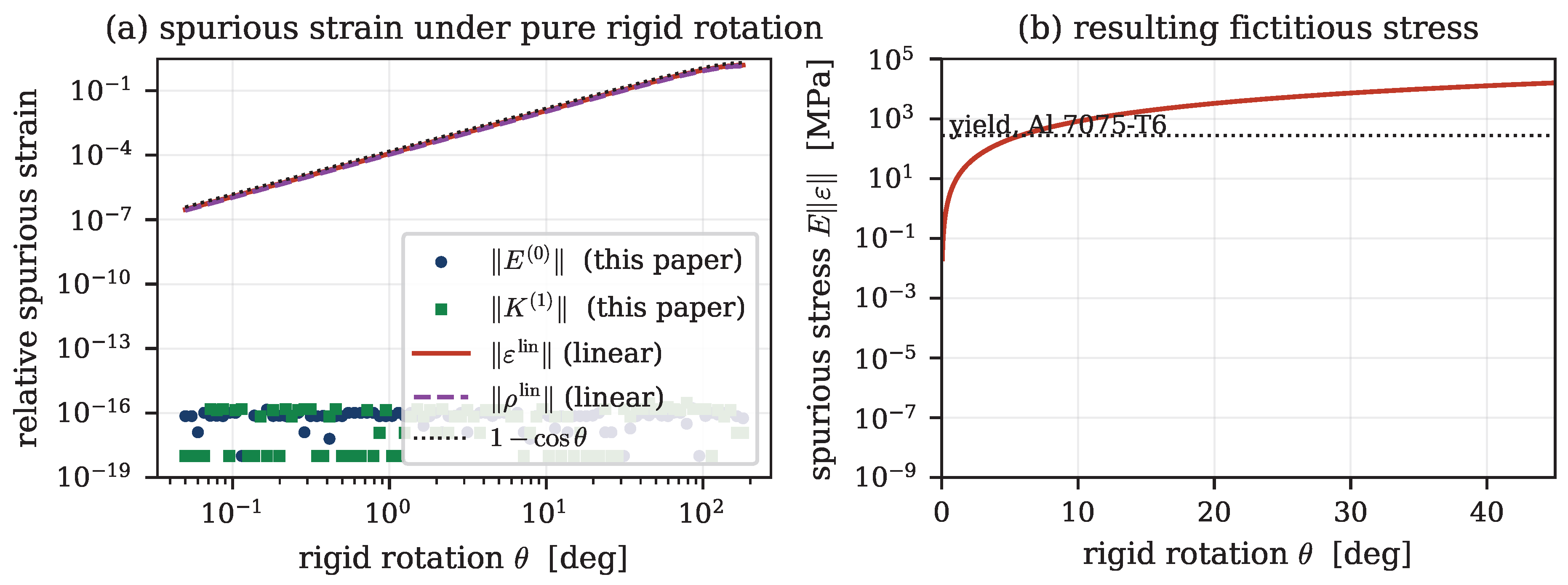

Table 1.
Relative spurious strain under rigid rotation of the patch (57). “Present” refers to of Definition 2; “linear” to of Remark 5. The last column is the equivalent fictitious stress .
Table 1.
Relative spurious strain under rigid rotation of the patch (57). “Present” refers to of Definition 2; “linear” to of Remark 5. The last column is the equivalent fictitious stress .
| [deg] | present | present | linear | fictitious stress [MPa] |
|---|---|---|---|---|
| 0.5 | 2.1 | |||
| 1.0 | 8.3 | |||
| 2.0 | 33 | |||
| 5.0 | 207 | |||
| 10.0 | 825 | |||
| 20.0 | 3277 | |||
| 45.0 | 15918 | |||
| 90.0 | 54341 |
The practical reading of Table 1 is the fourth row. A shell element rotating rigidly through —a routine occurrence in a buckling or crash calculation—acquires, in a linearised formulation, a spurious strain of . Physical membrane strains in a buckling shell are of exactly this order. The artefact is therefore not a small correction to the answer; it is the same size as the answer.
10.2. Verification of the Truncation Estimate
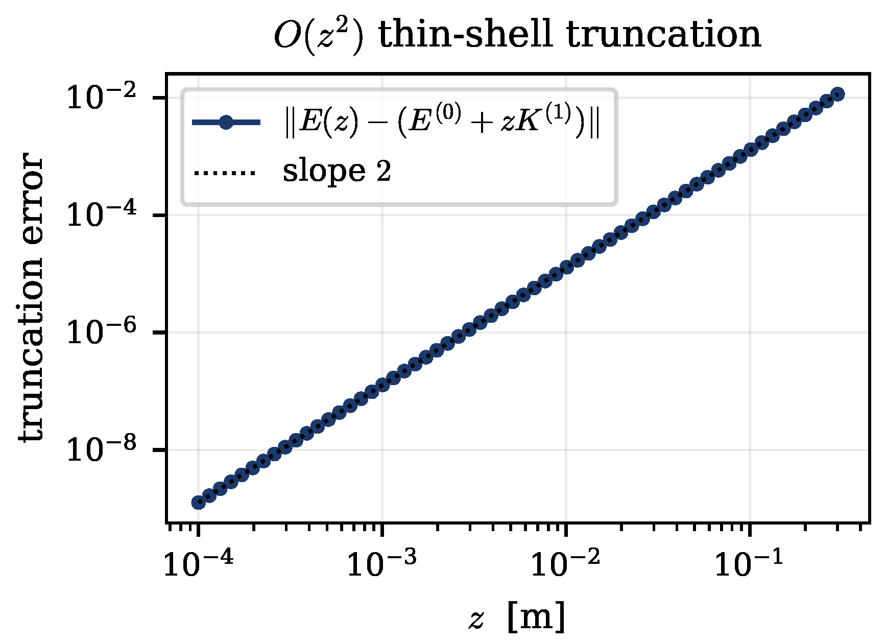
Corollary 1 claims that discarding costs . This is tested on the same patch under a genuine (non-rigid) deformation with a non-symmetric stretch of and a rotation, by comparing the exact from (20) against . Figure 3 confirms the quadratic rate over three decades.
Figure 3.
Thin-shell truncation error against fibre coordinate z, confirming the estimate (21).
Figure 3.
Thin-shell truncation error against fibre coordinate z, confirming the estimate (21).
10.3. Axisymmetric Reduction of the General Theory
For the case study we specialise to shells of revolution undergoing axisymmetric, torsionless deformation. This retains both principal curvatures, non-constant Lamé parameters and non-zero Gaussian curvature, so it exercises the full geometric content of Section 2–Section 5 while reducing the field equations to one spatial dimension.
Let s be reference meridian arclength, the circumferential angle. The reference meridian is with tangent angle ,
One checks immediately that (10) is trivial and (11) reduces to , an identity—an instance of Theorem 1.
The deformed meridian is ; the Kirchhoff–Love constraint means the tangent angle is not independent:
Evaluating Definition 2 in the orthonormal reference coframe gives
Proposition 8
(Axisymmetric strain measures).
Remark 14
(Green–Lagrange versus naive curvature change). Note that and , where and are the true current principal curvatures. The Green–Lagrange bending measure is therefore not but a stretch-weighted version of it; the two differ at relative order . In the small-strain/large-rotation regime typical of thin shells the difference is immaterial, but it is not zero, and using with the energy (51) is variationally inconsistent. The correction is of the same type as the one distinguishing the Budiansky–Sanders “best” first-order theory [6,38] from Love’s, namely a term bilinear in the membrane strain and the second fundamental form; see ([42], Remarks 2.2), who report that the choice makes no significant numerical difference. As a concrete illustration, a sphere of radius inflated uniformly by a stretch λ has even though it remains a sphere.
The stored energy (51) in the thin-shell limit (47) becomes
Loading is a uniform live (follower) pressure, treated exactly through its potential
V being the enclosed volume. Because (62) is an exact potential the problem remains variational at finite deformation, and the tangent operator stays symmetric—a property that pressure loads treated as configuration-independent surface tractions do not possess.
10.4. Discretisation
Since (61) involves second derivatives of , the trial space must be (Remark 4). We use cubic Hermite elements with nodal degrees of freedom and 5-point Gauss–Legendre quadrature. Three implementation choices are worth recording.
- (1)
- Discretely strain-free reference. The reference meridian is interpolated by the same Hermite basis and (60) is evaluated symmetrically in the current and reference fields. The discrete reference state then has exactly zero energy and zero residual (verified: and in double precision), rather than the spurious initial stress produced by comparing an interpolated current state against an exact reference.
- (2)
- Complex-step gradients. Every expression in (60) is complex-analytic—in particular is avoided by carrying directly —— the complex-step derivative [32,46] applies, and the residual is obtained as with , exact to machine precision and free of subtractive cancellation. The tangent (55) follows by central differencing of these gradients; it agrees with a finite-difference tangent of the residual to relative and is exactly symmetric, confirming the variational consistency of Theorem 3.
- (3)
- Path following. Equilibria are traced under apex-deflection control, with the pressure p carried as an extra unknown and the equilibrium equation at the controlled degree of freedom appended, so that limit points in p are passed without difficulty. This is a displacement-controlled variant of the arclength schemes of Wempner [54], Riks [37] and Crisfield [12].
10.5. Verification Against Classical Plate Solutions
The flat-plate specialisation (, ) of (60) is tested against two classical results for a clamped circular plate with immovable edge, radius mm, thickness mm.
In the small-deflection limit the computed centre deflection matches to relative at , drifting to at and at —the departure being physical membrane stiffening, not error. In the large-deflection regime, Table 2 compares against the classical one-term Galerkin result of Timoshenko and Woinowsky-Krieger ([52], Art. 97) .
Figure 4.
Clamped circular plate under uniform pressure. (a) Large-deflection response against Timoshenko’s and the linear solution. (b) Departure of the computed centre deflection from the small-deflection result , showing the onset of membrane stiffening.
Figure 4.
Clamped circular plate under uniform pressure. (a) Large-deflection response against Timoshenko’s and the linear solution. (b) Departure of the computed centre deflection from the small-deflection result , showing the onset of membrane stiffening.
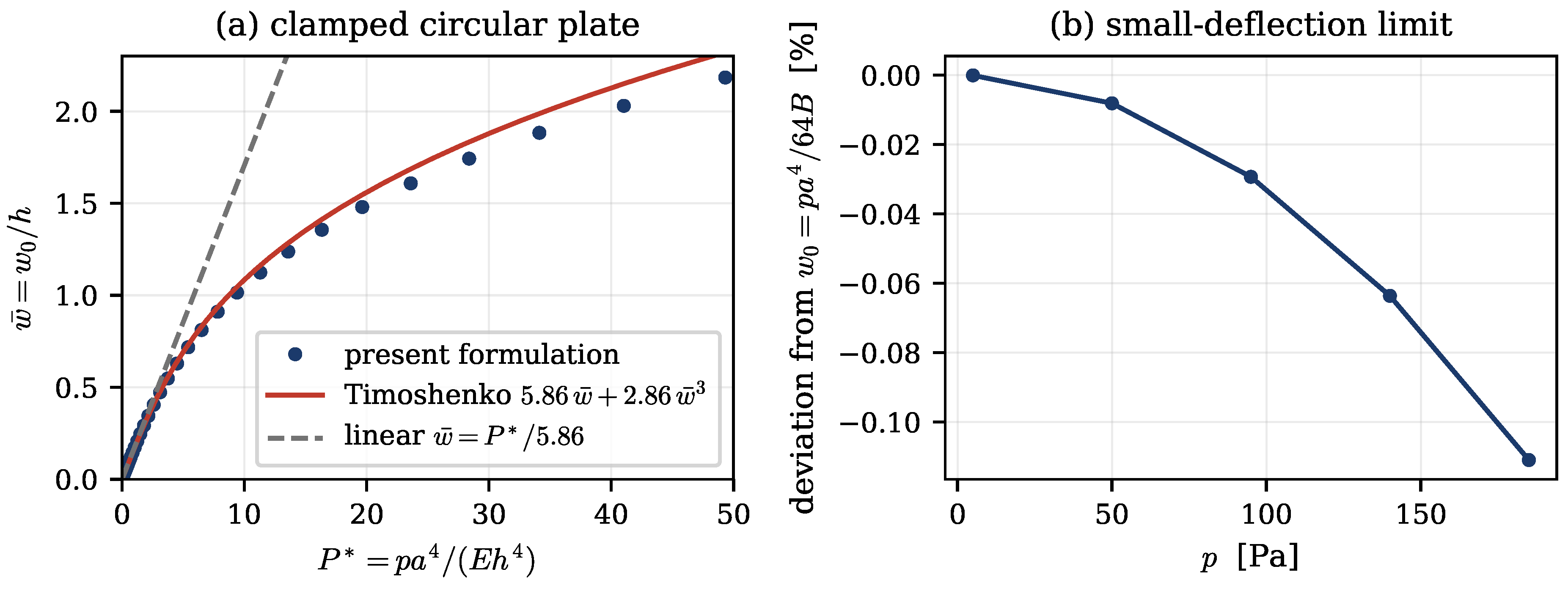
Table 2.
Clamped circular plate, large deflection. . The growing deviation is expected: the reference expression is a one-term Galerkin approximation whose cubic coefficient is known to be low at large , whereas the present computation is a converged solution of the geometrically exact problem.
Table 2.
Clamped circular plate, large deflection. . The growing deviation is expected: the reference expression is a one-term Galerkin approximation whose cubic coefficient is known to be low at large , whereas the present computation is a converged solution of the geometrically exact problem.
| p [Pa] | (present) | (Timoshenko) | deviation | |
|---|---|---|---|---|
| 5.0 | 0.0012 | 0.007 | 0.007 | |
| 140.0 | 0.0341 | 0.200 | 0.200 | |
| 500.0 | 0.1209 | 0.714 | 0.714 | |
| 2619.1 | 0.5477 | 3.742 | 3.679 | |
| 7909.5 | 1.1240 | 11.299 | 10.648 | |
| 19867.9 | 1.7428 | 28.383 | 25.352 | |
| 60000.0 | 2.6949 | 85.714 | 71.769 |
10.6. Comparison with Exact and Published Solutions
The verifications so far are internal. This subsection compares the formulation against three independent reference solutions that it played no part in producing (Figure 5).
Figure 5.
Comparison against exact reference solutions. (a) Axisymmetric free-vibration eigenvalues of a clamped circular plate against the exact Bessel-function values (dashed). (b) Linear deflection profile against Timoshenko and Woinowsky-Krieger’s closed form . (c) Meridional resultant of a clamped spherical cap normalised by the membrane (Young–Laplace) value ; the three pressures collapse onto a single curve, confirming that the interior offset is a linear edge-restraint effect and not a nonlinear artefact.
Figure 5.
Comparison against exact reference solutions. (a) Axisymmetric free-vibration eigenvalues of a clamped circular plate against the exact Bessel-function values (dashed). (b) Linear deflection profile against Timoshenko and Woinowsky-Krieger’s closed form . (c) Meridional resultant of a clamped spherical cap normalised by the membrane (Young–Laplace) value ; the three pressures collapse onto a single curve, confirming that the interior offset is a linear edge-restraint effect and not a nonlinear artefact.
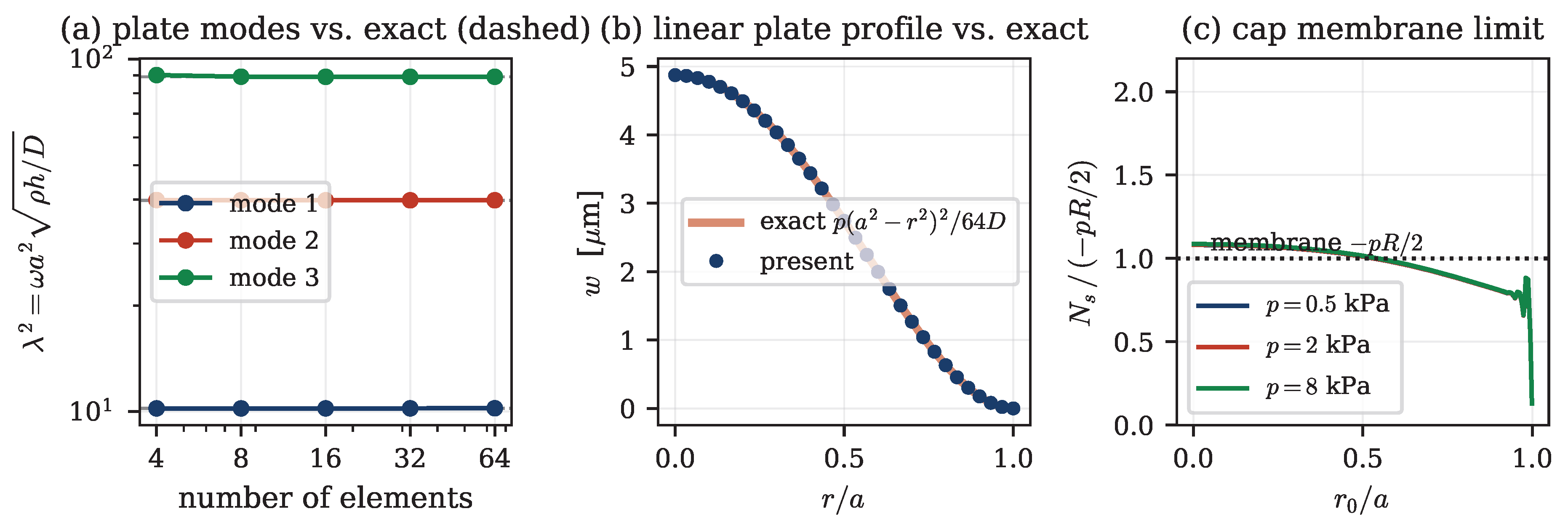
(a) Free vibration of a clamped circular plate.
The axisymmetric natural frequencies satisfy the classical characteristic equation [27,52]
whose first three roots are . Table 3 compares these with the eigenvalues of the discrete pencil at zero load. Four cubic Hermite elements already give the fundamental frequency to . This is the only external validation of the mass matrix and of the tangent operator used for the stability analysis of Section 10.9, and it is therefore the comparison that most directly underwrites Figure 10.
Table 3.
Axisymmetric vibration eigenvalues of a clamped circular plate; relative error against the exact roots of (63) in parentheses. The error passes through a minimum near 16 elements and then grows: beyond that point the accuracy is limited not by the discretisation but by the finite-difference construction of the tangent operator, whose relative error () is amplified by the growing condition number of .
Table 3.
Axisymmetric vibration eigenvalues of a clamped circular plate; relative error against the exact roots of (63) in parentheses. The error passes through a minimum near 16 elements and then grows: beyond that point the accuracy is limited not by the discretisation but by the finite-difference construction of the tangent operator, whose relative error () is amplified by the growing condition number of .
| elements | |||
|---|---|---|---|
| 4 | () | () | () |
| 8 | () | () | () |
| 16 | () | () | () |
| 32 | () | () | () |
| 64 | () | () | () |
| exact |
(b) Linear plate deflection profile.
Beyond the centre deflection of Section 10.5, the whole computed profile is compared against ([52], Art. 62). The two are graphically indistinguishable at Pa; the maximum pointwise deviation is below of the centre deflection. This checks the bending operator and the clamped boundary conditions pointwise rather than at a single functional.
(c) Membrane limit of the spherical cap.
For a spherical shell under uniform pressure, membrane equilibrium (Young–Laplace) gives . Figure 5(c) plots for three pressures spanning a factor of sixteen. The interior value is , and respectively—constant to better than across the load range, and dropping sharply only inside the edge layer of width . The formulation therefore reproduces the membrane state up to a fixed offset attributable to the immovable clamped edge, which for a shallow cap contributes a uniform additional compression that does not decay into the interior. That the offset is independent of p confirms it is a linear edge-restraint effect rather than an error in the pressure functional; the enclosed-volume functional (62) itself reproduces the exact cap volume to 8 significant figures.
Remark 15
(What is not compared). We deliberately do not overlay published critical pressures on Figure 7. The classical axisymmetric results of Budiansky [5] and the bifurcation results of Huang [18] and Weinitschke [53] are reported graphically as against a shallowness parameter whose normalisation differs between authors, and we have not had access to tabulated values. Digitising a published figure and presenting the result as a quantitative comparison would give a false impression of precision. The values in Table 4 should therefore be read as lying within the band those authors report, not as validated against them; the quantitative validations of this paper are those of Sections 10.1, 10.2, 10.5 and 10.6.
10.7. Mesh Convergence
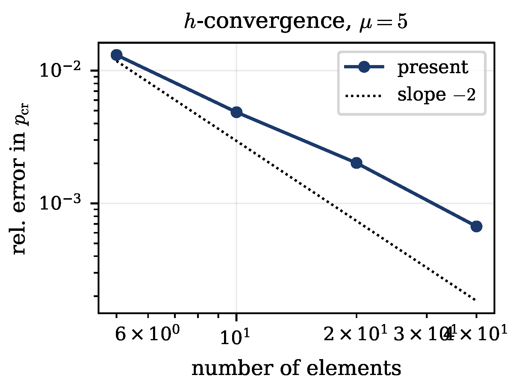
Figure 6 shows h-convergence of the critical snap-through pressure for the cap of Section 10.8. The computed values are for elements. Even five cubic Hermite elements are within ; the observed rate is consistent with the expected for a limit-point load computed from a cubic discretisation. All subsequent results use 30 elements.
Figure 6.
Mesh convergence of the critical pressure, cap; the 80-element value is taken as reference.
Figure 6.
Mesh convergence of the critical pressure, cap; the 80-element value is taken as reference.
10.8. Snap-Through of Clamped Spherical Caps
We now apply the formulation to its intended regime. A clamped spherical cap of sphere radius m and thickness mm is loaded by uniform external pressure. Cap geometry is parameterised by the shallowness number of Budiansky [5] and Huang [18],
H being the rise; pressures are normalised by the classical buckling pressure of a complete sphere, kPa, the Zoelly result [55]. Three caps are considered, listed in Table 4.
Table 4.
Cap geometries and computed critical loads. is the upper limit point, the following minimum (the lower limit point). The cap is too shallow to lose stability: its equilibrium path is monotone and its fundamental frequency never vanishes.
Table 4.
Cap geometries and computed critical loads. is the upper limit point, the following minimum (the lower limit point). The cap is too shallow to lose stability: its equilibrium path is monotone and its fundamental frequency never vanishes.
| base radius a [mm] | at [Hz] | |||||
|---|---|---|---|---|---|---|
| 3 | 1.36 | 73.8 | —(monotone) | — | — | 1462.9 |
| 4 | 2.42 | 98.3 | 0.5648 | 1.01 | 0.4247 | 1237.5 |
| 5 | 3.78 | 122.8 | 0.6168 | 0.83 | 0.2846 | 1139.4 |
Figure 7 shows the complete equilibrium paths. The transition between monotone and snapping behaviour occurs between and , consistent with the classical picture [5,18,22,53]. The critical pressures, and times , lie in the band reported for clamped shallow caps in the axisymmetric analyses of [5,7], though see Remark 15 on the limits of that statement and Section 10.13(ii) on axisymmetry.
Figure 8 makes the mechanism visible: the apex displacement at state F exceeds , so the shell has passed entirely through its own base plane. Rotations of the meridian normal exceed over much of the cap. This is precisely the regime in which the spurious strain of Figure 2 would dominate a linearised formulation.
Figure 9 isolates the term identified in Remark 8. At the limit point the meridional resultant is compressive over the whole cap, and the geometric-stiffness density is large and negative near the clamped edge, where the bending boundary layer of width mm concentrates the curvature change. Omitting this term—or replacing by N — changes the computed critical pressure and destroys the correspondence between limit points and vanishing frequencies established next.
Figure 7.
Equilibrium paths of clamped spherical caps under uniform pressure. Downward triangles mark upper limit points, upward triangles the following minima. The cap stiffens monotonically; and 5 exhibit classical snap-through, the unstable segment between the two limit points being traversable only under displacement control.
Figure 7.
Equilibrium paths of clamped spherical caps under uniform pressure. Downward triangles mark upper limit points, upward triangles the following minima. The cap stiffens monotonically; and 5 exhibit classical snap-through, the unstable segment between the two limit points being traversable only under displacement control.
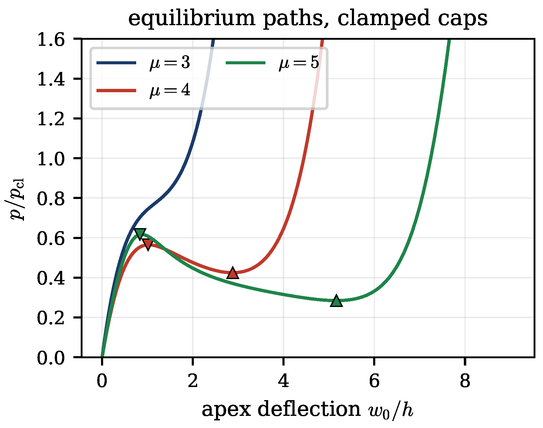
Figure 8.
Deformation sequence for the cap. (a) Meridian profiles at the six marked states; the cap passes continuously from the initial convex shape (A) through the limit point (B) and the unstable branch (C, D) to a fully inverted, re-stiffening configuration (F). (b) Location of each state on the equilibrium path.
Figure 8.
Deformation sequence for the cap. (a) Meridian profiles at the six marked states; the cap passes continuously from the initial convex shape (A) through the limit point (B) and the unstable branch (C, D) to a fully inverted, re-stiffening configuration (F). (b) Location of each state on the equilibrium path.
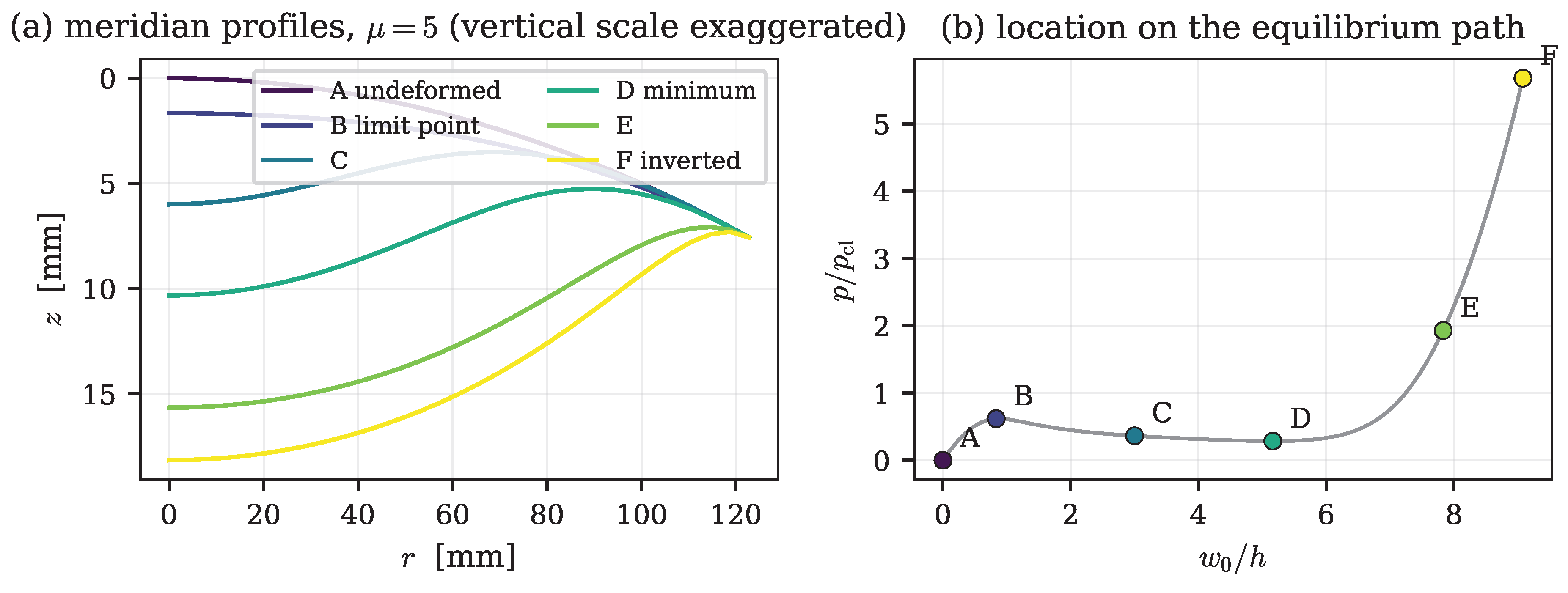
Figure 9.
Stress resultants and geometric-stiffness density for the cap at the limit point (B), the minimum (D) and the fully inverted state (F). Solid lines: meridional; dashed: circumferential. The right panel shows of (40), the term responsible for the instability.
Figure 9.
Stress resultants and geometric-stiffness density for the cap at the limit point (B), the minimum (D) and the fully inverted state (F). Solid lines: meridional; dashed: circumferential. The right panel shows of (40), the term responsible for the instability.
10.9. Dynamic Signature of the Instability
Because the formulation is variational, the second variation (55) evaluated at an equilibrium is the tangent stiffness of the linearised dynamics, and the generalised eigenproblem —with the consistent mass matrix from (35)—gives the natural frequencies of small vibration about that state. Stability and dynamics are therefore not separate calculations.
Figure 10(a) is the sharpest available check on the internal consistency of the whole formulation. The frequency computed from crosses zero at and for , and at and for ; the limit points located independently from the load–deflection curve are at and , and and . The two determinations agree to the resolution of the path discretisation, as they must if the tangent operator is genuinely the second variation of the same energy whose stationarity defines the path. For the frequency dips but never reaches zero, in agreement with the monotone path.
Figure 10.
(a) Fundamental frequency along the equilibrium paths, plotted with the sign of the corresponding eigenvalue of : it passes through zero exactly at the limit points (triangles) and is imaginary (plotted negative) on the unstable branch. The cap never loses positive-definiteness. (b) Southwell-type frequency–load relation for : is close to linear in at low load and departs as the limit point is approached.
Figure 10.
(a) Fundamental frequency along the equilibrium paths, plotted with the sign of the corresponding eigenvalue of : it passes through zero exactly at the limit points (triangles) and is imaginary (plotted negative) on the unstable branch. The cap never loses positive-definiteness. (b) Southwell-type frequency–load relation for : is close to linear in at low load and departs as the limit point is approached.
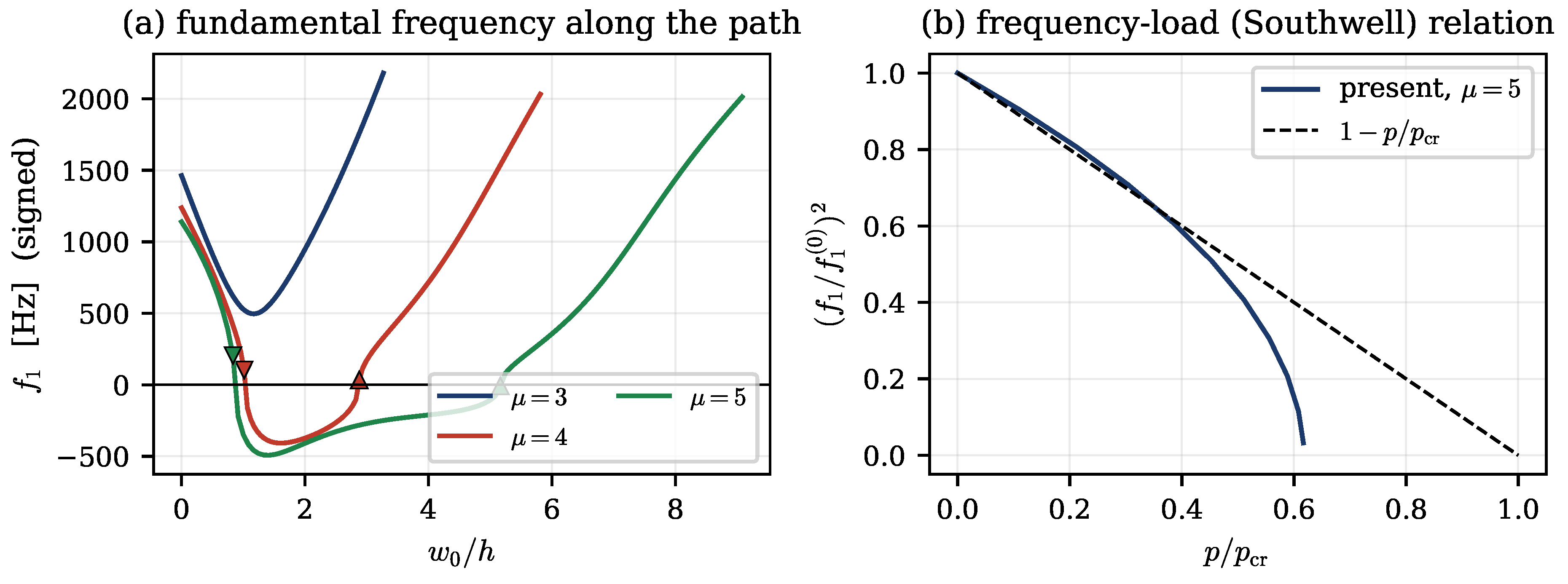
Panel (b) shows the frequency–load relation used in non-destructive buckling estimation. The near-linearity of against at low load is the Southwell/Lurie behaviour that underwrites vibration-based load estimation; the pronounced departure above quantifies the error incurred by extrapolating it, which for this cap would over-predict the critical pressure by about .
10.10. Comparison with Published Finite-Element Results
The comparisons of Section 10.6 are against closed-form solutions. This subsection compares against published numerical results obtained with entirely different shell formulations. We use the benchmark suite of Simo, Fox and Rifai [43], which reports tabulated values—not only figures—and which was explicitly documented by its authors to promote comparison with other formulations.
Roll-up of a clamped strip ([43], Section 6.1.1).
An initially flat strip (, , , , ) under an end moment rolls into a complete circle of radius . Evaluating Definition 2 on the exact rolled-up configuration gives — the deformation is recognised as an exact isometry—and against the exact . The residual is the finite-difference error of the surface derivatives used in this particular check, not of the theory. This is the shell-theoretic content of the benchmark: a rotation with identically zero membrane strain. In [43] the complete roll-up is driven in a single load step on a 25-element mesh, which is the practical demonstration that the director parametrisation is singularity-free; the check performed here is of the strain measures alone and involves no incremental solution.
Between them the companion papers report a much larger suite. Part II ([42], Sections 7.1–7.8) covers the linear tests—constant tension, bending and in-plane twist patch tests on regular and skewed meshes, Cook’s membrane, the singularity-dominated rhombic plate, the twisted ribbon, the pinched hemisphere both with an hole and closed, the Scordellis–Lo barrel vault, the pinched cylinder with end diaphragms, and two mesh-distortion studies (a simply supported plate distorted to the point of a negative Jacobian, and a cantilever of ten arbitrarily skewed elements)—while Part III adds the nonlinear ones: in-plane bending on a deliberately distorted mesh, torsion of a flat strip through , the finite-strain pinched hemisphere, buckling of a simply-supported plate, an L-shaped frame, and snap-through of a hinged cylindrical panel ([43], Sections 6.1–6.3). None of these is axisymmetric—in the Part II suite the hemisphere is the only axisymmetric geometry, and its loading, four alternating point forces at , is not — so none is accessible to the reduction of Section 10.3, and we make no comparison against them. Part II does tabulate its results ([42], Tables 9–17) rather than reporting them graphically, so the obstacle is the kinematics of the benchmarks and not the availability of numbers.
One benchmark in Part III is an exception worth recording. The collapse of a clamped rubber sphere under a point load ([43], Section 6.3.3) is axisymmetric, and [43] compute it with transverse shear suppressed by a penalty precisely in order to match the shear-rigid theory of Taber [50], against which experimental data are reported. It is therefore a rare instance of a published, experimentally anchored, shear-rigid, axisymmetric, large-deflection benchmark—a natural target for the present formulation. We have not attempted it, because with and it lies well outside the thin, small-strain regime in which the Saint-Venant–Kirchhoff closure of Section 7 is defensible (Section 10.13(iii)). We flag it as the obvious next validation step. Table 2 of [42] is used separately in Section 7.2.
Axially compressed clamped cylinder ([43], Table 6.2.3).
A cylinder with , , , , (, ) is compressed axially between clamped ends. Simo et al. report that for clamped ends the critical mode is axisymmetric, which is what makes this benchmark accessible to the present axisymmetric reduction. Loads are normalised by ([51], p. 465).
Following [43] we perform a linearised buckling analysis: the material stiffness and the geometric stiffness are extracted from the tangent operator at imposed end shortening , and the eigenproblem is solved. Table 5 and Figure 11 give the result.
Figure 11.
Comparison with ([43], Table 6.2.3) for the clamped axially compressed cylinder. (a) The present value lies within the spread of the three published formulations. (b) Mesh convergence: the present value is converged to four figures from 40 elements onwards. (c) The computed critical mode is the axisymmetric ring-wave pattern reported in ([43], Figure 6.2.4(b)).
Figure 11.
Comparison with ([43], Table 6.2.3) for the clamped axially compressed cylinder. (a) The present value lies within the spread of the three published formulations. (b) Mesh convergence: the present value is converged to four figures from 40 elements onwards. (c) The computed critical mode is the axisymmetric ring-wave pattern reported in ([43], Figure 6.2.4(b)).
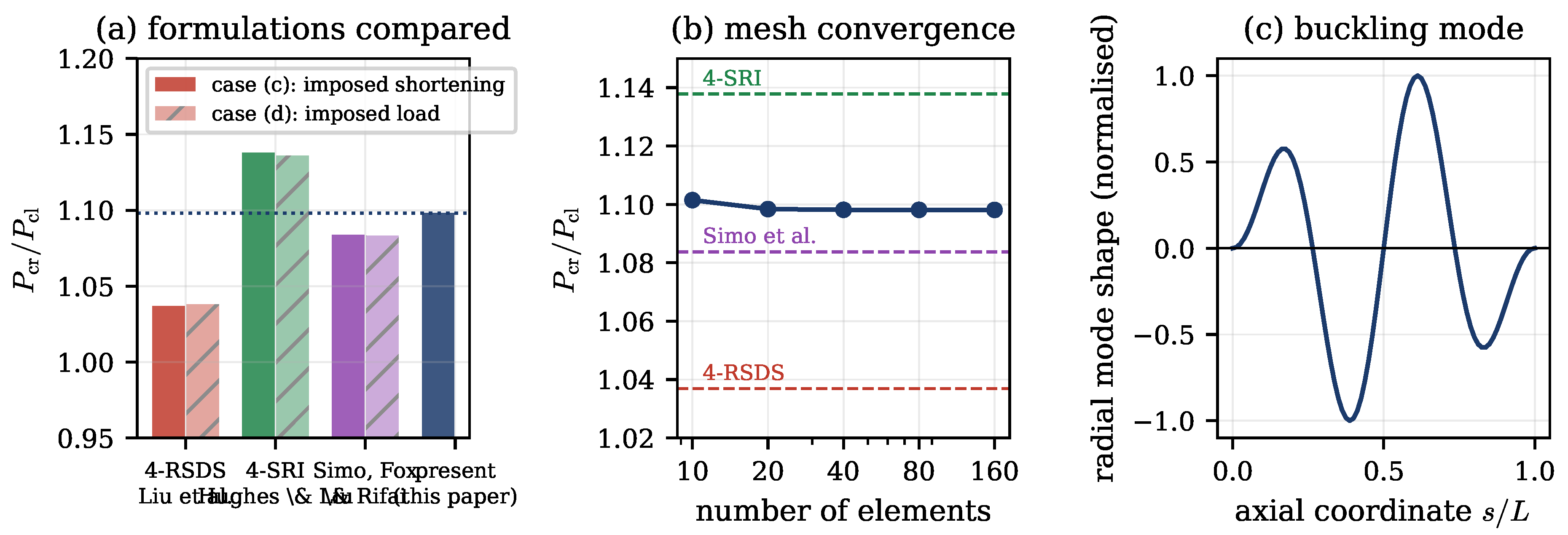
Table 5.
Normalised critical load for the clamped axially compressed cylinder of ([43], Table 6.2.3). Case (c): imposed end shortening; case (d): imposed compressive load. Reference values are quoted directly from ([43], Table 6.2.3); 4-RSDS is the resultant-stress degenerated element of Liu et al. [29] and 4-SRI the selectively-integrated degenerated element of Hughes and Liu [21].
Table 5.
Normalised critical load for the clamped axially compressed cylinder of ([43], Table 6.2.3). Case (c): imposed end shortening; case (d): imposed compressive load. Reference values are quoted directly from ([43], Table 6.2.3); 4-RSDS is the resultant-stress degenerated element of Liu et al. [29] and 4-SRI the selectively-integrated degenerated element of Hughes and Liu [21].
| Formulation | kinematics | case (c) | case (d) |
|---|---|---|---|
| 4-RSDS [29] | degenerated solid, shear-flexible | ||
| 4-SRI [21] | degenerated solid, shear-flexible | ||
| Simo, Fox & Rifai [43] | one-director Cosserat, shear-flexible | ||
| present | Kirchhoff–Love, shear-rigid | — |
The present value differs from Simo et al. by , lies below 4-SRI and above 4-RSDS—that is, comfortably inside the spread of the three published results, and closest to the geometrically exact formulation of the three. Two remarks are in order.
- (i)
- The residual against [43] has an identifiable origin: the present theory is Kirchhoff–Love and therefore shear-rigid, whereas all three reference formulations admit transverse shear. A shear-rigid model is stiffer and must over-predict the buckling load; the sign of the discrepancy is therefore the expected one, and its magnitude is consistent with where is the axial buckle half-wavelength.
- (ii)
- We compare only case (c). Cases (a) and (b) of ([43], Table 6.2.3) have free ends, for which the reported critical loads fall to and —about half the clamped value, in agreement with the analytical result of Hoff and Soong [17]—in a mode carrying two circumferential sine-waves and none in the axial direction. That mode is non-axisymmetric and therefore outside the reach of the present reduction (Section 10.13(ii)). We do not report a value for it.
- (iii)
- The axisymmetry of the mode is a property of the linearised analysis, not of the structure. When the eigenvalue problem is re-solved at the computed bifurcation point instead of at the reference configuration, the clamped cylinder’s critical mode is no longer axisymmetric but reticulated, at ([43], Section 6.2.4). What Table 5 compares is thus the linearised buckling load as computed by four formulations under one and the same restrictive assumption, not the true critical load of the cylinder. Simo et al. draw the explicit moral that linearised buckling results “should be interpreted with caution”; we adopt it. The same caveat attaches to the caps of Section 10.8—see Section 10.13(ii).
10.11. Asymptotic Convergence of the Newton Iteration
Remark 13 claims that the tangent used here is the exact derivative of the discrete residual. That claim has an observable consequence, and it is the sharpest single test of a nonlinear implementation available: an exact tangent forces the Newton error to contract quadratically, and nothing else does. Simo, Fox and Rifai report this rate for their formulation in ([43], Tables 6.4.1–6.4.3), which makes it directly comparable.
We take one large load step from the undeformed state and iterate with undamped Newton—no line search, no step limiting—recording the Euclidean norm of the out-of-balance force and the energy norm . Table 6 gives the two sequences and Figure 12 plots them.
The energy norm falls by eighteen decades in eight iterations for the plate and by twenty-one in five for the cap. Fitting over the asymptotic range gives – in both cases, and Figure 12(b) shows the points lying on the slope-2 reference line rather than the slope-1 line that an approximate tangent would produce. The behaviour matches that of ([43], Tables 6.4.1–6.4.3) closely enough that the two sets of sequences are hard to separate in Figure 12(a), which is the expected outcome: quadratic convergence is a property of exact linearisation, not of a particular shell theory, and its appearance in both is evidence that both linearisations are in fact exact.
Table 6.
Newton convergence in a single load step with the consistent tangent. Left: clamped circular plate (30 elements) at Pa, i.e., apex deflection , deep in the nonlinear regime. Right: clamped spherical cap (, 30 elements) at . Both bottom out at the round-off floor of the residual evaluation, in the units of the problem.
Table 6.
Newton convergence in a single load step with the consistent tangent. Left: clamped circular plate (30 elements) at Pa, i.e., apex deflection , deep in the nonlinear regime. Right: clamped spherical cap (, 30 elements) at . Both bottom out at the round-off floor of the residual evaluation, in the units of the problem.
| clamped plate | spherical cap | ||||
|---|---|---|---|---|---|
| k | k | ||||
| 0 | 0 | ||||
| 1 | 1 | ||||
| 2 | 2 | ||||
| 3 | 3 | ||||
| 4 | 4 | ||||
| 5 | 5 | ||||
| 6 | |||||
| 7 | |||||
| 8 | |||||
Figure 12.
Asymptotic convergence of the Newton iteration with the consistent tangent. (a) Energy norm against iteration number, normalised by its value at ; the dashed curves are the corresponding sequences reported by Simo, Fox and Rifai ([43], Tables 6.4.1–6.4.3), normalised the same way. (b) The same data as against : a quadratically convergent method must fall on a line of slope 2, a method with an inexact tangent on a line of slope 1. The present sequences track slope 2 until the round-off floor of the residual evaluation is reached.
Figure 12.
Asymptotic convergence of the Newton iteration with the consistent tangent. (a) Energy norm against iteration number, normalised by its value at ; the dashed curves are the corresponding sequences reported by Simo, Fox and Rifai ([43], Tables 6.4.1–6.4.3), normalised the same way. (b) The same data as against : a quadratically convergent method must fall on a line of slope 2, a method with an inexact tangent on a line of slope 1. The present sequences track slope 2 until the round-off floor of the residual evaluation is reached.
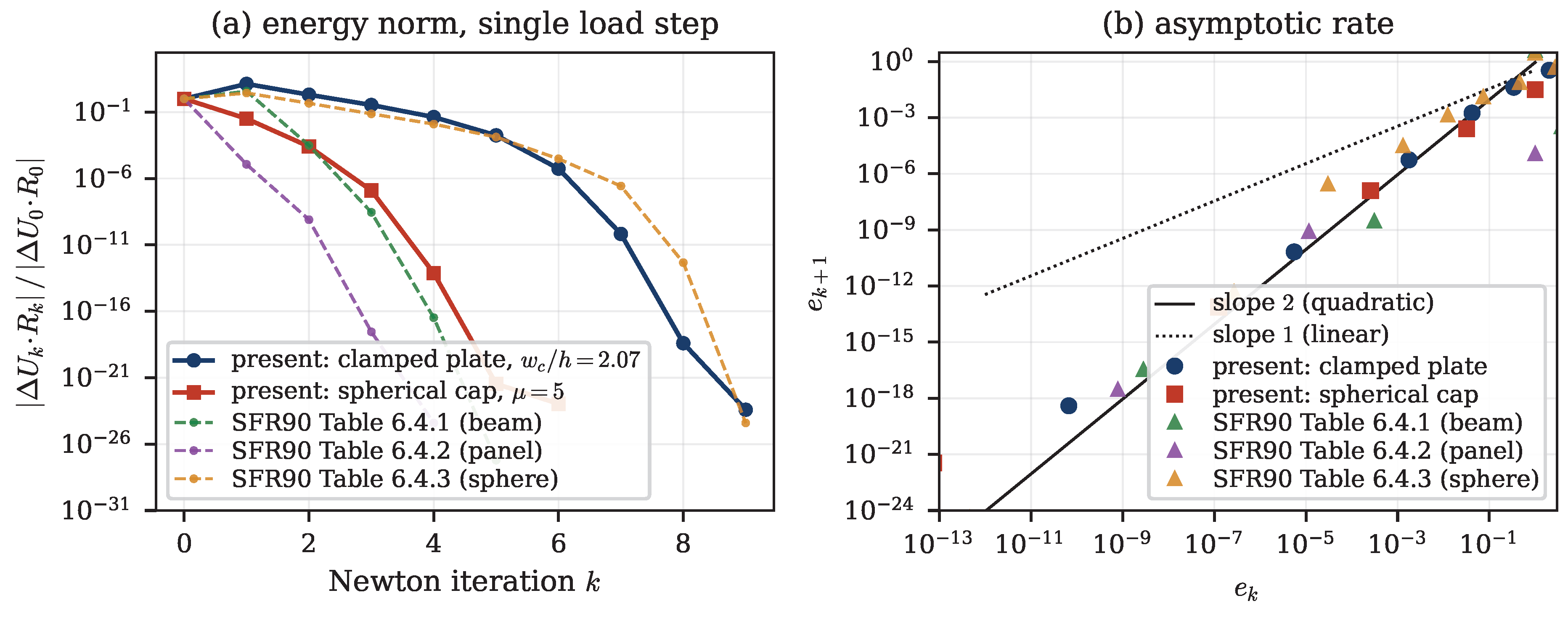
Two caveats. First, the first one or two iterations are not in the asymptotic regime and need not contract at all—the plate residual rises by two orders of magnitude at , and the same non-monotonicity is visible in ([43], Table 6.4.3), where the residual rises at the first iteration of a one-step collapse computation. Quadratic convergence is an asymptotic statement and nothing more. Second, undamped Newton from an undeformed state has a finite basin: at the cap iteration diverges, and the damped scheme used for the production runs of Section 10.8 is required. This is a property of Newton’s method, not of the tangent.
10.12. Summary of Verification
Table 7 collects every quantitative check performed, with its reference solution and source. The distinction between the three columns matters: exact references are closed-form or machine-computable to arbitrary precision; published references are approximate solutions from the literature, so a discrepancy does not by itself indicate an error in the present work; internal checks test consistency between parts of this paper and cannot detect an error common to both.
Table 7.
Complete verification record. “E” = exact reference, “P” = published approximate reference, “I” = internal consistency check.
Table 7.
Complete verification record. “E” = exact reference, “P” = published approximate reference, “I” = internal consistency check.
| Quantity | Reference | Agreement | |
|---|---|---|---|
| Strain under finite rigid rotation | , Theorem 2 | E | –, all |
| Thickness truncation | , Corollary 1 | E | measured slope |
| Discrete reference state | zero energy, zero residual | E | (exact, double precision) |
| Plate centre deflection, small p | ([52], Art. 62) | E | relative |
| Plate deflection profile | [52] | E | pointwise |
| Plate vibration | , roots of (63) [27] | E | with 4 elements |
| Plate vibration | , [27] | E | , (16 el.) |
| Cap enclosed volume | E | 8 significant figures | |
| Cap interior resultant | (Young–Laplace) | E | – over load range |
| Plate large deflection, | ([52], Art. 97) | P | – |
| Plate large deflection, | as above | P | – (reference is a one-term Galerkin approximation) |
| Cap | [5,18,53] | P | not compared—see Remark 15 |
| Strip roll-up, | , ([43], Section 6.1.1) | E | ; rel. |
| Higher-order stiffness | ([42], Table 2) | P | structure recovered (hyperelastic, same dependence); coupling differs by after conversion to bare resultants —Remark 11 |
| Cylinder | ([43], Table 6.2.3) | P | (); within the spread of three published formulations |
| Tangent operator | finite difference of the residual | I | ; exactly symmetric |
| Newton asymptotic rate | 2, as for any exact tangent; cf. ([43], Tables 6.4.1–6.4.3) | I | measured – over decades |
| Limit points vs. | must coincide if variational | I | agree to path resolution |
| Mesh convergence of | 80-element value | I | with 5 elements |
Remark 16
(On what the reader should conclude). The exact checks establish that the kinematics, the bending operator, the mass matrix, the pressure functional and the tangent operator are all correct, in the strong sense that each reproduces an independently known answer to several significant figures. What they do not establish is that the snap-through pressures of Table 4 agree with the literature, because we have not been able to make that comparison quantitatively (Remark 15). A reader who needs those numbers for design purposes should treat them as the output of a verified code applied to a problem whose published solutions we could not access in tabulated form, and not as validated predictions.
10.13. Limitations
Three restrictions of the case study should be stated plainly.
- (i)
- Deeper caps. For the axisymmetric equilibrium branch develops a fold in the apex deflection and in the enclosed volume near the upper limit point, so that neither load, apex-displacement nor volume control is a globally valid parameterisation. Tracing those branches requires true arclength continuation with adaptive step control. We have therefore restricted the reported results to , where the paths are traversed without a single failed increment.
- (ii)
- Axisymmetry. The computation constrains deformation to be axisymmetric. Real spherical caps frequently buckle first into a non-axisymmetric mode [18,20,53], so the loads in Table 4 are upper bounds on the true critical pressures. Detecting those modes requires a Fourier decomposition in and a bifurcation check on each harmonic; the theory of Section 2–Section 9 supports this without modification, but the implementation does not. The restriction is not peculiar to caps: the axially compressed cylinder of Section 10.10 behaves the same way, its linearised clamped mode being axisymmetric while the mode computed at the bifurcation point is not ([43], Section 6.2.4).
- (iii)
- Constitutive scope. A Saint-Venant–Kirchhoff law is used, which is appropriate for the small-strain/large-rotation regime of these examples () but is not a sound finite-strain model. Nothing in Section 2–Section 5 depends on this choice; only (45) and (51) would change; see [2,47] for finite-strain shell constitutive theory.
11. Conclusions
Treating the shell body as a fibre bundle and its geometry through a moving coframe is not a change of notation. It changes what has to be assumed and what follows.
- Compatibility becomes an identity. The Gauss and Codazzi–Mainardi equations are the components of the curvature 2-form , which vanishes because the reference configuration is embedded in flat space (Theorem 1). They need not be imposed or verified.
- Objectivity becomes exact. Because the strain measures are differences of pulled-back metrics, invariance under is an algebraic identity (Theorem 2), confirmed numerically at the level over the full range of rotation angles. Table 1 quantifies what is lost otherwise: MPa of fictitious stress at .
- Dimensional reduction becomes fibre integration. Carrying the exact shifter determinant through the fibre integral yields resultant stiffnesses (34) including a curvature-induced membrane–bending coupling that the usual derivation discards without comment.
- The balance laws acquire their missing terms. Deriving Theorem 3 from the variational statement rather than by analogy exposes the effective resultant , the shear–curvature coupling in the tangential equation, and the Kirchhoff corner forces (43). Figure 9 shows that the geometric-stiffness density is precisely the instability mechanism.
- Stability and dynamics coincide. Because the theory is variational, the tangent operator is the second variation, and the vanishing of the fundamental frequency at the limit points (Figure 10) is automatic rather than coincidental. This is the strongest single check on the consistency of the formulation, and it is passed to the resolution of the path discretisation.
A further caveat deserves emphasis: the loads computed here are those of the perfect shell. Spherical shells are notoriously imperfection-sensitive [7,20,22], and experimentally observed buckling pressures fall well below the perfect-shell values. The present formulation is well suited to imperfection studies, since an imperfect reference surface enters only through and requires no change to any equation.
The natural continuations are non-axisymmetric bifurcation analysis via harmonic decomposition, finite-strain constitutive laws (for which only Section 7 changes), and isogeometric discretisation [19,23], which supplies the regularity that Remark 4 shows to be intrinsic to the Kirchhoff–Love constraint rather than a numerical convenience.
Author Contributions
Bo Hua Sun: Conceptualization, Methodology, Formulations, Formal analysis, Funding acquisition, Investigation, Writing- Original draft preparation, Writing- Reviewing and Editing and all relevant works.
Data Availability Statement
The data supporting the findings of this study are available from the corresponding author upon reasonable request.
Acknowledgments
My research into shell theory started at Lanzhou University and Ruhr-Universität Bochum, with core work completed during my tenure as a professor at the Cape Peninsula University of Technology (CPUT), South Africa. I am profoundly grateful to CPUT for granting me the unrestricted academic autonomy to pursue this research agenda–this vital institutional support laid the groundwork for the principal conclusions presented in this manuscript. I extend my most sincere thanks to former Vice-Chancellor (now Chancellor) Prof. Brian Figaji, as well as former Deputy Vice-Chancellors Prof. J. A. Tromp and Prof. Anthony Staak, for their generous endorsement. Further academic support was provided by Jian University (JNU), Xi’an University of Architecture and Technology (XAUAT) and the Beijing Institute of Nanoenergy and Nanosystems (BINN), Chinese Academy of Sciences. I sincerely thank former JNU President Renhuai Liu, XAUAT President Prof. Xiao-Jun Liu and current President Prof. Xiang-Mo Zhao, along with BINN Founding Director Prof. Zhong Lin Wang, for their unwavering encouragement and invaluable resource support throughout this study.
Conflicts of Interest
The authors declare that there are no competing financial interests.
Appendix A. Summary of Corrections
For convenience, the errors discussed in the text are collected here.
Table A1.
Frequently encountered errors in Kirchhoff–Love shell formulations and their corrections.
| Item | Incorrect form | Correct form (this paper) |
|---|---|---|
| Resultant constitutive law | with and | (46): |
| Bending-strain variation | (26): | |
| Status of the director | “independent variable subject to ” | Remark 4: either constrained () or mixed with multipliers |
| Tangential balance | (39), with and | |
| Curvature sign convention | together with | Remark 2: single convention throughout |
| Boundary conditions | four independent edge conditions | Proposition 6: three, plus corner forces |
| Fibre integration weight | (7), (33): | |
| Consistency at | retaining but dropping | (50): retain both, cf. ([42], Table 2) |
| Effective vs. bare resultants | comparing with directly | (49): convert through first |
References
- Ahmad, S.; Irons, B. M.; Zienkiewicz, O. C. Analysis of thick and thin shell structures by curved finite elements. Int. J. Numer. Methods Eng. 1970, 2, 419–451. [Google Scholar] [CrossRef]
- Antman, S. S. Nonlinear Problems of Elasticity, 2nd ed.; Springer: New York, 2005. [Google Scholar]
- Bathe, K.-J. Finite Element Procedures, 2nd ed.; Prentice-Hall / K.-J. Bathe: Watertown MA, 2014. [Google Scholar]
- Bischoff, M.; Ramm, E.; Irslinger, J. Models and finite elements for thin-walled structures. In Encyclopedia of Computational Mechanics, 2nd ed.; Wiley, 2017. [Google Scholar]
- Budiansky, B. Buckling of clamped shallow spherical shells. In Proc. IUTAM Symposium on the Theory of Thin Elastic Shells, Delft 1959; North-Holland, Amsterdam, 1960; (Also Harvard University Tech. Rep. TR-5, 1959). [Google Scholar]
- Budiansky, B.; Sanders, J. L., Jr. On the “best” first-order linear shell theory. Prog. Appl. Mech. (Prager Anniversary Volume) 1963, 20, 129–140. [Google Scholar]
- Bushnell, D. Computerized Buckling Analysis of Shells; Martinus Nijhoff: Dordrecht, 1985. [Google Scholar]
- Carroll, M. M.; Naghdi, P. M. The influence of the reference geometry on the response of elastic shells. Arch. Ration. Mech. Anal. 1972, 48, 302–318. [Google Scholar] [CrossRef]
- Ciarlet, P. G. An introduction to differential geometry with applications to elasticity. J. Elast. 2005, 78–79, 1–215. [Google Scholar] [CrossRef]
- Cirak, F.; Ortiz, M.; Schröder, P. Subdivision surfaces: A new paradigm for thin-shell finite-element analysis. Int. J. Numer. Methods Eng. 2000, 47, 2039–2072. [Google Scholar] [CrossRef]
- Cirak, F.; Ortiz, M. Fully C1-conforming subdivision elements for finite deformation thin-shell analysis. Int. J. Numer. Methods Eng. 2001, 51, 813–833. [Google Scholar] [CrossRef]
- Crisfield, M. A. A fast incremental/iterative solution procedure that handles “snap-through”. Comput. Struct. 1981, 13, 55–62. [Google Scholar] [CrossRef]
- do Carmo, M. P. Differential Geometry of Curves and Surfaces; Prentice-Hall: Englewood Cliffs NJ, 1976. [Google Scholar]
- Flanders, H. Differential Forms with Applications to the Physical Sciences; Dover, New York, 1989; (Originally Academic Press, 1963). [Google Scholar]
- Fox, D. D.; Raoult, A.; Simo, J. C. A justification of nonlinear properly invariant plate theories. Arch. Ration. Mech. Anal. 1993, 124, 157–199. [Google Scholar] [CrossRef]
- Green, A. E.; Zerna, W. Theoretical Elasticity, 2nd ed.; Oxford University Press: Oxford, 1968. [Google Scholar]
- Hoff, N. J.; Soong, T. C. Buckling of circular cylindrical shells in axial compression. Int. J. Mech. Sci. 1965, 7, 489–520. [Google Scholar] [CrossRef]
- Huang, N.-C. Unsymmetrical buckling of thin shallow spherical shells. ASME J. Appl. Mech. 1964, 31(3), 447–457. [Google Scholar] [CrossRef]
- Hughes, T. J. R.; Cottrell, J. A.; Bazilevs, Y. Isogeometric analysis: CAD, finite elements, NURBS, exact geometry and mesh refinement. Comput. Methods Appl. Mech. Eng. 2005, 194, 4135–4195. [Google Scholar] [CrossRef]
- Hutchinson, J. W. Imperfection sensitivity of externally pressurized spherical shells. ASME J. Appl. Mech. 1967, 34(1), 49–55. [Google Scholar] [CrossRef]
- Hughes, T. J. R.; Liu, W. K. Nonlinear finite element analysis of shells: Part I. Three-dimensional shells. Comput. Methods Appl. Mech. Eng. 1981, 26, 331–362. [Google Scholar] [CrossRef]
- Kaplan, A. Buckling of spherical shells. In Thin-Shell Structures: Theory, Experiment and Design; Fung, Y. C., Sechler, E. E., Eds.; Prentice-Hall: Englewood Cliffs NJ, 1974; pp. 248–288. [Google Scholar]
- Kiendl, J.; Bletzinger, K.-U.; Linhard, J.; Wüchner, R. Isogeometric shell analysis with Kirchhoff–Love elements. Comput. Methods Appl. Mech. Eng. 2009, 198, 3902–3914. [Google Scholar] [CrossRef]
- Kobayashi, S.; Nomizu, K. Foundations of Differential Geometry, Volume I; Interscience: New York, 1963. [Google Scholar]
- Koiter, W. T. On the nonlinear theory of thin elastic shells. Proc. Koninklijke Nederlandse Akademie van Wetenschappen Series B. 1966, 69, 1–54. [Google Scholar]
- Koiter, W. T. On the foundations of the linear theory of thin elastic shells. Proc. K. Ned. Akad. Van. Wet.>, Ser. B 1970, 73, 169–195. [Google Scholar]
- Leissa, A. W. Vibration of Plates; NASA SP-160; U.S. Government Printing Office: Washington DC, 1969.
- Libai, A.; Simmonds, J. G. The Nonlinear Theory of Elastic Shells, 2nd ed.; Cambridge University Press: Cambridge, 1998. [Google Scholar]
- Liu, W. K.; Law, E. S.; Lam, D.; Belytschko, T. Resultant-stress degenerated-shell element. Comput. Methods Appl. Mech. Eng. 1986, 55, 259–300. [Google Scholar] [CrossRef]
- Love, A. E. H. A Treatise on the Mathematical Theory of Elasticity, 4th ed.; Cambridge University Press: Cambridge, 1927. [Google Scholar]
- Makowski, J.; Pietraszkiewicz, W. Work-conjugate boundary conditions in the nonlinear theory of thin shells. ASME J. Appl. Mech. 1989, 56(2), 395–402. [Google Scholar] [CrossRef]
- Martins, J. R. R. A.; Sturdza, P.; Alonso, J. J. The complex-step derivative approximation. ACM Trans. Math. Softw. 2003, 29(3), 245–262. [Google Scholar] [CrossRef]
- Marsden, J. E.; Hughes, T. J. R. Mathematical Foundations of Elasticity; Dover, New York, 1994; (Originally Prentice-Hall, 1983). [Google Scholar]
- Naghdi, P. M. The theory of shells and plates. In Handbuch der Physik; Springer: Berlin, 1972; Volume VIa/2, pp. pages 425–640. [Google Scholar]
- Niordson, F. I. Shell Theory; North-Holland Series in Applied Mathematics and Mechanics; North-Holland: Amsterdam, 1985. [Google Scholar]
- Pietraszkiewicz, W. Geometrically nonlinear theories of thin elastic shells. Adv. Mech. 1989, 12, 52–130. [Google Scholar]
- Riks, E. An incremental approach to the solution of snapping and buckling problems. Int. J. Solids Struct. 1979, 15(7), 529–551. [Google Scholar] [CrossRef]
- Sanders, J. L., Jr. An improved first-approximation theory for thin shells; NASA Technical Report R-24; 1959. [Google Scholar]
- Sanders, J. L., Jr. Nonlinear theories for thin shells. Q. Appl. Math. 1963, 21, 21–36. [Google Scholar] [CrossRef]
- Simmonds, J. G.; Danielson, D. A. Nonlinear shell theory with finite rotation vector. Proc. Koninklijke Nederlandse Akademie van Wetenschappen Series B. 1970, 73, 460–478. [Google Scholar]
- Simo, J. C.; Fox, D. D. On a stress resultant geometrically exact shell model. Part I: Formulation and optimal parametrization. Comput. Methods Appl. Mech. Eng. 1989, 72, 267–304. [Google Scholar] [CrossRef]
- Simo, J. C.; Fox, D. D.; Rifai, M. S. On a stress resultant geometrically exact shell model. Part II: The linear theory; computational aspects. Comput. Methods Appl. Mech. Eng. 1989, 73, 53–92. [Google Scholar] [CrossRef]
- Simo, J. C.; Fox, D. D.; Rifai, M. S. On a stress resultant geometrically exact shell model. Part III: Computational aspects of the nonlinear theory. Comput. Methods Appl. Mech. Eng. 1990, 79, 21–70. [Google Scholar] [CrossRef]
- Simo, J. C.; Taylor, R. L. Consistent tangent operators for rate-independent elastoplasticity. Comput. Methods Appl. Mech. Eng. 1985, 48, 101–118. [Google Scholar] [CrossRef]
- Simo, J. C.; Vu-Quoc, L. A three-dimensional finite-strain rod model. Part II: Computational aspects. Comput. Methods Appl. Mech. Eng. 1986, 58, 79–116. [Google Scholar] [CrossRef]
- Squire, W.; Trapp, G. Using complex variables to estimate derivatives of real functions. SIAM Rev. 1998, 40(1), 110–112. [Google Scholar] [CrossRef]
- Steigmann, D. J. Koiter’s shell theory from the perspective of three-dimensional nonlinear elasticity. J. Elast. 2013, 111, 91–107. [Google Scholar] [CrossRef]
- Sun, B. H.; Liu, R. H. Overview of finite deformation single director shell models without complex geometric concepts. Adv. Mech. 2005, 35(2), 181–194. (in Chinese). [Google Scholar]
- Sze, K. Y.; Liu, X. H.; Lo, S. H. Popular benchmark problems for geometric nonlinear analysis of shells. Finite Elem. Anal. Des. 2004, 40, 1551–1569. [Google Scholar] [CrossRef]
- Taber, L. A. Large deflection of a fluid-filled spherical shell under a point load. ASME J. Appl. Mech. 1982, 49, 121–128. [Google Scholar] [CrossRef]
- Timoshenko, S. P.; Gere, J. M. Theory of Elastic Stability, 2nd ed.; McGraw-Hill: New York, 1961. [Google Scholar]
- Timoshenko, S. P.; Woinowsky-Krieger, S. Theory of Plates and Shells, 2nd ed.; McGraw-Hill: New York, 1959. [Google Scholar]
- Weinitschke, H. J. Asymmetric buckling of clamped shallow spherical shells; NASA TN D-1510, 1962; pp. 481–490. [Google Scholar]
- Wempner, G. A. Discrete approximations related to nonlinear theories of solids. Int. J. Solids Struct. 1971, 7, 1581–1599. [Google Scholar] [CrossRef]
- Zoelly, R. Über ein Knickungsproblem an der Kugelschale. Dissertation, ETH Zürich, 1915. [Google Scholar]
Disclaimer/Publisher’s Note: The statements, opinions and data contained in all publications are solely those of the individual author(s) and contributor(s) and not of MDPI and/or the editor(s). MDPI and/or the editor(s) disclaim responsibility for any injury to people or property resulting from any ideas, methods, instructions or products referred to in the content. |
© 2026 by the author. Licensee MDPI, Basel, Switzerland. This article is an open access article distributed under the terms and conditions of the Creative Commons Attribution (CC BY) license.
Copyright: This open access article is published under a Creative Commons CC BY 4.0 license, which permit the free download, distribution, and reuse, provided that the author and preprint are cited in any reuse.