

Submitted:
19 August 2026
Posted:
21 August 2026
You are already at the latest version
Abstract
A warped extra dimension in a five-dimensional (5D) anti de Sitter (AdS) background was introduced in 1999 by Lisa Randall and Raman Sundrum to solve the gauge hierarchy problem in particle physics. As a bonus, a holographic interpretation in terms of four dimensional (4D) conformal field theories (CFT) was found. Interestingly enough, another 5D background, the linear dilaton (LD), was found to have a holographic interpretation in terms of Little String Theory. In this review we will show how a set of 5D backgrounds, parametrized in terms of a real parameter ν, generalizes both theories and gives rise, in particular, to AdS for ν=0 and to LD for ν=1. Furthermore, working in the 5D theory, we will consider applications of the LD background to: i) Particle Physics, so that the 5D Planck scale can be lowered to sub-Planckian values, ii) Brane World Cosmology (BWC), based on the appearance of an extra vacuum characterized by a 5D black hole. In all cases we find a gapped continuum for bulk propagating fields, which makes connection with unparticles. In the case of BWC we also point out on the existence of a pressureless holographic fluid which could play the role of dark matter (DM), with feeble (gravitational) interactions to the Standard Model (SM), decoupled from the thermal SM bath, and generated by a freeze-in mechanism after inflation. We also point out the additional possibility of identifying DM with a long-lived feebly interacting massive graviton, as an isolated resonance generated by radiative corrections to the continuum graviton propagator self-energy.
Keywords:
physics beyond the Standard Model
; extra dimensional models
; braneworld cosmology
; dark matter
1. Introduction
Theories with a warped extra dimension were proposed by Lisa Randall and Raman Sundrum [1] as a solution of the hierarchy problem. These theories contain an anti de Sitter (AdS) background metric and two branes: an ultra-violet (UV) brane, and an infra-red (IR) brane where the Higgs is either located, or at least toward which its profile is localized if the Higgs is propagating in the bulk. Moreover, the theory contains a massless radion, while the brane distance is undefined as the radion potential is flat. To make the radion massive, the conformal invariance of the theory needs to be explicitly broken by a bulk potential and brane potentials , in terms of a stabilizing bulk field , which then gives a mass to the radion and introduces and extra excitation around the interbrane separation [2]. Moreover, the same authors proposed a theory with an infinite extra warped dimension and a single brane where the Standard Model (SM) sector is localized [3]. This model does not solve the hierarchy problem (one would require e.g., supersymmetry in the brane to achieve this task) but gave rise to braneworld cosmologies where the location of the brane is subject to the Friedmann equations and plays the role of the scale factor of the universe. An interesting property of these theories, with AdS geometry, is that they have an equivalent dual defined in the boundary of the AdS space, the holographic dual, known to be a non-perturbative conformal field theory (CFT) [4].
Interestingly enough there is another warped geometry for which the holographic dual is known: the linear dilaton (LD) background metric for which the holographic dual is Little String Theory (LST), a six-dimensional theory compactified on a torus [5,6]. The particle physics phenomenology of LD metrics was done in Refs. [7,8], mainly with the goal of lowering the string scale to the TeV to find experimental signatures at present and future colliders. In the case considered in Refs. [7,8] the warped geometry does not solve the hierarchy problem between the TeV and the Planck scales, which is left to be solved by string theory. In this review we will show that there are other possibilities of the LD metric for particle physics for which the string scale is some orders of magnitude below the Planck scale, while the low energy scale is at the TeV, say midway between the original LD proposal of Ref. [7,8] and the AdS theory [1]. Moreover we have explored braneworld cosmologies based on the LD background, which provides an interesting possibility for the holographic fluid to describe cosmological dark matter.
The contents and summary of this review are as follows. In Section 2 we will present the general structure of the dilaton-gravity model in the presence of a general class of metrics which contain as particular cases the AdS and LD ones. The background vacua in the presence and absence of a 5D black hole (BH) are also computed. Applications to particle physics are presented in Section 3 were we show that there is a solution for which , where and are the Planck scales in five and four dimensions, respectively. The warp factor is solving the hierarchy between the low energy scale TeV scale and , while the string theory has to be responsible for fixing the hierarchy between and . It is also proven that there is a singularity in proper coordinates at and, if the interval is extended up to the singularity the bulk propagator is a gapped continuum for . Applications to braneworld cosmology are done in Section 4 for the general class of models presented in Section 2. In the presence of the BH there is an unconventional cosmology with a holographic fluid which red-shifts with the universe expansion in different ways. In particular for the case of AdS the holographic fluid is dark radiation while for LD it is pressureless matter. The properties of the holographic fluid for the case of the LD background are studied in Section 5 where it is shown that it can be a constituent (or the whole) of the cosmological dark matter (DM) of the universe. As the holographic fluid is feebly coupled with matter, under the assumption that the cosmological inflaton is only coupled to the SM, the fluid density will be zero after inflation and at the reheating temperature. We prove that by leakage of gravitons into the bulk its density is restored by the freeze-in mechanism, UV dominated and then controlled by the reheating temperature after inflation. Another possibility provided by the same class of models is explored in Section 6. The spectrum of the bulk graviton is a gapped continuum, similar to the case of gapped unparticles. We learned from the case of general unparticle propagators that interaction with ordinary matter can provide self-energies that, when resummed, can give rise to an isolated pole in the second Riemann sheet and with a pole mass near (and below) the mass gap. In the case of the continuum of gravitons, they behave as unparticles with dimension , and couple to the SM fields through their energy-momentum tensors. We have proved that, indeed, an isolated feebly interacting long-lived graviton can appear in the spectrum. We have studied the conditions, from all theoretical and cosmological constraints, under which this isolated state can be cold dark matter. Interestingly enough it is required that a heavy field, beyond the SM, be present with a mass . We have proposed such field as the cosmological inflaton localized in the brane. The final result is that the isolated graviton can be DM provided that its mass is below the MeV range. Moreover, as an existence proof, we have presented a simple inflationary model localized in the brane, which satisfies all required properties and with correct predictions of cosmological observables. Interestingly enough, the model evades Lyth’s bound about super-Planckian excursions. A discussion on results and future perspectives is done in Section 7. Finally, for completeness, in the appendices we compare the orbifold and interval pictures, Appendix A, and present results for a general class of -models which are asymptotically AdS, in Appendix B.
2. A Class of Dilaton-Gravity Models
We will here consider a slice of 5D space-time between a brane at the value in proper coordinates y, the UV boundary brane, and a (possible) admissible singularity [9] placed at , a value which has to be determined dynamically. In addition, we will eventually introduce an IR brane, at , responsible for electroweak breaking, where we will assume the SM sector to be localized. The considered interval in the downstairs picture , is completely equivalent to the orbifold , in the upstairs picture. In the absence of brane terms in the action, even (odd) fields in the orbifold picture have Neumann (Dirichlet) boundary conditions in the interval picture. In this article we will be working in the interval picture. The relation between interval and orbifold pictures being described in Appendix A.
The 5D action of the model, including the stabilizing bulk scalar , with mass dimension , reads as
where , being the 5D Planck scale, and the bulk and brane potentials of the scalar field , and the index , 1 referring to the UV and IR branes, respectively. The IR brane is responsible for the generation of the IR scale ∼ TeV, and contains the brane Higgs potential which spontaneously breaks the electroweak symmetry, thus solving the hierarchy problem between and the TeV scale for the considered value of , as we will see. In Equation (1) the 4D induced metric is , where the Minkowski metric is given by . The last term in Equation (1) is the usual Gibbons-Hawking-York boundary term [10,11], where is the extrinsic UV curvature. In terms of the metric of Equation (2) the extrinsic curvature term reads as [12]. Note that the extrinsic curvature at the singularity is canceled by the action of the determinant.
2.1. No Black Hole background
We will now consider a 5D metric, which generalizes the AdS metric and is given by
The equations of motion (EoM) read then as
where the prime symbol will hereafter stand for the derivative of a function with respect to its argument. The EoM in the bulk can also be written in terms of the superpotential as [13]
and
It can be easily checked that if the superpotential W grows faster than at large , the profile diverges at a finite value [14]. Moreover, the Ricci scalar can be written as
so that the curvature in general diverges at . The physical interpretation is that spacetime ends at .
The brane potential terms in the EoM are responsible for boundary and jumping conditions for the fields in the branes. In particular, by integrating the equations in a neighborhood of each brane, and using Equation (6), we get on the UV boundary
where the orbifold conditions have been used. On the other hand, in case there is an IR brane at we have to impose continuity conditions for and , i.e.,
where is the jump of the function X when crossing the brane. Simple brane potentials satisfying the boundary, Equation (9), and jumping, Equation (10), conditions, and fixing dynamically the values of at the branes, i.e., , are given by
Integrating the gravitational 5D Lagrangian by parts in the bulk, and after using the background EoM, one can see that there are contributions to the potential localized on the boundaries as [15], where the ∓ sign corresponds to the boundary . While this contribution vanishes on the singularity at , it gives a contribution to the UV boundary such that the effective UV brane potential is
which is dynamically minimized for . Moreover, on the IR brane there is not such boundary contribution and there the effective potential is which is minimized for the value of .
For convenience we will define the dimensionless field . The properties of the 5D theory depend on the superpotential behavior in the limit [14]. In particular, when the asymptotic superpotential behavior is exponential , there are the following possible situations: i) for the spectrum is continuous without mass gap, ii) for there is a mass gap and a discrete spectrum, and iii) for the critical value the spectrum is continuous with a mass gap. These cases can be covered by the superpotential and potential given by
We can see that the case provides a constant bulk potential and corresponds to the AdS background. The case is the so called linear dilaton background, while the limiting case and the case correspond to a zero and positive bulk potential, respectively. The two cases, and , are excluded as they lead to a bad singularity according to Gubser’s criterium [9].
The solution of the EoM (6) provides the background in proper coordinates, given by
where we are conventionally fixing the metric at as 1. The Ricci scalar is
so that the naked singularity at becomes manifest.
2.2. Black Hole Background
Let us now consider a generalization of the AdS-Schwarzschild solution, in particular the BH metric of the form 2
where is a blackening factor which vanishes at the position of the event horizon, . The EoM with this metric read
where, to simplify the expressions, we have omitted the boundary terms. The solution turns out to be the same as in Equations (14) and (15) with the blackening factor
Two of the integration constants have been fixed by the boundary conditions and . For , the condition requires , which then excludes the singularity from the interval, as it is screened by the horizon. The Ricci scalar for the BH metric is
where R is the Ricci scalar in the absence of BH, cf. Equation (16). It is clear from the above expressions that the case of no BH is recovered for .
2.3. Thermodynamic Relations
From Equation (17), the Hawking temperature and the entropy density of the BH can be expressed as
By using these two expressions, we can write the entropy density as a function of as follows
The quantity has a key role in the phase transition. To appreciate this, let us consider the case where the SM is either located in the IR brane, or just propagating in the 5D bulk along with bulk gravitons and radions, as a thermal plasma with a temperature T. The temperature T is not necessarily equal to the BH temperature, . Then, the model would describe an out-of-equilibrium situation between both subsystems, for which the relevant thermodynamic relations for the internal and free energy densities are [12,17,18]
In fact, by computing from Equation (28) it makes manifest that has a minimum at that amounts to
corresponding to the equilibrium situation. Notice that upon time compactification with periodicity there appears a conical singularity which only cancels at the minimum at where the equilibrium is restored [17].
The case reproduces the known results from Ref. [17] for which the free energy decreases as , as radiation. For the case it decreases faster than radiation while for it increases with decreasing temperatures. The case , corresponding to the linear dilaton background, is ill-defined and will be worked out later on.
3. The Linear Dilaton Background for Particle Physics
We will hereby consider the critical case where the superpotential and the bulk potential are
where is the parameter which determines the 5D curvature. The model defined by the superpotential (30) has a singularity at a finite value of the proper coordinate , as in soft wall models. It leads to a gapped continuum spectrum, and the hierarchy problem is, more conventionally, solved in the same way as in RS theories, with fundamental scales and k, and a derived TeV scale after warping. The solution for the background in proper coordinates is (cf. Equation (15) 3)
and the BH blackening factor
We will also consider in this section two branes, at (the UV boundary) and (the IR or Higgs brane) where we assumed the Standard Model, and in particular the Higgs, to be located, such that the values of the IR brane location and the singularity will be dynamically determined by the brane potentials , fixing the field at the values and in the UV and IR branes, respectively, such that
We can then write for the scalar field the background value .
Notice that the first expression in (33) demands that . Moreover, the solution of the hierarchy problem between and the TeV scale is achieved for a given value of the warp factor at the IR brane , which imposes the relation
As we will see the squared mass gap of the continuum graviton and radion spectrum is then given by
with
Using that , where ± corresponds to the sign of , the relation between conformally flat and proper coordinates in the model of Equation (30) turns out to be
and the background in these coordinates is given by
where we fix . Therefore in conformally flat coordinates the dilaton is linear and the corresponding model is dubbed as linear dilaton model (LDM).
According with Equation (36) the parameter can have both signs, and accordingly two classes of theories are implemented. The solution with a negative sign of the parameter in (36), i.e., , was considered in Refs. [8,19]. Here we will only consider the solution with .
3.1. The Case: The Continuum LDM
In this section we will consider the case in Equation (36) [20]. The IR brane location in conformally flat coordinates is dynamically determined, as well as the value of , by the IR fixing of the dilaton at the value . For simplicity, we will here fix and . Then, one finds from Equation (33) that and . The hierarchy problem is then solved by fixing such that , as given by Equation (36), for with
The value of is determined by the relation of and k with the 4D Planck scale. To evaluate the relationship between and we must consider that the kinetic term of the graviton zero mode has to be canonical. As we will see the zero mode has a constant profile in proper coordinates, i.e., for the theory defined in the interval
We then obtain 4
which yields, for , , and correspondingly a warp factor . In conformal coordinates the location of the branes in units of are at and , while the singularity is located at infinity, . The length of the fundamental region is cm, much larger than the corresponding one in the RS model cm, but still much smaller than that in ADD theories [21] cm (for the case of two extra dimensions) where only gravity propagates in the bulk.
We can, in principle, consider two kinds of fundamental intervals for our theory:
- When the fundamental interval is , i.e., in conformal coordinates, the theory spectrum is discrete, the first mode mass being .
- When the fundamental interval is , i.e., in conformal coordinates (as we will consider here), this theory predicts a continuum spectrum with an gap: the continuum linear dilaton model (CLDM). This is the interval we will consider in this review where we are focussing on the case . Notice that this makes the main difference with respect to the case considered in Ref. [8] for which gravity decouples () when considering the infinite interval, .
Let us notice that in this theory the warp factor solves the hierarchy problem between the intermediate scale and the TeV scale. This means that the UV completion of this theory should be a string theory with the string mass at the intermediate scale, , thus solving the hierarchy problem between the Planck scale and .
3.2. The Gauge Bosons
As we will see in this section, this class of background does not support gauge bosons propagating in the bulk of the extra dimension, unless the gauge bosons KK modes are in the 100 TeV range.
To begin with, let us assume that only the Higgs is localized on the IR brane, while gauge bosons are propagating in the bulk. We will also assume a custodial model based on the bulk gauge group [22,23]
where , with 5D gauge bosons , and 5D couplings 5, respectively.
The breaking , where Y is the SM hypercharge with gauge boson B and coupling , is done in the UV brane by boundary conditions. Therefore the gauge fields define , with (UV, IR) boundary conditions, as
The symmetry is unbroken in the IR brane, where all composite states are localized, such that the custodial symmetry is exact. After electroweak breaking the different fields are denoted by .
The covariant derivative for fermions is
where and are defined in terms of and as
and the hypercharge Y and the charge are defined by
with .
Electroweak symmetry breaking is triggered in the IR brane by the bulk Higgs bi-doublet
where the rows transform under and the columns under . We will denote their VEVs as and , so that we will introduce the angle as, and , with .
3.2.1. Massless Gauge Bosons
The Lagrangian is 6
where the trace is over gauge indices. After Fourier transforming the coordinates into momenta we can make the field decomposition , and the EoM of the fluctuations is given by [24]
In conformal coordinates, and after rescaling the field by , we obtain the Schrödinger like form for the equation of motion
where and the effective Schrödinger potential is
Plugging Equation (38) into this equation, we find the following result for the effective potential
Then, we find the existence of a mass gap of the potential, which translates into a gap followed by a continuum KK spectrum of gauge bosons.
- Green’s functions: We will compute the Green’s functions for gauge bosons propagating in the bulk of the 5D spacetime from y to , where both y and are considered arbitrary. To compute the Green’s function we have to solve an inhomogeneous version of the equation of motion Equation (53). This is given bywhere the prime in denotes derivative with respect to the variable y. One should start from the general solution of this equation, and chose the integration constants such that the corresponding boundary conditions are fulfilled. The Green’s functions are subject to the following boundary and matching conditionsin addition to boundary conditions in the UV brane that will be discussed next. In these expressions, only the behavior on the first variable y is shown in the Green’s functions, and we define the jump function as .
-
Gauge bosons with Neumann and Dirichlet boundary conditions: While the SM photon () is subject to Neumann boundary condition in the UV brane, in the considered extension of the SM we will consider Dirichlet boundary conditions on this brane for the extra massless gauge bosons (). Then, the boundary conditions in the UV brane turn out to befor the Green’s functions and , respectively. These conditions are supplemented by the other conditions in Equation (58). The results for the IR-brane-to-IR-brane Green’s functions for massless gauge bosons for both and boundary conditions turn out to bewhereWe have indicated in Equations (60)-(61) the field(s) to which each propagator applies.
3.2.2. Standard Model Massive Gauge Bosons
As we are considering the Higgs sector localized on the IR brane, in the case of the SM massive gauge bosons (i.e., and ) there are extra terms in the 5D Lagrangian, Equation (52), as
(for ), which leads to a modification of the equation of motion for the Green’s function, as
Using Equation (64), the derivative of the Green’s functions turns out to be discontinuous at , with a jump given by 7
Finally, the results for the IR-brane-to-IR-brane Green’s functions for massive gauge bosons for both and boundary conditions turn out to be
Notice that these results reproduce in the limit the Green’s functions for massless gauge bosons provided in Section 3.2.1. Notice that the SM massive gauge bosons have boundary conditions. For completeness we also enclose the boundary conditions for other hypothetical massive gauge fields in the custodial model, although none of these fields are present in our model.
We summarize in Table 1 the boundary conditions of the gauge fields of the custodial model.
3.2.3. Electroweak Precision Observables
When the electroweak symmetry is broken there is a mixing between the SM fields and and the heavy modes of and induced by the Lagrangian
where we are indicating with the script the 5D gauge couplings, related to the 4D couplings by .
After putting the Higgs bidoublet , which we assume to be localized on the IR brane,
at its minimum, , with and GeV, the Lagrangian (68) gives rise to the quadratic terms
where for , and . One has and , and then where we have defined . In the custodial limit and .
The fields and have a zero mode, which is the corresponding SM field, and a gapped continuum of states, while the fields and do not possess zero mode, and only the continuum of states after the mass gap. For the electroweak observables contributing to the new physics, the oblique T, S and U parameters are defined as [25]
For the computation of these parameters, we need to select as external fields the zero modes of either and , and only propagate the continuum of states. We will then define the Green’s functions propagating only the continuum of states as
By using the notation , a straightforward calculation yields
where . Using the results of previous sections we find
so that
A similar calculation yields
where the prime stands for , and , . Then we find
We can see that, in the limit of large value of , , while , which is the cancelation which appears on the observables T and U in the custodial limit . In the custodial limit the observables T and U can be written as
where the custodial cancellation is explicit. However, still the observable S gives a sizable contribution as
which should be compared with the experimental values given in Ref. [26]
where we are using the notation , and correlation coefficients , with
Using now the covariance C matrix, one can build the distribution as
For , we can write the warp factor as . Considering the value of as given by the one-loop running
we plot in Figure 1 the distribution in the plane . We can see that, independently of the value of the angle the absolute 95% CL lower bound on is ∼100 TeV. This result then excludes, for TeV values of , the SM propagating in the bulk, and motivates the localization of the SM on the IR brane. Thus states that propagate in the bulk are the graviton and the radion, apart from possible SM singlets.
3.3. The Graviton Propagator
The graviton is a transverse traceless fluctuation of the metric of the form
where . The on-shell quadratic action, in the interval, is given by
We will use the ansatz from where the EoM can be written as
In conformal coordinates, cf. Equation (37), and after rescaling the field by , the EoM for the fluctuation can be written in the Schrödinger like form [14] as
where the potential is given by
An explicit evaluation of this potential with the expression of given by Equation (38) leads to a constant value , where is the mass gap for the graviton, typical of a continuum of states with a gap.
The interaction with matter localized at the brane is found as
where the energy-momentum tensor is defined as
and so it is symmetric by definition.
The Green’s function for in the transverse, traceless gauge, is given by [27]
where
We are using, for the 5D Green’s function , a mixed representation where the 4D coordinates have been Fourier transformed into 4D momenta . After fixing the value of , one can see that the Green’s function obeys the same EoM as the field , except for an inhomogeneous Dirac delta term, i.e.,
where the prime indicates derivative with respect to the variable y and, for simplicity, we are omitting the p dependence from the argument of the Green’s function. After substituting the explicit expression for the background , we find that the equation writes as
whose general solution is given in Ref. [20]. For the particular case where we find the solution
where we have defined
In particular, in the limit one finds
We can consider, in particular, the analytical expressions for the IR-to-IR Green’s functions, useful when the SM is localized on the IR brane as in the present model. These are given by
All Green’s functions include the zero-mode contributions which behave as
so that we can define Green’s functions contributed only by the continuum of KK modes, with the zero-mode contribution subtracted out, as
3.4. Coupling of the Graviton with Matter Fields
We are assuming fields located in the brane . Then, the usual form of the interaction Lagrangian in the 4D effective theory is given by the Lagrangian
where is the energy-momentum tensor of the matter fields localized at 8.
In particular, for the SM fields living in the IR brane at , the energy-momentum tensor is given by
where is the SM covariant derivative, corresponds to all SM left and right-handed fermions and is the field strength of different gauge fields . The term proportional to does not contribute to the different vertices as the tensor is traceless. Notice that in the broken phase, when the massive gauge bosons have contributions to proportional to . The graviton zero mode wave function, , where is canonically normalized as in Equation (40), couples with the energy-momentum tensor at the IR brane as
We will now consider the coupling with matter of the continuum of KK modes, with Green’s function . The effective field theory (EFT) for matter localized at the brane , for momenta , provides the dimension eight operator with Wilson coefficient as
where the Wilson coefficients here have mass dimension .
In particular, for the SM which is localized in the IR brane
Thus gravitational interactions are suppressed by the TeV scale , reflecting the fact that the continuum of KK modes is localized toward the IR. On the contrary, if there is some extra matter localized in the UV brane, as e.g., SM singlets of a dark sector, the corresponding Wilson coefficient would be
In fact if we define the effective coupling as
we can see that while .
3.5. Low Energy Constraints
The effective Lagrangian in Equation (105) does give rise, in particular, to the dimension eight operators, in the notation of Refs. [28,29],
where
The contributions of these effective operators to the observables have been computed in Ref. [28] as
where is the fine structure constant, and the sine (cosine) of the electroweak mixing angle , while . Using now the values in Equation (110) we get
From the experimental bound , see Ref. [26], one gets the mild bound GeV. The small value of the T parameter comes mainly because this effect stems from a dimension eight operator, and is thus suppressed by the fourth power of .
3.6. High Energy Constraints
The effective Lagrangian in Equation (105) does also give rise to a number of dimension eight operators, which contribute to an anomalous quartic gauge coupling (aQGC) as
where, using the notation of Refs. [28,29], we have
and
with Wilson coefficients
The LHC constraints on the above operators are obtained from the CMS experiment [30,31,32]. The strongest constraints are over the operators and which translate into the 95% CL lower bound TeV. Projections in FCC-hh, at TeV and integrated luminosities up to 30 ab−1, have been made on the anomalous couplings [33] which, for leptonic decay channels of the Ws in the final state, yield future bounds reaching values as TeV.
Of course the presence of aQGC induces violation of unitarity, e.g., in longitudinal gauge boson scattering processes involving four vector particles, as the corresponding scattering amplitudes grow with , where is the center-of-mass energy, since the SM cancellation fails. This issue has been generally considered for the operators , and in Refs. [29,34]. The unitarity violation indicates a failure of the EFT to describe the corresponding processes at such large values of . In particular using the general results in Ref. [29] the unitarity constraints imply an upper bound as for the validity of the EFT.
4. Braneworld Cosmology
In this section we will consider a 5D model with just one brane where the SM is located, the UV brane, and the singularity. In this case the graviton interactions with the SM are so feeble that the bulk system (the graviton and radion KK modes) at temperature is never in equilibrium with the SM plasma (which keeps its own temperature ). The bulk system will be dubbed as dark sector (DS). After time compactification the bulk system is in equilibrium with the BH, such that , and there is no conical singularity contribution to the free energy from the black hole.
After cosmological inflation by the inflaton field the SM plasma is heated by the inflaton interactions to the reheating temperature while the bulk is not (provided the inflaton only interacts with the SM) so its temperature is much smaller than the SM one . An energy density for the dark sector can only be provided by freeze-in as we will see.
Here it is convenient to use cosmological coordinates r related to the proper coordinates by
where is the location of the brane, which corresponds to the UV brane . Then the metric can be written as
with
with the value of the field at the brane as fixed by the brane-localized potential. The parameter is a physical scale, and L is an integration constant with dimension of length that can be fixed to any value. The function describes a planar black hole horizon located at in the bulk. See [35] for a careful treatment of the gauge redundancies and integration constants. Notice that, with respect to the metric (14) we have introduced a non-vanishing constant value at the origin : . With this choice will be identified with the scale factor when solving the equations of motion for the Friedmann-Lemaître-Robertson-Walker cosmology in the brane at .
We can now apply the thermodynamic relations of Section 2.3 in cosmological coordinates, which yield the relations
Using this result, we can infer important information about the thermodynamical stability of the fluid. We can see that the free energy is negative (positive) for (). This implies that the existence of the fluid, i.e., of the bulk black hole, is thermodynamically favored for while it is unfavored for . Notice however that this conclusion assumes . In the case, it turns out that the presence of the fluid becomes favored at larger values of [36].
Finally, for ,
so that the free energy vanishes at leading order. Therefore the next-to-leading order term must be determined to assess stability, as done in Ref. [18].
4.1. Braneworld Cosmology and Friedmann Equations
We assume that all the fields of the Standard Model are localized on the brane at . The brane stress tensor is identified as the SM stress tensor, . Following Ref. [35], the effective Einstein equation has the form
where the total stress tensor contains the contribution corresponding to the bulk stress tensor projected on the brane [37,38,39]. The projection procedure leads to the structure of a 4D perfect fluid given by
so that we will refer to as the holographic fluid contribution to the stress tensor.
We assume that the brane is moving, so that depends on time. Within the low-energy regime assumed in (128), the brane motion is nonrelativistic and simplifications occur, see [38,39] for details. The effective Einstein equation (128) then produces the effective Friedmann equations
where plays the role of the scale factor from the induced metric, with the corresponding Hubble parameter. In these equations, we have and .
The energy density and pressure for the holographic fluid receive the following contributions
corresponding to projection on the brane of: i) the 5D Weyl tensor; ii) the bulk stress tensor, and; iii) the brane tension, respectively. The summation of these contributions can be split as a vacuum (constant) and a fluid contribution, i.e.,
The fluid contributions turn out to be
while the vacuum contribution is given by
where the 4D cosmological constant and the Planck Mass are related to the parameters of the bulk action as
The brane tension can be ultimately tuned to set to (almost) zero, so that we will consider that the 5D Planck mass turns out to be related to the 4D one by , a result that is consistent with Equation (42). Notice that these quantities are consistent with those obtained from the BH thermodynamics, Equations (120)-(123).
On the other hand, the SM fields form a thermal bath with temperature T, hence and . The brane position today (i.e., at ) is denoted by . 9 Assuming adiabatic expansion of the universe, we have , where meV is the temperature of the universe today.
5. Dark Sector as a Holographic Fluid for the LD Background
In the background with , the pressure of the holographic fluid vanishes up to corrections (see Ref. [18]). In the context of a cosmological braneworld model, we propose the identification [35,38] of the dark sector with a holographic fluid, which can eventually share all properties of dark matter.
The constant temperature of the DS is a hallmark of Hagedorn behavior. We remind that the above thermodynamical properties match those of the thermal state of Little String Theory [6,40]. In LST, the Hagedorn temperature is identified as [35], where is the string scale.
Let us analyze the condition that guarantees that the holographic fluid can account for the dark matter abundance today. Using today’s critical density , the DM abundance is given by the remarkably simple formula
Fixing the dark matter abundance today to its observed value relates therefore the ratio to the parameter. Using today’s value of the Hubble parameter GeV, we obtain a bound on . The bound can be extended to any time by considering the adiabatic expansion of the universe , from which we obtain
As a result, the horizon is typically very far from the brane, and the corrections relative to the leading orders are tiny, even for the maximum reheating temperature that we will find in Section 5.2.
Having identified the holographic fluid as the cosmological dark matter observed in our universe, we should ask about the cosmological history of such a scenario. Then, the following question arises: is there a mechanism capable of producing the holographic fluid with correct abundance in the early universe? In this section we show that a mechanism analogous to freeze-in production [41] naturally occurs in our holographic dark matter framework.
Our main assumption is that the inflaton is brane-localized. As a result, the brane position (i.e., the scale factor) grows exponentially during inflation, such that the bulk can be considered as empty at the end of inflation. It is thus well-motivated to consider the system at the reheating time with no bulk black hole, i.e., . The corresponding reheating temperature is denoted by .
5.1. Heating the Bulk: Graviton Radiation from the Brane
The Standard Model particles on the brane couple to bulk gravitons as
Therefore, processes of the form (where are SM fields) happen in the brane thermal bath. Since the gravitons live in the bulk, this is an emission mechanism through which energy is transferred from the brane to the bulk.
The rate of this energy transfer process, here denoted , was estimated in [15] and computed in AdS5 in [42,43,44]. We performed a computation of in the LD5 background using a unitarity cut on the LD propagators computed in [35,45]. The details of the computation are given in Ref. [18]. For center-of-mass energies much higher than the local 5D curvature , the result matches the flat space result (as well as the AdS5 with negligible curvature, as done in [42,43,44]).
The brane-to-bulk energy transfer rate is
where , (s, V and f stand for scalars, vectors and fermions, respectively), and . Considering the SM degrees of freedom with , and we get , where is the number of spin degrees of freedom of ( and ). Numerically,
5.2. Holographic Dark Matter Freeze-In
The 4D effective Einstein equation (128) leads to a 4D effective conservation equation. It can be derived either by contracting with and using the 4D Bianchi equation, or by starting with the 5D conservation equation and projecting it on the brane, see [38,39] for details and checks. The effective conservation equations for the SM and holographic energy densities are
Since for the holographic fluid (see Equation (126)), the evolution equation (144) can alternatively be thought of as an evolution equation for the parameter. That is, the equation must describe the evolution of the black hole horizon in the bulk, providing a geometric picture of freeze-in. The evolution equation for is found to be
In Ref. [18] we showed that this result can be directly derived from the bulk viewpoint.
We assume that our holographic model is valid during inflation. We further assume that the inflaton field is brane-localized. Geometrically, this implies that , i.e., the brane runs away exponentially towards positive r. As a result of the braneworld inflation, we have , i.e., the holographic fluid is inexistent at the end of inflation. In this section we call the value of the horizon as a function of the temperature, while its constant value at small temperatures (i.e., in standard cosmology) will be denoted as . We do not specify the inflation mechanism, and simply start at the reheating time, with corresponding temperature . 10 The initial condition for the dark matter energy density is
We now will solve the evolution equations (143) and (144). Let us first notice that, for low temperatures, the energy transfer terms are negligible as compared to the other terms in the conservation equations. Because of the initial condition (146), we can also assume that throughout the evolution of the universe, such that the Hubble parameter is controlled by the SM thermal bath,
These points imply that, at low temperatures, the scaling of and from standard cosmology is recovered. We denote the corresponding quantities in standard cosmology with bars,
Furthermore, we have that at reheating. Therefore the correction to the SM energy density is small, and we can write
to a very good approximation.
Using these simplifications, we now solve the evolution equation (144). The result is
This result constitutes the prediction for the dark matter energy density in our holographic model. From (150), we can see that the freeze-in production occurs within roughly one order of magnitude in temperature below .
Identifying with (138), the dark matter abundance predicted by freeze-in is found to be
Finally, the energy-to-entropy density ratio is given by
where we used and is the entropy effective number of degrees of freedom in the SM. This result is shown in the left panel of Figure 2.
The freeze-in production of the dark fluid can equivalently be interpreted as the freeze-in production of the black hole horizon, as given by (145), with solution
from where we can see that . Then (150) can be written as
A plot of is exhibited in the right panel of Figure 2.
From (151), we relate the reheating temperature to the model parameters. Keeping as the free parameter, we find
Moreover, considering the bound (which corresponds to ) yields for the reheating temperature the global upper bound
This is in good agreement with many realistic inflationary models [47].
Finally, the value of the reheating temperature in (155) needs to satisfy the consistency requirement , ensuring the validity of the low-energy approximation used in the effective Einstein equation (128). This translates into the mild (sufficient) condition GeV, valid for .
As expected for freeze-in production, the DM sector is never in thermal equilibrium with the SM as condition (155) guarantees that at temperatures (radiation domination). This also justifies one of the assumptions done in the solving of the evolution equations. The remaining assumption, that for any , is verified explicitly by using the relation (155) in the explicit expression for given in (142).
6. An Isolated Massive Graviton as Dark Matter
As we have seen, for the LD background, the graviton propagator is a gapped continuum, with a mass gap . It has the same structure as an unparticle propagator [48,49], for which it was proven, after introduction of radiative corrections into the self-energy, to be able to exhibit an isolated pole near (but below) the mass gap [50,51]. The main difference between the graviton and a general unparticle is that for the former the interactions with the SM fields are fixed by the single scale (i.e., ) and the dimension is also fixed, . In this section we will propose that the isolated massive graviton which appears after the introduction of radiative corrections has the capabilities of being a feebly interacting dark matter candidate [52].
6.1. The Graviton Propagator
We will now study the brane-to-brane graviton propagator in the LD model in the presence of a single brane at , with the matter located at the brane. This follows similar steps as in Section 3.3, so that we will omit most of the technical details.
The system can also be described in conformal coordinates z, with solution
where are the 4D physical coordinates, with the scale factor. The relation with the brane cosmology coordinates is . The brane position at then corresponds to , while the singularity at corresponds to .
The graviton is a transverse traceless fluctuation of the metric of the form
where we are considering conformal coordinates. If one works with the rescaled field defined by , the corresponding 5D graviton propagator is given by
where is given by Equation (93), while the coupling of the graviton with the SM fields is driven by the conserved energy-momentum tensor , i.e.,
After solving the equations of motion of the graviton with Neumann boundary condition on the brane , and regularity of the solution in the limit , one finds that the scalar part of the 5D brane-to-brane graviton propagator is given by [18,20]
where
There is a continuum of KK graviton modes for , where is the mass gap. There is also a massless mode corresponding to the physical graviton in 4D. This can be seen by computing the limit of the propagator for , for which one gets
We will define the graviton propagator with the zero mode subtracted out
In the following we will consider the propagator given by Equation (165) (which does not contain the massless graviton propagator), as the physical graviton mass is protected by diffeomorphism (general coordinate) invariance (), in much the same way as how gauge invariance protects the photon mass in QED.
6.2. The Isolated Resonance: the Massive Graviton
The brane-to-brane propagator of the massive gravitons was computed in Section 6.1 (see also [18,52]), and is given by
In this expression for the propagator any graviton zero mode has been subtracted out.
Radiative corrections (see Ref. [52]) generate an isolated pole in the second Riemann sheet of the complex s-plane at as the zeros of the equation
with and , where is the self-energy generated by the states localized in the brane, and .
We will consider the contribution of all states localized on the brane, and simplify the analysis by assuming that the heaviest state contributing to the graviton self-energy has a mass . We will consider such state as a heavy scalar , e.g., the inflaton responsible for cosmological inflation (see Ref. [52]). In that case the full value of is dominated by this heaviest state, and in fact is a constant given by [52]
where m is the inflaton mass, while the lighter SM states coupled to the graviton can contribute to .
In Ref. [52] it was found that there is a pole in the second Riemann sheet of the complex s-plane parametrized by at
where the case corresponds to , and to , for a value of the inflaton mass m given by
is the principal branch of the Lambert function, so that we can trade the parameter m by a.
To check the analytical approximation for the solution of the pole equation, we have considered a particular simple model where the real part is led by the heavy scalar so that we have already incorporated its effect on the propagator
In this expression stands for the full graviton propagator including resummed loop contributions.The imaginary part of the self-energy is parametrized as
where is an arbitrary dimensionless constant.
The pole mass and width are given by , so that , and . Contour lines of , where , in the plane are shown in Figure 3 for the case and .
The analytical approximation of masses and widths are and . These values are well reproduced by the pole shown in Figure 3.
The residue of the pole is given by
and the coupling of the isolated resonance to the energy-momentum tensor of matter in the brane is given by
where is the Wilson coefficient and the 4D Planck scale the cutoff, defined in the interval .
In fact we can use the Wilson coefficient as the free parameter, subject to the constraint , and the pole mass and width of the isolated resonance are given by
In particular for we have that while is strongly suppressed by , a property that will be used later on.
6.3. The Isolated Resonance as Dark Matter
Depending on the value of the resonance can decay on cosmological times, or with a lifetime larger than the age of the universe. Only in the latter case the resonance can be a candidate to dark matter. In the former case the resonance will decay and could eventually be detected at future accelerators, or by its indirect effects. Both possibilities depend on the value of which in turns depends on the value of . In our model the width is provided by the imaginary part of , which is contributed by the SM fields (see Ref. [52]), such that . 11
There are stringent bounds on decaying DM from indirect production and cosmological observations. In particular DM can be constrained from observations of the galactic and extra-galactic diffuse X-ray and gamma-ray backgrounds yielding upper bounds on [53]. Moreover, there are also cosmological constraints on exotic injection of electromagnetic energy and its effect on the CMB power spectra [54,55], and effects of the decay channels and in the 21-cm power spectrum [56,57]. All of them fix a global upper limit on the DM lifetime, that we take as s. In Figure 4 we plot contour lines of in the plane .
The thick lines correspond to , a lifetime equal to the universe lifetime, and , the lower bound imposed by cosmological observations. Dark matter in the shaded region is then excluded.
The isolated resonance then corresponds to a feebly interacting massive particle (FIMP), a massive graviton that in the unshaded region of Figure 4 has a life time much larger than the age of the universe, as s, and is thus a candidate for the dark matter of the universe. Assuming that the inflaton is mainly coupled to the SM fields (as it is only gravitationally coupled to the massive graviton), after inflation, at the reheating temperature , the SM is a plasma in thermal equilibrium, while the FIMP is out of equilibrium with zero density. Its energy density must be produced by the freeze-in mechanism, as it happened with the holographic fluid.
The process is too suppressed to yield a sizable energy density given that the inverse process, the decay , is required to be extremely small for the massive graviton to not decay on cosmological times. The freeze-in production by the 2 to 2 processes (where are SM particles) was studied in great detail in Ref. [58]. It was found that the freeze-in is dominated by the channels involving the QCD coupling, in particular and , where g are the gluons, and , are heavy enough quarks to trigger the effect but light enough to be in thermal equilibrium below the critical temperature GeV of electroweak symmetry breaking [59]. Moreover the resulting energy density is IR dominated (the temperature integral is dominated by temperatures ), and thus insensitive to the reheating temperature (but sensitive to the value of the involved quark masses above MeV), while the UV contribution is subleading. The final yield gives [52]
We show in Figure 5 the available region in the plane . The lower shaded region is excluded by overclosure of the universe, as there , while the upper shaded region is excluded by cosmological observations, as there s.
The range for the isolated resonance, and the inflaton mass m, to be identified as DM is then while there is no theoretical lower bound, although Lyman- forest data [60,61], as well as updated Milky Way satellite counts, and strong gravitational lensing, put experimental lower bounds on warm dark matter (WDM) mass around keV [62], which corresponds to GeV. This yields the allowed bands in the fundamental parameters of our theory that is summarized in Table 2.
6.4. Braneworld Inflation
In the case of braneworld cosmology, where matter fields are confined to the three-brane in the warped 5D space, the Hubble parameter in the brane was computed for the case of the linear dilaton background [18,35,38], as
where is the brane energy density, the location of the horizon of the 5D black hole, and , describing a holographic fluid which can play the role of holographic dark matter [18]. As this term scales as matter, its strength will be negligible in the early universe, during inflation, where we expect that , and we can approximate the energy density by the inflaton potential so that
The slow-roll parameters for braneworld cosmology have been worked out in Refs. [63,64]. For they can be written as
which yield the spectral tilt .
The end of inflation is fixed by the condition . The beginning of inflation is related to the number of e-folds before the end of inflation N by
Finally, the CMB normalization of density perturbations yields
while the ratio of tensor-to-scalar perturbations [64] is given by .
In Ref. [52] we studied, as an existence proof, for the case of braneworld (non-standard) cosmology, a simple potential, given by
where is a real parameter.
In the UV regime, where , we get
In the regime , we get
and the slow-roll parameters at the beginning of inflation
We have to compare the prediction on the spectral index with the experimental values from Planck [65], (leading to ), from ACT DR6 [66], (leading to ), and from SPT-3G [67], (leading to ). Moreover, the value of is given by
We can now particularize the previous results to our model, for which the inflaton mass is given in terms of as , from Equation (170). Then the condition (187) gives
and the values of , for , are given by
which satisfy the assumed condition , and thus evade the Lyth’s bound [68] on trans-Planckian inflaton excursion. Finally the prediction for the tensor-to-scalar ratio is given by
Using now the relation (188) we can easily check that the initial condition implies an upper bound on (and so on ), as
which is widely satisfied by our window in Table 2. Furthermore, the Hubble parameter during inflation is given by
where the last inequality is coming from Table 2. Similarly, the maximum value of the reheat temperature , assuming good reheating, such that all the inflaton energy is converted into radiation, also gets the upper bound
which is satisfied by many realistic inflationary models [47].
7. Discussion
In this review we have presented the capabilities of the linear dilaton 5D background from the point of view of particles physics and cosmology.
Application to particle physics consists of models with two branes: the UV and the IR brane, where the Higgs is localized. This is an alternative to theories based on AdS background. In proper coordinates, y, the theory extends from the origin to the singularity at , which thus provides the fundamental scale of the theory . For (TeV) the 5D Planck scale is around and the warped factor solves the hierarchy between and while the string theory has to provide the solution to the hierarchy between and .
The main application of the LD background to cosmology consists in describing unconventional, braneworld cosmology, with a single brane where matter is localized. Under exposure to the Friedmann equations, the location of the brane describes the scale factor of the universe under expansion. Thermodynamical quantities, or equivalently the Gauss-Codazzi equations and Israel junction conditions used to project the energy-momentum tensors on the brane, imply the presence of a pressureless holographic fluid which can play the role of dark matter. It is remarkable the difference with respect to the case of an AdS background where the holographic fluid is dark radiation. Another remarkable property of the LD background is that the graviton propagator is a gapped continuum, unlike the case of the AdS case for which the graviton propagator is an ungapped continuum. Both facts gapped Vs. ungapped continuum and holographic dark matter Vs. holographic dark radiation are connected facts. In both cases the dark energy density is zero after cosmological inflation and is then produced by UV freeze-in.
Moreover for the case of the LD background, the presence of the mass gap in the propagator allows the appearance of an isolated massive graviton, out of the continuum, by resummation of self-energy radiative corrections. Its energy density is also zero after cosmological inflation, as it is feebly coupled to the SM, and generated after the reheating temperature by freeze-in. This provides a new (more conventional) candidate to dark matter that we have proven to satisfy all theoretical, experimental and cosmological constraints in the window [20 keV, 2 MeV]. We have also found a surprising link between the possibility of the massive long-lived graviton as dark matter and the presence of an inflaton localized in the brane with a mass similar to the 5D Planck scale. We have presented, as a proof of existence, a simple model of inflation for the brane cosmology satisfying all cosmological observables, and evading Lyth’s bound.
Future research directions are clearly required to explore the properties and possible experimental detection of the candidates to dark matter we have presented: the holographic fluid and the long-lived isolated massive graviton. As for the experimental prospects, its direct detection seems out of the scope for present facilities, as they are feebly coupled to the SM. More promising are future measurements of deviations of the Newton’s law (fifth force experiments). On the other hand before establishing the holographic fluid as a firm candidate to dark matter the cosmological perturbation theory should be studied in detail. We leave it to future research.
Author Contributions
Both authors have equally contributed to the content of the present work.
Funding
The works of EM and MQ are supported by the “Proyectos de Investigación Precompetitivos” Program of the Plan Propio de Investigación of the University of Granada under grant PP2025PP-18. The research of MQ is also supported by the grant PID2023-146686NB-C31 funded by MICIU/AEI/10.13039/501100011033/ and by ERDF/EU, and under Severo Ochoa Centres of Excellence Programme 2025-2029 (CEX2024001442-S). IFAE is partially funded by the CERCA program of the Generalitat de Catalunya.
Data Availability Statement
All research data can be found, for both authors, at https://inspirehep.net/.
Acknowledgments
This review is dedicated to Ignatios Antoniadis on the occasion of his 70th birthday, in recognition of his many contributions to theoretical physics. One of the authors, MQ, would like to express his gratitude for Ignatios’s friendship, support, and guidance over so many years. We are also grateful for the valuable insights gained through discussions with Ignatios Antoniadis, Sergio Barbosa, Karim Benakli, Joan Cabrer, Marcela Carena, Leandro Da Rold, Antonio Delgado, Sylvain Fichet, Benjamin J. Galow, Gero von Gersdorff, Anish Ghoshal, Fotis Koutroulis, Germano Nardini, Jun Nian, Giuliano Panico, Ioannis Papadimitriou, Manuel Pérez-Victoria, Hans-Jürgen Pirner, Miguel Prieto, Stefan Pokorski, Oriol Pujolàs, Rogerio Rosenfeld, Lindber Salas, Manuel Valle, Kambis Veschgini, Carlos Wagner, and Geovanna Yamanaki.
Conflicts of Interest
The authors declare no conflicts of interest.
Appendix A. Orbifold vs. Interval picture
In this appendix we will provide some simple ideas about the two possible (equivalent) descriptions in the case of compactifications. Considering the general metric
there are two equivalent ways of describing the fifth dimension. We will do it with the simplest case of a bulk scalar field , but the generalization to particles with spin is straightforward.
-
Orbifold picture In this picture we consider and identify the points . There are then fixed points at (or equivalently at as ). The physical space is then . The field has a definite -parity, either even [for which ] or odd [for which ]. In the absence of brane terms in the action, this would automatically impose as boundary conditions (BC) at the fixed points, either Neumann (for even fields) or Dirichlet (for odd fields).The KK decomposition in the orbifold pictureis such that the normalization of modesis satisfied, independently of the parity of the field.
- Interval picture In this picture we consider , an interval with end points at . The field has BC at the end points, either Neumann (if the field is even under ) or Dirichlet (if the field is odd under ), in the absence of brane terms. The KK decomposition in the interval pictureis such that the normalization of modesis satisfied. Comparison between (A3) and (A5) gives then the relation
The relation (A6) is easily translated to a similar relation for the Green’s functions defined by the corresponding KK expansions
Using relation (A6) we obtain
This factor of 2 disappears in the physical amplitudes. For instance if we couple the field to a source localized at the brane , the interaction can be written as
so that using Equation (A6) we get the relation between the couplings
which guarantees that physical amplitudes are equal in both pictures.
The considered case of a scalar field can be easily generalized to fields with arbitrary spin, as gauge bosons, fermions and the graviton.
Appendix B. Solutions in the AdS-ν Model
We will show in this appendix the solutions of the EoM in the asymptotically AdS -model (AdS-). This model is defined by the following superpotential and potential [14,39,69]
which behave as the corresponding ones for the AdS metric in the limit where . The background solution in proper coordinates is given by
The value of the Ricci scalar is then given by
The solution in presence of a BH includes also the blackening factor
Then, the Hawking temperature and the entropy density of the BH are given by
where . This model with has been applied for particle physics in Refs. [69,70], and for cosmology including its thermodynamics and braneworld cosmology properties in Refs. [38,39]. A study of these and/or other applications for other values of the parameter is left for future work.
References
- Randall, L.; Sundrum, R. A Large mass hierarchy from a small extra dimension. Phys. Rev. Lett. 1999, 83, 3370–3373. [Google Scholar] [CrossRef]
- Goldberger, W.D.; Wise, M.B. Modulus stabilization with bulk fields. Phys. Rev. Lett. 1999, 83, 4922–4925. [Google Scholar] [CrossRef]
- Randall, L.; Sundrum, R. An Alternative to compactification. Phys. Rev. Lett. 1999, 83, 4690–4693. [Google Scholar] [CrossRef]
- Aharony, O.; Gubser, S.S.; Maldacena, J.M.; Ooguri, H.; Oz, Y. Large N field theories, string theory and gravity. Phys. Rept. 2000, 323, 183–386. [Google Scholar] [CrossRef]
- Aharony, O.; Berkooz, M.; Kutasov, D.; Seiberg, N. Linear dilatons, NS five-branes and holography. JHEP 1998, 10, 004. [Google Scholar] [CrossRef]
- Aharony, O. A Brief review of ’little string theories’. Class. Quant. Grav. 2000, 17, 929–938. [Google Scholar] [CrossRef]
- Antoniadis, I.; Dimopoulos, S.; Giveon, A. Little string theory at a TeV. JHEP 2001, 05, 055. [Google Scholar] [CrossRef]
- Antoniadis, I.; Arvanitaki, A.; Dimopoulos, S.; Giveon, A. Phenomenology of TeV Little String Theory from Holography. Phys. Rev. Lett. 2012, 108, 081602. [Google Scholar] [CrossRef] [PubMed]
- Gubser, S.S. Curvature singularities: The Good, the bad, and the naked. Adv. Theor. Math. Phys. 2000, 4, 679–745. [Google Scholar] [CrossRef]
- York, J.W., Jr. Role of conformal three geometry in the dynamics of gravitation. Phys. Rev. Lett. 1972, 28, 1082–1085. [Google Scholar] [CrossRef]
- Gibbons, G.W.; Hawking, S.W. Action Integrals and Partition Functions in Quantum Gravity. Phys. Rev. D. 1977, 15, 2752–2756. [Google Scholar] [CrossRef]
- Megías, E.; Nardini, G.; Quirós, M. Cosmological Phase Transitions in Warped Space: Gravitational Waves and Collider Signatures. JHEP 2018, 09, 095. [Google Scholar] [CrossRef]
- DeWolfe, O.; Freedman, D.Z.; Gubser, S.S.; Karch, A. Modeling the fifth-dimension with scalars and gravity. Phys. Rev. D. 2000, 62, 046008. [Google Scholar] [CrossRef]
- Cabrer, J.A.; von Gersdorff, G.; Quirós, M. Soft-Wall Stabilization. New J. Phys. 2010, arXiv:hep12, 075012. [Google Scholar] [CrossRef]
- Gubser, S.S. AdS / CFT and gravity. Phys. Rev. 2001, arXiv:hepD63, 084017. [Google Scholar] [CrossRef]
- Fichet, S.; Megías, E.; Quirós, M.; Yamanaki, G. Stable Black Strings from Warped Backgrounds. arXiv 2026, arXiv:hep. [Google Scholar]
- Creminelli, P.; Nicolis, A.; Rattazzi, R. Holography and the electroweak phase transition. JHEP 2002, arXiv:hep03, 051. [Google Scholar] [CrossRef]
- Fichet, S.; Megías, E.; Quirós, M. Holographic Dark Matter. arXiv 2026. [Google Scholar]
- Cox, P.; Gherghetta, T. Radion Dynamics and Phenomenology in the Linear Dilaton Model. JHEP 2012, 05, 149. [Google Scholar] [CrossRef]
- Megías, E.; Quirós, M. The Continuum Linear Dilaton. Acta Phys. Pol. B 2021, arXiv:hep52, 711. [Google Scholar] [CrossRef]
- Arkani-Hamed, N.; Dimopoulos, S.; Dvali, G.R. The Hierarchy problem and new dimensions at a millimeter. Phys. Lett. B 1998, 429, 263–272. [Google Scholar] [CrossRef]
- Agashe, K.; Delgado, A.; May, M.J.; Sundrum, R. RS1, custodial isospin and precision tests. JHEP 2003, 08, 050. [Google Scholar] [CrossRef]
- Carena, M.; Megías, E.; Quirós, M.; Wagner, C. RD* in custodial warped space. JHEP 2018, 12, 043. [Google Scholar] [CrossRef]
- Cabrer, J.A.; von Gersdorff, G.; Quirós, M. Warped Electroweak Breaking Without Custodial Symmetry. Phys. Lett. B 2011, 697, 208–214. [Google Scholar] [CrossRef]
- Cabrer, J.A.; von Gersdorff, G.; Quirós, M. Suppressing Electroweak Precision Observables in 5D Warped Models. JHEP 2011, 05, 083. [Google Scholar] [CrossRef]
- Navas, S.; et al. Review of particle physics. Phys. Rev. D. 2024, 110, 030001. [Google Scholar] [CrossRef]
- Hagiwara, K.; Kanzaki, J.; Li, Q.; Mawatari, K. HELAS and MadGraph/MadEvent with spin-2 particles. Eur. Phys. J. C 2008, 56, 435–447. [Google Scholar] [CrossRef]
- Eboli, O.J.P.; Gonzalez-Garcia, M.C.; Mizukoshi, J.K. pp→jje±μ±νν and jje±μ∓νν at O(αem6) and O(αem4αs2) for the study of the quartic electroweak gauge boson vertex at CERN LHC. Phys. Rev. D. 2006, 74, 073005. [Google Scholar] [CrossRef]
- Almeida, E.d.S.; Éboli, O.J.P.; Gonzalez–Garcia, M.C. Unitarity constraints on anomalous quartic couplings. Phys. Rev. D. 2020, 101, 113003. [Google Scholar] [CrossRef]
- Sirunyan, A.M.; et al. Search for anomalous electroweak production of vector boson pairs in association with two jets in proton-proton collisions at 13 TeV. Phys. Lett. B 2019, 798, 134985. [Google Scholar] [CrossRef]
- Sirunyan, A.M.; et al. Measurement of the cross section for electroweak production of a Z boson, a photon and two jets in proton-proton collisions at s= 13 TeV and constraints on anomalous quartic couplings. JHEP 2020, 06, 076. [Google Scholar] [CrossRef]
- Sirunyan, A.M.; et al. Measurements of production cross sections of WZ and same-sign WW boson pairs in association with two jets in proton-proton collisions at s= 13 TeV. Phys. Lett. B 2020, 809, 135710. [Google Scholar] [CrossRef]
- Gutiérrez-Rodríguez, A.; Ari, V.; Gurkanli, E.; Köksal, M.; Hernández-Ruíz, M.A. Future projections on the anomalous WWγγ couplings in hadron–hadron interactions at the FCC-hh. J. Phys. G. 2022, 49, 105004. [Google Scholar] [CrossRef]
- Guo, Y.C.; Wang, Y.Y.; Yang, J.C.; Yue, C.X. Constraints on anomalous quartic gauge couplings via Wγjj production at the LHC. Chin. Phys. C 2020, 44, 123105. [Google Scholar] [CrossRef]
- Fichet, S.; Megías, E.; Quirós, M. Holography of linear dilaton spacetimes from the bottom up. Phys. Rev. D. 2024, 109, 106011. [Google Scholar] [CrossRef]
- Barbosa, S.; Fichet, S.; Megías, E.; Quirós, M. Entanglement and Thermal Transitions from Singularities. arXiv 2024. [Google Scholar]
- Shiromizu, T.; Maeda, K.i.; Sasaki, M. The Einstein equation on the 3-brane world. Phys. Rev. D. 2000, 62, 024012. [Google Scholar] [CrossRef]
- Fichet, S.; Megías, E.; Quirós, M. Cosmological dark matter from a bulk black hole. Phys. Rev. D. 2023, 107, 115014. [Google Scholar] [CrossRef]
- Fichet, S.; Megías, E.; Quirós, M. Continuum effective field theories, gravity, and holography. Phys. Rev. D. 2023, 107, 096016. [Google Scholar] [CrossRef]
- Kutasov, D. Introduction to little string theory. ICTP Lect. Notes Ser. 2002, 7, 165–209. [Google Scholar]
- Hall, L.J.; Jedamzik, K.; March-Russell, J.; West, S.M. Freeze-In Production of FIMP Dark Matter. JHEP 2010, 03, 080. [Google Scholar] [CrossRef]
- Hebecker, A.; March-Russell, J. Randall-Sundrum II cosmology, AdS / CFT, and the bulk black hole. Nucl. Phys. 2001, B608, 375–393. [Google Scholar] [CrossRef]
- Langlois, D.; Sorbo, L.; Rodriguez-Martinez, M. Cosmology of a brane radiating gravitons into the extra dimension. Phys. Rev. Lett. 2002, 89, 171301. [Google Scholar] [CrossRef] [PubMed]
- Langlois, D.; Sorbo, L. Bulk gravitons from a cosmological brane. Phys. Rev. D. 2003, 68, 084006. [Google Scholar] [CrossRef]
- Fichet, S.; Megías, E.; Quirós, M. Holographic fluids from 5D dilaton gravity. JHEP 2024, 08, 077. [Google Scholar] [CrossRef]
- Hawking, S.W.; Hertog, T.; Reall, H.S. Trace anomaly driven inflation. Phys. Rev. D. 2001, 63, 083504. [Google Scholar] [CrossRef]
- Cook, J.L.; Dimastrogiovanni, E.; Easson, D.A.; Krauss, L.M. Reheating predictions in single field inflation. JCAP 2015, 04, 047. [Google Scholar] [CrossRef]
- Georgi, H. Unparticle physics. Phys. Rev. Lett. 2007, 98, 221601. [Google Scholar] [CrossRef] [PubMed]
- Georgi, H. Another odd thing about unparticle physics. Phys. Lett. B 2007, 650, 275–278. [Google Scholar] [CrossRef]
- Delgado, A.; Espinosa, J.R.; No, J.M.; Quirós, M. A Note on Unparticle Decays. Phys. Rev. D. 2009, 79, 055011. [Google Scholar] [CrossRef]
- Megías, E.; Pérez-Victoria, M.; Quirós, M. Undecay. JHEP 2024, 05, 158. [Google Scholar] [CrossRef]
- Megías, E.; Prieto, M.; Quirós, M. Massive Graviton Dark Matter from a Gapped Continuum. arXiv 2026. [Google Scholar]
- Essig, R.; Kuflik, E.; McDermott, S.D.; Volansky, T.; Zurek, K.M. Constraining Light Dark Matter with Diffuse X-Ray and Gamma-Ray Observations. JHEP 2013, 11, 193. [Google Scholar] [CrossRef]
- Poulin, V.; Lesgourgues, J.; Serpico, P.D. Cosmological constraints on exotic injection of electromagnetic energy. JCAP 2017, 03, 043. [Google Scholar] [CrossRef]
- Slatyer, T.R.; Wu, C.L. General Constraints on Dark Matter Decay from the Cosmic Microwave Background. Phys. Rev. D. 2017, arXiv:astro95, 023010. [Google Scholar] [CrossRef]
- Facchinetti, G.; Lopez-Honorez, L.; Qin, Y.; Mesinger, A. 21cm signal sensitivity to dark matter decay. JCAP 2024, 01, 005. [Google Scholar] [CrossRef]
- Sun, Y.; Foster, J.W.; Liu, H.; Muñoz, J.B.; Slatyer, T.R. Inhomogeneous energy injection in the 21-cm power spectrum: Sensitivity to dark matter decay. Phys. Rev. D. 2025, 111, 043015. [Google Scholar] [CrossRef]
- Cai, H.; Cacciapaglia, G.; Lee, S.J. Massive Gravitons as Feebly Interacting Dark Matter Candidates. Phys. Rev. Lett. Erratum: Phys.Rev.Lett. 132, 169901 (2024). 2022, arXiv:hep128, 081806. [Google Scholar] [CrossRef] [PubMed]
- Quirós, M. Finite temperature field theory and phase transitions. In Proceedings of the ICTP Summer School in High-Energy Physics and Cosmology, 1 1999; pp. 187–259. [Google Scholar]
- Viel, M.; Becker, G.D.; Bolton, J.S.; Haehnelt, M.G. Warm dark matter as a solution to the small scale crisis: New constraints from high redshift Lyman-α forest data. Phys. Rev. D. 2013, 88, 043502. [Google Scholar] [CrossRef]
- Viel, M.; Becker, G.D.; Bolton, J.S.; Haehnelt, M.G.; Rauch, M.; Sargent, W.L.W. How cold is cold dark matter? Small scales constraints from the flux power spectrum of the high-redshift Lyman-alpha forest. Phys. Rev. Lett. 2008, 100, 041304. [Google Scholar] [CrossRef] [PubMed]
- D’Eramo, F.; Lenoci, A.; Dekker, A. Dark matter freeze-in and small-scale observables: Novel mass bounds and viable candidates. Phys. Rev. D. 2025, 112, 116008. [Google Scholar] [CrossRef]
- Maartens, R.; Wands, D.; Bassett, B.A.; Heard, I. Chaotic inflation on the brane. Phys. Rev. D. 2000, 62, 041301. [Google Scholar] [CrossRef]
- Jaman, N.; Myrzakulov, K. Braneworld inflation with an effective α-attractor potential. Phys. Rev. D. 2019, 99, 103523. [Google Scholar] [CrossRef]
- Akrami, Y.; et al. Planck 2018 results. X. Constraints on inflation. Astron. Astrophys. 2020, 641, A10. [Google Scholar] [CrossRef]
- Louis, T.; et al. The Atacama Cosmology Telescope: DR6 power spectra, likelihoods and ΛCDM parameters. JCAP 2025, 11, 062. [Google Scholar] [CrossRef]
- Camphuis, E.; et al. SPT-3G D1: CMB temperature and polarization power spectra and cosmology from 2019 and 2020 observations of the SPT-3G main field. Phys. Rev. D. 2026, 113, 083504. [Google Scholar] [CrossRef]
- Lyth, D.H. What would we learn by detecting a gravitational wave signal in the cosmic microwave background anisotropy? Phys. Rev. Lett. 1997, 78, 1861–1863. [Google Scholar] [CrossRef]
- Megías, E.; Quirós, M. Gapped Continuum Kaluza-Klein spectrum. JHEP 2019, 08, 166. [Google Scholar] [CrossRef]
- Megías, E.; Quirós, M. Analytical Green’s functions for continuum spectra. JHEP 2021, 09, 157. [Google Scholar] [CrossRef]
| 1 | As the warp factor is given by the difference , an arbitrary constant for would not change the physical properties of the metric. |
| 2 | Other kinds of BH solutions, called black strings, have been recently studied in Ref. [16] within the model of Equation (13). |
| 3 | The solution of the EoM, Equation (6), leads in fact to , where c is a constant that can be fixed by choosing so that . As for the case of arbitrary , the value of c does not affect the warp factor . |
| 4 | The expression in Equation (42) is obtained by integrating the action in the extra dimension, i.e., |
| 5 | The 5D () and 4D () couplings are related by . |
| 6 | We are using in this section the gauge . |
| 7 |
In the following we will assume that . Then , and the right-hand side of Equation (64) does not contribute to Equation (65). In this way we compute the Green’s functions . Alternatively we could directly compute the Green’s function with a jump at given by
It is possible to check that both procedures lead to the same result.
|
| 8 | We are assuming here the simplified case where matter lives in some brane, as e.g., the SM which is living in the IR brane, or perhaps some dark sector which could live in the UV brane. For matter (SM singlets) propagating in the extra dimension one should replace the interaction term in Equation (102) by . |
| 9 | One could assume without loss of generality, in which case . We do not make this assumption in the present work. |
| 10 | Notice however that the scenario is well-motivated by e.g., the trace anomaly driven inflation mechanism of [46]. |
| 11 | Note that every contribution corresponding to the SM field , with mass contains a step function and then vanishes for . |
Figure 1.
distribution for the S, T and U observables. The line provides the 95% CL lower bound on the parameter η.
Figure 1.
distribution for the S, T and U observables. The line provides the 95% CL lower bound on the parameter η.
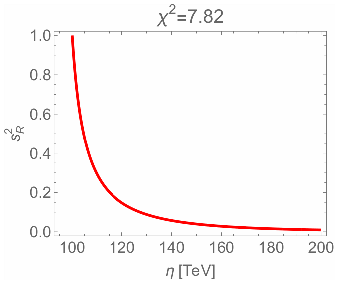
Figure 2.
Left panel: Energy-to-entropy ratio in eV, normalized by , as a function of . This quantity freezes at temperature . Right panel: Plot of for TeV.
Figure 2.
Left panel: Energy-to-entropy ratio in eV, normalized by , as a function of . This quantity freezes at temperature . Right panel: Plot of for TeV.
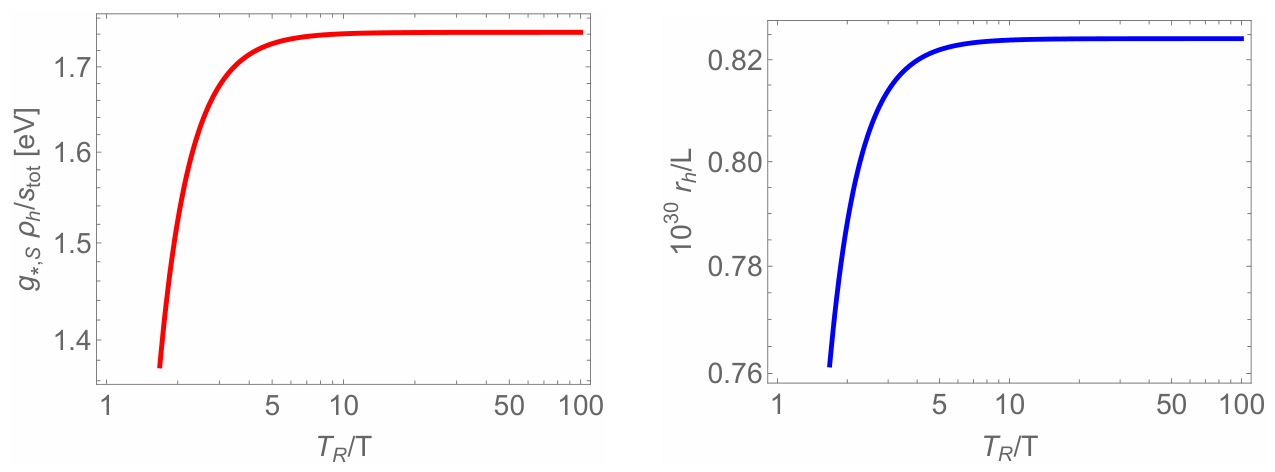
Figure 3.
Contour lines of in the plane for and . At the pole: and .
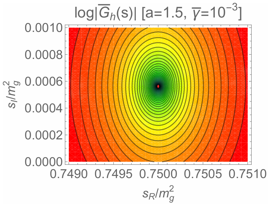
Figure 4.
Contour lines of the lifetime . The line for s corresponds to the present age of the universe, and s to the lower bound from cosmological observations.
Figure 4.
Contour lines of the lifetime . The line for s corresponds to the present age of the universe, and s to the lower bound from cosmological observations.
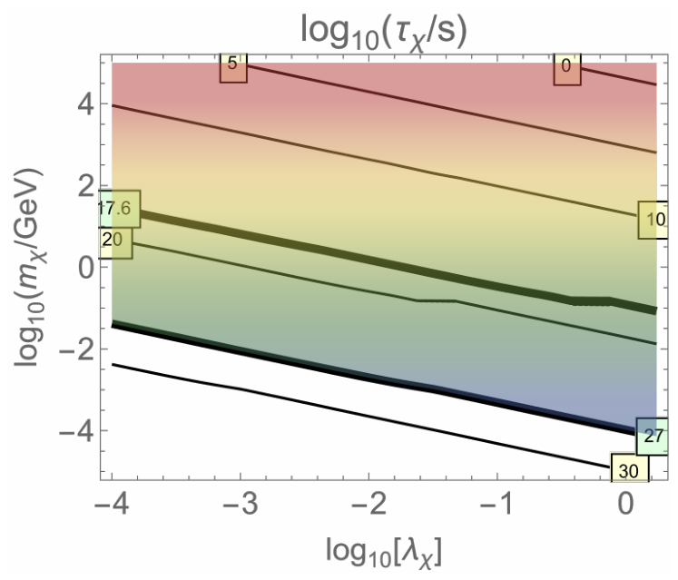
Figure 5.
The white region in the plane is allowed, as there and s.
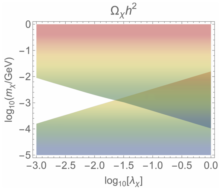

Table 1.
Summary of the boundary conditions for the gauge fields in the custodial model.
| Massless | , | |
| Massive | , | — |
Table 2.
Summary of the range of values of the fundamental parameters of the theory.
| Fundamental parameters | |
|---|---|
| DM mass | |
| 5D Planck mass | |
| Inflaton mass | |
Disclaimer/Publisher’s Note: The statements, opinions and data contained in all publications are solely those of the individual author(s) and contributor(s) and not of MDPI and/or the editor(s). MDPI and/or the editor(s) disclaim responsibility for any injury to people or property resulting from any ideas, methods, instructions or products referred to in the content. |
© 2026 by the authors. Licensee MDPI, Basel, Switzerland. This article is an open access article distributed under the terms and conditions of the Creative Commons Attribution (CC BY) license (http://creativecommons.org/licenses/by/4.0/).
Copyright: This open access article is published under a Creative Commons CC BY 4.0 license, which permit the free download, distribution, and reuse, provided that the author and preprint are cited in any reuse.