Direct Quantum Inversion: Reconstructing Underlying Dynamics from Kinematical Ensemble Measurements

1. Introduction

Could Isaac Newton have formulated the theory of gravity without access to Kepler’s laws of planetary motion? Although we may not know for certain, we know for sure that Newton needed to rely on empirical findings that described motion within a gravitational field. Kepler summarized the planetary motion (kinematics, or description of the motion), which Newton utilized to formulate the gravitational force (dynamics, or the cause of change in motion).

Parallel to this in the quantum domain, Planck [1], Rydberg [2], Ritz [3], and others helped outline the atomic transition laws experimentally. Based on such laws, and still within the realm of kinematics, Bohr [4] and Sommerfeld [5] charted the old quantum theory in terms of angular momentum quantization, conforming with de Broglie’s matter wave idea [6]. The field of quantum dynamics then opened a new era: first and foremost, through the work of Heisenberg in 1925 (matrix mechanics) [7] as motivated by empirical relations in atomic spectra—soon to be followed by Schrödinger’s dynamics (wave mechanics) [8], via his renowned equation, as motivated by de Broglie’s matter wave [6] and Einstein’s quantized radiation energy [9].

Because the quantum dynamical equation evolves the wavefunction, the dynamics dictate the kinematics (characterization of the state itself). But the inverse is also of great value. As a trivial example in classical mechanics, if a point mass is observed moving in space, its motion can be summarized by recording its position vectors, ${\mathit{x}}_i$ at discrete time intervals, $t_i$. If this temporal data is sufficiently dense, it can lead to an accurate equation of the orbit by modeling it with a parametric function $\mathit{x}(t;\overrightarrow{\theta })$ to estimate the optimal value of free parameter vector $\overrightarrow{\theta }$ and the uncertainty associated with it. Subsequently, vectors of velocity $\dot{\mathit{x}}(t)$, acceleration $\ddot{\mathit{x}}(t)$, and so forth can be derived. This complete description of the state of the motion (kinematics) can lead to determination of the force vector (dynamics) when Newton’s definition of force, $\mathit{F}=m\ddot{\mathit{x}}$, is combined. Alternatively, the system’s state of motion at an arbitrary time can be described by providing positions and momenta of its constituents (the phase space).

When Kepler analyzed his records of planetary positions over time, he realized he could fit the points on the orbit by a function, $\mathit{x}(t;\overrightarrow{\theta })$, which proved to be the equation of ellipses with parameters being eccentricity and semimajor axis. This purely kinematical description of physical trajectories helped Newton to formulate the force of gravity, in accordance with his definition of force.

The utility of such a direct kinematical approach appears to be missing from the current undertakings in the field of quantum theory—which is the main subject of this work as a novel line of inquiry. Such endeavors are envisaged to begin by observing and measuring a collection of many identically prepared quantum state samples, forming a pure ensemble. In this work, whenever a reference to an “ensemble” is made, a “pure ensemble” is intended, with all its members sharing a single common wavefunction, $\Psi (\mathit{x},t)$.

2. Utility of the Wavefunction

A core postulate of quantum mechanics dictates that the totality of a system's physical state is encoded within its wavefunction. Extracting much of this information is mathematically straightforward: for instance, projecting the wavefunction onto the eigenfunctions of an observable yields the probability amplitudes for that observable's spectrum. This is a direct consequence of the self-adjoint nature of quantum observables, which guarantees a complete, mutually orthogonal set of eigenfunctions. Because the functional forms of these eigenstates—such as those for linear momentum, angular momentum, and spin—are uniquely known independent of the specific system, their corresponding probability distributions are immediately accessible once the wavefunction is known.

The above reminder of simple quantum facts emphasizes that within our kinematical framework, directly reconstructing the unknown wavefunction or the density function from empirical data, followed by determination of the potential function, is imperative. Because the Hamiltonian operator is tied to the system's specific, unknown potential, its eigenfunctions cannot be determined a priori, and the system's dynamics remain hidden.

A detailed exploration of the reconstruction of such underlying dynamics is explained ahead.

3. Quantum Kinematic Practices

Because all accessible information about a system is encoded in its wavefunction, this state vector provides the natural foundation for characterizing the system's underlying dynamics. Since the wavefunction is directly related to the density in stationary states, empirically mapping the purely kinematical features of the spatial probability density, $\rho \left(x\right)$, across a well-prepared ensemble allows the wavefunction—and hence the underlying potential—to be reconstructed. Operationally, this framework begins with an analysis of ground-state position data to identify one or more candidate density functions that fit the data with reasonable statistical goodness-of-fit metrics. We then demonstrate that incorporating empirical excited-state energy eigenvalues, $E_n$, and comparing them against their theoretical predictions, provides a substantial gain in discriminating power—sufficient to break the deadlock and isolate the true density, and thus the true underlying potential.

3.1. The Position Data

As an example, consider the quantum state of a point mass, characterized through observation of a pure ensemble of $\mathcal{N}$ samples, all prepared in the same stationary state, with wavefunctions given by:

$${{\psi }_n(x,t)= \psi }_n(x) { e}^{-{\displaystyle \frac{i}{\hslash }}{E}_{n}t}$$

(1)

where ${\psi }_n(x)$ is the $n$^th eigenfunction of the Hamiltonian operator, with energy eigenvalue $E_n$, satisfying:

$$H{\psi }_n(x)=E_n{\psi }_n(x)$$

(2)

and the time-independent Hamiltonian (in 3D notation) given by:

$$\widehat{H}={\displaystyle \frac{-{\hslash }^2}{2m}}{\nabla }^2+V\left(\widehat{\mathit{x}}\right).$$

(3)

Measuring the particle position across the ensemble—simultaneously or one sample at a time—yields $\mathcal{N}$ coordinates $x_i$, where $i$ is the sample index. For simplicity, we restrict the discussion to a one-dimensional spatial formulation, which is extended to three dimensions in the third example later.

These position coordinates can be summarized as a histogram with bin width $\mathsf{\Delta }x$. Since all samples share the same stationary state, the resulting profile carries no time dependence and is expected to mirror the continuous function ${|\psi }_n(x){|}^2$—the probability density of finding the particle within the interval $\left[x,x+\mathsf{\Delta }x\right]$. To empirically determine this functional form, the data distribution can be fitted using a parametrized trial density function, ${\rho }_n\left(x;\overrightarrow{\theta }\right)$, with $\overrightarrow{\theta }$ the vector of fit parameters.

Although hybrid states are neither needed nor discussed in this work, a superposition of the time-dependent stationary states in Equation (1) constitutes the most general wavefunction for a quantum system:

$$\Psi (x,t)=\sum _n{C}_n{\psi }_n(x,t)=\sum _n{C}_n{\psi }_n(x) e^{-{\displaystyle \frac{i}{\hslash }}{E}_{n}t}$$

(4)

which satisfies the Schrodinger equation:

$$\widehat{H} \Psi \left(x, t\right)=i\hslash {\displaystyle \frac{\partial }{\partial t}}\Psi \left(x, t\right).$$

(5)

3.2. Fitting Techniques

Standard fitting procedures, such as binned ${\chi }^2$ minimization techniques, are functionally appropriate for this task. However, more advanced approaches, such as the un-binned Negative Log-Likelihood (NLL) method [10,11], are available to bypass the structural resolution losses of binning by processing all discrete data points directly. Crucially, the NLL framework inherently accommodates normalization, physical boundary conditions, and global constraints within a single unified formulation, the mathematical architecture of which is reviewed in Appendix A.

While the ${\chi }^2$ method is generally less effective for sparse datasets—as it reduces continuous positional information to static bin-centered counts—the operational advantages of both approaches are compared directly through the synthetic validations presented in the examples ahead. For highly complex or uncharacterized distributions where standard parametric ansatzes may prove inadequate, an alternative fallback methodology is reviewed in Appendix B. This approach utilizes an ansatz-free, non-parametric fitting technique based on Kernel Density Estimation (KDE) [12,13]. This non-parametric alternative retains the full physical utility that an analytical functional form would provide; although it relinquishes an explicit closed-form algebraic expression, all density information remains fully preserved and accessible via continuous numerical arrays and callable computational routines.

3.3. System and Notations

Although all stationary states can be studies by the methods of this work, preparing the system in its ground state is the most desirable configuration for this investigation, as it is the most empirically accessible state and typically possesses the least complicated wavefunction. Consequently, the functional form of the corresponding probability density function, ${\rho }_0\left(x;\overrightarrow{\theta }\right)$, is structurally simplified and less challenging to optimize against empirical data. From here on, we refer to such density function by $\rho \left(x;\overrightarrow{\theta }\right)$ for brevity, dropping the “0” subscript.

Assuming the underlying potential function lacks explicit time dependence, the parameters can be defined via the vector $\overrightarrow{\theta }=\left\{{\theta }_1,{\theta }_2,{\theta }_3,\dots \right\}$, which denotes the complete set of free parameters of the trial density function to be optimized through statistical data fitting.

It is crucial to emphasize that, throughout this work, expressions such as "measuring" or "determining" a parameter value denote estimating its optimal value through a statistical fit to the empirical data. This optimization process simultaneously yields both the parameter estimate and its associated statistical variance. Exceptional cases exist, however, where strict analytical determination replaces statistical estimation, rendering the resulting values exact and error-free. Such instances arise directly from rigid boundary conditions or fundamental physical laws. An example of the former occurs when a particle is confined to an infinite potential well, which dictates that its probability density function must vanish identically at the boundaries. An example of the latter arises when a trial-function parameter can be evaluated analytically by exploiting the variational principle—specifically, the stationary property of the ground-state energy—by setting its corresponding derivative to zero. Barring such exact geometric or physical cases, the extraction of a parameter via empirical data fitting invariably entails an optimization process that couples an optimal value with a quantifiable statistical uncertainty. Similarly, other modalities of empirical characterization, such as direct energy measurements, are truly only estimations rather than determinations, owing to unavoidable empirical uncertainties—although "determination" terminology remains commonly used.

3.4. Wavefunction-Density Relation

Our choice of ground state, being a stationary state, has the further advantage that once its density function is measured, the wavefunction form will follow. While the formulation remains identical for any excited stationary state, this work focuses exclusively on the ground state unless explicitly stated otherwise.

Since the system is in its ground state described by its stationary wavefunction given by Equation (1), our density function, $\rho \left(x;\overrightarrow{\theta }\right)$, is related to the spatial component of the wavefunction ${\psi }_0(\mathit{x})$ by $\rho \left(x;\overrightarrow{\theta }\right)={|\psi }_0(x){|}^2$, or:

$${\psi }_0(x)=\sqrt{\rho \left(x;\overrightarrow{\theta }\right)}.$$

(6)

Equation (6) follows only if ${\psi }_0(x)$ is real , which is valid due to its being an eigenfunction of the Hamiltonian in Equation (2) where $H$ and $E_n$ are real entities, and $n=0$ corresponds to the ground state.

Since the unique energy of the stationary ground state, $E_0$, can be readily measured, the physical characterization of the wavefunction is complete, as we can represent, using Equation (1), the full time-dependent stationary state as:

$${\psi }_0(x,t)=\sqrt{\rho \left(x;\overrightarrow{\theta }\right)}{ e}^{-{\displaystyle \frac{i}{\hslash }}{E}_{0}t}.$$

(7)

From this, extracting any information about the system is available—given that the density determination from fit to the position data distribution is completed.

4. Dynamics from Kinematics (Quantum Kinematics or Inversion)

Leveraging the stationary property of the ground-state energy expectation value, we can formulate the quantum inversion procedure as follows. This stationary property [14,15] is further employed in one of our examples as a consistency check.

4.1. Potential as a Function of Position

At this stage, we assume the ground-state energy $E_0$ has been measured, and that the parameter vector $\overrightarrow{\theta }$ optimizing the density function ${\rho }_0\left(x;\overrightarrow{\theta }\right)$ in its fit to the data has been determined. In general, the energy expectation value $⟨E⟩$ is defined by:

$$⟨E⟩\equiv {\displaystyle \frac{\int dx {\Psi }^{*}(x,t) \widehat{H} \Psi (x,t)}{\int dx {\Psi }^{*}(x,t)\Psi (x,t)}} .$$

(8)

Using this relation together with the wavefunction of Equation (6) and the Hamiltonian of Equation (3), and noting that the energy expectation value must equal the unique ground-state energy $E_0$ for our stationary state, we obtain:

$$⟨E_0⟩\equiv {\displaystyle \frac{\int dx \left[\frac{-{\mathrm{\hslash }}^2}{2m}\sqrt{\rho \left(x;\overrightarrow{\theta }\right)} {\nabla }^2\sqrt{\rho \left(x;\overrightarrow{\theta }\right)}\right]+\int dxV\left(x\right) \rho \left(x;\overrightarrow{\theta }\right)}{\int dx \rho \left(x,\overrightarrow{\theta }\right)}}=E_0.$$

(9)

This yields a relation among three integrals, which in turn implies a corresponding relation among their integrands. Solving this relation for the potential function, we obtain:

$$V\left(\mathit{x}\right)={\displaystyle \frac{{\mathrm{\hslash }}^2}{2m}}{\displaystyle \frac{{\nabla }^2\sqrt{\rho \left(x;\overrightarrow{\theta }\right)}}{\sqrt{\rho \left(x;\overrightarrow{\theta }\right)}}}+E_0.$$

(10)

A few straightforward algebraic steps on Equation (10) give an alternative expression for the potential:

$$V\left(\mathit{x}\right)={\displaystyle \frac{{\mathrm{\hslash }}^2}{2m}}\left({{\displaystyle \frac{1}{2}}\nabla }^2\mathrm{l}\mathrm{n}\rho \left(x;\overrightarrow{\theta }\right)+{\displaystyle \frac{1}{4}}{\left.\left|\mathsf{\nabla } \mathrm{l}\mathrm{n}\rho \left(x;\overrightarrow{\theta }\right)\right.\right|}^2\right)+E_0.$$

(11)

These position-dependent expressions for the potential energy—representing the underlying dynamics of the system—are now fully determined once the data-optimized density functions are provided.

4.2. Potential for Internal Degrees of Freedom

While the derivation leading to Equations (10) and (11) formulates the potential in terms of the empirical density function, that analysis restricts the dynamics to dependence on spatial coordinates alone. Quantum mechanics, however, features internal degrees of freedom—such as spin—in multilevel systems, whose dynamics extend beyond spatial coordinates. Additionally, multilevel systems can involve multiple energy channels, for which the relation $⟨E_0⟩=E_0$ is not quite meaningful, and Equation (9) may therefore be inappropriate. An alternative scheme is thus required to accommodate internal degrees of freedom.

For this purpose, in 3D notation, we define the function $W(\mathit{x},t)$ by:

$$W\left(\mathit{x},t\right)=\left({\displaystyle \frac{{\mathrm{\hslash }}^2}{2m}}{\nabla }^2+i\mathrm{\hslash }{\displaystyle \frac{\partial }{\partial t}}\right)\Psi \left(\mathit{x},t\right).$$

(12)

Comparing this with the Schrödinger Equation (5) and the Hamiltonian (3), and rearranging, yields:

$$V\left(x\right)={\displaystyle \frac{W\left(x,t\right)}{\Psi \left(x,t\right)}}.$$

(13)

This alternative formulation of the potential recovers the previous result of Equation (10) when Equation (7) is substituted into Equations (10) and (11). However, by explicitly retaining the time derivative, Equation (13) possesses the generality needed to accommodate internal degrees of freedom. Although the spatial coordinates of the system have no bearing on the dynamics of internal degrees of freedom, time evolution remains unavoidable—as will be seen in one of the examples ahead.

4.3. General Analysis Methods

The operational execution of this inversion framework can be formalized into the following procedural steps, though occasional variations may become necessary:

• Ansatz Formulation: Propose several trial density functions, ${\rho }_i\left(x;\overrightarrow{\theta }\right)$, consistent with the geometric shape, symmetries, and boundary conditions observed in the empirical ground-state position histogram.
• Parametric Optimization: Where free parameters are involved, fit each trial density to the empirical position-data distribution to estimate the optimal structural parameter vector, $\overrightarrow{\theta }$.
• Statistical Evaluation: Tabulate goodness-of-fit metrics for each candidate using both binned ${\chi }^2$ and un-binned Negative Log-Likelihood (NLL) methods. Retain all candidates with even marginally acceptable fit statistics for downstream validation, even if a single model appears statistically preferred.
• Potential Function Reconstruction: Substitute each optimized trial density into Equation (10), (11), or (13), as appropriate, to compute its uniquely reconstructed potential function.
• Spectral Prediction: Use these potentials to construct the corresponding Hamiltonians and solve the eigenvalue problem of Equation (2) to obtain the theoretical energy spectrum for each candidate. (Numerical grids should be employed where closed-form analytical solutions are unavailable.)
• Breaking Statistical Deadlocks (Informal): The system can also be studied via its excited states, allowing an empirical measurement of the energy spectrum, $E_n$. Notably, the detailed wavefunctions of the excited states need not be determined for this purpose. For a charged particle, such a measurement can be carried out spectroscopically: exposing the ensemble to broadband continuous electromagnetic radiation and identifying the resulting dark absorption lines in the transmitted spectrum yields the empirical energy eigenvalues directly.

These measured values can then be compared against the theoretical spectrum predicted by each candidate density in turn. Ultimately, a density candidate is acceptable only if the potential it implies satisfies two independent criteria: an acceptable statistical goodness-of-fit to the position data, and a predicted energy spectrum consistent with the empirically observed eigenvalues. Agreement on both fronts provides a substantially more stringent test than either criterion alone, offering a natural route to breaking a deadlock left unresolved by position data alone.

7.

Breaking Statistical Deadlocks (Formal): A complete treatment of formal statistical methods for this purpose is beyond the scope of this paper, as each dataset presents its own complexities. For rigorous treatment of complex, real-world datasets, we refer the reader to standard references such as [16,17]. The trial function may involve no free parameters or several; the latter case requires additional care, since parameter correlations and subjective Bayesian methods—involving priors, likelihood functions, and their mutual correlations—can enter as part of a multidimensional statistical analysis.

Furthermore, the dual nature of the decision—combining position-distribution modeling with spectral information—requires careful statistical treatment. When spectral lines are well separated, the quantized nature of the spectral sub-data can resolve a deadlock straightforwardly; when lines lie close together, however, a more elaborate statistical analysis is needed.

The Bayesian concept of priors offers a natural iterative refinement scheme: one subset of the data is analyzed to obtain a posterior likelihood, which is then adopted as an updated prior and combined with a further, previously unused, subset of the data to obtain a new posterior. Given a sufficiently large dataset, this iterative sharpening can in principle be continued without limit, allowing the analysis to converge to an arbitrarily confident decision.

A further complication is that the excited-state energies enter as quantized (discrete) values, which is atypical for standard Bayesian treatments built around continuous likelihoods. In our case, the combined likelihood is therefore a product of two functions of distinct character—one continuous (from the position data) and one discrete (from the energy spectrum)—a hybrid structure that should be handled explicitly rather than assumed away.

The spectral aspect of our framework parallels laboratory and astronomical spectroscopy, where researchers analyze atomic and molecular spectral profiles for identification. Because atomic structure is governed by the well-known Coulomb potential, the corresponding theoretical spectra can be deduced analytically for simple elements and computed numerically for complex atoms and molecules. Additionally, the spectral patterns of known elements and some molecules have already been recorded through prior laboratory measurement, so observers need only compare these established baselines against new empirical measurements to identify constituent elements.

A key distinction in our framework, however, is that we begin with a pool of multiple candidate potential functions satisfying the initial statistical fitting stage, rather than a single established law. Furthermore, because no prior baseline data exists for the uncharacterized system under study, this comparative sequence must be systematically repeated for each viable candidate.

4.4. Significance of Excited-state Energies

Relying solely on the ground-state energy is insufficient as a discriminator for closely competing density candidates, given that distinct physical systems can exhibit identical ground-state eigenvalues despite having vastly different excited-state ladders. A prime example of this ambiguity occurs naturally within Supersymmetric Quantum Mechanics (SUSY QM) [18,19]. Here, the conventional harmonic potential $V_1\left(x\right)={\displaystyle \frac{1}{2}}{x}^2$ (under the parameter constraints ($\hslash =m=\omega =1$) is paired with a deformed, non-harmonic partner potential, $V_2\left(x\right)$, expressed as:

$$V_2\left(x\right)={\displaystyle \frac{1}{2}}{x}^2+{\displaystyle \frac{2}{\sqrt{\pi }}}{\displaystyle \frac{x{e}^{-x^2}}{\gamma +\frac{\sqrt{\pi }}{2}\mathrm{erf}\left(x\right)}}+{\displaystyle \frac{e^{-2x^2}}{{\left(\gamma +\frac{\sqrt{\pi }}{2}\mathrm{erf}\left(x\right)\right)}^2}} .$$

Despite sharing a common ground-state energy of $E_0={\displaystyle \frac{1}{2}}$ , the two systems exhibit entirely different excited-state spectra. Although these two specific partner potentials possess drastically different analytical formulations—making them unlikely to emerge simultaneously within the same parametric candidate pool—it is highly probable that closely formulated potential variants will exhibit nearly identical ground-state energies within experimental error bars while remaining highly distinguishable in their excited states. Consequently, incorporating excited-state energies is a practically important component of our inversion framework, providing the necessary spectral resolution to break statistical deadlocks and differentiate the true governing potential from competing parametric density candidates.

4.5. Numerical Schemes

When data scarcity in sample size $\mathcal{N}$, suboptimal position resolution ${\sigma }_i$, or intricate quantum interactions make isolating a single candidate statistically unreliable, alternative pathways still allow for successful reconstruction. In fact, the underlying potential can be effectively modeled even when mapping a closed-form functional representation of the density proves unfeasible. In this numerical form, the recovered density functions are exactly like an analytical expression for practical applications. This is achieved through advanced non-parametric fitting methods that bypasses the need for a global structural ansatz. By employing spatial field methods, these techniques trade global equations for localized numerical grids and callable functions [12,13]. Some of the details of this model-free methodology are reviewed in Appendix B.

Crucially, once the potential is known, the Hamiltonian (3) is completely defined, leaving the dynamics of the system fully resolved.

5. Examples

The following sections demonstrate general kinematical inversion methods across several case studies. Specifically, Examples 1 and 5 utilize synthetic datasets with known underlying dynamics to benchmark the framework, providing a baseline before addressing the distinct challenges of experimental data. These synthetic analyses rely on fitting a trial density function $\rho \left(x;\overrightarrow{\theta }\right)$ using two distinct optimization approaches: the binned ${\chi }^2$ method [20] and the un-binned Negative Log-Likelihood (NLL) technique [10,11]. Unlike the histogram-based ${\chi }^2$ criterion, the NLL approach proceeds without binning by minimizing the negative logarithm of the joint likelihood function to resolve the free parameter vector, $\overrightarrow{\theta }$, by determining theirs optimal values. The mathematical architecture, core parameters, and multi-metric evaluation criteria of this un-binned optimization framework are reviewed in Appendix A. Crucially, the NLL formulation inherently accommodates normalization scaling, physical boundary conditions, and global constraints within a single objective function, while the non-parametric fallback options necessary for handling complex or arbitrary empirical distributions are outlined in Appendix B.

5.1. Example 1 (Particle-in-a-Box)

5.1.1. Synthetic Data and Candidate Density Functions

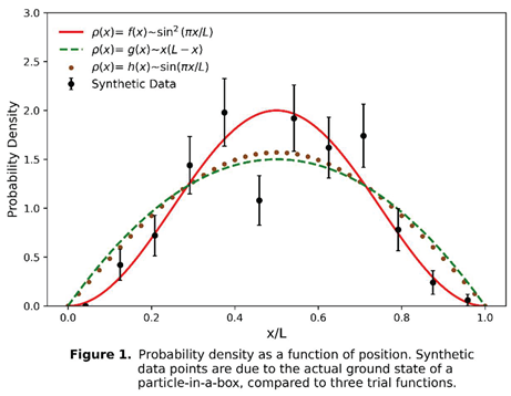
In this first example, we consider a particle confined to a one-dimensional box of length $L$, in its ground state. To exercise our method for determining the functional form of the potential inside the box, we use synthetic data. The binned spatial distribution of the position data, $x_i$, is displayed as points with error bars in Figure 1—the result of simulated position measurements generated assuming the true ground-state density function of a particle in a box (infinite potential well), with vanishing potential inside the box. If parametrized trial density functions were proposed, their optimal parameter values would be found by fitting them to the data using the minimum-${\chi }^2$ and un-binned NLL methods described previously. In this specific case, however, we propose trial functions that are unparametrized; we therefore simply compare the structural geometry of each candidate function directly against the synthetic data distribution, as shown in Figure 1.

For this evaluation, the complete absence of free parameters is not problematic, since the trial functions selected below are already analytically constrained to satisfy the strict boundary conditions at the two ends of the box. We therefore need only determine the statistical goodness-of-fit of each candidate density function to the data distribution. The first trial function is defined as:

$$\rho (x)=f(x)=N{\mathit{sin}}^2{\displaystyle \frac{\pi }{L}}x$$

(14)

which is expected to provide the optimal fit to the data, since it matches the true underlying particle-in-a-box density function. This baseline is compared against two alternative geometric test functions:

$$g(x)=Nx(L-x)$$

(15)

and:

$$h\left(x\right)=N\sin \left({\displaystyle \frac{\pi x}{L}}\right).$$

(16)

The hard box boundary conditions are satisfied identically by all three trial expressions.

5.1.2. Fitting Density Function Candidates to the Data

Visual inspection of Figure 1 indicates that the trial density function $f\left(x\right)$ follows the data more closely than the alternative options $h\left(x\right)$ and $g\left(x\right)$. However, this qualitative observation requires quantitative confirmation via goodness-of-fit metrics evaluated against the empirical data distribution. The summary of the results of these comparisons is recorded in Table 1 below, which reports the statistical metrics from both the binned ${\chi }^2$ method and the un-binned Negative Log-Likelihood (NLL) framework [10,11]. A measurement uncertainty ${\sigma }_i$ is assigned to each position datum $x_i$, to account for experimental effects.

The following notes about the parameters recorded in Table 1 may be instructive: (See Appendix A for more detailed information.)

○

The Negative Log-Likelihood is defined as $\mathrm{NLL}=-\sum \ln \mathrm{pdf}\left(x_i\right)$, where a lower (more negative) value indicates a more optimal fit.

○

The information criteria are expressed as $\mathrm{AIC}=2k-2\ln L$ and $\mathit{BIC}=k\cdot \ln \left(N\right)-2\ln L$, where $k$ denotes the number of free parameters. Because $k=0$ for these fixed baselines, the AIC and BIC values are identical and track $-2\ln L$ directly.

○

The Kolmogorov–Smirnov (KS) test evaluates the goodness-of-fit by comparing the empirical cumulative distribution function (CDF) of our $\mathcal{N}=200$ samples against each model's closed-form CDF. $\mathrm{K}\mathrm{S}$ test compares the empirical CDF of our 200 samples to each model's closed-form CDF. $f\left(x\right)$ has by far the best (highest) $p$-value—as expected, since its form is the same as the true generating distribution. $g\left(x\right)$ is rejected at the 5% level ($p=0.028$); $h\left(x\right)$ is borderline ($p=0.062$).

○

The likelihood ratio metric $\mathsf{\Delta }\left(-2\ln L\right)$ is calculated relative to the optimal model, $f\left(x\right)$, via $2\left({\mathrm{NLL}}_i-{\mathrm{NLL}}_{\mathrm{best}}\right)$, which quantifies the statistical divergence of model $i$ from the true generating distribution.

○

Reading across all five statistical metrics, the results are completely coherent. The $f\left(x\right)$ trial function is clearly favored; its structure is identical to the true generating distribution, yielding the highest p-value (${\chi }^2/\mathrm{DOF}\approx 0.5$, comfortably consistent; $p\left({\chi }^2\right)$ and $p\left(\mathrm{KS}\right)$ are both large). Conversely, $g\left(x\right)$ is definitively rejected at the 5% significance level ( ${\chi }^2/\mathrm{DOF}\approx 2$, with both p-values dropping below $0.05$). The $h\left(x\right)$ candidate represents an intermediate case, appearing borderline but statistically consistent via the binned ${\chi }^2$ test ($p=0.106$) while sitting right at the critical edge of rejection under the bin-free $\mathrm{KS}$ test ($p=0.067$).

○

The fact that a binned test (${\chi }^2$), a bin-free test ($\mathrm{KS}$), and a likelihood-based comparison (NLL/AIC) all converge on a single ranking makes the selection of $f\left(x\right)$ highly robust.

All metrics recorded in Table 1 support the conclusion that $f\left(x\right)$ represents the optimal model, $g\left(x\right)$ the worst, and $h\left(x\right)$ an intermediate option. A subsequent power analysis indicates that, if higher statistical power is required to confidently reject these untrue trial functions, the empirical dataset size must be expanded. Letting $\mathcal{N}$ denote the total number of position-coordinate data points randomly generated from the true distribution, the binned ${\chi }^2$ power test evaluating the sample size required to exclude the more resilient candidate, $h\left(x\right)$, is summarized in Table 2 below:

In Table 2, the power of rejection is defined as the fraction of trials in which $h\left(x\right)$ is correctly rejected by the criterion on the p-value ($p<0.05$). At our current sample size of $\mathcal{N}=200$, the framework correctly distinguishes $f\left(x\right)$ from $h\left(x\right)$ approximately 72% of the time; conversely, roughly one in four experiments would fail to reject $h\left(x\right)$ even though $f\left(x\right)$ is the true underlying generator. This statistical behavior aligns closely with the results shown in Table 1, where $p=0.106$ for $h\left(x\right)$ corresponds to a miss rate of 28%. We can further project the empirical data requirements needed to achieve 80% and 95% rejection power. Based on the power analysis results recorded in Table 2, these milestones require sample sizes of approximately $\mathcal{N}\approx 220–230$ and $\mathcal{N}\approx 320–350$, respectively.

5.1.3. Potential Functions

Following the general analysis steps outlined in Section 4.3, the framework extracts the potential function corresponding to each candidate density function. For the statistically favored option, $f(x)$, given by Equation (14), calculating the potential function via Equation (10) yields:

$$V_f(x)={\displaystyle \frac{{\mathrm{\hslash }}^2}{2m}}{\displaystyle \frac{\frac{{\partial }^2}{\partial x^2}\mathrm{s}\mathrm{i}\mathrm{n}\frac{\pi }{L}x}{\mathrm{s}\mathrm{i}\mathrm{n}\frac{\pi }{L}x}}+E_0=-{\displaystyle \frac{{\mathrm{\hslash }}^2{\pi }^2}{2m{L}^2}}+E_0 \hspace{1em}⟶\hspace{1em}0.$$

(17)

Applying the same procedure via Equation (10) to the remaining two trial functions yields the corresponding potentials for the $g(x)$ and $h(x)$ density functions:

$$V_g(x)={\displaystyle \frac{-{\hslash }^2}{mx\left(L-x\right)}}+E_0 \hspace{1em}⟶\hspace{1em}{\displaystyle \frac{-{\hslash }^2}{mx\left(L-x\right)}}$$

(18)

and:

$$V_h(x)=-{\displaystyle \frac{1}{4}}\left({\displaystyle \frac{{\pi }^2{\hslash }^2}{2m{L}^2}}\right)\left(1+{\csc }^2{\displaystyle \frac{\pi }{L}}x\right)+E_0 \hspace{1em}⟶\hspace{1em}-{\displaystyle \frac{1}{4}}\left({\displaystyle \frac{{\pi }^2{\hslash }^2}{2m{L}^2}}\right){\csc }^2\left({\displaystyle \frac{\pi }{L}}x\right).$$

(19)

The rightward arrows in the Equations (17) – (19) denote the effective functional forms isolated after omitting dynamically inconsequential additive constant energies as the energy ladder spacing remains the same.

Equation (17) indicates a constant potential for density function $f\left(x\right)$. Notably, this constant potential vanishes under the condition ${E_0}^{(n=1)}={\displaystyle \frac{{\pi }^2{\hslash }^2}{{2mL}^2}}$, which matches exactly the standard ground-state energy from the particle-in-a-box spectrum $E_n={\displaystyle \frac{{n^2\pi }^2{\mathrm{\hslash }}^2}{{2mL}^2}}$. Consequently, the baseline potential can be taken as zero without loss of generality, since an additive constant merely shifts the zero-point energy—leaving the wavefunctions and underlying dynamics unaffected, as a constant always commutes with the Hamiltonian—unless the shift is large enough to convert a bound state into a scattering state, or vice versa. Provided the sign of $\left(V\left(x\right)-E\right)$ remains unchanged, any constant shift in the potential is dynamically inconsequential.

Based on the analysis steps in Section 4.3, we can use these potential functions to calculate the energy spectra for the three candidates. The derivation of the energy eigenvalues for $V_g\left(x\right)$ is not as straightforward as for the constant $V_f\left(x\right)$. The full derivation is therefore presented in Appendix C, where $V_g\left(x\right)$ is shown to lead to a Heun-type ODE [21] that requires numerical calculation to obtain the excited-state energy eigenvalues, recorded in Table 3.

The potential $V_h\left(x\right)$, by contrast, proves to be a well-established variant of the trigonometric Pöschl–Teller potential [22] with exact, known solutions. Equation (19) represents a specific case of this trigonometric potential; crucially, it generates the exact ground-state density profile of Equation (16) if and only if its structural coupling coefficient matches the value appearing in Equation (19). This functional family plays a prominent role in Supersymmetric Quantum Mechanics (SUSY QM) [19], and features heavily in superstring theory. Its exact energy eigenvalues are likewise recorded in Table 3.

5.1.4. Finding the Best Candidate

In this example, three distinct trial density functions were evaluated. While the statistical metrics in Table 1 point to $f\left(x\right)$ as the optimal choice, this advantage is only statistically decisive in high-resolution regimes with large data samples ($N>200$, $\sigma \le 0.05$ for $x\in \left[\mathrm{0,1}\right]$)—as evidenced by the rejection-power values in Table 2. In less-than-ideal empirical environments, alternative models such as $h\left(x\right)$ can remain statistically viable competitors within acceptable goodness-of-fit metrics, making it challenging to isolate the true potential from ground-state position data alone.

Consistent with the general procedural framework established in Section 4.3, we showed that any such statistical deadlock can be broken by mapping each candidate density to its corresponding quantized excited-state energy spectrum. For this case study, the resulting excited-state energy ladders are recorded in Table 3. Comparing these theoretical spectra directly against the system's empirical spectroscopic measurements allows the true potential to be uniquely isolated. Exact analytical eigenvalue solutions were obtained for the $f\left(x\right)$ and $h\left(x\right)$ density candidates; for the $g\left(x\right)$candidate, however, numerical computation was required, as reviewed in Appendix C.

Similarly, when deriving the potential functions from the density candidates, the numerical grid routines outlined in Appendix B remain the primary computational pathway whenever an analytical potential function cannot be found—for instance, when resolving completely unknown or non-analytic quantum systems. For this example, however, that implementation was not required, as the potential functions were readily calculable analytically.

As recorded in the last column of Table 3, the quantized excited-state energies predicted by each trial density function yield distinct spectral values and spacings, enabling discrimination among the candidates. Comparing experimental excited-state measurements, $E_n$—once available—against these theoretical spectra can break any remaining statistical deadlock and isolate the true potential function. Energy-based information of this kind thus forms a powerful discriminator for uniquely determining the true underlying dynamics.

5.1.5. Checks for Consistency

The absence of free parameters in the three density functions above is understandable, since the boundary conditions at both walls were built directly into their functional forms. To check the internal consistency of the analysis framework, we artificially introduce a free parameter—a continuous exponent, $n$—into $f\left(x\right)$, forming the parametrized trial density function:

$$\rho (x;n)=N{\sin }^{2n}{\displaystyle \frac{\pi }{L}}x.$$

(20)

While $n=1$ recovers the baseline model derived previously, we now treat $n$ as a free variable in Equation (20) to test whether the framework correctly recovers this optimal value on its own. We calculate the energy expectation value and impose the stationarity condition. Consistent with the result of Equation (17), we set $V\left(x\right)=0$ and evaluate $⟨E_0⟩$ via Equation (9):

$$⟨E_0⟩={\displaystyle \frac{N\int dx\left[\frac{-{\mathrm{\hslash }}^2}{2m}\left({\sin }^n\frac{\pi }{L}x\frac{{\partial }^2}{\partial x^2}{\sin }^n\frac{\pi }{L}x\right)\right]}{N\int dx{\sin }^{2n}\frac{\pi }{L}x}}={\displaystyle \frac{{{\mathrm{\hslash }}^2\pi }^2}{{2mL}^2}}{\displaystyle \frac{n^2}{2n-1}}.$$

(21)

The stationarity condition applied to Equation (21), ${\displaystyle \frac{\partial ⟨E_0⟩}{\partial n}}=0$, admits two formal roots, $n=0$ and $n=1$; however, $n=0$ reduces $\rho \left(x;n\right)$ to a constant, violating the boundary conditions $\rho \left(0\right)=\rho \left(L\right)=0$. Thus $n=1$ emerges as the unique solution respecting the boundary conditions, consistent with the known ground-state density in Equation (14), for $V\left(x\right)=0$.

We now examine the implications of the alternative trial density function, $h\left(x\right)$, previously identified as a variant of the Pöschl–Teller potential with exact solutions, but shown in Section 5.1.1 to be a poor descriptor of the ground-state data. Selecting the functional form $\rho \left(x\right)\equiv h\left(x\right)=N\sin \left({\displaystyle \frac{\pi }{L}}x\right)$, as defined by Equation (16), yields poor visual and statistical fits to the empirical coordinate distribution, as seen in Figure 1 and Table 1.

This case—a candidate with poor statistical metrics, no adjustable shape parameters, and fixed boundary conditions—illustrates a broader requirement within the framework: an exceptionally poor-fitting candidate must, at this stage, either be refined by introducing free parameters or be discarded on statistical grounds alone. More importantly, though, examining $h\left(x\right)$'s exact mathematical properties alongside its poor statistical fit reveals a central conceptual point of quantum inversion: a candidate function can be a badly compromised fit to a given empirical dataset while remaining the exact, legitimate ground-state density of an entirely different physical system. It is precisely because the empirical data show no correspondence to that alternative potential's physical signature that $h\left(x\right)$ can be confidently ruled out here — its mathematical elegance as an exact solution to a different problem offers it no special exemption from the data.

5.2. Example 2 (Simple Harmonic Oscillator)

As a second example, consider a one-dimensional quantum system in which ensemble measurements of position, $x_i$, are used to construct the position probability distribution. We assume it is appropriate to model this empirical distribution with the following parametrized trial density function:

$$\rho \left(\mathit{x};\alpha \right)=N^2{e}^{- 2\alpha x^2}$$

(22)

where $\alpha$ is a free parameter, optimized by fitting this trial density to the empirical ensemble position-data distribution. Using Equation (11), the corresponding potential function for Equation (22) is found to be:

$$V\left(\mathit{x}\right)={\displaystyle \frac{{{2\mathrm{\hslash }}^2\alpha }^2}{m}}{x}^2-{\displaystyle \frac{{\mathrm{\hslash }}^2\alpha }{m}}+E_0.$$

(23)

This expression describes a quantum simple harmonic oscillator (SHO) potential plus an additive constant. This constant vanishes under the condition that $E_0$= ${\displaystyle \frac{{\mathrm{\hslash }}^2}{m}}\alpha$. If this relation is confirmed by the measured energy $E_0$ and the fitted parameter $\alpha$, the potential reduces to the standard SHO form:

$$V\left(\mathit{x}\right)={\displaystyle \frac{1}{2}}{m{\omega }^{2}x}^2$$

(24)

where, by comparison with Equation (23):

$$\omega ={\displaystyle \frac{2\mathrm{\hslash }\alpha }{m}}={\displaystyle \frac{2}{\mathrm{\hslash }}}{E}_0.$$

(25)

Any remaining constant shift is physically inconsequential as it merely realigns the zero-point energy, provided the sign of $\left(V\left(x\right)-E_0\right)$ remains unchanged. Finally, combining Equations (7) and (22), with the aid of Equation (25), the time-dependent ground-state wavefunction is:

$${\psi }_0(\mathit{x},t)=N{e}^{-{\displaystyle \frac{m\omega }{2\mathrm{\hslash }}}{x}^2-i{\displaystyle \frac{\omega }{2}}t}.$$

(26)

This aligns with the ground state of the conventional SHO model [14,15], as expected. Since this derived wavefunction satisfies the energy eigenvalue equation with eigenvalue $E_0={\displaystyle \frac{1}{2}}\mathrm{\hslash }\omega$, it corresponds precisely to the lowest energy state ($n=0$) of the standard spectrum, $E_n=(n+{\displaystyle \frac{1}{2}})\mathrm{\hslash }\omega$, resolving the exact analytical wavefunction.

Although the exact underlying potential has already been identified, we can demonstrate the self-consistency of the framework by imposing the stationarity condition to optimize the parameter $\alpha$ of the trial density function in Equation (22). From Equation (9), the energy functional evaluates to:

$$⟨E_0⟩={\displaystyle \frac{{\int }_{-\mathrm{\infty }}^{\mathrm{\infty }}dx\left[\frac{-{\mathrm{\hslash }}^2}{2m}\left(e^{-\alpha x^2}\frac{{\partial }^2}{\partial x^2}{e}^{-\alpha x^2}\right)+\frac{1}{2}{m{\omega }^{2}x}^2{e}^{-2\alpha x^2}\right]}{{\int }_{-\mathrm{\infty }}^{\mathrm{\infty }}dx{e}^{-2\alpha x^2}}}={\displaystyle \frac{{\mathrm{\hslash }}^2}{2m}}\alpha +{\displaystyle \frac{m{\omega }^2}{8\alpha }}.$$

(27)

Minimizing this expression according to ${\displaystyle \frac{\partial ⟨E_0⟩}{\partial \alpha }}=0$ yields $\alpha ={\displaystyle \frac{m\omega }{2\mathrm{\hslash }}}$, consistent with Equation (25) and recovering the same wavefunction as Equation (26). This independently confirms the exact physical solution through a variational check, assuming the potential of Equation (24).

5.3. Example 3 (Electronic States)

This third example shows one way in which the formalism can be applied to higher dimensions. Consider an electronic state described in spherical coordinates. Assume that ensemble measurements of the three-dimensional electron position, $x_i$, yield three separate marginal distributions in $r$, $\theta$, and $\phi$. To model these distributions, we introduce three independent trial density functions: $\rho \left(r;b\right)$, $\rho \left(\theta \right)$, and $\rho \left(\phi ;\alpha \right)$. The profiles of the empirical datasets suggest the following trial forms:

$$\begin{gathered} {\rho (r;b)=N_{r}r}^2{e}^{-br} \\ \rho (\theta )=N_{\theta }{\mathrm{s}\mathrm{i}\mathrm{n}}^2\theta \\ \rho (\phi ;\alpha )=N_{\phi }{\mathrm{c}\mathrm{o}\mathrm{s}}^2\left(\phi -\alpha \right) \end{gathered}$$

(28)

where the angular function $\rho \left(\theta \right)$ contains no free parameters. We assume fitting these functions to the three empirical distributions yields satisfactory results, achieving acceptable ${\chi }^2/\mathrm{DOF}$ at the optimized parameter values $b$ and $\alpha$. Consequently, the combined three-dimensional density function can be expressed as the product of these individual components:

$${\rho (r,\theta ,\phi ;b,\alpha )=N^{2}r}^2{e}^{-br}{\mathrm{s}\mathrm{i}\mathrm{n}}^2\theta {\mathrm{c}\mathrm{o}\mathrm{s}}^2 \left(\phi -\alpha \right)$$

(29)

where $N^2\equiv N_r{N}_{\theta }{N}_{\phi }$. Substituting this joint density function of Equation (29) into Equation (10) gives the three-dimensional potential function:

$$V\left(r\right)={\displaystyle \frac{{\mathrm{\hslash }}^2}{2m}}\left\{{\displaystyle \frac{{\nabla }^2\left[r{e}^{-\frac{b}{2}r}\mathrm{s}\mathrm{i}\mathrm{n}\theta \mathrm{c}\mathrm{o}\mathrm{s}\left(\phi -\alpha \right)\right]}{r{e}^{-\frac{b}{2}r}\mathrm{s}\mathrm{i}\mathrm{n}\theta \mathrm{c}\mathrm{o}\mathrm{s}\left(\phi -\alpha \right)}}\right\}+E_2={\displaystyle \frac{{-\mathrm{\hslash }}^{2}b}{m}}{\displaystyle \frac{1}{r}}+{\displaystyle \frac{{\mathrm{\hslash }}^2{b}^2}{8m}}+E_2.$$

(30)

As will be seen, $E_2$ denotes the energy of the first excited state ($n=2$) of hydrogen. As before, isolating the coordinate-dependent portion of the potential—by absorbing the remaining constant terms into a global shift of the energy scale—yields a pure Coulomb potential:

$$V\left(r\right)=-{\displaystyle \frac{{\mathrm{\hslash }}^{2}b}{m}}{\displaystyle \frac{1}{r}}.$$

(31)

Equation (31), matched to the Coulomb potential $V\left(r\right)=-{\displaystyle \frac{e^2}{r}}$, identifies the empirically optimized parameter as $b={\displaystyle \frac{m{e}^2}{{\mathrm{\hslash }}^2}}={\displaystyle \frac{1}{a_0}}$. This match confirms that the wavefunction corresponds exactly to a stationary excited state of the hydrogen atom, extending the applicability of the proposed framework to stationary excited states.

Using Equation (7) and substituting $b={\displaystyle \frac{1}{a_0}}$, the complete time-dependent wavefunction is:

$$\begin{array}{ll}\psi \left(r,\theta ,\phi ,t\right)=& Nr{e}^{-{\displaystyle \frac{b}{2}}r}{\mathrm{s}\mathrm{i}\mathrm{n}\theta \mathrm{c}\mathrm{o}\mathrm{s}\left(\phi -\alpha \right) e}^{-{\displaystyle \frac{i}{\mathrm{\hslash }}}{\tilde{E}}_{2}t}\\ & =N^2[\mathrm{s}\mathrm{i}\mathrm{n}\theta \mathrm{c}\mathrm{o}\mathrm{s}\alpha \left(r\mathrm{c}\mathrm{o}\mathrm{s}\phi e^{-{\displaystyle \frac{r}{2a_0}}}\right)\\ & +\mathrm{s}\mathrm{i}\mathrm{n}\theta \mathrm{s}\mathrm{i}\mathrm{n} \alpha \left(r\mathrm{s}\mathrm{i}\mathrm{n} \phi e^{-{\displaystyle \frac{r}{2a_0}}}\right)]e^{-{\displaystyle \frac{i}{\mathrm{\hslash }}}{\tilde{E}}_{2}t}.\end{array}$$

(32)

This expression explicitly describes a coherent superposition of the degenerate $2p_x$ and $2p_y$ atomic orbitals of the hydrogen atom, weighted by amplitudes of $\cos \alpha$ and $\sin \alpha$, respectively. Consequently, the framework successfully recovers the exact analytical forms of the density and wavefunction for a stationary excited state. Furthermore, since the first-excited-state energy of hydrogen is given by $E_2=-{\displaystyle \frac{m{e}^4}{8{\mathrm{\hslash }}^2}}$, substituting this value into Equation (30) causes the constant terms to cancel exactly, confirming that the recovered potential governs a stationary excited state of hydrogen. Other excited states can be calculated theoretically and produced experimentally, as described in Section 4.3, to verify that they match — further confirming the validity of the chosen trial density functions and the derived potential.

For this example, while the successful identification of the underlying dynamics relies on selecting appropriate trial density functions via Equation (28), it remains an open question whether such functions can generally be formulated for real-world scenarios with unknown dynamics. This requirement is not unrealistic, however, since the choice of trial function is fundamentally data-driven—though each application will undoubtedly present its own distinct challenges.

5.4. Example 4 (Dynamics of Different Nature)

5.4.1. Entirely Internal Degrees of Freedom

In this fourth example, we analyze a two-level quantum system whose dynamics are extracted from a prepared ensemble. The ensemble measurements reveal four values: $N_{\pm }$ and $\pm E_0$, where the latter represent the two observed stationary state energies, and the former denote their associated probability amplitudes. Thus, the system evolves in time with an angular frequency $\omega ={\displaystyle \frac{2E_0}{\hslash }}$ without altering its spatial localization. Such a two-level configuration occurs in the absence of position-dependent potentials and operates strictly on internal, binary degrees of freedom. This system can be modeled abstractly by a state vector $\left(\begin{array}{c}\alpha \left(t\right)\\ \beta \left(t\right)\end{array}\right)$. Consequently, position-dependent quantum functions do not appear in its description, transforming the baseline probability representation into the column matrix:

$$\rho \left(x\right)\to \left(\begin{array}{c}{N_{+}}^2\\ {N_{-}}^2\end{array}\right).$$

(33)

Notably, the terminology shifts here from probability density to discrete probability, as density is undefined for discrete states. Similarly, the spatial wavefunction transforms into a time-dependent spinor:

$$\Psi (\mathit{x},t)\to \chi (t)=\left(\begin{array}{c}{\chi }_{+}(t)\\ {\chi }_{-}(t)\end{array}\right).$$

(34)

In accordance with Equation (7), the individual components are expressed as ${\chi }_{\pm }(t)=N_{\pm }{e}^{\mp {\displaystyle \frac{i}{\mathrm{\hslash }}}{E}_{0}t}$. Therefore, the full state vector is given by:

$$\chi (t)=\left(\begin{array}{c}{N_{+}e}^{-{\displaystyle \frac{i}{\mathrm{\hslash }}}{E}_{0}t}\\ {N_{-}e}^{+{\displaystyle \frac{i}{\mathrm{\hslash }}}{E}_{0}t}\end{array}\right).$$

(35)

To determine the potential function in the absence of spatial variables, we apply the generalized formulation of Equation (13), which reduces the auxiliary function $W(\mathit{x},t)$ of Equation (12) to a pure time derivative:

$$\mathcal{W}\left(\mathit{x},t\right)\to \mathcal{W}\left(t\right)=i\mathrm{\hslash }{\displaystyle \frac{\partial }{\partial t}}\chi (t).$$

(36)

This requires evaluating the derivative of $\chi (t)$ in (35), to get:

$$\mathcal{W}\left(t\right)={\displaystyle \frac{\mathrm{\hslash }\omega }{2}}\left(\begin{array}{c}{N_{+}e}^{-i{\displaystyle \frac{\omega }{2}}t}\\ {-N_{-}e}^{-i{\displaystyle \frac{\omega }{2}}t}\end{array}\right)={\displaystyle \frac{\mathrm{\hslash }\omega }{2}}\left(\begin{array}{cc}1& 0\\ 0& -1\end{array}\right)\left(\begin{array}{c}{N_{+}e}^{-i{\displaystyle \frac{\omega }{2}}t}\\ {N_{-}e}^{-i{\displaystyle \frac{\omega }{2}}t}\end{array}\right).$$

(37)

In this Equation, the relation $E_0={\displaystyle \frac{1}{2}}\mathrm{\hslash }\omega$, which defines the angular precession frequency of the two-level system, has been substituted. Identifying the constant $2\times 2$ matrix as the Pauli ${\sigma }_z$ matrix, Equation (13) then maps the spatial potential to an internal spin operator $V(\mathit{S})$ acting in spinor space:

$$V(\mathit{x})\to V(\mathit{S})={\displaystyle \frac{\mathcal{W}\left(t\right)}{\chi (t)}}={\displaystyle \frac{\mathrm{\hslash }\omega }{2}}\left(\begin{array}{cc}1& 0\\ 0& -1\end{array}\right)={\displaystyle \frac{\mathrm{\hslash }\omega }{2}}{\sigma }_z=\omega S_z$$

(38)

where ${S_z={\displaystyle \frac{\mathrm{\hslash }}{2}}\sigma }_z$ represents the $z$-component of the spin operator $\mathit{S}$, which in this framework replaces the spatial variable $x$, as the potential energy depends entirely on internal spin states. This model aligns perfectly with an electron exposed to a uniform magnetic field along the $z$-axis [14,15], where the frequency scales as $\omega ={\displaystyle \frac{eB}{mc}}$. Thus, Equation (38) represents the potential energy operator with discrete eigenvalues $\pm {\displaystyle \frac{\mathrm{\hslash }\omega }{2}}$. When applied to an electronic state, this confirms the presence of an external magnetic field $B={\displaystyle \frac{\omega mc}{e}}$, oriented along the $z$-axis. The expression $V\left(\mathit{S}\right)$ retains its operator form in spinor space until $S_z$ is replaced by its measurable values $\pm {\displaystyle \frac{\mathrm{\hslash }}{2}}$.

5.4.2. Mixed Dynamics

It follows directly that if spatial change in motion is also observed in a similar two-level system, then the total probability density is represented as a product of the continuous spatial probability density and a discrete probability spinor, namely:

$$\varrho (\mathit{x})=\rho (\mathit{x})\left(\begin{array}{c}{N_{+}}^2\\ {N_{-}}^2\end{array}\right).$$

(39)

For example, if the spatial part of position data is observed to be the same as that in Example 2, then $\rho (\mathit{x})$ in Equation (39) representing the spatial part of the density function is also given by Equation (22), and the full potential function, accounting for both external and internal system properties, evaluates to:

$$V(x,\mathit{S})={\displaystyle \frac{1}{2}}{m{{\omega }_o}^{2}x}^2+\omega S_z.$$

(40)

This result represents a hybrid of the physics encountered in Example 2 and the present example, combining a uniform spin-precession coupling acting in spinor space with a spatially varying harmonic trapping potential. In Equation (40), ${\omega }_o$ characterizes the simple harmonic angular frequency of the trap, and $\omega ={\displaystyle \frac{eB}{mc}}$ corresponds to the Larmor precession frequency derived in Example 3, while $V(x,\mathit{S})$ retains its operator structure in spinor space until $S_z$ is replaced by its eigenvalues $\pm {\displaystyle \frac{\mathrm{\hslash }}{2}}$. Because the framework resolves the exact analytical form of the multi-component wavefunction, further optimization is unnecessary, as the potential faithfully characterizes the underlying dynamics of the composite system.

5.5. Example 5 (SHO with Synthetic Data)

For this final example, consider a distribution of synthetic data simulating measured positions of samples in an ensemble. This distribution is displayed in Figure 2 as a histogram with 20 bins along the $x$-axis, complete with associated Poisson error bars. The positional data were generated assuming a simple harmonic oscillator in its ground state. To demonstrate the techniques of quantum kinematics we treat the underlying physics as unknown, while the symmetry of the data distribution suggests that a parametrized tempered logistic function may be an appropriate initial choice for the trial density function, namely:

$$\rho \left(x;\mathrm{s},\lambda \right)=N^2{\displaystyle \frac{e^{-\frac{x}{s}}}{s{\left(1+e^{-\frac{x}{s}}\right)}^2}}{ e}^{-\lambda x^2}.$$

(41)

Algebraic simplification reduces this expression to:

$$\rho \left(x;\mathrm{s},\lambda \right)={\displaystyle \frac{N^2}{4s}}\hspace{0.17em}{\mathrm{s}\mathrm{e}\mathrm{c}\mathrm{h}}^2\left({\displaystyle \frac{x}{2s}}\right) e^{-\lambda x^2}$$

(42)

where the free parameters are to be determined by fitting the function to the synthetic data distribution. The functional choice in Equation (41) or (42)—selected specifically to demonstrate some aspects of our analysis methods—is a hybrid of the logistic and normal distributions. This ansatz yields a symmetric, unimodal profile well-suited to capture the bell-shaped distribution of the data points in Figure 2. Treating Equation (42) as the baseline trial probability density, it is plotted as the solid red curve.

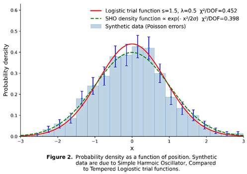
At these initial parameter values, the ${\chi }^2/\mathrm{DOF}$ of the fit is 0.452. Crucially, this value never falls below that of the green dashed curve—representing the true SHO ground-state density—regardless of the parameter values chosen. The optimally fitted version of the trial function coincides exactly with the solid red SHO density curve, as will be discussed later. This specific ansatz allows us to demonstrate how the optimization step(s) may lead to the correct underlying potential even when utilizing a suboptimal trial function. Substituting this baseline trial density into Equation (11) yields the corresponding potential function:

$$V\left(x\right)={\displaystyle \frac{{\mathrm{\hslash }}^2}{2m}}\left[{\lambda }^2{x}^2-\lambda +{\displaystyle \frac{\lambda x}{s}}\tanh \left({\displaystyle \frac{x}{2s}}\right)+{\displaystyle \frac{1}{2s^2}}{\tanh }^2\left({\displaystyle \frac{x}{2s}}\right)-{\displaystyle \frac{1}{4s^2}}\right]+E_0.$$

(43)

While this derived potential is analytically complex, it offers predictive utility as a phenomenological model. Alternatively, a refinement step can be employed to optimize the functional ansatz, aiming to uncover a simpler form, or even the true analytical representation of the system. As suggested by the data in Figure 2, if the empirical distribution indicates that the ground-state motion is localized such that $x\ll s$ for most particle positions, we can expand $\tanh \left({\displaystyle \frac{x}{2s}}\right)$ as a first-order Taylor series for small arguments. This approximation simplifies Equation (43) to:

$$V\left(x\right)={\displaystyle \frac{{\lambda }^2{\hslash }^2}{2m}}{x}^2-{\displaystyle \frac{\lambda {\hslash }^2}{2m}}+E_0.$$

(44)

Within this regime, the complex hybrid potential reduces analytically to a harmonic well plus a physically inconsequential constant energy offset. Furthermore, if the measured energy $E_0$ and the optimized parameter $\lambda$ satisfy the relation:

$$\lambda ={\displaystyle \frac{2m{E}_0}{{\hslash }^2}}$$

(45)

the constant energy offset in (44) is eliminated, yielding the standard potential function:

$$V\left(x\right)={\displaystyle \frac{{\lambda }^2{\hslash }^2}{2m}}{x}^2.$$

(46)

This expression yields the potential under our limiting assumption $x\ll s$. We can now proceed by substituting this potential function into Equation (3) to construct the Hamiltonian, followed by solving the eigenvalue problem in Equation (2) to find the energy eigenvalues and wavefunctions. For this specific case, however, the explicit derivation can be bypassed; the quadratic form of the potential in Equation (46) uniquely specifies a simple harmonic oscillator system with well-established solutions. Consequently, the system possesses the conventional ground-state energy $E_0={\displaystyle \frac{1}{2}}\hslash \omega$. Matching the empirical measurement $E_0$ to this theoretical baseline yields the characteristic frequency $\omega ={\displaystyle \frac{2E_0}{\hslash }}$. Combining this energy condition with Equation (45) yields $\lambda ={\displaystyle \frac{m\omega }{\hslash }}$. To examine the asymptotic behavior of the system, we take the limit $s\to \infty$. Defining the dimensionless variable $u={\displaystyle \frac{x}{s}}$, the trial density function behaves asymptotically as:

$$\rho \left(x\right)\approx N^2{\displaystyle \frac{e^{-u}}{s{\left(1+e^{-u}\right)}^2}}{e}^{-\lambda x^2}\approx {\displaystyle \frac{N^2}{4s}}{e}^{-\lambda x^2}.$$

(47)

In this Equation, absorbing the constant factor ${\displaystyle \frac{1}{4s}}$ into the global normalization constant and substituting our derived expression for $\lambda$, the probability density function reduces to its final asymptotic form:

$$\rho \left(x\right)=N^2{e}^{-{\displaystyle \frac{m\omega }{\hslash }}{x}^2}.$$

(48)

This result is consistent with the exact SHO ground-state wavefunction, ${\psi }_0\left(x\right)=N{e}^{-{\displaystyle \frac{m\omega }{2\hslash }}{x}^2}$, confirming that the exact physical dynamics is recovered. At this point, one would typically fit the ensemble data with this updated functional form to re-evaluate the parameters. However, because Equation (48) contains no remaining free parameters, we directly evaluate its goodness-of-fit to the empirical dataset. This optimized distribution is plotted as the green dashed curve in Figure 2, yielding a ${\chi }^2/\mathrm{DOF}$ of 0.398. Notably, this value remains lower than any fit achievable by the initial trial function in Equation (41), regardless of its parameter choices, matching it only in the formal limit $s\to \infty$. Substituting this refined density from Equation (48) into Equation (11) yields the potential:

$$V\left(x\right)={\displaystyle \frac{1}{2}}m{\omega }^2{x}^2-{\displaystyle \frac{1}{2}}\hslash \omega +E_0.$$

(49)

In this Equation, under the physical condition $E_0={\displaystyle \frac{1}{2}}\mathrm{\hslash }\omega$, the constant terms cancel exactly. This recovers the standard SHO potential $V(x)={\displaystyle \frac{1}{2}}m{\omega }^2{x}^2$, confirming the self-consistency of the framework and utility of refinement step. At this stage, the framework demonstrates the capacity to resolve the exact underlying dynamics, identifying the system explicitly as a simple harmonic oscillator. Applying Equation (7), the complete time-dependent wavefunction is identical to that derived in Equation (26), expressible in terms of standard Hermite polynomials.

A final verification involves evaluating the system in an excited state to compare the measured energy eigenvalues against the theoretical spectrum $E_{\mathrm{n}}=\left(n+{\displaystyle \frac{1}{2}}\right)\mathrm{\hslash }\omega$. Because the energy spacing in an SHO system is uniquely uniform, detecting this constant spectral interval provides a definitive signature to establish the validity of the results.

6. Discussions

The foregoing examples explicitly demonstrate the utility of quantum kinematic techniques in achieving quantum inversion. A central theoretical result of this work is that the potential energy governing a quantum system is uniquely recoverable from its measured probability density alone. This non-trivial result forms the logical foundation upon which all subsequent computational developments rest. By analyzing an uncharacterized physical system via ensemble-based quantum measurements, this framework can successfully uncover the underlying dynamics governing its temporal evolution. Crucially, the proposed kinematical approach offers a promising pathway for discovering quantum interaction laws that might otherwise remain inaccessible, particularly when the driving mechanisms are too intricate to be resolved from first principles.

Our examples show that studying a well-prepared ensemble systematically determines the system's density function—or wavefunction for stationary states. Mechanistically, the framework pairs ground-state position measurements to screen density candidates with excited-state energy measurements to break the deadlock and uniquely isolate the true potential. Resolving these functions subsequently unlocks all primary physical properties unambiguously. To demonstrate its viability under realistic constraints, the framework was evaluated against synthetic position distribution data with explicit error bars, indicating the practicality of the potential reconstruction. Deploying this framework against real-world experimental data will undoubtedly introduce distinct challenges, yet it establishes a baseline for future data-driven quantum discoveries.

A substantial body of existing literature addresses a different domain of quantum inversion, notably compiled in conference proceedings [23]. While those valuable contributions share our objective of identifying quantum dynamics, they typically focus on highly specific, mathematically complex applications restricted to narrow scattering problems. In contrast, our research introduces a broad, generalized framework for direct quantum inversion. Although current implementations serve as a foundational demonstration, this approach establishes a scalable template for future development and broader physical applications. Given this methodological alignment, the terms "kinematical studies" and "quantum inversion" are used interchangeably throughout this text.

Future work will focus on deploying this kinematical framework against empirical density measurements as experimental datasets become available. Additionally, extending the methodology to treat non-stationary states represents a promising avenue for modeling time-dependent density as a source of additional leverage. Because our current implementation utilizes excited-state energies alone—requiring no knowledge of their corresponding wavefunctions or density functions—adapting the framework for hybrid non-stationary ensembles may enhance its predictive potential. Finally, applying these developed concepts to scattering phenomena represents another distinct front, extending the reach of these investigations to non-bounded systems.

7. Conclusions

From a broader epistemological perspective, this framework implicitly questions the convention of discovering physical laws within classical mechanics before exporting their dynamics to the quantum domain. As Examples 1–5 demonstrate, deducing physical laws directly from quantum mechanics from the outset is an entirely viable, inverted approach. When physical laws are uncovered natively within the quantum framework via Equations (10), (11), or (13), they manifest as scalar potential energy functions rather than classical forces, for direct integration into quantum wave equations. Practical deployment of this framework requires its native environment: a pure ensemble of quantum states paired with advanced experimental measurement techniques. Absent empirical datasets, we validated the methodology using synthetic examples.

From a practical standpoint, integrating excited-state energy data is vital because it equips our inversion framework with a reliable means to break the deadlock and select the true physical state from variant density candidates. Intriguingly, while this energy data significantly empowers the predictive search, it is theoretically unnecessary. Because the wavefunction inherently encodes all system information, sufficiently large, high-quality empirical data restricted strictly to particle positions across a pure ensemble can isolate the unique density function to independently yield the governing dynamics. This capability initially appears to mirror classical mechanics, where tracking position data uncovers the complete system dynamics. Yet a subtle distinction remains: the quantum framework isolates the governing dynamics from a single snapshot of the ensemble spread in space; the classical framework requires a chronological history. Symmetrically, for quantum reconstruction, a single photograph frozen in time suffices, while classical inversion demands an entire video.

It is important to note that the parametric optimization methodology described in our kinematical studies relies to some degree on physical intuition to construct appropriate trial density functions. While the framework is computationally predictive—and excited-states energy data will provide additional justification for the choices made—this dependency remains challenging for entirely unknown quantum systems. Consequently, we outline an existing non-parametric fitting approach for such cases in Appendix B. Utilizing this alternative option bypasses global trial functions altogether by computing localized finite-difference fields directly from smoothed experimental data. Such a model-free implementation—driven strictly by the empirical data itself—may be the only solution for handling arbitrary, highly intricate dynamics. While this method relinquishes an explicit analytical expression for the potential, it retains full physical utility; the resulting model-free potential remains entirely accessible for further mathematical operations via localized numerical grids and callable functions.

In a final speculative twist, this study tempts us to imagine a universe where classical mechanics was never needed nor discovered. In such a counterfactual scenario, microscopic intelligent observers—operating on spatial scales inherent to elementary particles—would naturally discover quantum mechanics first, making it their native framework for uncovering physical laws. Absent the classical notion of force, this inversion methodology begins to partially answer how these observers would postulate, explain, and articulate the fundamental laws of nature directly from quantum explorations.

Appendix A.1. General Methods

Using the NLL method to fit a trial probability density function, $\rho \left(x;\overrightarrow{\theta }\right)$, to empirical data involves solving for the optimal free-parameter vector, $\overrightarrow{\theta }$, by minimizing a positive cost function, rather than directly maximizing an unscaled probability density. To account for finite experimental resolution, parameter constraints, and physical boundaries simultaneously, the total cost function is defined as:

$$\begin{array}{l}\mathrm{N}\mathrm{L}\mathrm{L}({\mathcal{N}}_r,\overrightarrow{\theta })=-{\displaystyle \sum _{i=1}^N}\ln {\displaystyle \frac{{\int }_{x_{min}}^{x_{max}}\rho \left(x^{\prime };\overrightarrow{\theta }\right)\cdot \frac{e^{-\frac{{\left(x_i-x^{\prime }\right)}^2}{2{\sigma }_i^2}}}{\sqrt{2\pi }{\sigma }_i}d{x}^{\prime }}{{\mathcal{N}}_r{\int }_{x_{min}}^{x_{max}}\rho \left(x^{\prime };\overrightarrow{\theta }\right)\hspace{0.17em}d{x}^{\prime }}}+{\displaystyle \sum _{k=1}^K}{\displaystyle \frac{{\left[G_k\left(\overrightarrow{\theta }\right)\right]}^2}{2{\sigma }_{G_k}^2}}\\ \hspace{1em}\hspace{1em}\hspace{1em}\hspace{1em}\hspace{1em}+{\displaystyle \sum _{m=1}^M}{\displaystyle \frac{{\left[H_m\left(x;\overrightarrow{\theta }\right)\right]}^2}{2{\sigma }_{H_m}^2}}.\end{array}$$

(A1)

The operational mechanics of Equation (A1) can be divided into three distinct functional contributions [17]:

○

Smearing and Normalization: The first term on the right-hand side processes the raw data points, $x_i$. The numerator models experimental position-measurement limitations by applying a localized Gaussian smearing effect of width ${\sigma }_i$. The corresponding denominator applies a normalization factor, ${\mathcal{N}}_r$, ensuring that the trial distribution integrates to unity across the bounded domain ${[x}_{min},x_{max}]$.

○

Parameter Constraints: The second term introduces a "soft" implementation of a priori constraints acting directly on the parameter values. Here, $G_k\left(\overrightarrow{\theta }\right)$ represents the $k$-th constraint function, penalizing deviations from preferred parameter ranges, scaled by an assigned penalty weight ${\sigma }_{G_k}$.

Appendix A.2. Core Fitting Parameters & Variables

While Negative Log-Likelihood minimization is an established statistical estimation technique, its specific parameterizations within this framework dictate the accuracy and stability of the quantum inversion process. This section defines the primary variables necessary to interpret the statistical optimizations detailed in Section 5.1.1 (Table 1).

○

$x_i$ (Empirical Data Points): Individual, un-binned coordinate measurements (e.g., particle positions) mapped directly within the continuous cost function, completely bypassing the resolution losses associated with histogram binning.

○

$\overrightarrow{\theta }=\left\{{\theta }_1,{\theta }_2,\dots ,{\theta }_k\right\}$ (Free Parameters): The vector of unknown constants within the trial density function, adjusted iteratively by the optimization algorithm to minimize the total NLL.

○

$k$ (Parameter Count): The total number of free degrees of freedom being estimated; minimizing this value balances predictive power against the structural risks of overfitting.

○

$\mathcal{N}$ (Sample Size): The total number of individual empirical observations. Increasing $N$ sharpens the parameter constraints and reduces statistical variance, though it scales the absolute magnitude of the total NLL.

Appendix A.3. Key Goodness-of-Fit Metrics

Evaluating un-binned NLL fits requires relative and absolute statistical measures to judge model efficacy. The primary metrics utilized in Table 1 are defined below:

1. 

Negative Log-Likelihood (NLL) Value

○

Formula: $\mathrm{NLL}=-{\displaystyle {\sum }_{i=1}^N}\ln f\left(x_i;\overrightarrow{\theta }\right)$

○

Description: Quantifies the joint probability density of observing the empirical dataset given the specific parameters of the trial function.

○

Interpretation: Lower (more negative) values indicate a superior fit. Because the absolute NLL scale is relative and dependent on sample size, it cannot evaluate a single model in isolation; instead, it determines which candidate function is statistically favored when evaluated against the same dataset.

2. 

Likelihood Ratio Test / Delta Chi-Squared ($\mathsf{\Delta }\left(-2\ln L\right)$)

○

Formula: $\mathsf{\Delta }\left(-2\ln L\right)=2\left({\mathrm{NLL}}_{\mathrm{model}}-{\mathrm{NLL}}_{\mathrm{best}}\right)$

○

Description: Measures the statistical degradation of a competing trial function relative to the best-performing (lowest NLL) model.

○

Interpretation: For nested models, this difference asymptotically follows a ${\chi }^2$ distribution. A high $\mathsf{\Delta }$ value indicates a statistically significant rejection of the inferior candidate model.

3. 

Akaike Information Criterion (AIC)

○

Formula: $\mathrm{AIC}=2k-2\ln L=2k+2\left(\mathrm{NLL}\right)$

○

Description: Assesses model quality by balancing goodness-of-fit against parameter complexity, adding a penalty of $+2$ for each free parameter $k$.

○

Interpretation: Lower values indicate a preferred model. It prevents overfitting by penalizing the introduction of unnecessary statistical degrees of freedom that fail to yield a corresponding, statistically significant reduction in the baseline NLL.

4. 

Bayesian Information Criterion (BIC)

○

Formula: $\mathrm{BIC}=k\ln \left(\mathcal{N}\right)-2\ln L=k\ln \left(\mathcal{N}\right)+2\left(\mathrm{NLL}\right)$

○

Description: Like the AIC but scales the complexity penalty relative to the total dataset size ($\ln \mathcal{N}$).

○

Interpretation: Lower values indicate a preferred model. For datasets where $\mathcal{N}>7$, the BIC penalizes additional free parameters more aggressively than the AIC, strongly favoring parsimonious functional forms.

5. 

Kolmogorov-Smirnov (KS) Test$p$ -value

○

Method: A bin-free metric that compares the empirical Cumulative Distribution Function (CDF) of the data directly against the optimized model's theoretical CDF by identifying the maximum vertical distance ($D$) between the two curves.

○

Interpretation: Yields an absolute probability ($p$-value). A high $p$-value ($p>0.05$) indicates that the optimized model is statistically consistent with the underlying data distribution. Conversely, a low $p$-value ($p<0.05$) rejects the trial function as an improper description of the system dynamics.

Appendix A.4. Binned Chi-Squared over Degrees of Freedom (${\chi }^2/\mathit{DOF}$)

○

Method: Although the primary optimization relies on an un-binned continuous NLL method, the experimental data can be grouped post-fit into discrete histogram bins. This allows for the calculation of a traditional ${\chi }^2$ statistic against the integrated model curve across the binned intervals.

○

Interpretation:

• ${\chi }^2/\mathrm{DOF}\approx 1$: Indicates an optimal fit where model deviations align precisely with expected statistical fluctuations.
• ${\chi }^2/\mathrm{DOF}\gg 1$: Indicates a poor fit, signaling that the chosen trial function systematically fails to resolve the structural geography of the data.
• ${\chi }^2/\mathrm{DOF}\ll 1$: Indicates that the model is either overfitting statistical noise or that the experimental variance parameters are fundamentally overestimated.

Appendix A.5. Multi-Metric Fit Evaluation Matrix

When evaluating and competing multiple trial functions—such as a fixed parabolic model $f\left(x\right)$, a constrained integer polynomial $g\left(x\right)$, and a highly flexible trigonometric model $h\left(x\right)$—establishing an objective conclusion requires multi-metric agreement. The decision thresholds are codified below:

Table A1. Explanation of NLL Metrics.

Metric Behavior	Interpretation	Action
Lowest NLL, AIC, BIC High KS p-value > 0.05 ${\chi }^2/\mathrm{DOF}\approx 1$	Model is highly favored, mathematically stable, and physically viable.	Accept trial function as a valid inversion candidate.
Elevated NLL, AIC, BIC $\mathrm{KS} p$$-\mathrm{value} < 0.05$ ${\chi }^2/\mathrm{DOF}>2.0$	Model fails both binned and bin-free structural tests due to geometric rigidity.	Reject trial function; the model ansatz is structurally excluded.
Favorable AIC/BIC $\mathrm{Borderline} \mathrm{KS} p$$-\mathrm{value} \approx 0.06$ $\mathrm{Marginal} {\chi }^2/\mathrm{DOF}$ balance	Model captures global geometric trends but fails at boundary constraints or tails.	Execute power analysis; $\mathrm{collect} \mathrm{higher} \mathrm{density} \mathrm{datasets} (N$) to test rejection limits.

Table A1. Explanation of NLL Metrics.

Metric Behavior	Interpretation	Action
Lowest NLL, AIC, BIC High KS p-value > 0.05 ${\chi }^2/\mathrm{DOF}\approx 1$	Model is highly favored, mathematically stable, and physically viable.	Accept trial function as a valid inversion candidate.
Elevated NLL, AIC, BIC $\mathrm{KS} p$$-\mathrm{value} < 0.05$ ${\chi }^2/\mathrm{DOF}>2.0$	Model fails both binned and bin-free structural tests due to geometric rigidity.	Reject trial function; the model ansatz is structurally excluded.
Favorable AIC/BIC $\mathrm{Borderline} \mathrm{KS} p$$-\mathrm{value} \approx 0.06$ $\mathrm{Marginal} {\chi }^2/\mathrm{DOF}$ balance	Model captures global geometric trends but fails at boundary constraints or tails.	Execute power analysis; $\mathrm{collect} \mathrm{higher} \mathrm{density} \mathrm{datasets} (N$) to test rejection limits.

Appendix A.6. Synthetic Data Simulation Framework

To validate the computational stability of this optimization pipeline, an un-binned NLL fit was executed on a controlled synthetic dataset to calculate the full spectrum of goodness-of-fit metrics. Synthetic coordinates are sampled from an underlying, asymmetric Beta-like distribution and optimized using the following normalized parametric ansatz:

$$\rho \left(x\right)={\displaystyle \frac{x^a{\left(1-x\right)}^b}{\mathcal{B}\left(a+1,b+1\right)}}$$

(A2)

where function $\mathcal{B}$ represents the Euler Beta function, acting as an intrinsic, parameter-dependent normalization factor across the boundary domain with boundaries at $x=\mathrm{0,1}$ where $\rho \left(x\right)$ vanishes as a particle in a box would. The graphical results for the data distribution and the corresponding best-fit curve from Equation (A2) are displayed in Figure A1 as points with error bars and a solid blue line, respectively.

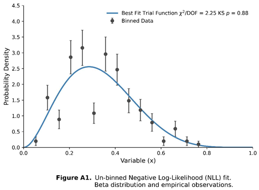
Complementing the visual validation by Figure A1, Table A2 below details the optimized parameter values and goodness-of-fit metrics quantifying the performance of the minimization pipeline. Based on the established validation criteria, both the statistical metrics and the visual alignment in Figure A1 confirm that the parametric trial function delivers a highly accurate description of the underlying distribution.

Table A2. Fit Summary: Example Metrics.

Optimization Parameter / Metric	Numerical Output	Statistical Characterization & Threshold Criteria
$\mathbf{Optimized} \mathbf{Parameter} a$	2.011	$\mathrm{Convergence} \mathrm{tracks} \mathrm{the} \mathrm{true} \mathrm{generating} \mathrm{coordinate} \mathrm{distribution} (a_{\mathrm{true}}=2.0$).
$\mathbf{Optimized} \mathbf{Parameter} b$	5.032	$\mathrm{Convergence} \mathrm{tracks} \mathrm{the} \mathrm{true} \mathrm{generating} \mathrm{coordinate} \mathrm{distribution} (b_{\mathrm{true}}=5.0$).
Minimum NLL Value	-103.585	Establishes the localized global minimum for the continuous dataset.
Akaike Information Criterion (AIC)	-203.170	$\mathrm{Baseline} \mathrm{informational} \mathrm{score} \mathrm{optimized} \mathrm{for} \mathrm{a} \mathrm{parameter} \mathrm{count} \mathrm{of} k=2$.
Bayesian Information Criterion (BIC)	-196.573	Confirms parsimony relative to the total continuous sample volume.
Kolmogorov-Smirnov (KS) p-value	0.8800	$\mathrm{High} \mathrm{confidence} (p\gg 0.05$); fails to reject the continuous model ansatz.
Binned χ²/DOF	2.253	Structural variance profiling post-binning; baseline noise validation indicator.

Table A2. Fit Summary: Example Metrics.

Optimization Parameter / Metric	Numerical Output	Statistical Characterization & Threshold Criteria
$\mathbf{Optimized} \mathbf{Parameter} a$	2.011	$\mathrm{Convergence} \mathrm{tracks} \mathrm{the} \mathrm{true} \mathrm{generating} \mathrm{coordinate} \mathrm{distribution} (a_{\mathrm{true}}=2.0$).
$\mathbf{Optimized} \mathbf{Parameter} b$	5.032	$\mathrm{Convergence} \mathrm{tracks} \mathrm{the} \mathrm{true} \mathrm{generating} \mathrm{coordinate} \mathrm{distribution} (b_{\mathrm{true}}=5.0$).
Minimum NLL Value	-103.585	Establishes the localized global minimum for the continuous dataset.
Akaike Information Criterion (AIC)	-203.170	$\mathrm{Baseline} \mathrm{informational} \mathrm{score} \mathrm{optimized} \mathrm{for} \mathrm{a} \mathrm{parameter} \mathrm{count} \mathrm{of} k=2$.
Bayesian Information Criterion (BIC)	-196.573	Confirms parsimony relative to the total continuous sample volume.
Kolmogorov-Smirnov (KS) p-value	0.8800	$\mathrm{High} \mathrm{confidence} (p\gg 0.05$); fails to reject the continuous model ansatz.
Binned χ²/DOF	2.253	Structural variance profiling post-binning; baseline noise validation indicator.

Methodological Interpretation of Validation of the Fit Outputs:

• Parameter Convergence Dynamics: The optimized shape coefficients ($a=2.011$, $b=5.032$) converge tightly around the true underlying generating integers (2.0, 5.0). This highly localized convergence demonstrates the mathematical inversion pipeline's structural stability and numerical accuracy in extracting coordinate dynamics.
• Continuous Boundary Verification via KS Test: Because the trial functional ansatz aligns precisely with the underlying continuous physical distribution shape, the empirical cumulative distribution function matches the theoretical model. The resulting $p-value$ settles comfortably above the critical rejection threshold ($0.8800\gg 0.05$), statistically validating that the inverted model cannot be rejected as an improper description of the system.
• Binned Residual Variances: The post-fit binned $\chi ²/DOF$ profile targets the expected baseline region. This proximity to unity signals that the residual variances between the empirical coordinate histogram bins and the continuous parametric inversion curve are driven by expected statistical noise rather than geometric model bias.

Appendix A.7. The Mathematics of Minimization Under Continuous Constraints

When transitioning from discrete data optimizations to enforcing a continuous physical property across an entire coordinate space x, the soft penalty term mathematically transforms from a discrete summation into a definite functional integral. This section outlines the analytical architecture of these continuous regularizers.

The Total Objective Function:

When minimizing the Negative Log-Likelihood subject to a continuous penalty, the total objective cost function $C\left(\overrightarrow{\theta }\right)$ is defined as:

$$C\left(\overrightarrow{\theta }\right)={\mathrm{NLL}}_{\mathrm{base}}\left(\overrightarrow{\theta }\right)+{\mathcal{L}}_{\mathrm{penalty}}\left(\overrightarrow{\theta }\right)$$

$${\mathrm{NLL}}_{\mathrm{base}}\left(\overrightarrow{\theta }\right)=-{\displaystyle \sum _{i=1}^N}\ln f\left(x_i;\hspace{0.17em}\overrightarrow{\theta }\right) .$$

The Soft Penalty Integral Architectures:

To systematically enforce target physical behaviors or boundary constraints across a continuous domain, the penalty contribution ${\mathcal{L}}_{\mathrm{penalty}}\left(\overrightarrow{\theta }\right)$ utilizes a definite integral evaluated over the physical boundary interval $\left[0,L\right]$ or $\left[a,b\right]$. Within this optimization framework, the arbitrary multiplier λ is replaced by an explicit, user-defined inverse variance parameter to establish a mathematically rigorous soft constraint, as structurally modeled in Equation A1.

Case A: General Equality Constraints (G(x) = 0)

If a specific physical property must hold uniformly across all spatial positions $x$, the localized functional violation is squared and integrated over the continuous domain to form a global regularizer:

$${\mathcal{L}}_{\mathrm{penalty}}\left(\overrightarrow{\theta }\right)=\lambda {\int }_0^L{\left[G\left(x;\overrightarrow{\theta }\right)\right]}^{2}dx.$$

Example: Normalization Enforced via Continuous Penalty.

To systematically compel an unnormalized trial function $f\left(x;\overrightarrow{\theta }\right)$ to integrate to unity across the bounded space, the global normalization deviation is squared and penalized:

$${\mathcal{L}}_{\mathrm{norm}}\left(\overrightarrow{\theta }\right)=\lambda {\left({\int }_0^{L}f\left(x;\overrightarrow{\theta }\right)\hspace{0.17em}dx-1\right)}^2.$$

Case B: Global Inequality Constraints ($G\left(x\right)\ge 0$)

When a constraint must only trigger if a continuous function violates a specific physical threshold—such as preventing a spatial probability density from dropping into unphysical negative regimes ( $f\left(x\right)<0$)—the framework utilizes a clipped hinge loss or Rectified Linear Unit (ReLU)-style conditional boundary inside the functional integral:

$${\mathcal{L}}_{\mathrm{ineq}}\left(\overrightarrow{\theta }\right)=\lambda {\int }_0^L{\left[\min \left(0,G\left(x;\overrightarrow{\theta }\right))\right)\right]}^{2}dx.$$

Mechanical Interpretation: If the underlying condition $G\left(x;\overrightarrow{\theta }\right)\ge 0$ is satisfied across all coordinates, the localized conditional term evaluates identically to zero and contributes nothing to the objective cost. Conversely, if the distribution drops below zero, the localized functional violation is squared, integrated continuously over all spatial sub-regions where the threshold failed, and scaled by the penalty weight $\lambda$.

Case C: Smoothness and Curvature Regularization

To minimize unphysical, high-frequency oscillations (wiggling) within the trial model and suppress over-fitting, a regularizer penalizes the squared second spatial derivative across the entire continuous domain:

$${\mathcal{L}}_{\mathrm{smooth}}\left(\theta \right)=\lambda {\int }_0^L{\left[f\prime \prime \left(x;\theta \right)\right]}^{2}dx.$$

Numerical Quadrature Schemes for Arbitrary Trial Functions: Because analytical solutions for these continuous integrals are rarely obtainable for arbitrary, highly non-linear trial functions, the functional expressions are evaluated computationally over a uniform grid using standard numerical quadrature rules (e.g., the Midpoint rule or Simpson's rule):

$${\int }_0^{L}V\left(x\right)\hspace{0.17em}dx\approx {\displaystyle \sum _{j=1}^M}V\left(x_j\right)\cdot \mathsf{\Delta }x$$

where $M$ represents a fine grid of static evaluation points (typically $M=500$ steps) completely decoupled from the $N$ un-binned empirical data coordinates. This exact grid architecture allows isolated global point penalties—such as fixed-point boundary constraints like $G\left(0\right)=0$—to be integrated directly into the total penalty landscape.

Appendix A.8. Comparative Analysis: Un-binned NLL vs. Binned χ² Minimization

The Negative Log-Likelihood optimization framework differs fundamentally from the traditional $\chi ²$ minimization approach in its data handling, structural flexibility, and constraint integration. The $\chi ²$ method relies on grouping continuous data into discrete histogram intervals, optimizing parameters against the binned counts via the definition:

$${\chi }^2={\displaystyle \sum _{j=1}^{N_{bins}}}{\displaystyle \frac{{\left(N_j-n_j\left(\overrightarrow{\theta }\right)\right)}^2}{N_j}}$$

(A2)

where $N_j$ represents the observed empirical particle count in bin j, and $n_j\left(\overrightarrow{\theta }\right)$ denotes the expected count predicted by integrating the candidate probability density function over that specific bin interval:

$$n_j\left(\overrightarrow{\theta }\right)=N{\int }_{x_j}^{x_{j+1}}\rho \left(x;\hspace{0.17em}\overrightarrow{\theta }\right)\hspace{0.17em}dx.$$

This formulation implicitly assumes Poisson-weighted statistical uncertainties (${\sigma }_j=\sqrt{N_j}$) for each bin count, evaluating model viability over the total degrees of freedom defined by $\mathrm{DOF}=N_{\mathrm{bins}}-k-1$, where $k$ is the number of free parameters.

Structural Contrast and Constraint Implementation

The critical operational distinctions between the two methodologies are summarized below:

• Algorithmic Architecture: The continuous, un-binned NLL formulation in Equation (A1) features intrinsic mathematical provisions to handle normalization scaling (${\mathcal{N}}_r$), global parameter constraints ($G_k$), and localized physical boundary conditions ($H_m$) simultaneously within a single objective function.
• Mathematical Constraints: Conversely, the standard χ² objective function in Equation (A10) is not natively equipped to process soft regularizers or continuous boundary integrals. To enforce physical boundary states or normalization invariants within a χ² pipeline, the researcher must analytically hard-code these constraints directly into the trial function's algebraic formulation beforehand (as demonstrated by the boundary-locked polynomial derivation in Section B.2).
• Resolution and Bias: While the un-binned NLL method extracts dynamics from individual coordinate entries without losing spatial information, the χ² method introduces artificial geometric bias based entirely on the selection of bin widths and boundary placement, making the NLL approach more robust for reconstructing highly localized or asymmetric quantum potentials.

While the parametric NLL framework detailed in this Appendix provides an optimization pathway when an underlying geometric form can be accurately anticipated, its success remains bound to the physical intuition used to construct the trial ansatz. To address scenarios involving entirely unknown or highly intricate quantum states where such structural assumptions inevitably break down, Appendix B outlines an alternative, ansatz-free non-parametric methodology driven strictly by localized empirical data.

Appendix B.1. Empirical Data Simulation Mechanics

To rigorously evaluate the inversion pipeline under realistic laboratory constraints, experimental data is simulated via discrete coordinate sampling rather than idealized smooth distributions. Individual particle position coordinates $x_i$ are sampled from a known asymmetric double-well ground-state probability distribution using a stochastic acceptance-rejection framework. To avoid the unphysical step discontinuities and localized derivative spikes inherent in standard histograms, a continuous empirical density profile is reconstructed directly from $\mathcal{N}$ discrete positional events using Kernel Density Estimation (KDE) [12,13]:

$${\rho }_{\mathrm{KDE}}\left(x\right)={\displaystyle \frac{1}{Nb}}{\displaystyle \sum _{i=1}^{\mathcal{N}}}K\left({\displaystyle \frac{x-x_i}{b}}\right)$$

(B1)

where $K$ represents a standard Gaussian kernel envelope, and $b$ denotes the optimization bandwidth.

Sparse local observations are extracted at twenty-five discrete spatial points across the box interval $\left[0,L\right]$. To emulate fundamental quantum measurement uncertainties, localized vertical error bars ${\sigma }_i$ are applied to each point using standard Poisson counting statistics (${\sigma }_i\propto \sqrt{N_i}$). This variable uncertainty forces the error boundaries to swell near high-amplitude peaks while tracking tightly to zero as the coordinates approach the absolute walls of the box where the probability vanishes.

Appendix B.2. Derivation of the Boundary-Locked Polynomial Ansatz

To demonstrate the limitations of classical guess-based parametric modeling, a rigid trial function baseline was constructed using a 4th-degree polynomial:

$${\rho }_{\mathrm{ansatz}}\left(x\right)=a{x}^4+b{x}^3+c{x}^2+dx+e.$$

For this function to remain physically valid for a quantum particle trapped inside an infinite 1D box of length $L=1$, it must simultaneously satisfy three strict boundary and normalization invariants:

• Left Wall Boundary Condition: $\rho \left(0\right)=0⟹e=0$
• Right Wall Boundary Condition: $\rho \left(1\right)=0⟹a+b+c+d=0$
• Total Probability Normalization: ${\int }_0^1\rho \left(x\right)dx=1⟹{\displaystyle \frac{a}{5}}+{\displaystyle \frac{b}{4}}+{\displaystyle \frac{c}{3}}+{\displaystyle \frac{d}{2}}=1$

Solving this linear system of equations eliminates two degrees of freedom, pinning the remaining dependent coefficients ($c$ and $d$) analytically to the free shape parameters $a$ and $b$:

$$c=-1.8a-1.5b-6.0$$

$$d=0.8a+0.5b+6.0.$$

The resulting boundary-locked, normalized parametric trial function becomes:

$${\rho }_{\mathrm{ansatz}}\left(x\right)=a{x}^4+b{x}^3-\left(1.8a+1.5b+6.0\right)x^2+\left(0.8a+0.5b+6.0\right)x.$$

Appendix B.3. Parametric Rigidity vs Non-Parametric Necessity

The structural performance of this boundary-locked ansatz is visualized in Figure B1, with its shape parameters optimized via a Poisson-weighted Chi-squared ($\chi ²$) minimization over the simulated coordinate data. At its absolute mathematical optimum ($a=12.50$, $b=-12.50$), the parametric curve fails to resolve the underlying physical landscape. Because a single global polynomial is structurally too rigid to accommodate multi-modal variations, the optimization routine gets trapped in a severe geometric compromise: the curve flattens out into a single wide lobe, bridging directly over the central tunneling valley while truncating both local density peaks. Attempting to resolve this structural rigidity by advancing to a 5th-degree polynomial yields negligible improvements; instead, the additional degree of freedom triggers unphysical edge oscillations near the boundaries—a manifestation of Runge's phenomenon—without resolving the internal dual-well geography.

Conversely, ansatz-free non-parametric fitting methods resolve the asymmetric double-hump configuration with complete fidelity. As shown in Figure B1, a Gaussian kernel approach yields a smooth, continuous, and infinitely differentiable field, passing data directly into numerical calculus engines. Alternatively, a localized cubic B-spline kernel can be applied to achieve indistinguishable structural results; the B-spline method offers enhanced computational speed for large datasets, whereas the Gaussian kernel guarantees the clean calculation of higher-order derivatives.

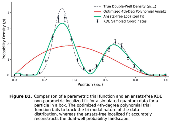
Operating free from predefined global geometric constraints, these non-parametric fits safely suppress localized statistical noise spikes while tracking the sharp rise of the primary peak, the deep descent of the tunneling barrier valley, and the localized curvature of the secondary peak. This explicit operational divergence demonstrates that when global geometric models are inadequate, non-parametric approaches offer a physically bounded and mathematically rigorous framework for reconstructing completely unknown quantum systems. While this method relinquishes a closed-form analytical expression for the potential, it retains full physical utility; the resulting potential remains entirely accessible for further mathematical operations via localized numerical grids, Fourier transforms, or callable functions within Hilbert space.

References

- Planck, M. Ueber das Gesetz der Energieverteilung im Normalspectrum. Ann. Der Phys. 1901, 4, 553–563. [Google Scholar] [CrossRef]
- Rydberg, J. Recherches sur la constitution des spectres d'émission des éléments chimiques. K. Sven. Vetenskapsakad. Handl. 1890, 23, 1–155. [Google Scholar]
- Ritz, W. Über ein neues Gesetz der Serienspektren (On a new law of series spectra). Phys. Z. 1908, 9, 521–529. [Google Scholar]
- Bohr, N. On the Constitution of Atoms and Molecules. Philos. Mag. J. Sci. 1913, 26(151), 1–24. [Google Scholar] [CrossRef]
- Sommerfeld, A. Zur Theorie der Balmerschen Serie. Sitzungsberichte Der Königlich Bayer. Akad. Der Wiss. Zu München 1915, 425–458. [Google Scholar]
- de Broglie, L. Recherches sur la théorie des Quanta. Ann. Phys. 1925, 10, 22–128. [Google Scholar] [CrossRef]
- Heisenberg, W. Über quantentheoretische Umdeutung kinematischer und mechanischer Beziehungen. Z. Phys. 1925, 33, 879–893. [Google Scholar] [CrossRef]
- Schrödinger, E. Quamtisierung als Eignwertproblem. Ann. Phys. 1926, 384, 361–376. [Google Scholar]
- Einstein, A. Zur Quantentheorie der Strahlung [On the quantum theory of radiation]. Phys. Z. 1917, 18, 121–128. [Google Scholar]
- Silverman, B.W. Density Estimation for Statistics and Data Analysis; Chapman & Hall: London – New York: New York, NY, USA, 1986. [Google Scholar]
- Lenk, P.; Lee, J.; Han, D.; Park, J.; Choi, T. Hierarchical Bayesian spectral regression with shape constraints for multi-group analysis. Comput. Stat. Data Anal. 2024, 200, 108036. [Google Scholar] [CrossRef]
- Burbano-Moreno, M. V. Gaussian modeling with B-splines for spatial functional data on irregular domains; Taylor & Francis Online, Statistics, 2024; p. 58. [Google Scholar]
- de Boor, C. A Practical Guide to Splines; Springer: New York, NY, 1978. [Google Scholar]
- Gottfried, K.; Yan, T.M. Quantum Mechanics: Fundamentals, 2nd ed.; Springer: New York, NY, USA, 2004. [Google Scholar]
- Sakurai, J. J.; Napolitano, J. Modern Quantum Mechanics; Cambridge University Press: Cambridge, UK, 2021. [Google Scholar]
- Cowan, G. Statistical Data Analysis in Particle Physics; Oxford University Press: UK, 1998. [Google Scholar]
- Parzen, E. On Estimation of a Probability Density Function and Mode. Ann. Math. Stat. 1962, 33, 832–837. [Google Scholar] [CrossRef]
- Cooper, F.; Khare, A.; &; Sukhatme, U. Supersymetry in Quantum Mechanics; World Scientific: USA-UK, 2001. [Google Scholar]
- Fernandez, C. D. J. Trends in Supersymmetric Quantum Mechanics; Springer New York, NY, USA, 2010. [Google Scholar]
- Bevington, P. R.; Robinson, D.K. Data Reduction and Error Analysis for the Physical Sciences, 3rd ed.; McGraw-Hill: New York, NY, USA, 2003. [Google Scholar]
- Ronveaux, A. Heun's Differential Equations; Oxford Science Publications: Oxford University Press: Oxford, UK, 1995. [Google Scholar]
- Pöschl, G.; Teller, E. Bemerkungen zur Quantenmechanik des anharmonischen Oszillators. Z. Für Phys. 1933, 83, 143–151. [Google Scholar] [CrossRef]
- Geramb, H. V. Quantum Inversion Theory and Applications. Proceedings of 109th W.E. Heraeus Seminar on Quantum Inversion Theory and Applications, Bad Honnet, Germany, 17–19 May 1993. [Google Scholar]