

Submitted:
13 August 2026
Posted:
17 August 2026
You are already at the latest version
Abstract
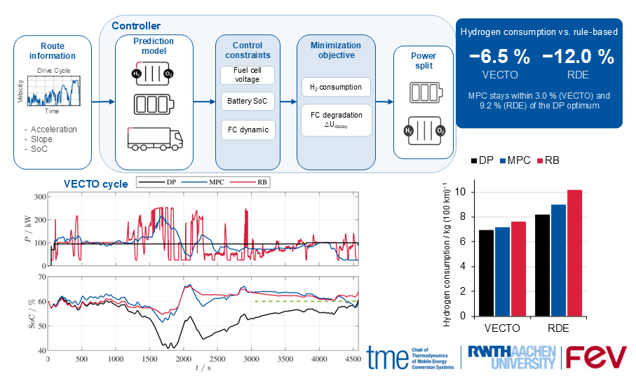
This work presents a model predictive control (MPC) approach for optimizing the powertrain system efficiency of a fuel cell electric heavy-duty vehicle. The MPC determines the power split between the high-voltage traction battery and the fuel cell system so that the power demand of the drive cycle is met, while a second objective extends the lifetime of the fuel cell stack by including stack degradation in the cost function. Based on driving profile information, the controller adjusts the fuel cell power trajectory within a specified prediction horizon such that a target state of charge of the traction battery is reached at the end of the time-discrete horizon, fuel consumption is minimized and excessive degradation is avoided. The control variables are computed from discrete-time models of the fuel cell, the truck and the battery. The resulting non-linear optimization problem is solved with the open-source software package acados, integrated into MATLAB Simulink to achieve real-time capability. The MPC is implemented and tested in a model-in-the-loop environment. On the VECTO Long Haul cycle, hydrogen consumption is reduced by 6.5%, while membrane thinning and the loss of electrochemically active surface area are reduced by 6.1% and 2.3%, respectively, compared with a rule-based strategy.
Keywords:
energy management strategy
; model predictive control
; fuel cell system
; degradation
; heavy-duty vehicle
; hydrogen consumption
; state of health
1. Introduction and Motivation
In order to comply with the maximum global temperature increase of 2 K by 2050 set by the Paris Climate Agreement in 2015, the European Union (EU) has formulated greenhouse gas emission limits for the transportation sector [1]. Based on 2016 data, heavy-duty commercial vehicles are responsible for 27 % of emissions from road transport and around 5 % of greenhouse gas emissions in the EU, according to a press release from the European Parliament [2]. This is due to the increase in freight transport since 1990, which has increased CO2-emissions from heavy-duty vehicles by 25 %. Electric powertrain architectures offer a future-proof solution for meeting greenhouse gas emissions regulations in all possible transport sectors [3]. The transition from fossil fuels to environmentally friendly energy sources introduces new challenges that must be addressed to meet consumer and regulatory demands.
In addition to electrified powertrains, so-called electric vehicles (EVs), fuel cell electric vehicles (FCEVs) in particular offer a promising solution in terms of zero local CO2-emissions, higher energy density and faster recharging compared to battery electric vehicles [3,4]. The reduction of greenhouse gas emissions can be achieved through the integration of a fuel cell and green hydrogen [5] within a powertrain application. In an all-electric FCEV, the fuel cell is the primary energy source [6]. With more than one energy source, a FCEV uses a combination of a fuel cell system and an energy storage system (ESS), preferably a HV traction battery or supercapacitors (SC), to compensate for the slow dynamics of the fuel cell during load changes and to enable the regenerative recovery of braking energy [6,7]. It is evident that fuel cell systems represent a viable option for achieving CO2-neutral mobility, particularly in the context of heavy-duty vehicles [8]. In order to operate a hybrid system with multiple energy sources in an efficient way, an active energy management strategy (EMS) is required. In the case of fuel cell operation, the power distribution must be optimized to operate at the most efficient point, taken into account system constraints and durability [3,4].
1.1. Energy Management Strategies
EMS are operating strategies that attempt to efficiently meet various powertrain requirements, taking into account the optimal use of multiple energy sources. EMS are used to improve the performance of hybrid vehicles in terms of both energy consumption and component lifetime [7].
EMSs can be classified into three groups: rule-based, optimization-based and learning-based EMS. The proposed methods have their own advantages and limitations, which are discussed individually in the following section. Figure 1 provides an overview of the most frequently used optimization algorithms, classified according to their real-time capability and their potential for optimization over the prediction horizon.
To reduce the load change rate of the fuel cell system [9] used a series fuzzy control strategy. As a result, the load changing rate is reduced and limited to the range of change capacity. Fuzzy-logic (FL) control is an extension of conventional rule-based (RB) control based on if-else conditions that attempt to recreate the human decision-making process [10]. Another type of RB-EMS is frequency decoupling, which splits the power demand in the frequency domain so that the high-frequency demand is met by the battery and the low-frequency demand is met by the fuel cell [9,11]. This method has been extended by [12] with an optimization-based strategy to consider not only the dynamic requirements but also the energy efficiency in terms of fuel consumption and state of charge (SoC) management.
Rule-based strategies can be implemented with little effort, since they require neither a plant model nor training data, and their rules can operate on both directly measured and model-based signals. They have a low computation time due to the stationary control decisions based on the input values. However, the heuristic strategies require a high calibration effort in order to guarantee a performance close to optimality for each driving cycle. In addition, the rules are not easily scalable to different powertrain architectures or different component sizes [13].
Learning-based (LB) EMS use data mining methods that utilize historical and real-time information from large amounts of data to derive the optimal control law.
An intelligent energy management concept that employs training data to determine the best power control for a hybrid vehicle system with three or more energy sources and significant load fluctuations is presented in [14]. The machine learning algorithm covers a wide range of power requirements with restrictions in terms of system voltage and keeping the states of charge of the energy storage units within predefined thresholds. By optimally combining the energy sources, the power losses of the overall system were reduced by 28 % up to 76 % compared to a conventional rule based power control [14].
Reinforcement learning (RL) is presented in [15], taking into account the lifetime of the fuel cell system. The RL algorithm is pre-initialized by energy allocation rules to speed up the optimization process. Simulation results show that the average H2 consumption difference between the proposed EMS and a EMS based on DP is 5.59 % in the training and validation driving cycles. In addition, the proposed EMS reduces average power difference of the FCS, which should also reduce the performance degradation. Compared to a conventional RL-based EMS, which does not take into account the lifetime of the fuel cell system, the power fluctuations could be reduced by at least 13 %. This is a significant advantage for improving the lifetime of the fuel cell system.
The learning-based strategies using the example of RL require a large amount of historical data for the development of control strategies and are correspondingly computationally intensive [7,16]. They provide a solution close to optimality and are particularly suitable for multicriteria optimization problems [16]. However, LB strategies based on deep neural networks, such as RL, operate as so-called black box models: the internal decision-making process of the trained network is non-transparent and cannot be formally verified or traced back to physical quantities by engineers [17]. This inherent opacity is fundamentally incompatible with automotive functional safety standards such as ISO 26262, which require formal verification and requirement traceability for safety-critical software in series production vehicle control units [18]. Consequently, LB-based EMS are currently not applicable for series production control units.
Optimization-based (OB) algorithms regulate the control variables based on numerical computation results by minimizing a predefined cost function with feasible constraints [19]. According to [7], Dynamic Programming (DP) and Pontryagin’s Minimum Principle (PMP) are the most frequently used global optimization algorithms. In [20], the DP for a FCEV is used to optimize the fuel cell power to reduce hydrogen consumption and extend the lifetime of the fuel cell. An optimal power distribution strategy for different degradation stages of fuel cells was derived in [21] using DP. Compared to a rule-based strategy, the operating costs of the fuel cell were reduced by 14.17 % and the average lifetime was increased by 8.48 %.
In [22] a health-conscious two stage predictive energy management strategy for fuel cell electric heavy-duty long-haul trucks is proposed to overcome the challenges of durability and efficiency. The multi-objective optimization problem integrates component degradation as an inherit part of the optimization process to reduce the degradation of the battery and the fuel cell taking into account the performance deterioration due to the progressive degradation of the powertrain components. To do so in the first stage the fuel cell power and SoC profiles are optimized for the entire route once at the beginning of the driving cycle. The optimized references are followed by an on-board controller, representing the second stage of the predictive EMS which is based on DP as an online EMS developed in [23].
For a FC vehicle [24] combined an optimal control using the PMP with a Markov chain model. The Markov chain prediction model was used to predict the future energy demand during the driving cycle. Another study used PMP as a global optimization method for the power distribution between the fuel cell and energy storage system in order to minimize hydrogen consumption [25]. Using a developed degradation model, a factor for limiting the fuel cell’s power fluctuations with a weight coefficient was added to the PMP in [26] to increase the lifetime of the fuel cell. In comparison to a RB strategy, simulation results show a reduction of the fuel cell degradation by 56.4 % in the China_city driving cycle respectively 57.8 % in the Highway fuel economy test (HWFET) driving cycle. A similar strategy was used in [27] to limit fuel cell power fluctuations, extended by a SoC range limitation between 40 % and 80 %. As a result, dynamics of the fuel cell output could be reduced by 38.3 % compared to a rule-based strategy.
OB-EMSs such as DP and PMP are able to find a global optimum for the given problem. The DP achieves the highest degree of optimality, but requires the highest computational effort and the longest computing time. The PMP approach can find a comparable optimum with a significantly lower computational cost. However, both strategies are mostly implemented offline due to higher computation requirements. Therefore, local optimization algorithms are primarily the focus for online implementation as shown in [16,28].
Local optimization algorithms such as the Equivalent Consumption Minimization Strategy (ECMS), as well as Model Predictive Control (MPC) and stochastic dynamic programming (SDP), can find a local optimality close to the global optimal solution and can be implemented as real-time applications on control units.
The Equivalent Consumption Minimization Strategy (ECMS) is an online adaptation of the PMP algorithm where the global optimization problem is converted into a local problem.
Fuel consumption is specified as the optimization target in [29]. The total costs are made up of the equivalent cost of hydrogen consumption and the equivalent cost of the battery’s electricity consumption. Since the driving profile is not known in advance, an equivalence factor correction function is used to adjust the SoC of the battery. Here, the actual equivalent factor is calculated by multiplying the SoC correction function by the nominal equivalence factor. In [13], a two-stage ECMS is used to minimize the hydrogen consumption while protecting the PEMFC at the same time. For this purpose in the first stage, a predictive controller is developed using the telemetry equivalent consumption minimization strategy (T-ECMS) approach, which predicts the global optimality trend of the battery state of charge and the local control reference using telemetric driving information data. In the second step, a tracking controller is used that tracks the local control reference in the current control step to follow the optimal SoC reference, taking into account the PEMFC state constraints and other physical constraints. With the advancements in the availability of real-time information [19] presents a multi-layer predictive energy management with a ECMS in the lower layer combined with information such as live traffic data to reduce the fuel consumption. The proposed algorithm leads to a reduced fuel consumption in comparison to a RB strategy for a selected real-world use-case by 7.5 %.
ECMS can be easily implemented in real-time applications but have a lower adaptability for a fixed equivalence factor (EF). Their optimality is strongly dependent on the choice of EF and does not guarantee global optimality [16]. Adaptive ECMS (A-ECMS) can be used for online EF adaptation, providing local optimal solutions in real-time [30]. The real-time adaptation increases the complexity and thus the computing effort of the ECMS.
Model Predictive Control (MPC), also called Receding Horizon Control (RHC), is a global optimization algorithm that is applied as an online method for a finite time interval into the future, called the prediction horizon.
An EMS based on a linear MPC has been developed in [31] to improve battery performance and prevent fuel cell and battery degradation. Taking into account the different operating modes of the battery and the time constraints associated with the activation and deactivation of the fuel cell, an effort is made to maintain the discharge level of the battery at the optimal performance threshold and to minimize the hydrogen consumption. In order to reduce hydrogen consumption and improve the performance of the hybrid vehicle, [32] developed an MPC as a nonlinear constraint optimization problem to predict the optimal power of the fuel cell system in conjunction with prediction models for the future demand power for an FC vehicle. By using neural networks, improved results could be achieved for the optimization variables, in comparison to a Markov chain prediction model. However, neither strategy takes into account the aging of the fuel cell, except indirectly through operational constraints.
In the broader literature, fuel cell degradation is treated at different levels of detail depending on the application and the available information: (i) via operational constraints (e.g., limiting current/power gradients, avoiding start–stop events, and preventing operation in high-voltage or fuel-starvation regimes), (ii) via surrogate degradation metrics that can be embedded into an optimization objective (e.g., dynamic stress factors or voltage-decay-rate proxies), and (iii) via explicit state-of-health (SoH) states and deterioration-aware models that adapt the power split over the lifetime. In heavy-duty applications, experimental studies highlight the relevance of operating conditions for system efficiency and durability [33]. At the system-modeling level, map-based or efficiency-based representations are often used to enable integration into larger simulation frameworks, including other application domains such as aeronautics [34,35].
The different strategies are compared in terms of their optimality, computation time, degree of implementation and real-time capability (see Figure 2).
Due to the ability to achieve a near-optimal solution to the DP with a high prediction horizon, as well as the consideration of system and control constraints, the chosen EMS for this work is the Model Predictive Control approach. To ensure real-time capability, the computational requirements of the MPC are solved using the advanced Acados solver [37,38].
1.2. Problem Definition
This work deals with the development of a model predictive control to optimize the energy efficiency of fuel cells, taking into account the lifetime of fuel cells. The described control strategy in [39,40] is used as a baseline strategy for the hybrid management as well as for the control of the fuel cell system. The contribution of this work with respect to existing literature is the formulation and real-time-capable implementation of a degradation-aware nonlinear MPC for a fuel cell heavy-duty vehicle, which (i) embeds a dynamic-operation degradation proxy directly into the OCP as an objective, (ii) jointly optimizes hydrogen consumption, system-efficiency-related terms and fuel cell aging within a consistent constraint framework, (iii) is validated in a MiL environment on both a representative heavy-duty cycle (VECTO Long Haul) and a real driving cycle, with a comparison to both a global optimal DP benchmark and a calibrated RB baseline., and (iv) can be implemented on automotive control units.
2. Simulation Model
In order to generate an accurate virtual representation of the real system, a detailed plant model in a MiL simulation is used. The plant model can be divided in two main parts, one being the stack model and the other the system model, composed by the auxiliary components of the fuel cell system and the hybrid system.
Depending on the system structure, the components can differ greatly from one another and therefore data maps are used to represent the different components. On the other hand, for the stack model [41], the approach is to use physical equations and a segmentation in the three spatial direction in order to achieve a high level of accuracy and account for local phenomena.
A visualization of the segmentation in the in-plane and through-plane direction of a stack cell is shown in Figure 3. On each side of a section in the through-plane direction, a bipolar plate is present through which the reaction gases and the coolant are fed. Further inwards there is additionally a section that represents the gas diffusion layer (GDL), which can be supplemented by a micro-porous layer (MPL) in order to model different types of fuel cells. In the middle the cathode catalyst layer (CCL), the anode catalyst layer (ACL) and the membrane compose the membrane electrode assembly (MEA). For improved accuracy, the membrane and each GDL/MPL can be segmented in further parts, so that local phenomena can be modeled more precisely. The different effects taking place in the stack model can be separated in three distinct sections: mass transport, thermal dynamics and electrochemistry.
The mass transportation is separated in the model in two distinctive parts. On the one hand, the movement of gases such as oxygen, hydrogen or nitrogen is considered. The transport mechanisms of water is modeled separately, as water molecules in the gas phase can change to the liquid condition depending on the conditions present in the system and the two phases interact with each other. The motion of gas molecules can primarily be described by Knudsen diffusion whereas liquid water is being transported through capillary pressure [42]. Moreover the transport of water through the membrane is being considered. The distinction between sorption and desorption and the consideration of transient phenomena are particularly important in order to be able to better model the membrane behavior [43,44].
The thermal model considers the generated heat of the chemical reaction taking place at the cathode and the heat being generated through the transport of hydrogen ions being transported through the membrane and the electrons moving through the different cell components. The heat transfer in between the two bipolar plates is taken over by heat conduction, whereas convection is the primal force of the transfer from the gas channel material to the coolant. All effects of heat generation and transport are regrouped with the heat capacities of the different materials by a system of differential equations, which are solved to determine the temperature at various positions and at different points in time [42].
The calculated variables are used as an input for the electrochemistry model. Here different effects are grouped together to determine the correct cell voltage. The theoretical cell voltage can be calculated with the following equation:
The cell voltage is dependent on the Gibbs free energy of reaction , the stoichiometric charge number z, the Faraday constant F, the universal gas constant , the temperature T, the pressure of and in the gas channel , the reference pressure and the stoichiometric coefficient of and .
Additionally a constant voltage loss can be subtracted to obtain the OCV voltage. The other representative voltage losses are described by the activation energy losses through
the ohmic losses by
and at last the mass transport losses using the following equation:
In the case of activation and mass transport losses, the calculations are made individually for the cathode and anode side. In addition, the effects depend on the exchange and actual current density , the transfer coefficient of the reaction , the electric resistance , the membrane thickness , the proton conductivity and the pressure of and at the catalytic layer [45].
3. Methodology
The work follows the V-model for the development of control software, from the formulation of various requirements for the control model to system testing on a Rapid Control Prototyping (RCP) control unit [46]. In the course of the development process, the fuel cell control unit (FCCU) with the MPC is implemented in the existing overall software, and the control functionalities are validated in a MiL environment before deploying it on the RCP control unit.
The simulation environment consists of a control unit (CU) and a physical model, both implemented in MATLAB Simulink. The control units of the individual components are coordinated by a higher-level control unit, the hybrid control unit (HCU). The input variables in the MPC are the driving profile information of the heavy-duty truck consisting of the velocity, acceleration and gradient profile, a target SoC and the feed-back system state variables. The result of the optimization problem is transferred to the system model in the form of an optimized power trajectory of the fuel cell. For a functioning control loop, the environment of the embedded system model must be simulated. For this purpose, the system model consisting of the battery, vehicle and fuel cell is set up as a physical model within the MiL. An overview of the Optimal Control Problem (OCP) with the control constraints and the minimization objectives is shown in Figure 4.
3.1. Models of the FCEV
3.1.1. PEMFC Model
The MPC model used for the description of fuel cell dynamics is a 0-D fuel cell model based on the polarization curve of the fuel cell. The characteristic curve is defined as the operating voltage over the operating current, with the voltage losses being deducted, and is set up in the form of an equation. The Nernst voltage , also known as the open circuit voltage (OCV), is lower than the thermodynamically determined theoretical voltage value. Through a series of irreversible processes, the cell voltage is further reduced, resulting in the cell voltage .
The voltage losses can be considered to consist of activation overvoltage in combination with electrochemical limitations at the electrode surfaces , ohmic losses in both the ionic and electronic conductors , and concentration overvoltages at the electrodes during the reaction process [47]. By simplifying the fuel cell model using the polarization curve, the cell voltage is approximated as a function of the stack current resulting from the power demand of a single cell.
The fuel cell efficiency related to the lower calorific value is the ratio of the net electrical system output to converted chemical energy and includes the fuel mass flow and the lower calorific value of hydrogen .
The stoichiometric hydrogen consumption can be calculated using Faraday’s law, where the molar mass of the hydrogen , the Faraday constant F and the electrochemical value z are used in the following equation:
The power of the auxiliary loads, consisting of the components described in sec:SimModel, is determined as a function of the current fuel cell power. With an increase in the power demand on the fuel cell stack, there is a rise in the stack current, thereby determining the power of the BoP auxiliaries. The power output of the fuel cell system is therefore the stack power minus the power of the auxiliary loads .
In this work, the BoP power is modeled at system level as a static surrogate of the detailed plant model: the individual auxiliary consumers (air path, coolant circuit, etc.) are represented by map-based component models in the MiL plant, and their electrical power demands are summed up to obtain a total auxiliary power. For the EMS/MPC formulation, this total is reduced to a one-dimensional characteristic (equivalently ), obtained from steady-state operating points of the detailed system model and implemented as a lookup table with interpolation. This choice keeps the OCP formulation simple and computationally efficient while still capturing the dominant trend that higher stack currents require higher auxiliary power.
In order to keep the degradation mechanisms of the fuel cell as low as possible, this work aims at a constant operation of the fuel cell with respect to the power output. Dynamic operation of the fuel cell leads to a high mechanical degradation of the fuel cell membrane and should therefore be avoided. In [48], a limitation of the voltage drop rate of the fuel cell is used to develop a strategy to protect against degradation. The aim of the strategy is to define an adaptive dynamic limit on the output power by formulating a relationship between the change in output power over time and the voltage drop rate. The drop rate is calculated based on [48] and [49] using the following equation for each node k on the prediction horizon:
Experimental results in [48] show that the voltage drop rate under unit standard deviation of five consecutive power steps is 225 in dynamic operation and 10 in steady-state operation. The same approach was used to determine the drop rate in [49]. This is an empirical model for the effects of cyclic operation on the fuel cell degradation. According to [49], the degradation mechanisms caused by cyclic operation are mechanical wear of the membrane due to fluctuations in temperature and potential, and chemical degradation due to fluctuations in humidity and detachment of platinum particles at the cathode. The voltage drop rate calculates the decrease of the possible open circuit voltage using the standard deviation for five consecutive fuel cell power demands . The MPC calculates the state variables based on the optimal control trajectory for the predicted time horizon into the future. The change in fuel cell power over the past five time steps cannot be stored in the MPC calculation and therefore cannot be used to calculate a standard deviation as shown in [48] and [49]. Alternatively, the change in fuel cell power can be interpreted as the difference between two consecutive time steps and used as the basis for an approximation of the standard deviation. Using the calculation within the MPC, the standard deviation corresponds to the change in power from one time step to the next according to the following assumption:
The value of the approximate standard deviation is therefore defined between 0 and 1. At 0, the fuel cell is operating in steady state. If the value of the approximate standard deviation is 1, the fuel cell is operating in maximum dynamic mode and the cell voltage drop is equal to the maximum defined rate of decrease. This means that the voltage drop can be approximated and considered as an additional term within the cost function with respect to the degradation of the fuel cell system.
The actual cell voltage can be calculated from the continuous decrease in cell voltage over time using the following equation:
The calculation of the decay rate can be used as a parameter to calculate the state of health (SoH) of the fuel cell. The SoH can be determined in the form of the following equation according to [49]:
Here, denotes the current cell voltage and the cell voltage at end of life (EoL). Following [50], the EoL is reached as soon as the cell voltage at the rated operating point has dropped by 10 % with respect to its value at the beginning of life (BoL):
Based on , the SOH can be calculated as follows:
3.1.2. Vehicle Model
The driving resistance and the resulting power requirement of the vehicle are determined through longitudinal dynamics with the velocity, acceleration and gradient profile of the driving cycles. The total driving resistance is composed of various partial resistances:
is the aerodynamic resistance, which is based on the air friction on the vehicle surface and is given by
where is the air density, the projection area of the vehicle, the aerodynamic drag coefficient and the current velocity.
The rolling resistance is composed of the acceleration due to gravity g, the road slope angle , the vehicle mass and a constant rolling resistance coefficient . It is calculated as follows:
represents the grade force due to road slope, which is calculated as follows:
The resistance due to acceleration is calculated from the total mass multiplied by the acceleration :
Multiplying the total drag force on the wheel with the current vehicle velocity results in the required power at the wheel:
3.1.3. Electric Motor Model
The power of the electrical machine (EM) can thus be determined via the efficiency chain, according to the following equation:
where is the efficiency of the differential, is the efficiency of the gearbox and is the efficiency of the inverter.
The power loss of the electrical machine is determined via a characteristic map as a function of the rotational speed and the torque . Using a third-degree polynomial function the power loss can be approximated according to the following equation:
The maximum drive power , which is composed of the power of the energy sources and the power for the auxiliary consumers, can be defined as follows:
3.1.4. Battery Model
For simplification, the focus is exclusively on the electrical battery model, as the thermal battery model is considerably more complex and challenging to represent due to the thermally dependent electrochemical processes [51,52]. In the electrical battery model, the voltage and the resulting current of a battery cell are calculated. The open circuit voltage of a battery cell is determined based on the battery temperature and the characteristic field and described in the form of a first-degree interpolated function for the purpose of simplification.
The battery temperature is considered constant and is set to 25 °C In order to simplify the model, the thermal and transient temperature effects are neglected, since the battery model is now purely electric [53]. The only remaining state variable for the battery voltage is therefore the SoC. The high-voltage lithium-ion battery unit has a 186s3p configuration with a maximum capacity of 140 Ah and 98.84 kWh of energy. According to the specification, there are 186 cells connected in series and 3 parallel groups of cells . This results in the total battery voltage with open terminals and the total capacity according to the following equations, with representing the capacity of a single battery cell:
Following the subtraction of the internal resistance losses, the current battery voltage is determined. The loss voltage is contingent on the resulting current.
The battery model has been reduced to a static equivalent circuit diagram, as illustrated in Figure 5.
According to [54] and [13], the lithium-ion battery can be described by the internal electrical resistance model, using the following equation as a function of the voltage at the open terminals , the internal resistance , the power and the capacity of the battery .
From the relationship
with the initial state of charge gives the actual current of the battery:
The current battery power is composed of the required power of the electric motor , the supply power of the components of the fuel cell and the electrical power supplied to the fuel cell .
The maximum charge power and discharge power of the battery depends on the battery temperature and the SoC. The map-based value can be approximated by a polynomial function for a battery temperature of 25 °C:
The parameters of the components used in this study are given in Table 2.
3.2. MPC Energy Management Strategy
3.2.1. ACADOS Solver
acados is an open source software package that provides a collection of solvers for optimization problems. acados is based on a powerful linear algebra library Blasfeo with an interface to MATLAB and Python and is designed for fast optimization in embedded applications [38]. It uses the sequential quadratic programming (SQP) method to solve non-linear optimization problems (NOP). The Lagrange-Newton method for constrained problems with equation constraints is extended with inequality constraints and attempts to solve the optimization problem by iteratively solving quadratic approximations in the form of a linear Taylor approximation [55]. For this purpose, the Karush-Kuhn-Tucker (KKT) condition is used as an extension of the Lagrange method to solve the nonlinear optimization problem with inequality constraints and equation constraints.
3.2.2. Problem Formulation
To simplify the control problem, the change in fuel cell power is defined as the target variable. This has the advantages of avoiding excessive oscillations and of allowing the power gradient to be defined as a term within the cost function. The power of the battery is therefore equal to the difference between the power of the fuel cell and the power required by the powertrain and its consumers. The system input vector can be defined as follows:
The state variables x consist of the SoC, the consumed hydrogen , the current fuel cell power output and the cell voltage loss of the fuel cell of the dynamic system model:
The dynamic behavior of the system can be expressed as follows:
System constraints help to take into account boundary conditions resulting from safety aspects or physical limitations of control and state variables. Hard constraints are defined for the state and control variables in the form of inequalities whose limits must not be exceeded. The following constraints are defined for the state and control variables:
The SoC of the battery is limited to protect against overcharging or deep discharging and to protect against aging or performance degradation. The total hydrogen consumption is limited by the size of the tank. In addition to the physical limitation, hydrogen consumption is factored into the cost function and is therefore an optimization objective that should be minimized in the multivariable cost function with respect to minimum fuel consumption. Both the fuel cell and the battery have physical limits that must not be exceeded. A minimum power is defined as the lower limit for the fuel cell. This is to prevent the fuel cell from switching on and off and to prevent degradation. A soft limit is defined for the cell voltage of a fuel cell:
The parameters , allow the limits , to be exceeded and are called slack variables. The slack variables appear within a term in the cost function and are penalized if the limit is exceeded. The purpose of limiting the cell voltage is to avoid excessively high and low voltages in the cell which increase cell degradation.
The control and state variables to be optimized are combined as cost terms within the cost function which is calculated as follows:
with
The cost function can be roughly divided into three terms. The first term is the vector describing the objectives to be minimized within the cost function at each time step within the horizon H for the nodes . The second term is the penalty for exceeding the cell voltage limits of a fuel cell and the third term is the deviation of the SoC from a reference SoC value at the end of the horizon as the terminal cost. Since only the SoC is given as a reference, this term describes the deviation of the SoC from the reference SoC. The matrices and the variables are responsible for factorizing and weighting of the respective terms within the cost function.
3.2.3. Drive Cycles
The VECTO Long Haul cycle is a driving cycle for determining the emissions and the fuel consumption of heavy duty commercial vehicles. It is derived from the European Commission’s Vehicle Energy Consumption Calculation Tool (VECTO) [56]. The cycle represents a typical truck driving profile with constant speed sections and few start-stop operations over a distance of approximately 100 km with uphill and downhill gradients at a maximum speed of up to 87.5 km/h. Figure 6 shows the driving profile information consisting of acceleration, velocity and gradient profile over the cycle time.
Another cycle used to validate the MPC is a real world driving cycle from the city of Aachen through the Eifel region. The Eifel is an area in North Rhine-Westphalia, Germany, which provides an interesting cycle for comparing the MPC with the DP due to its dynamic elevation and velocity profile. The acceleration, velocity and gradient profile over the cycle time is shown in Figure 7.
4. Results
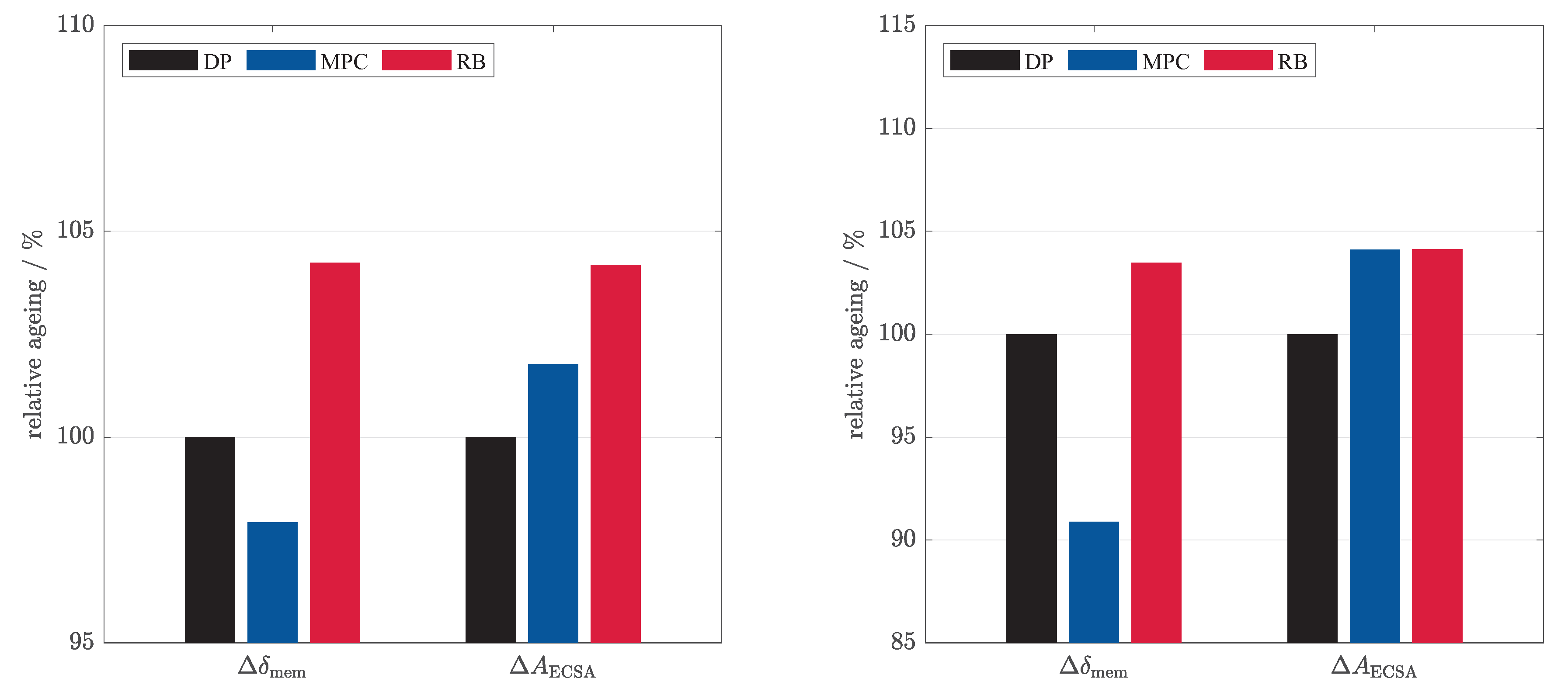
The fuel cell degradation reported in this section is calculated by an ECSA-aging model integrated into the stack model described in sec:SimModel, following established literature on electrochemically active surface area (ECSA) aging [57,58,59,60]. Within the MPC cost function, a cyclic-operation-induced voltage decay is represented by the state , obtained by integrating the empirically parameterized decay rate (see 15) with the dynamic-stress proxy (see 14), so that the effect of power fluctuations on the voltage loss is directly penalized during optimization. The resulting end-of-cycle degradation is evaluated through two complementary indicators based on the aging model from Thiele et al. [57]: the relative membrane thickness change () and the relative electrochemically active surface area loss (), both normalized to the DP strategy in Figure 12. While the absolute changes over a single drive cycle are small, the comparison highlights a consistent trend: the highly dynamic RB strategy leads to the largest degradation in both indicators and on both cycles, whereas the MPC attains the lowest membrane thickness loss and stays close to the globally optimal DP in terms of ECSA loss on the VECTO cycle, which is consistent with the objective of smoothing the fuel cell power trajectory.
4.1. Computing Time Analysis
In order to evaluate how the length of the prediction horizon H affects the computation time and the optimality of the results, a variation of the horizon lengths is performed and analyzed. Previously, the change in execution time was investigated by varying the maximum iteration steps, with the result that the optimum solution was achieved within the defined maximum SQP iteration steps in each computation step, so this consideration is ignored. For this purpose, a cycle similar to the VECTO long haul is evaluated within the MiL for a horizon range of 50–1000 s. The considered execution time is the total execution time of the S-function of the OCP in Simulink per sample time1. The maximum computation value occurring within the entire cycle is used as the reference value for the analysis, as this value is more meaningful in terms of execution on an ECU. The choice of prediction horizon has a direct influence on the execution time of the MPC. As the horizon increases, the optimum performance trajectory for each grid point is calculated for that period into the future. To quantify this influence, the cycle was run with the horizon lengths:
Figure 8 shows the progression of the target variables as a function of the horizon length of the MPC. It can be seen that the maximum execution time increases as the horizon length increases. The maximum execution time at 500 s and 600 s falls out of the pattern and is less than the execution time at 400 s. From a horizon length of 800 s, the maximum permissible execution time of 300 ms is exceeded. If executed on a controller, the MPC would run into task overruns, which must be avoided. Since the average execution time increases only slightly with increasing horizon length, but the cell voltage loss decreases significantly with increasing horizon length. At horizon length below 200 s the gradient of the cell voltage loss is significantly higher, thus with regards to the cell voltage loss a horizon length from at least 200 s should be chosen. It can be seen that a horizon length of 400 s reflects a good compromise between the lowest possible maximum execution time, low fuel consumption, low deviation from the target SoC and cell voltage loss. As a result of this parameter analysis, a prediction horizon of 400 s is selected for further investigation.
4.2. MPC vs. DP
4.2.1. VECTO Long Haul Cycle
In the following, the model predictive control approach is compared to a DP with respect to its optimality. The DP is designed to compute an optimal SoC trajectory, taking into account the minimum fuel consumption and the rate of change of fuel cell system power. The same boundary conditions and performance constraints are applied to both the MPC and the DP in order to compare the results. Due to the deviation of the mathematical system model in the MPC and DP from the simulation model in the MiL environment, a balanced state of charge at the end of the driving cycle cannot be guaranteed. In order to be able to guarantee the comparability of the consumption results nevertheless, the charge deviations in fuel consumption must be taken into account. A correction is therefore applied in both directions, so that all strategies are evaluated at an identical, balanced charge level at the end of the cycle. In the case of a positive charge deviation (), the energy missing in the battery is converted into an additional fuel mass to be applied, taking into account the overall efficiency, so that no artificial fuel consumption advantage is created. Conversely, in the case of a negative charge deviation (), which can occur, for example, due to extended recuperation during downhill driving, the surplus energy remaining in the battery is credited as an equivalent fuel mass and deducted from the consumption. Both cases are covered by the same correction rule formulated in [61] according to equation
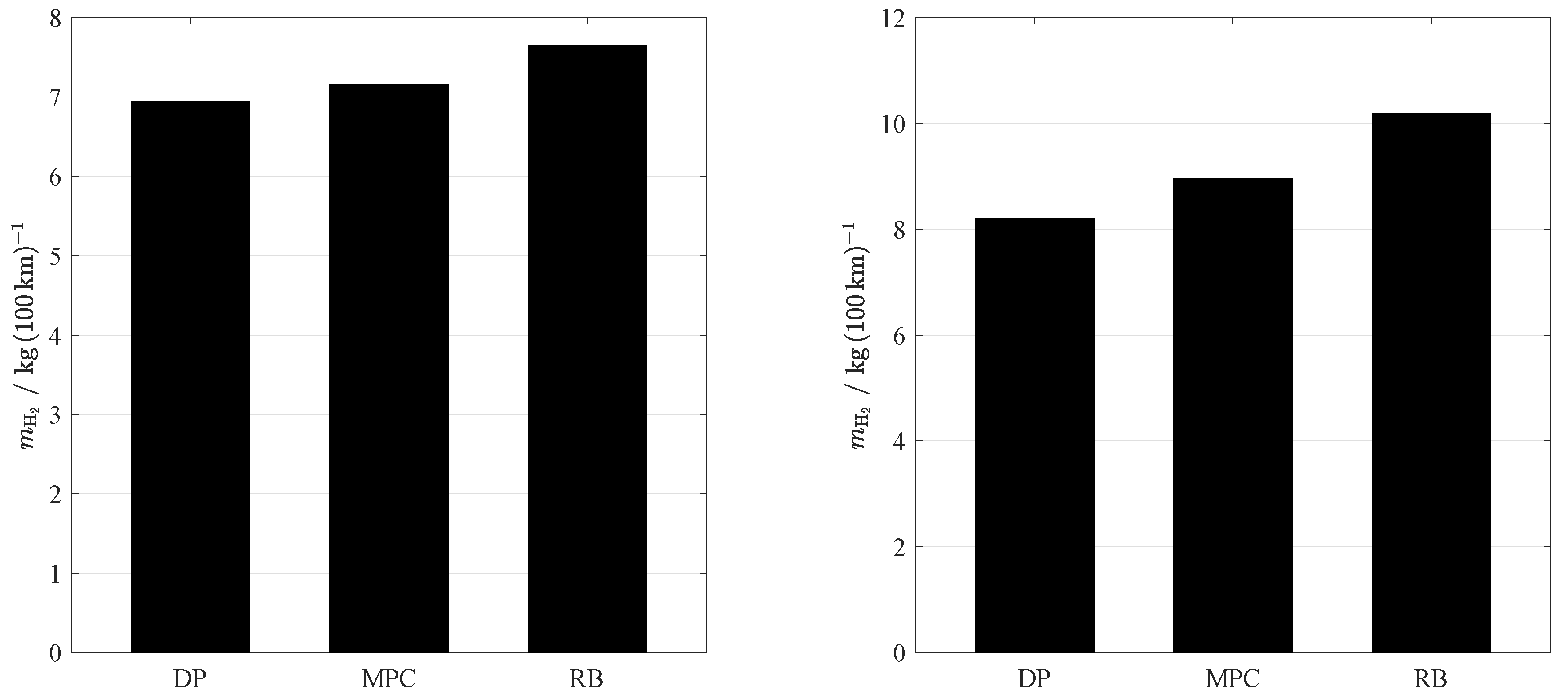
which adjusts the fuel mass determined from the simulation as a function of the charge difference. For the fuel cell system efficiency an average efficiency from the drive cycle is used. The overall efficiency is the efficiency of the electrical path and includes the fuel cell, the inverter and the battery. The results of the corrected hydrogen consumption between the DP, MPC and RB strategy of the two drive cycles can be seen in Figure 11 and Figure 11.
The fuel cell system power and state of charge (SoC) trajectories of DP and MPC in the MiL environment using the gradient and speed profile for the VECTO Long Haul cycle are compared in Figure 9. The DP controller maintains a nearly constant fuel cell power of about 95 kW, which is close to one-third of the fuel cell’s maximum power and therefore in the range of the best efficiency point for fuel cell system operation. The power trajectory of the MPC, on the other hand, is considerably more dynamic and varies between a minimum of about 25 kW and a maximum of about 217 kW. These differences in power trajectories also affect the SoC trajectories. The DP allows a wider range of SoC to be covered compared to the MPC, due to its knowledge of the entire driving profile.
Within the prediction horizon , the MPC searches for the optimal fuel cell power from which the SoC trajectory is derived. It tries to achieve the target SoC at the end of the horizon which is reflected in the maximum deviation of the SoC within the prediction horizon. The SoC of the DP reaches its minimum at and drops to a value of about 41 %. The DP thus uses 34 % of the allowed SoC operating range (i.e., the permissible SoC band between and ). The SoC of the MPC reaches its minimum of 51 % at and its global maximum of 66.8 % at , thus using 26 % of the allowed SoC range. From the results obtained, a SoC deviation from the desired target SoC can be determined for both the MPC and the DP. The MPC misses the target SoC by and has a state of charge of 59.4 % at the end of the cycle, while the DP ends at a state of charge of 60.6 %, i.e. 0.93 % above the target SoC. After correcting the fuel consumption for the state of charge deviation at the end of the cycle, the fuel consumption for the MPC is 7.18 kg. With a fuel consumption of 6.97 kg, the globally optimal DP control therefore consumes 2.9 % less hydrogen than the MPC control.
4.2.2. Aachen-Eifel Real Driving Cycle
Figure 10 shows a comparison between the FC system power trajectories and the SoC trajectories of DP and MPC in a MiL environment using the gradient and speed profile of the Aachen-Eifel real driving cycle over time. The main difference between global and local optimal control is evident in the SoC power trajectories. The DP control, which benefits from global information about the driving profile, mostly performs in the range of optimal efficiency and minimum fuel consumption, similar to the VECTO Long Haul cycle. However, the DP control mostly operates in a narrow band between about 55 kW and 65 kW, with isolated peaks up to 95 kW due to the influence of the gradient and speed profile.
Unlike the MPC, the DP detects the high-speed section at the end of the cycle and charges the battery more initially, reaching a maximum SoC of 75.4 % at before drawing it down to a minimum of 29.1 % at . As a result, the DP regulates a more constant fuel cell power output throughout the cycle to maintain low hydrogen consumption and high efficiency. On the other hand, the MPC reaches a global maximum SoC of 73.1 % at . Due to its limited knowledge of the driving cycle information according to the defined finite time horizon, the power output of the MPC differs from the power output of the DP, resulting in a more dynamic trajectory and a maximum power of 244 kW at . The DP uses a substantially larger part of the allowed SoC range (77 %) compared to the MPC (43 %). The final SoC of the DP control is 59.9 %, which is 0.2 % below the target SoC and the final SoC of the MPC control is 63.6 %, which is 6.1 % above the target SoC. With respect to the total hydrogen consumption, the advantage of the global optimality of the DP is clearly visible. After correcting the charge deviation for the MPC and DP control to the target SoC, the total hydrogen consumption of the MPC is 7.65 kg, which is 10.7 % higher than the DP’s consumption of 6.91 kg. Although the MPC does not reach the global optimum of the DP, it provides the power split in real time. In the next step the MPC is compared to a rule-based strategy.
4.3. MPC vs. Rule-Based Strategy
4.3.1. VECTO Long Haul Cycle
In this section, the MPC is compared to a rule-based (RB) strategy with respect to fuel consumption and end-of-cycle fuel cell stack degradation for the VECTO Long Haul drive cycle. The RB strategy corrects the fuel cell power demand based on the deviation of actual and reference SoC, taking into account the minimum and maximum defined fuel cell power limitations. The results of the desired fuel cell power and the SoC trajectory can be seen in Figure 9. Due to the penalization of the SoC deviation in the RB strategy, the power trajectory of the fuel cell is very dynamic with high power peak demands to minimize the deviation at all times. The power output varies between a minimum of about 25 kW and a maximum of 254.6 kW at . This can also be seen in the trajectory of the SoC with a global minimum SoC of 54.7 % at and a maximum SoC of 66.3 % due to recuperation at about . Due to the non-predictive characteristic of the RB strategy and the braking process at the end of the cycle, a final SoC above the target SoC of 60 % is achieved. The final SoC of the RB strategy is 63.9 %, which is 6.4 % above the target SoC. After correcting the fuel consumption for the state of charge deviation at the end of the cycle, the total hydrogen consumption of the RB strategy is 7.67 kg, which is 6.9 % higher than the MPC’s consumption of 7.18 kg.
The end-of-cycle fuel cell degradation is evaluated via the relative membrane thickness change () and the relative electrochemically active surface area loss (), based on the aging model from Thiele et al. [57] and normalized to the DP strategy in Figure 12. For the VECTO cycle, the dynamic RB strategy exhibits the highest degradation, with a membrane thickness loss 4.2 % and an ECSA loss 4.2 % above the DP level. The MPC, by contrast, remains close to the globally optimal DP, with a membrane thickness loss 2.1 % below and an ECSA loss only 1.8 % above the DP level, reflecting its smoother fuel cell power trajectory. The corresponding comparison for the RDE cycle is shown in Figure 12.
4.3.2. Aachen-Eifel Real Driving Cycle
In this section, the MPC is compared to a rule-based (RB) strategy with respect to fuel consumption and end-of-cycle fuel cell stack degradation for the Aachen-Eifel real driving cycle. The results of the desired fuel cell power and the SoC trajectory can be seen in Figure 10. Due to the more dynamic elevation and velocity profile, this is also reflected in the power output of the RB strategy with more fuel cell power peaks to minimize the SoC deviation at all times. This can also be seen in the trajectory of the SoC with a maximum charge deviation down to an SoC of 48.6 %. The SoC reaches a maximum value of about 74.4 % at . The final SoC of the RB strategy is 68.1 %, which is 13.5 % above the target SoC. After correcting the charge deviation for the RB strategy to the target SoC, the total hydrogen consumption is 8.75 kg, which is 14.3 % higher than the MPC’s consumption of 7.65 kg. The same trend is observed for the Aachen-Eifel real driving cycle in Figure 12. The RB strategy again shows the highest degradation, with a membrane thickness loss 3.5 % and an ECSA loss 4.1 % above the DP level. The MPC attains the lowest membrane thickness loss of all three strategies, 9.1 % below the DP level, but reaches an ECSA loss of 4.1 % above the DP level. Owing to its smoother power trajectory, the MPC therefore avoids the additional membrane degradation caused by the highly dynamic operation of the RB strategy, whereas in terms of ECSA loss the MPC and the RB strategy are practically on the same level on this cycle.
As shown in Figure 12, the DP achieves the lowest ECSA loss of the three strategies, whereas the MPC exhibits the lowest membrane thickness loss. This can be explained by the fact that the DP predominantly operates at a highly efficient, low-current operating point and therefore at a comparatively high cell voltage, whereas the MPC, due to its limited prediction horizon, more frequently commands higher load points, i.e., lower cell voltages, in order to reach the target SoC at the end of each horizon. Since the formation rate of hydrogen peroxide and the resulting chemical, voltage-dependent membrane degradation (e.g., via the associated fluoride release rate) is known to increase with cell voltage [62], higher operating voltages tend to accelerate membrane degradation. This voltage-dependent chemical degradation pathway is not implemented in the fuel cell model used within the hybrid energy management system, in order to limit modeling complexity (see [63] for a broader discussion of prescriptive lifetime management approaches for PEM fuel cell systems). This explains why the DP, despite its higher operating efficiency, does not also achieve the lowest membrane thickness loss. It should be noted that, as a first step, the aging models used in this work have only been checked for plausibility and have not yet been validated against real measurement data.
To assess the transferability of these findings to a different driving profile, all three hybrid strategies were additionally evaluated on the more dynamic Aachen-Eifel real driving cycle (cf. ). The qualitative trends observed for the VECTO Long Haul cycle are confirmed: the DP and the MPC end the cycle close to the target SoC, whereas the non-predictive RB strategy overshoots it by 13.5 %, and the ranking of the aging indicators follows the same pattern as for the VECTO cycle. However, the results also reveal that the advantage of the DP over the MPC becomes more pronounced under the more dynamic load profile of the Aachen-Eifel cycle, whereas the MPC achieves a closer approximation of the DP’s global optimum on the comparatively steadier VECTO Long Haul cycle.
Figure 11.
Comparison of the corrected hydrogen consumption between the DP, MPC and RB strategy for the (fig:CompHydConsumption) VECTO Long Haul cycle and the (fig:CompHydConsumptionRural) Aachen-Eifel real driving (rural road) cycle.
Figure 11.
Comparison of the corrected hydrogen consumption between the DP, MPC and RB strategy for the (fig:CompHydConsumption) VECTO Long Haul cycle and the (fig:CompHydConsumptionRural) Aachen-Eifel real driving (rural road) cycle.
Regarding applicability to a degraded stack, the methodology remains applicable as long as the MPC prediction model is updated to the actual stack condition. In practice, this can be achieved by (i) initializing the degradation-related state (and/or SoH) to the current value and (ii) updating the polarization-curve-based voltage model (and, if necessary, the efficiency/BoP maps) to reflect the degraded performance. The OCP structure, constraints, and real-time implementation remain unchanged; only the model parameters and initial conditions need to be adapted.
Figure 12.
Comparison of the relative membrane thickness () and the relative electrochemically active surface area () at the end of the cycle between the DP, MPC and RB strategy for the (fig:CompAging) VECTO Long Haul cycle and the (fig:CompAgingRural) Aachen-Eifel real driving (rural road) cycle.
Figure 12.
Comparison of the relative membrane thickness () and the relative electrochemically active surface area () at the end of the cycle between the DP, MPC and RB strategy for the (fig:CompAging) VECTO Long Haul cycle and the (fig:CompAgingRural) Aachen-Eifel real driving (rural road) cycle.
5. Conclusions
In this work, a model predictive control approach was developed for the calculation of an optimal fuel cell power trajectory for a heavy duty fuel cell truck. To compute the power trajectory, the optimization problem was formulated using the open source software package acados in MATLAB Simulink. Based on the cost function defined in this work, the optimal control trajectory is computed and transferred to the system model as a target fuel cell power curve. By taking into account the power gradient in the cost function, the MPC was able to achieve constant operation in terms of avoiding large power fluctuations, which has a positive effect on the lifetime of the fuel cell system. A good trade-off between computational time and optimality was found based on a parameter analysis of important target variables of the MPC to evaluate the influence of the length of the prediction horizon.
The developed optimization algorithm was successfully implemented in an existing model-in-the-loop environment and the functionality of the optimization algorithm was validated and tested using different driving cycles. In addition, a comparison of the developed MPC with a global optimal DP was performed with respect to hydrogen consumption and with a RB strategy with respect to aging of the fuel cell. The result of the comparison shows for typical truck driving profiles for the VECTO Long Haul a consumption advantage of the DP over the MPC of 2.9 %. For a more dynamic cycle that does not have a typical heavy duty truck driving profile, the MPC approach consumed 10.7 % more hydrogen than the DP for the Aachen-Eifel real driving cycle. The SoH of the fuel cell was derived by calculating the cell voltage drop based on the standard deviation of five consecutive fuel cell outputs over time as well as via the membrane thickness reduction. However, since the SoH depends on a large number of factors, the cell voltage loss calculated in this work based on empirically determined values was used for a simplified representation of the SoH. Due to the limited information about the fuel cell dynamics from the polarization curve, the simplified SoH is only intended to illustrate the degradation effects of power variations and does not represent the magnitude of various other effects. Within this work, the MPC reduced the end-of-cycle fuel cell degradation relative to the rule-based strategy. On the VECTO Long Haul cycle, the membrane thickness loss and the ECSA loss of the MPC were 6.1 % and 2.3 % lower than those of the RB strategy. On the dynamic RDE cycle the membrane thickness loss of the MPC was 12.2 % lower, whereas the ECSA loss of both strategies was practically identical.
With respect to different powertrain designs, the proposed control strategy is flexible because the OCP formulation is based on generic power and energy balances, component maps, and constraints. A change in component sizing (e.g., stack rated power, battery capacity, DC/DC limits, or auxiliary sizing) primarily affects the steady-state maps (fuel cell efficiency, BoP power) and the admissible operating region (power and SoC constraints), while the MPC structure and real-time implementation remain unchanged. This also makes the approach suitable as a control layer in co-optimization environments: additional objectives (e.g., thermal limits, operating cost, or mission-level constraints) and updated component models can be integrated by extending the stage cost and constraints without changing the underlying solver workflow. Finally, the general MPC/OCP framework is not restricted to heavy-duty road transport and can be adapted to other application domains (e.g., aviation) by replacing the vehicle/mission model, updating constraints and safety requirements, and using domain-specific fuel cell system models.
In the simulation environment, the specified cycle is assumed to be a real driving scenario in which the truck follows the speed profile. In real driving scenarios, this profile cannot be followed exactly due to various environmental influences. To capture the real driving situation within the MPC, telemetry data of the traffic and a predictive model, e.g. in the form of a Markov chain model, would be required to predict the new driving profile information and make it available to the MPC. By adding telemetry and a predictive model, MPC control could be used as a real-time application in real driving scenarios. In addition, the SoC trajectory generated by the DP could be used as a reference SoC for MPC control.
Author Contributions
Conceptualization, S.M., A.W. and S.P.; methodology, S.M.; software, S.M. and A.W.; validation, S.M., A.W. and S.P.; formal analysis, S.M.; investigation, S.M.; resources, V.S. and J.S.; data curation, S.M.; writing—original draft preparation, S.M.; writing—review and editing, S.M., A.W., V.S., J.S., A.E. and S.P.; visualization, S.M.; supervision, S.P. and A.E.; project administration, S.P.; funding acquisition, S.P. All authors have read and agreed to the published version of the manuscript.
Funding
The presented work has been done as part of the research project “ReforceHIL” (03EN5004A-C) that is supported within the 7th Energy Research Program: Innovations for Energy Transition by the Federal Ministry for Economic Affairs and Climate Action. The APC was funded by RWTH Aachen University.
Institutional Review Board Statement
Not applicable.
Informed Consent Statement
Not applicable.
Data Availability Statement
Data are contained within the article.
Conflicts of Interest
The authors declare no conflicts of interest. The funders had no role in the design of the study; in the collection, analyses or interpretation of data; in the writing of the manuscript; or in the decision to publish the results.
Acknowledgments
The authors gratefully acknowledge the support of the ReforceHIL project partners.
Abbreviations
The following abbreviations are used in this manuscript:
| A-ECMS | Adaptive Equivalent Consumption Minimization Strategy |
| BoL | Beginning of Life |
| BoP | Balance of Plant |
| CU | Control Unit |
| DP | Dynamic Programming |
| ECMS | Equivalent Consumption Minimization Strategy |
| EF | Equivalence Factor |
| EM | Electrical Machine |
| EMS | Energy Management Strategy |
| EoL | End of Life |
| ESS | Energy Storage System |
| EV | Electric Vehicle |
| FCEV | Fuel Cell Electric Vehicle |
| FL | Fuzzy Logic |
| GDL | Gas Diffusion Layer |
| HCU | Hybrid Control Unit |
| HDV | Heavy-Duty Vehicle |
| HV | High-Voltage |
| KKT | Karush-Kuhn-Tucker |
| LB | Learning-Based |
| MEA | Membrane Electrode Assembly |
| MiL | Model-in-the-Loop |
| MPC | Model Predictive Control |
| MPL | Micro-Porous Layer |
| NOP | Nonlinear Optimization Problem |
| OB | Optimization-Based |
| OCP | Optimal Control Problem |
| OCV | Open Circuit Voltage |
| PEMFC | Proton Exchange Membrane Fuel Cell |
| PMP | Pontryagin’s Minimum Principle |
| RB | Rule-Based |
| RCP | Rapid Control Prototyping |
| RHC | Receding Horizon Control |
| RL | Reinforcement Learning |
| SC | Supercapacitor |
| SDP | Stochastic Dynamic Programming |
| SoC | State of Charge |
| SoH | State of Health |
| SQP | Sequential Quadratic Programming |
| VECTO | Vehicle Energy Consumption Calculation Tool |
References
- The Paris Agreement, 2015.
- Reducing carbon emissions: EU targets and policies, 2018.
- Colnago, S.; Mauri, M.; Piegari, L. Energy Management Strategy for a Fuel cell/Lead acid battery/ Ultracapacitor hybrid electric vehicle. [CrossRef]
- Silvas, E.; Hofman, T.; Murgovski, N.; Etman, P.; Steinbuch, M. Review of Optimization Strategies for System-Level Design in Hybrid Electric Vehicles. 2016. [Google Scholar] [CrossRef]
- Abad, A.V.; Dodds, P.E. Green hydrogen characterisation initiatives: Definitions, standards, guarantees of origin, and challenges. Energy Policy 2020, 138, 111300. [Google Scholar] [CrossRef]
- Tran, D.D.; Vafaeipour, M.; El Baghdadi, M.; Barrero, R.; van Mierlo, J.; Hegazy, O. Thorough state-of-the-art analysis of electric and hybrid vehicle powertrains: Topologies and integrated energy management strategies. [CrossRef]
- Yu, P.; Li, M.; Wang, Y.; Chen, Z. Fuel Cell Hybrid Electric Vehicles: A Review of Topologies and Energy Management Strategies. 2022. [Google Scholar] [CrossRef]
- Emran, A.; Garg, S.; Mertes, S.; Gautam, A.; Schmidt, M.; Wick, M.; Walters, M.; Wagh, S.; Sharma, V. Fuel Cell Electric Metro Train Concept – Zero Emission Rail Transport Solution for Indian Cities. 2024. [Google Scholar] [CrossRef]
- Jia, H.; Tang, J.; Yu, Y.; Sun, Y.; Yin, B.; Zhang, C. Energy Management Strategy of Fuel Cell/Battery Hybrid Vehicle Based on Series Fuzzy Control. Int. J. Automot. Technol. 2021, 22, 1545–1556. [Google Scholar] [CrossRef]
- Biswas, A.; Emadi, A. Energy Management Systems for Electrified Powertrains: State-of-the-Art Review and Future Trends. IEEE Trans. Veh. Technol. 2019, 68, 6453–6467. [Google Scholar] [CrossRef]
- Azib, T.; Bethoux, O.; Remy, G.; Marchand, C.; Berthelot, E. An Innovative Control Strategy of a Single Converter for Hybrid Fuel Cell/Supercapacitor Power Source. IEEE Trans. Ind. Electron. 2010, 57, 4024–4031. [Google Scholar] [CrossRef]
- Fu, Z.; Li, Z.; Si, P.; Tao, F. A hierarchical energy management strategy for fuel cell/battery/supercapacitor hybrid electric vehicles. Int. J. Hydrogen Energy 2019, 44, 22146–22159. [Google Scholar] [CrossRef]
- Geng, B.; Mills, J. K.; Sun, D. Two-Stage Energy Management Control of Fuel Cell Plug-In Hybrid Electric Vehicles Considering Fuel Cell Longevity. IEEE Trans. Veh. Technol. 2012, 61, 498–508. [Google Scholar] [CrossRef]
- Murphey, Yi L.; Chen, ZhiHang; Kiliaris, Leonidas; Masrur, M. Abul. Intelligent power management in a vehicular system with multiple power sources. J. Power Sources 2011, 196, 835–846. [Google Scholar] [CrossRef]
- Li, W.; Ye, J.; Cui, Y.; Kim, N.; Cha, S.W.; Zheng, C. A Speedy Reinforcement Learning-Based Energy Management Strategy for Fuel Cell Hybrid Vehicles Considering Fuel Cell System Lifetime. Int. J. Precis. Eng. Manuf.-Green Technol. 2022, 9, 859–872. [Google Scholar] [CrossRef]
- Zhu, Y.; LI, X.; Liu, Q.; Li, S.; Xu, Y. Review article: A comprehensive review of energy management strategies for hybrid electric vehicles. Mech. Sci. 2022, 13, 147–188. [Google Scholar] [CrossRef]
- Yang, S.; Ghate, A.; Zhu, Q.; Prucka, R. An interpretable reinforcement learning approach for emission and fuel optimization in heavy-duty hybrid electric vehicles. Energy Convers. Manag. 2025, 120459. [Google Scholar] [CrossRef]
- Salay, R.; Queiroz, R.; Czarnecki, K. An Analysis of ISO 26262: Using Machine Learning Safely in Automotive Software. arXiv 2017, arXiv:1709.02435. [Google Scholar] [CrossRef]
- Liu, X.; Srivastava, V.; Pan, W.; Schaub, J.; Sun, J.; Tian, X.; Deng, Y.; Xiong, J.; Wu, X.; Muthyala, P.; et al. Real-time Multi-Layer Predictive Energy Management for a Plug-in Hybrid Vehicle based on Horizon and Navigation Data. In Proceedings of the WCX SAE World Congress Experience. SAE International, 2024. https://doi.org/10.4271/2024-01-2773. 2024. [CrossRef]
- Z. Chen.; N. Guo.; Q. Zhang.; J. Shen.; R. Xiao. An Optimized Rule Based Energy Management Strategy for a Fuel Cell/Battery Vehicle. In Proceedings of the 2017 IEEE Vehicle Power and Propulsion Conference (VPPC), 2017, pp. 1–6. https://doi.org/10.1109/VPPC.2017.8330991. 2017. [CrossRef]
- Zhou, Y.; Ravey, A.; Péra, M.C. Real-time cost-minimization power-allocating strategy via model predictive control for fuel cell hybrid electric vehicles. Energy Convers. Manag. 2021, 229, 113721. [Google Scholar] [CrossRef]
- Ferrara, Alessandro; Hametner, Christoph; Jakubek, Stefan. Health-conscious predictive energy management strategy for fuel cell electric trucks. Energy Rep. 2024, 12, 5961–5973. [Google Scholar] [CrossRef]
- Ferrara, Alessandro; Jakubek, Stefan; Hametner, Christoph. Cost-optimal design and energy management of fuel cell electric trucks. Int. J. Hydrogen Energy 2023, 48, 16420–16434. [Google Scholar] [CrossRef]
- Hemi, H.; Ghouili, J.; Cheriti, A. Combination of Markov chain and optimal control solved by Pontryagin’s Minimum Principle for a fuel cell/supercapacitor vehicle. Energy Convers. Manag. 2015, 91, 387–393. [Google Scholar] [CrossRef]
- J. Bernard.; S. Delprat.; F. Buechi.; T. M. Guerra. Global Optimisation in the power management of a Fuel Cell Hybrid Vehicle (FCHV). In Proceedings of the 2006 IEEE Vehicle Power and Propulsion Conference, 2006, pp. 1–6. https://doi.org/10.1109/VPPC.2006.364289. 2006. [CrossRef]
- Song, K.; Wang, X.; Li, F.; Sorrentino, M.; Zheng, B. Pontryagin’s minimum principle-based real-time energy management strategy for fuel cell hybrid electric vehicle considering both fuel economy and power source durability. Energy 2020, 205, 118064. [Google Scholar] [CrossRef]
- Huangfu, Y.; Li, P.; Pang, S.; Tian, C.; Quan, S.; Zhang, Y.; Wei, J. An Improved Energy Management Strategy for Fuel Cell Hybrid Vehicles Based on Pontryagin’s Minimum Principle. IEEE Trans. Ind. Appl. 2022, 58, 4086–4097. [Google Scholar] [CrossRef]
- Aubeck, F. Modulary structured optimization of the energy management in hybrid vehicles. Dissertation, Rheinisch-Westfälischen Technischen Hochschule Aachen, Aachen, 2022.
- Zhang, Y.; Chen, M.; Cai, S.; Hou, S.; Yin, H.; Gao, J. An online energy management strategy for fuel cell hybrid vehicles. In Proceedings of the 2021 40th Chinese Control Conference (CCC), 2021; pp. 6034–6039. [Google Scholar] [CrossRef]
- Muthyala, P.; Mayank, M.; Ünver, B.; Han, S.E.; Uzunoğlu, B.; Kaydeci, A.B.; Toğuş, F.; Schaub, J.; Virnich, L.; Pischinger, S. Comparative study of real-time A-ECMS and rule-based energy management strategies in long haul heavy-duty PHEVs. Energy Convers. Manag. X 2024, 23, 100679. [Google Scholar] [CrossRef]
- Arce, Alicia; del Real, Alejandro J.; Bordons, Carlos. MPC for battery/fuel cell hybrid vehicles including fuel cell dynamics and battery performance improvement. J. Process Control 2009, 19, 1289–1304. [Google Scholar] [CrossRef]
- Li, Tianyu; Liu, Huiying; Ding, Daolin. Predictive energy management of fuel cell supercapacitor hybrid construction equipment. Energy 2018, 149, 718–729. [Google Scholar] [CrossRef]
- Desantes, J.M.; Novella, R.; Lopez-Juarez, M.; Nidaguila, I. Experimental assessment of a heavy-duty fuel cell system in relevant operating conditions. Appl. Energy 2024, 376, 124293. [Google Scholar] [CrossRef]
- Aliberti, P.; Minneci, M.; Sorrentino, M.; Cuomo, F.; Musto, C. Efficiency-Based Modeling of Aeronautical Proton Exchange Membrane Fuel Cell Systems for Integrated Simulation Framework Applications. Energies 2025, 18, 999. [Google Scholar] [CrossRef]
- Aliberti, P.; Simone, C.; Addesso, P.; Piano, G.D.; Dons`i, F.; Galdi, A.; Maritato, L.; Pantani, R.; Pianese, C.; Polverino, P.; et al. Fuel cells in aviation: challenges to power the future of flight. Energy Convers. Manag. X 2026, 29, 101426. [Google Scholar] [CrossRef]
- Xu, N.; Kong, Y.; Chu, L.; Ju, H.; Yang, Z.; Xu, Z.; Xu, Z. Towards a Smarter Energy Management System for Hybrid Vehicles: A Comprehensive Review of Control Strategies. Appl. Sci. 2019, 9. [Google Scholar] [CrossRef]
- Frey, J.; Baumgärtner, K.; Frison, G.; Diehl, M. Multi-Phase Optimal Control Problems for Efficient Nonlinear Model Predictive Control with acados, 2024, [arXiv:math.OC/2408.07382]. arXiv:math.
- Robin Verschueren.; Gianluca Frison.; Dimitris Kouzoupis.; Jonathan Frey.; Niels van Duijkeren.; Andrea Zanelli.; Branimir Novoselnik.; Thivaharan Albin.; Rien Quirynen.; Moritz Diehl. acados – a modular open-source framework for fast embedded optimal control <bold>2021</bold>. https://doi.org/10.1007/s12532-021-00208-8.
- Srivastava, V.; Wendler, A.; Schaub, J.; Walters, M.; Thodupunoori, S.; Mulukutla, K. Modular Fuel Cell Control Software for Commercial Vehicle Applications. 2024. [Google Scholar] [CrossRef]
- Emran, A.; Mertes, S.; Garg, S.; Wick, M.; Walters, M.; Sharma, V. Fuel Cell Electric Vehicles - An Optimal Solution for Future Electrification of Heavy Commercial Vehicles in India. In Proceedings of the 2021 IEEE Transportation Electrification Conference (ITEC-India). IEEE, 2021, pp. 1–8. https://doi.org/10.1109/ITEC-India53713.2021.9932475. [CrossRef]
- Sallach, D.; Weber, N.; Cäsar, J.; Hinrichs, N.; Ennen, A.; Mertes, S.; Pischinger, S.; Kampker, A.; Vallery, H.; Jeschke, P. HyInnoPEM <bold>2025</bold>.
- Liu, Y.; Dirkes, S.; Kohrn, M.; Wick, M.; Pischinger, S. A high-fidelity real-time capable dynamic discretized model of proton exchange membrane fuel cells for the development of control strategies. J. Power Sources 2022, 537. [Google Scholar] [CrossRef]
- Dickinson, E.J.F.; Smith, G. Modelling the Proton-Conductive Membrane in Practical Polymer Electrolyte Membrane Fuel Cell (PEMFC) Simulation: A Review. Membranes 2020, 10. [Google Scholar] [CrossRef] [PubMed]
- Satterfield, M.B.; Benziger, J.B. Non-Fickian water vapor sorption dynamics by Nafion membranes. J. Phys. Chem. B 2008, 112 12, 3693–3704. [Google Scholar] [CrossRef] [PubMed]
- Colpan, Can O.; Nalbant, Yagmur; Ercelik, Mustafa. 4.28 Fundamentals of Fuel Cell Technologies. In Comprehensive Energy Systems; Dincer, Ibrahim, Ed.; Elsevier: Oxford, 2018; pp. 1107–1130. [Google Scholar] [CrossRef]
- Dirk Abel, A.B. Rapid Control Prototyping: Methoden und Anwendungen; Springer Berlin Heidelberg: Berlin, Heidelberg, 2006. [Google Scholar] [CrossRef]
- Coralli, A.; Sarruf, B.J.; de Miranda, P.E.V.; Osmieri, L.; Specchia, S.; Minh, N.Q. Fuel Cells. [CrossRef]
- Lin, Xinyou; Xu, Xinhao; Lin, Haibo. Predictive-ECMS based degradation protective control strategy for a fuel cell hybrid electric vehicle considering uphill condition. eTransportation 2022, 12, 100168. [Google Scholar] [CrossRef]
- Stevens, Matthew. Hybrid Fuel Cell Vehicle Powertrain Development Considering Power Source Degradation. 2009. [Google Scholar] [PubMed]
- Jouin, M.; Bressel, M.; Morando, S.; Gouriveau, R.; Hissel, D.; Péra, M.C.; Zerhouni, N.; Jemei, S.; Hilairet, M.; Bouamama, B.O. Estimating the end-of-life of PEM fuel cells: Guidelines and metrics. Appl. Energy 2016, 177, 87–97. [Google Scholar] [CrossRef]
- Lin, Chan-Chiao; Peng, Huei; Grizzle, J.W.; Kang, Jun-Mo. Power management strategy for a parallel hybrid electric truck. IEEE Trans. Control Syst. Technol. 2003, 11, 839–849. [Google Scholar] [CrossRef]
- Lenz, Martin; Hoehl, Tobias; Mertes, Simon; Pischinger, Stefan. Applying a numerical optimization to determine the entropic heat coefficient of a battery. Appl. Therm. Eng. 2022, 211, 118467. [Google Scholar] [CrossRef]
- Lenz, Martin; Mertes, Simon; Beecks, Paul-Julius; Viertel, Pascal; Pischinger, Stefan. Generating characteristic maps of battery cell parameters from sparse input data. J. Power Sources 2021, 503, 230054. [Google Scholar] [CrossRef]
- Hsieh, Y.M.; Liu, Y.C. Model predictive control strategy for plug-in hybrid electric vehicles. In Proceedings of the 2016 14th International Conference on Control, Automation, Robotics and Vision (ICARCV), 2016; pp. 1–6. [Google Scholar] [CrossRef]
- Papageōrgiu, M.; Leibold, M.; Buss, M. Optimierung: Statische, dynamische, stochastische Verfahren für die Anwendung, 4. In Lehrbuch, korrigierte auflage ed.; Springer Vieweg: Berlin and Heidelberg, 2015. [Google Scholar]
- Vehicle Energy Consumption calculation TOol - VECTO, 2017.
- Thiele, P.; Gouveia, L.; Ulrich, O.; Yang, Y.; Liu, Y.; Wick, M.; Pischinger, S. Realistic accelerated stress tests for PEM fuel cells: Operation condition dependent load profile optimization. J. Power Sources 2024, 617, 234959. [Google Scholar] [CrossRef]
- Jahnke, T.; Futter, G.A.; Baricci, A.; Rabissi, C.; Casalegno, A. Physical Modeling of Catalyst Degradation in Low Temperature Fuel Cells: Platinum Oxidation, Dissolution, Particle Growth and Platinum Band Formation. J. Electrochem. Soc. 2020, 167, 013523. [Google Scholar] [CrossRef]
- You, H.; Fu, J.; Li, X. Research on ECSA Degradation Model for PEM Fuel Cell under Vehicle Conditions. In Proceedings of the 2020 4th CAA International Conference on Vehicular Control and Intelligence (CVCI), 2020. [Google Scholar] [CrossRef]
- Ma, Y.; Zhang, J.; Yang, K.; Lin, Q.; Sun, B.; Hu, Z.; Zhai, S. Data-driven electrochemically active surface area loss modeling and its application in fuel cell stack degradation prediction. J. Power Sources 2025, 659, 238354. [Google Scholar] [CrossRef]
- Aubeck, F.; Lenz, M.; Mertes, S.; Zylka, K.; Pischinger, S. Generic stochastic particle filter algorithm for predictive energy optimization of a Plug-in Hybrid Electric Vehicle extended by a battery temperature control and implemented on a Hardware-in-the-Loop system. Control Eng. Pract. 2022, 120. [Google Scholar] [CrossRef]
- Dirkes, S.; Leidig, J.; Fisch, P.; Pischinger, S. Prescriptive Lifetime Management for PEM Fuel Cell Systems in Transportation Applications, Part II: On-board Operando Feature Extraction, Condition Assessment and Lifetime Prediction. Energy Convers. Manag. 2023, 283, 116943. [Google Scholar] [CrossRef]
- Dirkes, S.; Leidig, J.; Fisch, P.; Pischinger, S. Prescriptive Lifetime Management for PEM Fuel Cell Systems in Transportation Applications, Part I: State of the Art and Conceptual Design. Energy Convers. Manag. 2023, 277, 116598. [Google Scholar] [CrossRef]
| 1 | Windows 10 desktop PC with an Intel Xeon W-2123 at a clock speed of 3.6 GHz and 64 GB RAM |
Figure 1.
General comparison of studied EMSs [4].
Figure 1.
General comparison of studied EMSs [4].
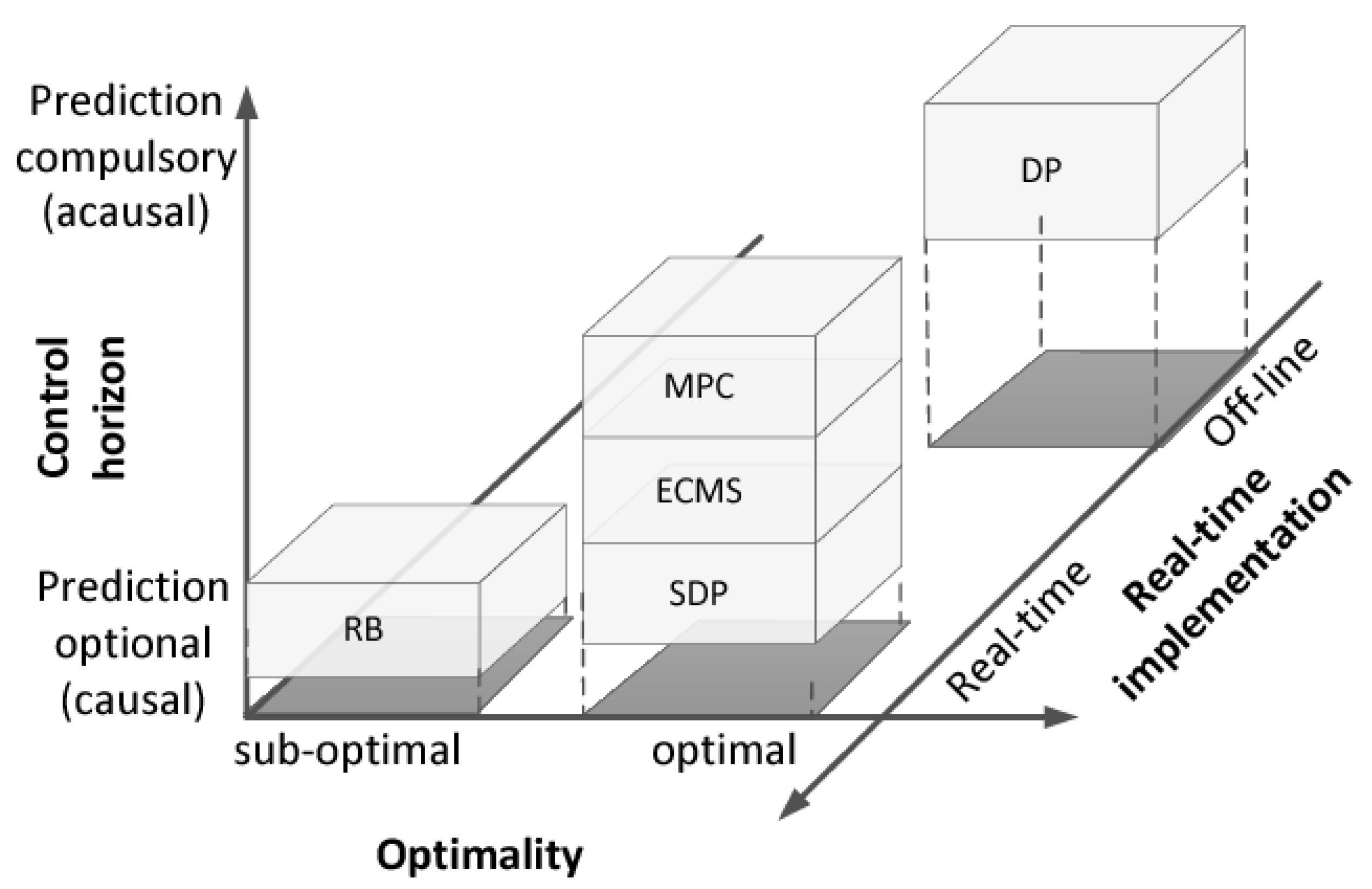
Figure 2.
Comparison of the various operating strategies for FCEVs in terms of optimality, computing effort, real-time capability, computing time and implementation effort (according to [36]).
Figure 2.
Comparison of the various operating strategies for FCEVs in terms of optimality, computing effort, real-time capability, computing time and implementation effort (according to [36]).
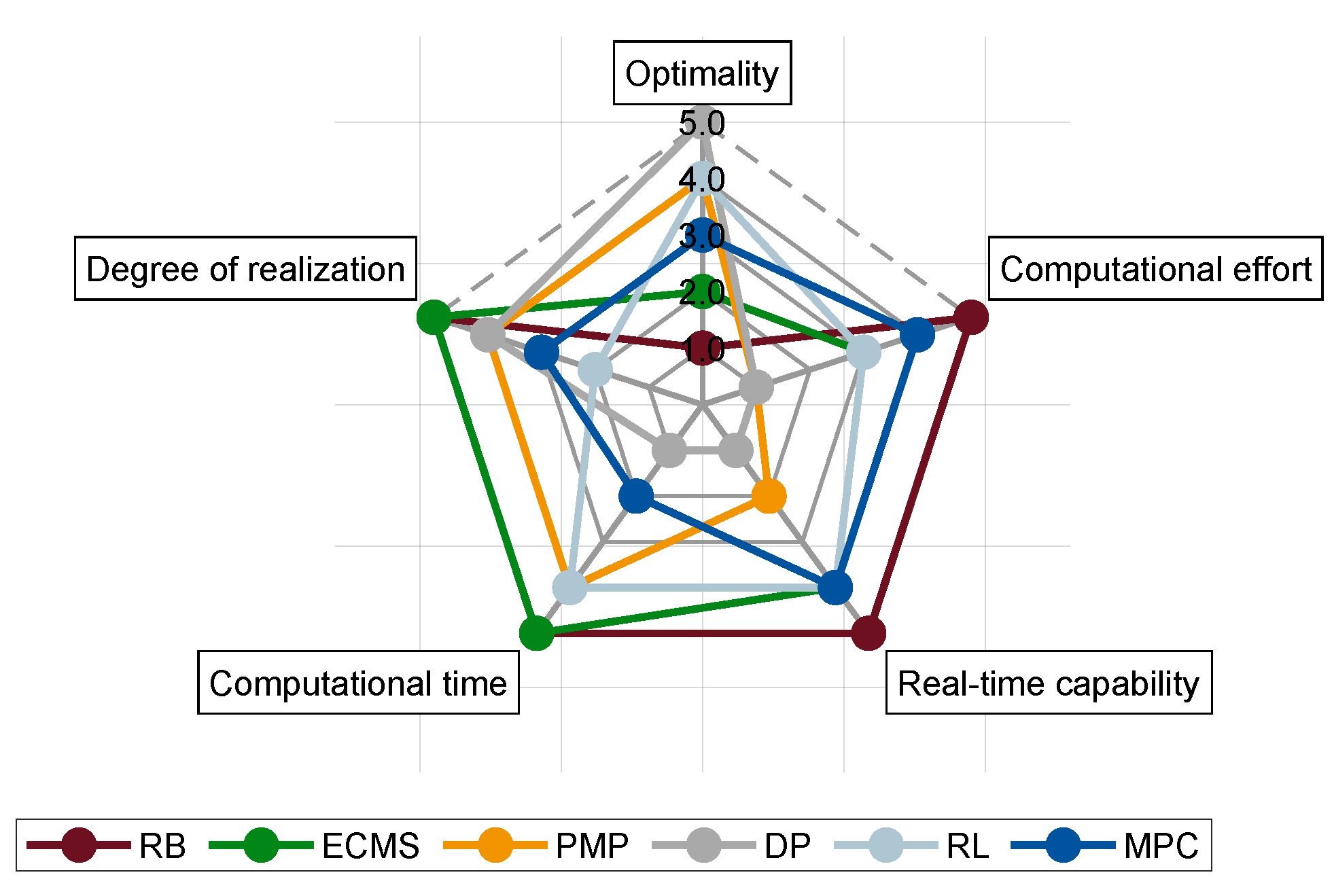
Figure 3.
Segmentation of the cell in the in-plane and the through-plane direction.
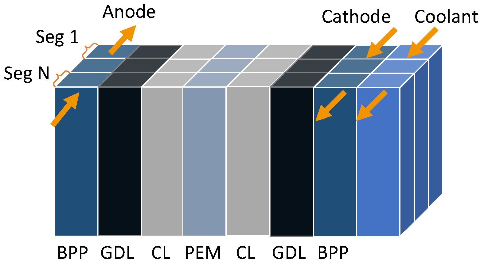
Figure 4.
Optimal Control Problem (OCP) for minimization of hydrogen consumption and degradation of fuel cell.
Figure 4.
Optimal Control Problem (OCP) for minimization of hydrogen consumption and degradation of fuel cell.
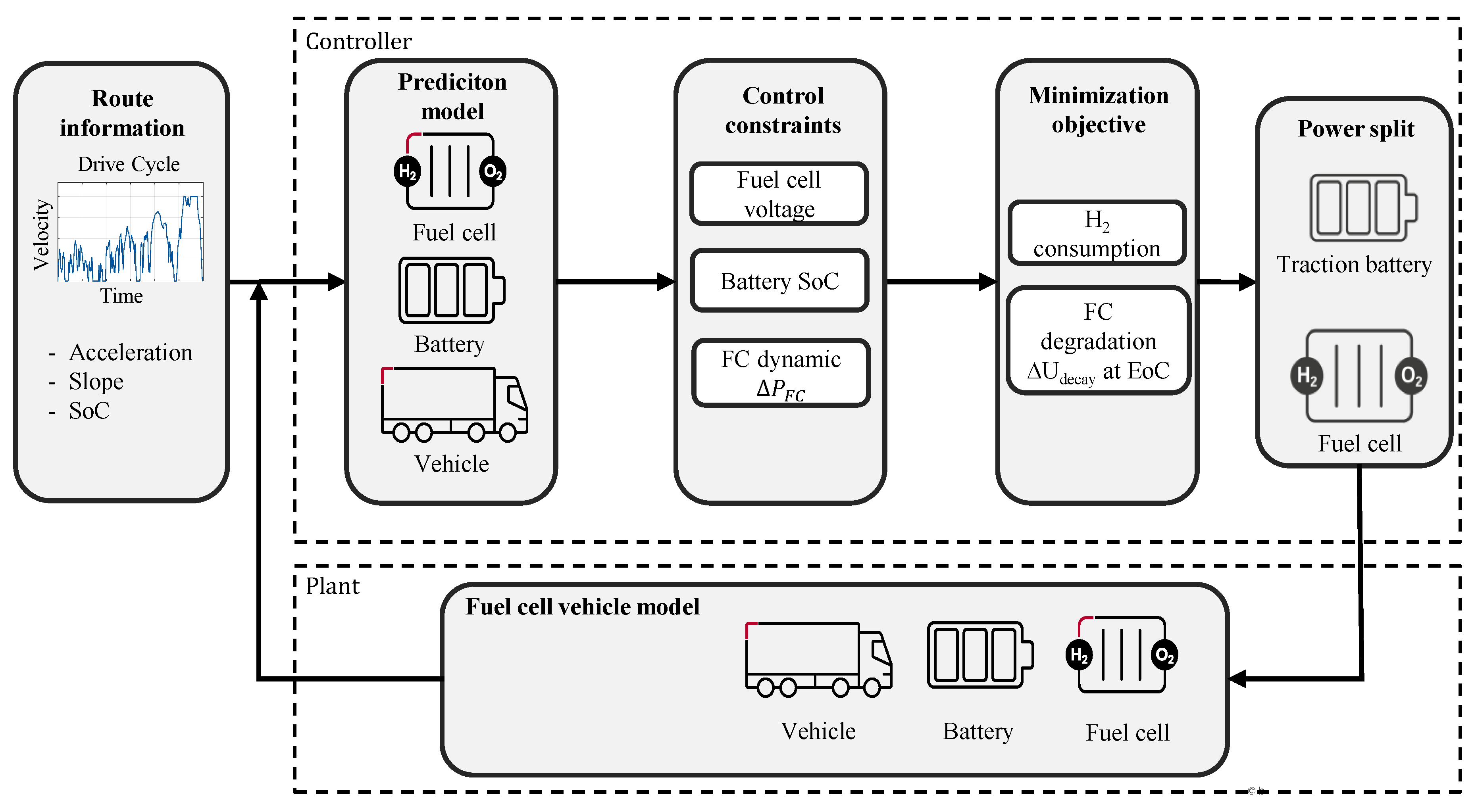
Figure 5.
Electrical equivalent circuit diagram of the traction battery.
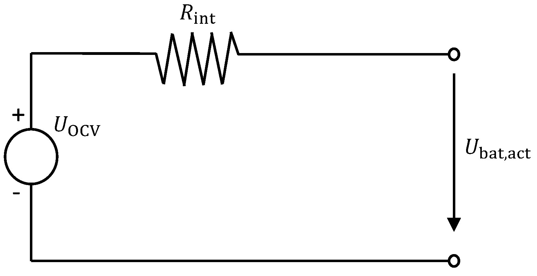
Figure 6.
VECTO Long Haul drive cycle velocity and slope profile.
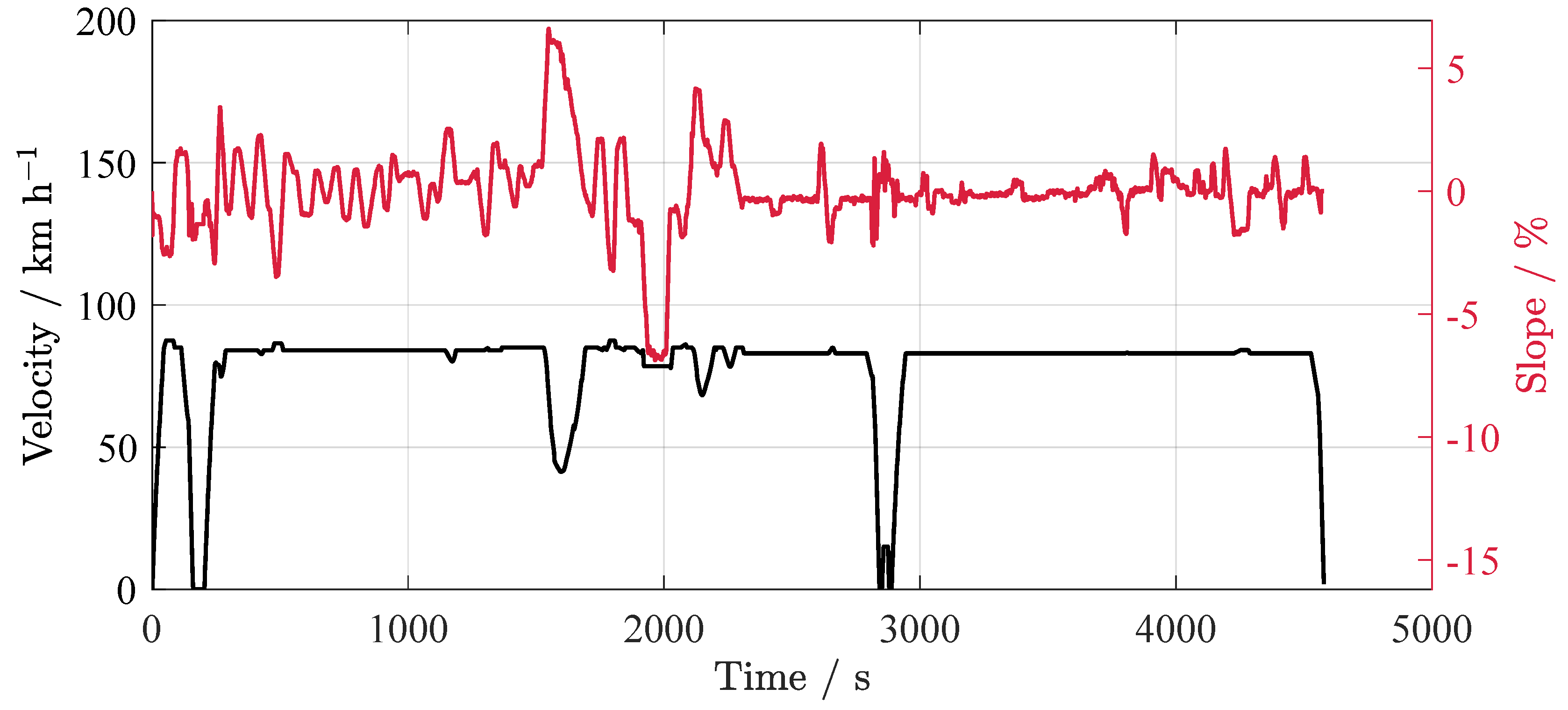
Figure 7.
Aachen-Eifel real driving cycle velocity and slope profile.
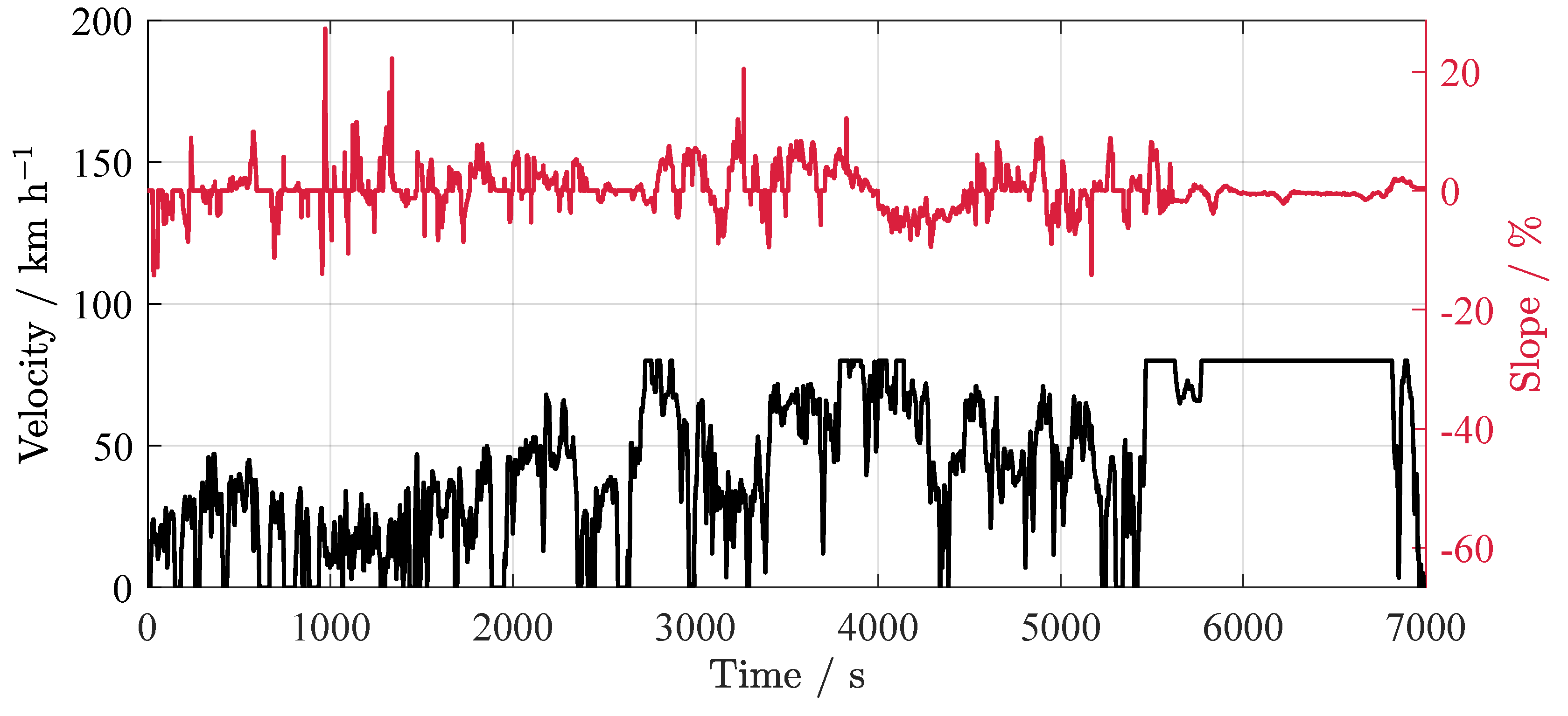
Figure 8.
Effect of varying the prediction horizon length H on the deviation from the target SoC, fuel consumption, cell voltage loss and the maximum execution time of the MPC.
Figure 8.
Effect of varying the prediction horizon length H on the deviation from the target SoC, fuel consumption, cell voltage loss and the maximum execution time of the MPC.
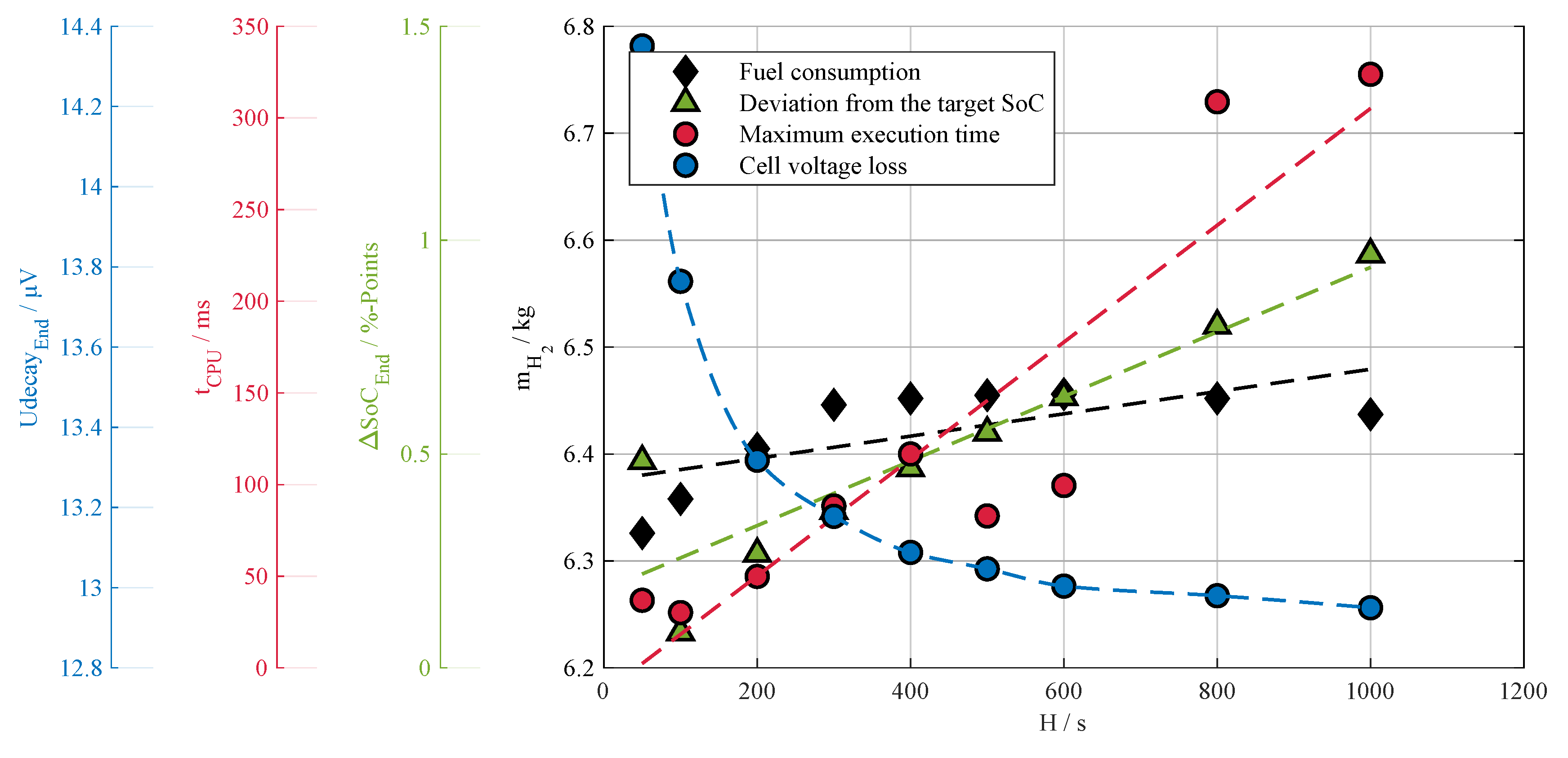
Figure 9.
Comparison of the FC system power trajectory and the SoC trajectories between the DP, MPC and RB control (prediction horizon 400 s) in the MiL environment with gradient and speed profile of the VECTO Long Haul cycle. While the DP tries to maintain the target SoC only at the end of the cycle, the MPC tries to achieve the target SoC at the end of each horizon.
Figure 9.
Comparison of the FC system power trajectory and the SoC trajectories between the DP, MPC and RB control (prediction horizon 400 s) in the MiL environment with gradient and speed profile of the VECTO Long Haul cycle. While the DP tries to maintain the target SoC only at the end of the cycle, the MPC tries to achieve the target SoC at the end of each horizon.
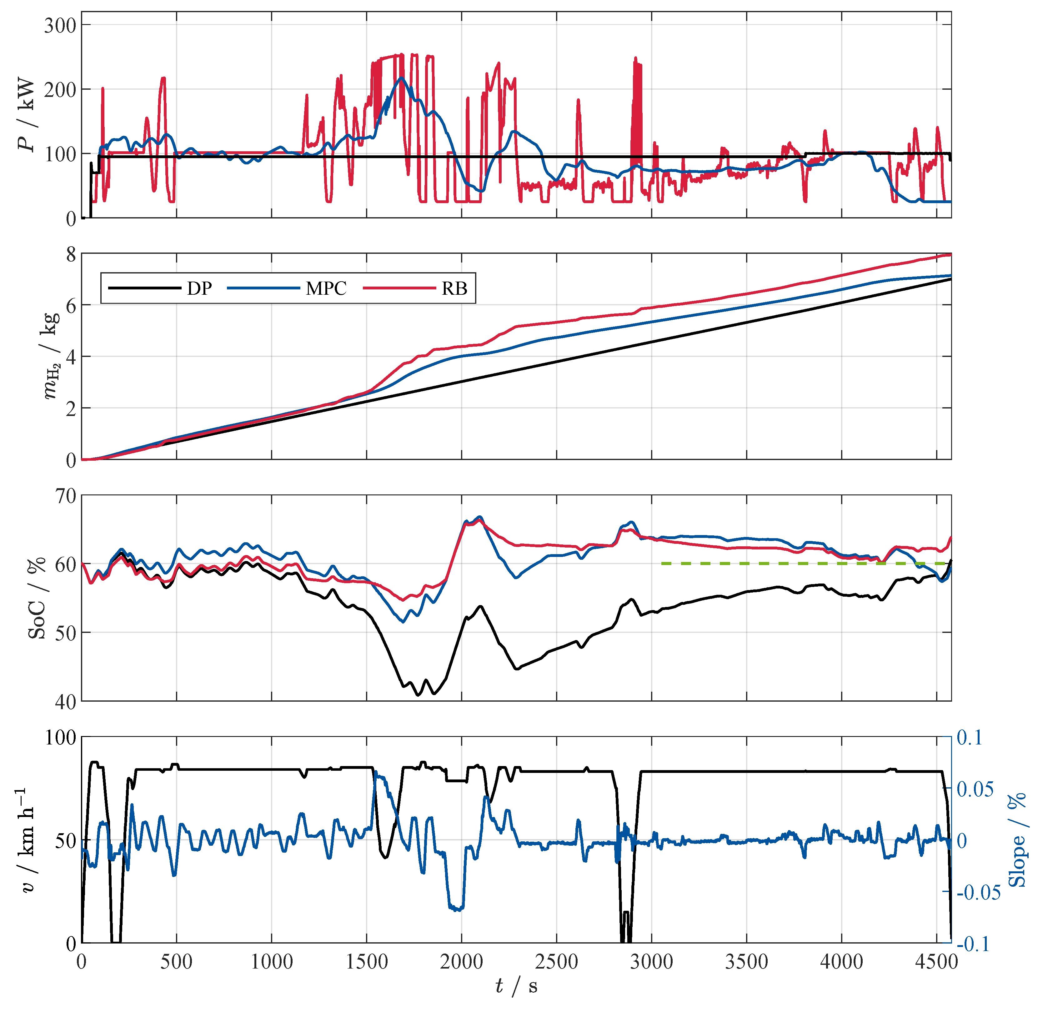
Figure 10.
Comparison of the FC system power trajectory and the SoC trajectories between the DP, MPC and RB control in the MiL environment with gradient and speed profile of the Aachen-Eifel real driving cycle. The green dashed line indicates the target SoC of 60 %.
Figure 10.
Comparison of the FC system power trajectory and the SoC trajectories between the DP, MPC and RB control in the MiL environment with gradient and speed profile of the Aachen-Eifel real driving cycle. The green dashed line indicates the target SoC of 60 %.
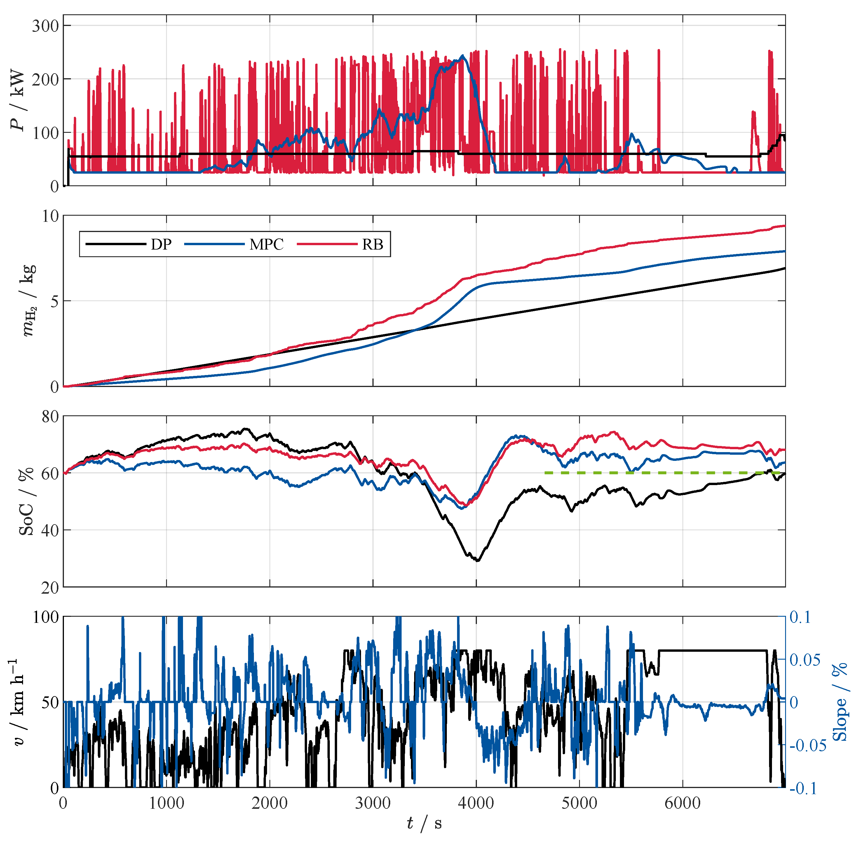

Table 1.
Vehicle specification.
| Parameter | Symbol | Unit | Value |
|---|---|---|---|
| Vehicle weight | t | 30 | |
| Tire specification | — | — | 295/80 R22.5 |
| Front surface | m2 | 9.7 | |
| Drag coefficient | — | 0.53 | |
| Rolling coefficient | — | 0.00467 | |
| Max. velocity | km/h | 90 |
Table 2.
EDU specification.
| Parameter | Symbol | Unit | Value |
|---|---|---|---|
| EDU peak power | kW | 500 | |
| Max. motor speed | rpm | 3400 | |
| Battery capacity | kWh | 98.84 | |
| Fuel cell peak power | kW | 303.6 |
Disclaimer/Publisher’s Note: The statements, opinions and data contained in all publications are solely those of the individual author(s) and contributor(s) and not of MDPI and/or the editor(s). MDPI and/or the editor(s) disclaim responsibility for any injury to people or property resulting from any ideas, methods, instructions or products referred to in the content. |
© 2026 by the authors. Licensee MDPI, Basel, Switzerland. This article is an open access article distributed under the terms and conditions of the Creative Commons Attribution (CC BY) license (http://creativecommons.org/licenses/by/4.0/).
Copyright: This open access article is published under a Creative Commons CC BY 4.0 license, which permit the free download, distribution, and reuse, provided that the author and preprint are cited in any reuse.