
Submitted:
14 August 2026
Posted:
17 August 2026
You are already at the latest version
Abstract
Comparing heterogeneous energy pathways through a single hydrogen output can be misleading when model scale, conversion physics and evidential quality differ between pathways. This study presents a traceable numerical screening framework for photovoltaic (PV), concentrated solar power (CSP), geothermal energy and waste heat recovery (WHR) using nine PV scenarios, nine CSP scenarios, six geothermal scenarios and six WHR scenarios generated with ANSYS-based thermal or thermal-fluid models and MATLAB/Python post-processing. The PV branch provides documented DC power estimates of 33.31–65.44 W, with a mean of 51.69 W. The thermal branches are analyzed separately: their turbine workbooks contain static pressure differences and a fixed volumetric flow calculation of 1.8044 cubic metres per second for every scenario, but no documented mass flow or enthalpy coupling to the upstream heat exchanger models, rotor torque or complete expansion states. The product of static pressure difference and volumetric flow is therefore retained only as a pressure-flow power-scale diagnostic, and the subsequent efficiency scaling is reported as an illustrative electrical equivalent rather than turbine output. Within the WHR diagnostic set, excluding the deliberate high-flow stress case reduces the mean electrical equivalent from 6.635 to 4.245 kW, showing a 56.3% sensitivity of the arithmetic mean to that single operating point. Hydrogen estimates for PV and hydrogen equivalents for the thermal diagnostics are reported in separate evidential classes and are not compared as technology performance. The numerical dataset does not demonstrate common capacity/resource normalization, grid independence, quantitative validation or a closed energy balance from thermal resource to turbine. The contribution is therefore methodological: a transparent screening architecture that preserves the physical meaning, scale, coupling status and evidence level of each quantity before any downstream interpretation.
Keywords:
hydrogen production
; photovoltaic
; concentrated solar power
; geothermal energy
; waste heat recovery
; computational fluid dynamics
; electrolysis
; energy conversion
; numerical screening
; numerical traceability
1. Introduction
Hydrogen produced by electrolysis can connect variable or otherwise difficult-to-use energy resources with chemical storage and industrial demand. International assessments continue to identify renewable electricity and electrolyzer deployment as central elements of low-emissions hydrogen development [1,2]; system studies also emphasize the role of power-to-hydrogen when electricity supply and demand are mismatched over longer time scales [30,31]. The usefulness of hydrogen as a common end product, however, creates a methodological difficulty: identical hydrogen units can conceal very different upstream physics.
The PV pathway is fundamentally electrical. Irradiance and cell temperature modify the current-voltage response and therefore the DC power available to the downstream converter [3,4,5,17,18,19]. CSP instead concentrates solar radiation onto a receiver, so optical delivery, external heat loss and internal convection determine the thermal state available to a power cycle [6,7,20,21,22,23]. Geothermal conversion depends on the temperature and flow of the produced fluid, heat exchanger performance and the selected cycle, with scaling, corrosion and pumping becoming relevant when a simplified model is transferred to a real brine system [8,9,24,25]. WHR is still more site-dependent because the recoverable temperature level, flow and allowable disturbance of the host process constrain the useful heat source [10,11,26,27,28,29]. These are not interchangeable boundary-value problems.
A second difficulty appears at the turbomachinery interface. A pressure difference multiplied by volumetric flow has dimensions of power and is appropriate in specific hydraulic/head formulations, but a static pressure loss measured across a simplified CFD geometry is not automatically recoverable shaft work. Turbine work is normally established from rotor torque and angular velocity or from a thermodynamic change in stagnation enthalpy across a controlled expansion [12]. Conflating dissipative pressure loss with useful work can reverse the interpretation of a design comparison: a larger loss may indicate a greater penalty rather than a better turbine.
This study analyzes a four-pathway numerical dataset around this distinction. The objective is not to create a universal ranking of PV, CSP, geothermal energy and WHR, but to determine which comparisons remain defensible when the upstream models differ in physical meaning, prototype scale and verification status. The framework uses three rules: quantities are reported only when they are documented in the available simulation or post-processing data; derived quantities are recalculated only from documented source variables and assumptions; and unavailable numerical details are identified explicitly rather than reconstructed from typical CFD practice.
The resulting contribution is a traceable numerical screening framework with an explicit evidence hierarchy. It preserves the operating-point values generated by the pathway models, reclassifies the thermal pathway pressure-flow calculation as a comparative diagnostic, isolates the WHR high-flow stress case and separates numerical consistency from validation. Because the upstream thermal models and downstream turbine spreadsheets do not share a documented mass flow or thermodynamic state interface, the thermal downstream mapping is treated as a separate diagnostic rather than as a closed heat-to-shaft energy balance. This structure supports screening while identifying the additional evidence required before design-scale or technology-ranking claims are made.
2. Materials and Methods
2.1. Comparative Scope and Evidence Basis
Figure 1 summarizes the screening architecture. PV and the heat-driven pathways share scenario management and post-processing conventions but not the same upstream physics. The PV branch maps cell thermal states to the available DC power estimate. CSP, geothermal and WHR provide thermal-fluid fields and pressure/flow outputs, while the separate turbine stage spreadsheets provide a pressure-flow diagnostic. No documented mass flow or enthalpy state transfer links the thermal resource models quantitatively to that turbine stage calculation; the downstream thermal mapping is therefore not interpreted as a closed energy-conversion chain.
The numerical evidence is divided into three levels. Level 1 comprises direct exports and documented input parameters from the available spreadsheets, CSV files and launcher scripts. Level 2 comprises quantities recalculated algebraically from Level 1 values using explicitly documented assumptions. Level 3 covers information that cannot be recovered from the available project material, including grid refinement data and several Fluent solver settings. Level 3 quantities are not inferred from engineering defaults.

Table 1.
Evidence hierarchy applied to the numerical screening framework.
| Level | Content | Treatment in this paper |
|---|---|---|
| 1 | Scenario inputs; PV cell-average temperatures and final DC outputs; CSP heat transfer export; geothermal/WHR inlet/outlet states; static pressures; mass flow/density values; documented post-processing constants. | Reported directly, with units and scenario provenance. |
| 2 | , , the efficiency-scaled electrical equivalent indicator, hydrogen equivalent mass and stoichiometric water minimum. | Recalculated from Level 1 values; interpretation is explicitly limited. |
| 3 | Mesh counts/quality, turbulence closure, wall treatment, detailed Fluent numerics, grid convergence, quantitative experimental validation, complete turbine thermodynamic states and common capacity/resource normalization. | Not reconstructed; treated as missing verification/reproducibility information. |
Table 2.
Energy chain closure status. The table distinguishes physically connected calculations from separate diagnostic mappings.
Table 2.
Energy chain closure status. The table distinguishes physically connected calculations from separate diagnostic mappings.
| Interface | Status | Interpretation in this paper |
|---|---|---|
| PV thermal state → PV DC estimate | Partially documented | Final DC values are available, but the exact final temperature correction equation is not recoverable. |
| CSP imposed receiver flux → reported heat transfer | Documented within the reduced-order CSP model | Used as a thermal response only; no optical ray tracing is claimed. |
| Geothermal/WHR source conditions → outlet thermal states | Documented as operating-point states | Temperature responses are analyzed; archived direct heat transfer rate fields are zero and are not reinterpreted. |
| Thermal models → turbine diagnostic | Not closed | The turbine workbooks use a fixed that is not derived from the upstream heat exchanger mass flow or enthalpy state. |
| Pressure-flow diagnostic → electrical equivalent | Algebraic mapping only | is an illustrative electrical equivalent, not resolved shaft or generator power. |
| Electrical quantity → hydrogen metric | Algebraic mapping only | PV yields an energy-based hydrogen estimate; thermal branches yield hydrogen equivalents that inherit the diagnostic limitations above. |
2.2. Numerical Workflow and Documented CFD Configuration
The available launch scripts call the ANSYS Workbench executable identified as v241. The project material documents ANSYS thermal/thermal-fluid calculations, MATLAB-based scenario launching and MATLAB/Python post-processing. Several boundary parameters can be recovered, but a complete Fluent setup cannot. Table 3 separates documented information from unresolved solver details.
Several turbine stage workbook rows contain generic fields corresponding to a 1 s time increment, a 10 s flow time field and 100 iterations. Because the associated Fluent journal, formulation and residual histories are unavailable, these fields are not treated as evidence of a particular transient scheme or of converged final iteration counts.
The absence of grid refinement evidence is material. Current CFD verification practice separates iterative convergence from discretization error assessment; grid convergence or an equivalent discretization study is required before quantitative claims of mesh independence are made [15,16,32,33]. The results below are therefore reported as prototype-scale numerical operating points, not validated design predictions.
A separate Supplementary Information document accompanies this manuscript and provides a verification evidence status table together with the processed scenario datasets and derivation notes used in the analysis. The available project material does not contain the cell/element counts and mesh quality statistics, a coarse/medium/fine refinement sequence, Grid Convergence Index (GCI) values, residual histories, mass or energy imbalance histories, or an experimental validation dataset. These quantities are therefore identified explicitly as unavailable rather than replaced by assumed values.
2.3. Scenario Definitions
2.4. PV Thermal–Electrical Post-Processing
The PV workbook contains 32 cell-average temperatures for each scenario, 32 corrected cell voltages, a series voltage, a series current and a final DC power value. The PV launcher table fixes surface emissivity at 0.85 and uses the scenario-specific irradiance/heat flux, ambient temperature and convection coefficient inputs reported in Table 4. It also contains a fixed field labelled “Heat Flow” with value 0.1, but the available files do not document its physical application sufficiently for interpretation. The final workbook states that the results were corrected using a “32-cell temperature coefficient model” and were not produced by the preliminary Shockley-diode fit in the MATLAB development script. The exact final temperature coefficient equation and its reference parameters are unavailable, so the electrical model is not reconstructed from the preliminary script.
The reported PV electrical quantity is the final documented DC estimate,
with , and taken from the final workbook. This preserves the numerical results while avoiding a false claim of reproducibility for the missing correction law. Temperature dependence of PV output is well established in standard performance models, where irradiance and cell temperature modify the current–voltage characteristic [3,4,5,17,18,19].
2.5. CSP Reduced-Order Receiver Representation
The CSP model does not resolve the optical field by ray tracing. Instead, a receiver heat flux is prescribed as a reduced-order representation of the optical stage. This is consistent with a thermal receiver study but cannot quantify intercept factor, tracking error, mirror slope error or nonuniform concentration from first principles. Detailed trough-receiver models show that optical delivery, receiver heat loss and internal convection are separate components of the collector problem [6,7,20,21,22,23].
The fixed CSP fluid, tube and thermal properties are summarized in Table 6. The parameter file documents a fluid inlet velocity of 0.5 m , emissivity of 0.85 and a receiver temperature condition of 150 °C. Both tube_thickness and tube_thickness_geometry are 0.002 m for all nine scenarios; this value is therefore used as the documented geometry input. A separate legacy export field P92 is also labelled tube thickness and contains 0.010 m. Because its physical meaning is undefined, it is treated as ambiguous export metadata rather than as a second geometry specification. The reported CSP heat transfer output, , is used directly rather than reconstructed.
2.6. Geothermal and WHR Thermal Resource Models
The geothermal branch is an operating-point heat recovery model, not a closed geothermal plant. Hot-side temperature and velocity, cold-side velocity and outlet temperatures are available. The direct “total heat transfer rate” field in the geothermal workbook is zero for all scenarios and is therefore not treated as a physical heat transfer result. A complete geothermal power model would additionally require a specified working fluid/cycle, pumping demand, brine chemistry and site constraints. Binary ORC systems are commonly used to exploit medium- and low-temperature geothermal resources, but cycle optimization requires thermodynamic states that are absent from the available dataset [8,24,25]. Corrosion and scaling are likewise material heat exchanger constraints in real geothermal fluids and are outside the present model [9].
The WHR branch uses hot gas temperature and velocity, cold-side conditions and outlet states. As with the geothermal workbook, the WHR “total heat transfer rate” field is zero and is not reinterpreted. WHR feasibility is inseparable from the host process: useful recovery must be compatible with the available heat source and with pressure and back pressure constraints imposed by the host process [10,11,26,27,28,29]. WHR-S5 doubles the baseline hot source velocity from 3 to 6 m and increases the documented hot source mass flow value from 185.4 to 370.8 kg ; it is treated as a stress/sensitivity point rather than a representative annual operating condition.
2.7. Energy Chain Closure and Pressure-Flow Diagnostic
The separate turbine stage workbooks calculate a static pressure difference and volumetric flow rate as
In all three turbine stage workbooks, the volumetric flow calculation uses kg and kg , giving the same for every scenario. The workbooks explicitly use this mass flow field because another available flow field was flagged as producing a nonphysical duct velocity. This fixed is not derived from the upstream CSP, geothermal or WHR heat exchanger mass flow. Consequently, the upstream thermal resource models and this turbine stage calculation are not quantitatively coupled by a documented mass flow or thermodynamic state interface, and scenario-to-scenario variation in the pressure-flow diagnostic is driven by the static pressure difference rather than by an independently resolved turbine flow rate.
The CSP and geothermal post-processing assumption sheets also store a 0.18 m turbine diameter, a 0.20 m duct diameter, 24 blades and a tip-speed-ratio value of 1.5. Those values were used to generate algebraic RPM and torque estimates. The torque column is calculated from the assumed shaft power scale divided by an estimated angular velocity; it is not torque extracted from a rotating CFD domain. These geometry and kinematic assumptions are therefore documented but are not used as evidence of resolved turbomachinery performance.
The available pressure and flow values do not establish that the pressure change is a controlled expansion through an energy-extracting rotor. To prevent a dissipative loss from being misidentified as useful work, this study defines
which is termed the pressure-flow power-scale indicator. Its unit is watt, but its evidential meaning is limited to the product of the documented static pressure difference and the fixed workbook volumetric flow. A larger value is not, by itself, evidence of higher turbine efficiency or shaft power.
The turbine stage post-processing documents and . Those factors are used only to reproduce an illustrative electrical equivalent mapping:
Equation (4) is a diagnostic mapping, not a validated generator output and not an energy balance closed to the upstream thermal resource model. A resolved turbine would normally require direct mechanical power,
or, for a thermodynamic turboexpander under appropriate assumptions, a thermodynamic work relation based on mass flow and the change in stagnation enthalpy, for example
with efficiencies and losses defined consistently [12]. The available files contain neither resolved rotor torque from CFD nor the complete thermodynamic state set needed for Equation (6). The fixed 48 V DC bus in the post-processing is therefore kept only as a prototype reference for converting an electrical equivalent quantity to current; it is not proposed as an industrial bus voltage for systems operating from the kilowatt (kW) to megawatt (MW) scale.
2.8. Electrolyzer and Water Indicators
The downstream electrolyzer is an energy balance block rather than an electrochemical stack model. PEM electrolysis performance depends on stack voltage, load, operating pressure, temperature and balance-of-plant demand [13,14,30]. The specific electricity assumption used in the post-processing is
A value of this order is compatible with stack-level PEM electricity requirements reported in authoritative technical targets, while a complete system can require additional balance-of-plant energy [13,14]. For PV, the hydrogen estimate is calculated from ; for the thermal pathways, the same mapping is applied to and is therefore labelled a hydrogen equivalent indicator:
with consistent conversion between kW and kWh. The value is treated as an engineering assumption rather than fitted to a particular electrolyzer. The stoichiometric reaction gives a theoretical minimum water mass of approximately
This quantity is the stoichiometric minimum and excludes purification, cooling, purges and other plant water uses [34]. No polarization curve, pressure dependence, dynamic response or degradation model is included [14].
2.9. Scale Compatibility, Normalization and Uncertainty Status
No common installed capacity, collector/module area, resource energy input or exergy denominator is documented consistently across all four pathways. The mean PV DC estimate is 0.05169 kW, whereas the thermal diagnostic electrical equivalents are 3.287 kW for CSP, 3.964 kW for geothermal energy and 4.245 kW for WHR when the deliberate stress case is excluded. Numerically, these thermal diagnostic values are approximately 64, 77 and 82 times the PV value, respectively. This difference primarily reflects incompatible prototype scales and different model definitions; it is not interpreted as a technology performance ratio. For this reason, the paper does not use the absolute PV and thermal values to rank the pathways, and their hydrogen metrics are reported separately by evidential class. Radar scoring and the earlier normalized heatmap across pathways are omitted because the available project material does not document a defensible weighting or common normalization basis.
The scenario ensemble provides deterministic sensitivity information but not probabilistic uncertainty quantification. Numerical verification is also incomplete because no multi-grid dataset was found. In the terminology of CFD verification and validation [15,16,32,33], the present work supports plausibility assessment and numerical consistency checks, not demonstrated grid convergence or experimental validation. This limitation is carried into the interpretation of every quantitative CFD-derived result.
3. Results
3.1. PV Operating-Point Response
The nine PV scenarios produce documented DC estimates from 33.31 to 65.44 W, with a mean of 51.69 W (Figure 2). The minimum occurs in PV-S1 at 500 W , while the maximum occurs in PV-S3 at 1000 W and 25 °C ambient temperature. At the common 800 W solar input, the cold-ambient case PV-S4 gives 56.39 W whereas the hot-desert case PV-S5 gives 48.14 W, a 14.6% reduction. The cell-average temperature rises from 31.35 ∘C in PV-S4 to 63.93 ∘C in PV-S5, consistent with the expected negative temperature dependence of maximum PV power [3,4,19].
Wind-related convection also changes the thermal operating point. At 800 W and 25 ∘C ambient, the weak-convection case ( W ) gives a cell-average temperature of 54.70 ∘C and 50.50 W, whereas the strong-convection case ( W ) gives 35.14 ∘C and 55.45 W. These values show the internal consistency of the documented thermal-to-electrical trend, although they do not substitute for validation of the final electrical correction law.
The raw PV-S3 thermal field contains a local plotted range of approximately 47.1–95.1 ∘C, whereas the 32 extracted cell-average values for the same scenario cluster around 50 ∘C. The distinction is important: a local field maximum and an area-averaged cell temperature are different observables and should not be used interchangeably in the electrical model.
3.2. CSP Heat Transfer Response
The CSP heat transfer export ranges from 2.333 to 6.421 kW. The maximum occurs in CSP-S3 under the 15,000 W imposed receiver heat flux. Figure 3 shows a positive relationship between imposed flux and the reported heat transfer result, but ambient and convection changes cause scenarios at the same imposed flux to separate. For the 10,000 W group, the heat transfer outputs span 3.702–4.805 kW. The reduced-order model with imposed flux therefore captures thermal sensitivity but cannot attribute these changes to optical concentration efficiency.
3.3. Geothermal and WHR Thermal States
At constant 0.5 m hot- and cold-side inlet velocities, increasing the geothermal source temperature from 363.15 K (GEO-S1) to 423.15 K (GEO-S3) raises the cold-outlet temperature from 340.51 to 386.37 K. At a fixed 393.15 K source temperature, increasing the hot-side velocity from 0.25 m (GEO-S4) to 1.0 m (GEO-S5) raises the cold-outlet temperature from 333.71 to 379.63 K. These operating-point trends are physically plausible for increased thermal capacity flow, but a direct geothermal heat transfer rate is not reported because the corresponding workbook field is zero.
The WHR thermal states show the same temperature-level sensitivity. At 3 m hot-side velocity, increasing the source temperature from 423.15 to 623.15 K raises the cold-outlet temperature from 349.88 to 432.38 K. The high-flow case WHR-S5 doubles the hot-side velocity to 6 m and contains a documented hot source mass flow of 370.8 kg . This scenario is deliberately separated from representative operating-point averages below because its pressure-flow product is an outlier.
Figure 4 presents selected numerical fields. Each panel has its own legend and scale and is used only to document the numerical state corresponding to the scenarios; the images are not evidence of grid independence or experimental validation.
3.4. Indicators Derived from the Pressure-Flow Diagnostic
Table 8 summarizes the thermal pathway pressure-flow quantities. CSP gives –13.85 kW and an efficiency-scaled –4.121 kW. Geothermal scenarios give –17.01 kW and –5.061 kW. WHR spans a much wider interval because WHR-S5 reaches a static pressure difference of 34.62 kPa, producing kW and kW under the documented algebraic assumptions.
Figure 5 displays each pathway-specific scenario as an independent bar rather than connecting unlike scenario indices across technologies. The plot is a diagnostic of the pressure-flow post-processing rather than a turbine performance map. In particular, the geothermal pressure-flow indicator does not vary monotonically with the geothermal heat source flow labels, and all thermal scenarios use the same workbook value of . This decoupling is another reason not to interpret as recovered thermal work.
3.5. WHR Stress-Case Sensitivity
Including WHR-S5 gives a mean of 6.635 kW. Excluding that deliberate high-flow stress case gives 4.245 kW. The mean including the stress case is 56.3% higher than the mean obtained from the remaining scenarios (Figure 6). An unqualified arithmetic mean therefore overstates the central tendency of the representative WHR scenarios. This sensitivity is reported because it exposes the dependence of the downstream indicator on the pressure-flow formulation and on source flow selection.
3.6. Hydrogen and Stoichiometric Water Mapping
The downstream mapping uses 50 kWh as an energy assumption. Because the PV and thermal branches have different scales and different evidential status, they are reported separately rather than combined into a single comparative technology table.
PV energy-based estimate.
The mean documented PV DC power of 51.69 W maps to an estimated hydrogen production of 0.0248 kg day and a stoichiometric minimum water requirement of 0.223 kg . This value belongs only to the small PV prototype represented in the workbook and is not normalized to the scale of the thermal models.
Table 9.
PV prototype downstream estimate based on the documented mean DC power.
| Basis | Mean DC power | estimate | Stoich. O minimum |
|---|---|---|---|
| (kg ) | (kg ) | ||
| PV prototype | 51.69 W | 0.0248 | 0.223 |
Thermal diagnostic hydrogen equivalents.
For CSP, geothermal and WHR, the same 50 kWh mapping is applied to . Because originates from the separate pressure-flow diagnostic rather than from a closed upstream heat-to-shaft balance, the resulting values are labelled hydrogen equivalents. They are not validated production forecasts and must not be compared directly with the PV estimate as a technology ranking.
Table 10.
Hydrogen equivalents for the thermal pathways derived from the pressure-flow diagnostic. These values are not validated hydrogen production predictions.
Table 10.
Hydrogen equivalents for the thermal pathways derived from the pressure-flow diagnostic. These values are not validated hydrogen production predictions.
| Pathway | Diagnostic basis | equivalent | Stoich. O minimum |
|---|---|---|---|
| (kg ) | (kg ) | ||
| CSP | Mean = 3.287 kW | 1.578 | 14.20 |
| Geothermal | Mean = 3.964 kW | 1.903 | 17.13 |
| WHR, all scenarios | Mean = 6.635 kW | 3.185 | 28.67 |
| WHR, S5 excluded | Mean = 4.245 kW | 2.038 | 18.34 |
The two tables intentionally separate the approximately 50 W PV prototype from kilowatt-scale thermal diagnostics. Without a common installed capacity, resource input, collector area, exergy basis or annual weighting, no quantitative superiority of one pathway over another can be inferred from these absolute values.
4. Discussion
4.1. Observed Numerical Behavior
The scenario set resolves several coherent sensitivities. PV power falls when cell temperature rises at fixed irradiance and increases when stronger convection suppresses the thermal operating point. CSP heat transfer rises with imposed receiver flux, while ambient and convection conditions shift the recovered heat at the same nominal flux. Geothermal and WHR outlet temperatures respond strongly to source temperature and source flow perturbations. These trends support physical plausibility of the scenario logic but do not establish quantitative accuracy.
The thermal pathway pressure-flow calculation behaves differently from a heat recovery metric. Its largest value occurs at WHR-S5 because the documented static pressure difference reaches 34.62 kPa while remains 1.8044 . The same is imposed by the turbine stage post-processing for every thermal scenario, so the apparent scenario variation in is mathematically proportional to the static pressure difference. The resulting outlier changes the WHR mean by more than half relative to the mean excluding the stress case. More importantly, this calculation is not quantitatively linked to the mass flow or enthalpy change on the source side from the CSP, geothermal or WHR thermal models. A larger static pressure loss may represent dissipation, a boundary condition artifact or an available head depending on where and how the pressure is defined; the available dataset does not contain the rotor or thermodynamic information required to distinguish those interpretations.
4.2. Coupling Limitation and Turbomachinery Interpretation
The central methodological limitation is the absence of a documented energy-conserving interface between the thermal resource models and the turbine stage spreadsheets. Replacing “fluid/turbine power” with a pressure-flow power-scale indicator prevents an algebraically correct unit conversion from becoming a physically unsupported energy-conversion claim, but it does not create the missing coupling. The downstream thermal hydrogen values are therefore not production forecasts; they are hydrogen equivalent mappings generated from a diagnostic pressure-flow quantity. A future turbine model supplied by the actual upstream working fluid mass flow and thermodynamic state, and providing or a consistent stagnation enthalpy change, could replace while preserving the screening structure.
The modular structure remains useful because resource models, thermal outputs, pressure-flow diagnostics, electrical scaling and hydrogen mapping are kept as separate evidence stages. Improved physics can therefore replace one stage without changing scenario identifiers or the bookkeeping of downstream quantities. The value of the framework lies in traceability and explicit coupling status rather than in forcing every pathway into one nominal power number.
4.3. Comparison Across Pathways and Scale
The absolute numerical scales are intentionally not used for cross-technology ranking. The PV branch is a tens-of-watts prototype, whereas the thermal diagnostic mappings are in the kilowatt range. Placing these values on a single performance axis would therefore mix model scale with technology behavior. A defensible comparison would require at least one common denominator such as installed capacity, incident or recoverable resource energy, exergy input, collector area or cost, preferably combined with annual resource weighting and availability. None is documented consistently across all four pathways. The earlier radar and heatmap representations are therefore excluded rather than assigned arbitrary weights or normalization rules.
The environmental label also requires care. PV, CSP and geothermal energy can supply renewable electricity under appropriate deployment conditions. Recovered industrial heat does not automatically make the resulting hydrogen “green”; the carbon accounting depends on the host process, allocation method and whether the recovered heat would otherwise be rejected. The WHR branch is included because it is an energy recovery pathway to electrolysis, not because the numerical model establishes a lifecycle emissions classification.
4.4. Verification, Validation and Uncertainty
The available project material does not contain the cell/element counts and mesh quality metrics required to document the meshes quantitatively, nor does it contain a coarse/medium/fine refinement sequence. Discretization uncertainty therefore cannot be quantified using the Grid Convergence Index (GCI) or an equivalent procedure [16,32,33]. Residual histories, mass and energy imbalance histories, and complete Fluent solver settings are also unavailable. No experimental measurements are available for quantitative validation. Supplementary Table S1 records the availability status of these verification items so that missing evidence is explicit rather than implied. The present results consequently have a lower evidential status than a CFD study that reports formal verification under ASME V&V practice [15].
No experimental dataset is coupled to the models. Agreement with expected qualitative trends is therefore described as plausibility assessment, not validation. The scenario sweep is likewise a deterministic sensitivity study, not uncertainty propagation. Formal uncertainty quantification would require distributions or bounded uncertainties for boundary conditions, material properties, numerical discretization and empirical conversion assumptions, together with their propagation to hydrogen output.
4.5. Pathway-Specific Limitations and Next Numerical Steps
For PV, the highest-priority reproducibility gap is the exact final temperature coefficient correction. The final workbook states which model family was used but does not contain the defining equation/reference values. For CSP, the imposed heat flux method is suitable for reduced-order receiver analysis, but ray tracing or an equivalent optical model is required to predict the incident flux distribution from mirror geometry and sun position. The scenario/geometry parameter file consistently documents a 0.002 m tube wall thickness; the separate legacy P92 field at 0.010 m remains ambiguous and should be traced to its original Workbench parameter definition before any wall thickness sensitivity analysis is attempted.
For geothermal energy, the present operating-point heat exchanger should be coupled to a closed Rankine/ORC model with explicit working fluid states, pumping and realistic brine properties. For WHR, a host process constraint on allowable back pressure is essential before any high-flow case is considered feasible. The duplicated cold-side input documented for the WHR-S6 “high cooling flow” label must be checked against the original simulation definition. Across all thermal branches, a resolved turbine/expander stage should replace the pressure-flow indicator before shaft power, generator output or realized hydrogen production are reported.
Finally, the electrolyzer block should progress from a fixed 50 kWh mapping to a stack/system model that resolves load-dependent voltage, efficiency, operating pressure and balance-of-plant consumption. The 9:1 water-to-hydrogen factor should remain explicitly identified as stoichiometric minimum water rather than total plant water demand [34].
5. Conclusions
A four-pathway numerical dataset was analyzed through a traceable screening framework that distinguishes the direct PV electrical calculation from the thermal states calculated for CSP, geothermal and WHR. The PV workbook gives 33.31–65.44 W across nine small prototype scenarios, averaging 51.69 W. The thermal branches are treated separately because they are modeled at a different scale and do not share a closed energy interface with the turbine diagnostic. CSP provides a reported heat transfer output of 2.333–6.421 kW under the imposed receiver flux scenarios, while geothermal and WHR thermal states show coherent increases in cold-side outlet temperature as source temperature or flow increases. Their archived direct heat transfer rate fields are zero and are therefore not used as recovered energy quantities.
The principal methodological correction concerns the thermal pathway turbine stage. The available files support as a pressure-flow power-scale indicator, not as verified turbine shaft power, and the fixed turbine workbook is not quantitatively coupled to the upstream thermal resource mass flow or thermodynamic state. Applying the documented efficiency factors therefore gives only an illustrative electrical equivalent mapping, averaging 3.287 kW for CSP, 3.964 kW for geothermal energy and 6.635 kW for WHR when all scenarios are included. Removing the WHR-S5 high-flow stress case lowers the WHR mean to 4.245 kW; the mean including all cases is 56.3% higher. The same qualification carries into the derived hydrogen equivalents.
No universal ordering of PV, CSP, geothermal and WHR follows from these numbers. The prototypes are not normalized to the same installed capacity, resource/exergy input, area, annual availability or cost, and the thermal electrical equivalent quantity is not a resolved turbine output. The strongest result is therefore the screening architecture itself: each metric remains linked to its source variables, assumptions, coupling status and evidential level.
Before design-scale conclusions are drawn, the numerical program requires documented Fluent settings, grid independence studies, quantitative validation where suitable reference data exist, a resolved turbine/thermodynamic cycle, confirmation of the final PV electrical correction, and a common normalization basis. Completing those steps would convert the present screening framework into a quantitatively coupled and reproducible comparative model suitable for stronger cross-technology inference.
Supplementary Materials
The following supporting information can be downloaded at the website of this paper posted on Preprints.org. It contains (i) a verification evidence status table covering mesh count and quality, coarse/medium/fine grid refinement, Grid Convergence Index, residual histories, mass/energy balance and experimental validation; (ii) a manifest of the processed scenario and indicator files used in the analysis; and (iii) derivation notes for the pressure-flow and downstream mappings. The verification quantities listed above are marked as unavailable when they are not present in the source project; no synthetic mesh, convergence or validation data have been introduced.
Institutional Review Board Statement
Not applicable.
Informed Consent Statement
Not applicable.
Data Availability Statement
The processed scenario tables, pressure-flow indicator datasets and derivation notes used in this study are included in the supplementary data package prepared with the manuscript. A public repository record has not yet been created. Source evidence for mesh counts/quality, grid refinement and GCI, residual histories, mass/energy balances and experimental validation was not available in the project material and is therefore not claimed.
Abbreviations
The following abbreviations are used in this manuscript:
| CFD | Computational fluid dynamics |
| CSP | Concentrated solar power |
| DC | Direct current |
| GCI | Grid Convergence Index |
| ORC | Organic Rankine cycle |
| PEM | Proton-exchange membrane |
| PV | Photovoltaic |
| WHR | Waste heat recovery |
References
- International Energy Agency. Global Hydrogen Review 2026; IEA: Paris, France, 2026; Available online: https://www.iea.org/reports/global-hydrogen-review-2026 (accessed on 13 August 2026).
- International Renewable Energy Agency. Green Hydrogen Cost Reduction: Scaling up Electrolysers to Meet the 1.5∘C Climate Goal; IRENA: Abu Dhabi, United Arab Emirates, 2020; Available online: https://www.irena.org/publications/2020/Dec/Green-hydrogen-cost-reduction (accessed on 13 August 2026).
- De Soto, W.; Klein, S.A.; Beckman, W.A. Improvement and validation of a model for photovoltaic array performance. Sol. Energy 2006, 80, 78–88. [Google Scholar] [CrossRef]
- Gilman, P. SAM Photovoltaic Model Technical Reference Update; NREL/TP-6A20-67399. National Renewable Energy Laboratory: Golden, CO, USA, 2018. Available online: https://www.nrel.gov/docs/fy18osti/67399.pdf (accessed on 13 August 2026).
- Marion, B.; Rummel, S.; Anderberg, A. Comparison of Predictive Models for Photovoltaic Module Performance; National Renewable Energy Laboratory: Golden, CO, USA, 2008; Available online: https://docs.nrel.gov/docs/fy08osti/42511.pdf (accessed on 13 August 2026).
- Forristall, R. NREL/TP-550-34169; Heat Transfer Analysis and Modeling of a Parabolic Trough Solar Receiver Implemented in Engineering Equation Solver. National Renewable Energy Laboratory: Golden, CO, USA, 2003. [CrossRef]
- Price, H. NREL/TP-550-33209; A Parabolic Trough Solar Power Plant Simulation Model. National Renewable Energy Laboratory: Golden, CO, USA, 2003.
- Astolfi, M.; Romano, M.C.; Bombarda, P.; Macchi, E. Binary ORC (organic Rankine cycles) power plants for the exploitation of medium–low temperature geothermal sources—Part A: Thermodynamic optimization. Energy 2014, 66, 423–434. [Google Scholar] [CrossRef]
- Penot, C.; Martelo, D.; Paul, S. Corrosion and scaling in geothermal heat exchangers. Appl. Sci. 2023, 13, 11549. [Google Scholar] [CrossRef]
- U.S. Department of Energy. Waste Heat Recovery Technology Assessment; Quadrennial Technology Review 2015. U.S. Department of Energy: Washington, DC, USA, 2015. Available online: https://www.energy.gov/documents/qtr2015-6m-waste-heat-recoverypdf (accessed on 13 August 2026).
- Quoilin, S.; Van Den Broek, M.; Declaye, S.; Dewallef, P.; Lemort, V. Techno-economic survey of Organic Rankine Cycle (ORC) systems. Renew. Sustain. Energy Rev. 2013, 22, 168–186. [Google Scholar] [CrossRef]
- Dixon, S.L.; Hall, C.A. Fluid Mechanics and Thermodynamics of Turbomachinery, 7th ed.; Butterworth-Heinemann: Oxford, UK, 2014; ISBN 978-0-12-415954-9. [Google Scholar]
- U.S. Department of Energy. Technical Targets for Proton Exchange Membrane Electrolysis. Available online: https://www.energy.gov/cmei/fuels/technical-targets-proton-exchange-membrane-electrolysis (accessed on 13 August 2026).
- Carmo, M.; Fritz, D.L.; Mergel, J.; Stolten, D. A comprehensive review on PEM water electrolysis. Int. J. Hydrogen Energy 2013, 38, 4901–4934. [Google Scholar] [CrossRef]
- American Society of Mechanical Engineers. Standard for Verification and Validation in Computational Fluid Dynamics and Heat Transfer; ASME: New York, NY, USA; Available online: https://www.asme.org/codes-standards/find-codes-standards/standard-for-verification-and-validation-in-computational-fluid-dynamics-and-heat-transfer (accessed on 13 August 2026).
- Celik, I.B.; Ghia, U.; Roache, P.J.; Freitas, C.J.; Coleman, H.W.; Raad, P.E. Procedure for estimation and reporting of uncertainty due to discretization in CFD applications. J. Fluids Eng. 2008, 130, 078001. [Google Scholar] [CrossRef]
- Skoplaki, E.; Palyvos, J.A. On the temperature dependence of photovoltaic module electrical performance: A review of efficiency/power correlations. Sol. Energy 2009, 83, 614–624. [Google Scholar] [CrossRef]
- Dubey, S.; Sarvaiya, J.N.; Seshadri, B. Temperature dependent photovoltaic (PV) efficiency and its effect on PV production in the world—A review. Energy Procedia 2013, 33, 311–321. [Google Scholar] [CrossRef]
- Pereira, S.; Canhoto, P.; Oozeki, T.; Salgado, R. Assessment of thermal modeling of photovoltaic panels for predicting power generation using only manufacturer data. Energy Rep. 2024, 12, 1431–1448. [Google Scholar] [CrossRef]
- He, Y.-L.; Xiao, J.; Cheng, Z.-D.; Tao, Y.-B. A MCRT and FVM coupled simulation method for energy conversion process in parabolic trough solar collector. Renew. Energy 2011, 36, 976–985. [Google Scholar] [CrossRef]
- Cheng, Z.D.; He, Y.L.; Xiao, J.; Tao, Y.B.; Xu, R.J. Three-dimensional numerical study of heat transfer characteristics in the receiver tube of parabolic trough solar collector. Int. Commun. Heat Mass Transf. 2010, 37, 782–787. [Google Scholar] [CrossRef]
- Wu, Z.; Li, S.; Yuan, G.; Lei, D.; Wang, Z. Three-dimensional numerical study of heat transfer characteristics of parabolic trough receiver. Appl. Energy 2014, 113, 902–911. [Google Scholar] [CrossRef]
- Bozorg, M.V.; Hossein Doranehgard, M.; Hong, K.; Xiong, Q. CFD study of heat transfer and fluid flow in a parabolic trough solar receiver with internal annular porous structure and synthetic oil–Al2O3 nanofluid. Renew. Energy 2020, 145, 2598–2614. [Google Scholar] [CrossRef]
- Altun, A.F.; Kilic, M. Thermodynamic performance evaluation of a geothermal ORC power plant. Renew. Energy 2020, 148, 261–274. [Google Scholar] [CrossRef]
- Yilmaz, C.; Kanoglu, M. Thermodynamic evaluation of geothermal energy powered hydrogen production by PEM water electrolysis. Energy 2014, 69, 592–602. [Google Scholar] [CrossRef]
- Jouhara, H.; Khordehgah, N.; Almahmoud, S.; Delpech, B.; Chauhan, A.; Tassou, S.A. Waste heat recovery technologies and applications. Therm. Sci. Eng. Prog. 2018, 6, 268–289. [Google Scholar] [CrossRef]
- Campana, F.; Bianchi, M.; Branchini, L.; De Pascale, A.; Peretto, A.; Baresi, M.; Fermi, A.; Rossetti, N.; Vescovo, R. ORC waste heat recovery in European energy intensive industries: Energy and GHG savings. Energy Convers. Manag. 2013, 76, 244–252. [Google Scholar] [CrossRef]
- Pili, R.; García Martínez, L.; Wieland, C.; Spliethoff, H. Techno-economic potential of waste heat recovery from German energy-intensive industry with Organic Rankine Cycle technology. Renew. Sustain. Energy Rev. 2020, 134, 110324. [Google Scholar] [CrossRef]
- Peris, B.; Navarro-Esbrí, J.; Molés, F.; Mota-Babiloni, A. Experimental study of an ORC (organic Rankine cycle) for low grade waste heat recovery in a ceramic industry. Energy 2015, 85, 534–542. [Google Scholar] [CrossRef]
- Buttler, A.; Spliethoff, H. Current status of water electrolysis for energy storage, grid balancing and sector coupling via power-to-gas and power-to-liquids: A review. Renew. Sustain. Energy Rev. 2018, 82, 2440–2454. [Google Scholar] [CrossRef]
- Petkov, I.; Gabrielli, P. Power-to-hydrogen as seasonal energy storage: An uncertainty analysis for optimal design of low-carbon multi-energy systems. Appl. Energy 2020, 274, 115197. [Google Scholar] [CrossRef]
- Oberkampf, W.L.; Trucano, T.G. Verification and validation in computational fluid dynamics. Prog. Aerosp. Sci. 2002, 38, 209–272. [Google Scholar] [CrossRef]
- American Institute of Aeronautics and Astronautics. AIAA S-141-2024; Standard for Code Verification in Computational Fluid Dynamics. AIAA: Reston, VA, USA, 2024. [CrossRef]
- U.S. Department of Energy. Water Use in Hydrogen Production; Record 25003. U.S. Department of Energy: Washington, DC, USA, 2026. Available online: https://www.energy.gov/documents/record-25003-water-use-hydrogen-production (accessed on 13 August 2026).
Figure 1.
Traceable numerical screening architecture. The PV branch maps thermal state to a DC power estimate. For CSP, geothermal and WHR, the pressure-flow branch is a separate diagnostic mapping based on static pressure and a fixed workbook volumetric flow; it is not quantitatively mass flow/enthalpy coupled to the upstream thermal resource models and is not presented as turbine output.
Figure 1.
Traceable numerical screening architecture. The PV branch maps thermal state to a DC power estimate. For CSP, geothermal and WHR, the pressure-flow branch is a separate diagnostic mapping based on static pressure and a fixed workbook volumetric flow; it is not quantitatively mass flow/enthalpy coupled to the upstream thermal resource models and is not presented as turbine output.
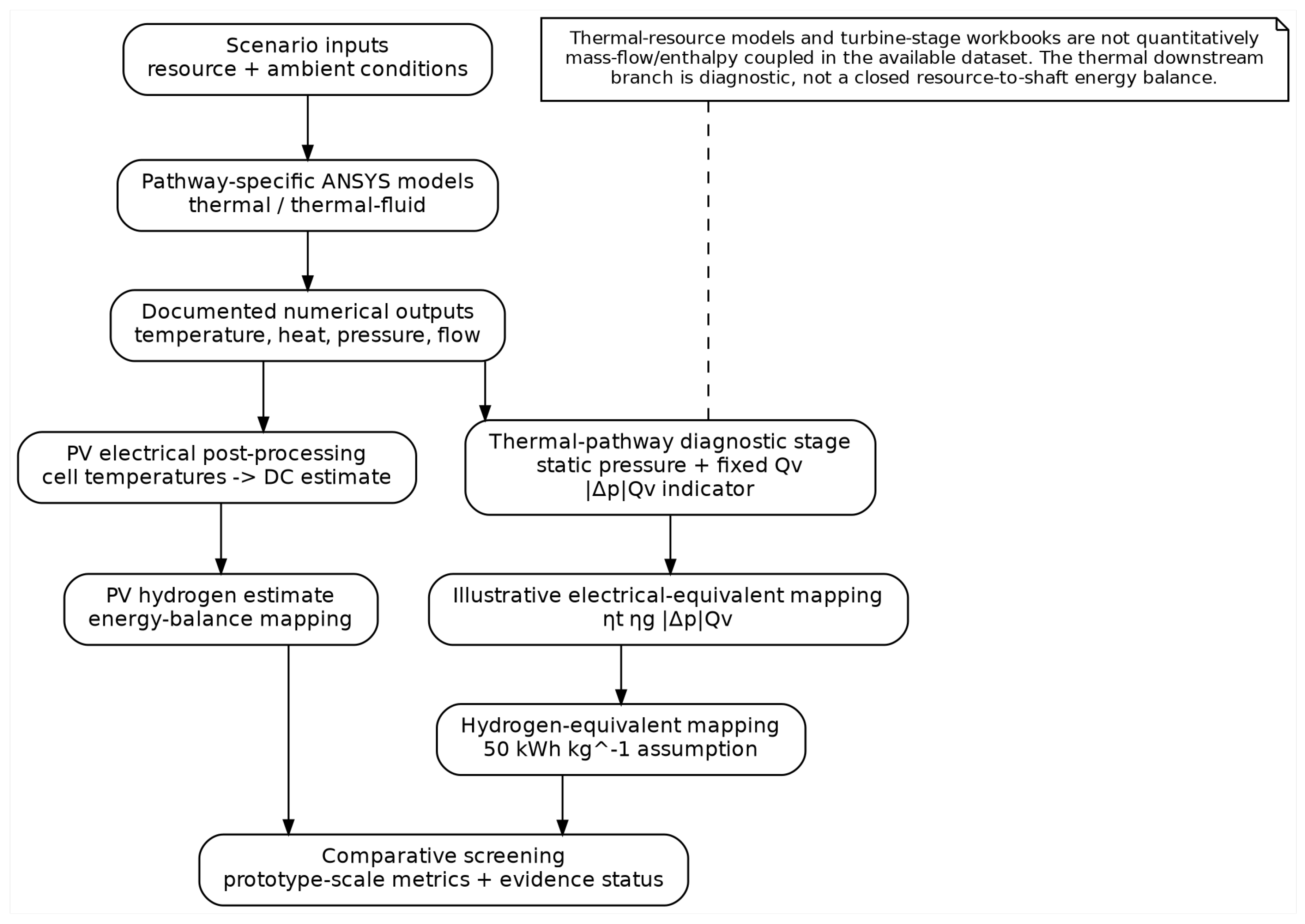
Figure 2.
PV DC power estimates by scenario from the final workbook. The exact final temperature coefficient equation is unavailable and is therefore not reconstructed.
Figure 2.
PV DC power estimates by scenario from the final workbook. The exact final temperature coefficient equation is unavailable and is therefore not reconstructed.
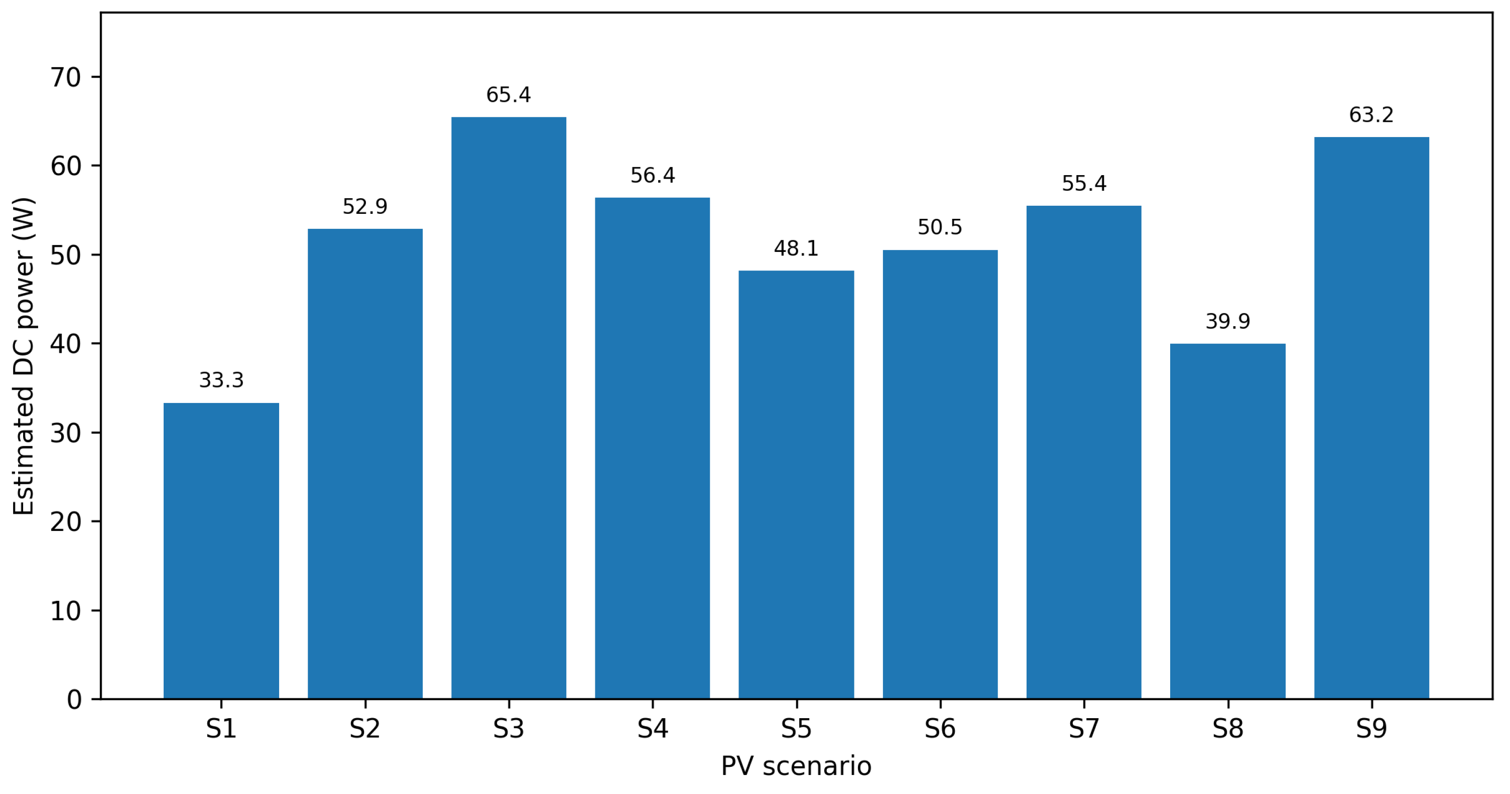
Figure 3.
CSP imposed receiver heat flux and reported heat transfer output. The receiver flux is a boundary condition representing the optical stage at reduced order; no ray tracing solution is implied.
Figure 3.
CSP imposed receiver heat flux and reported heat transfer output. The receiver flux is a boundary condition representing the optical stage at reduced order; no ray tracing solution is implied.
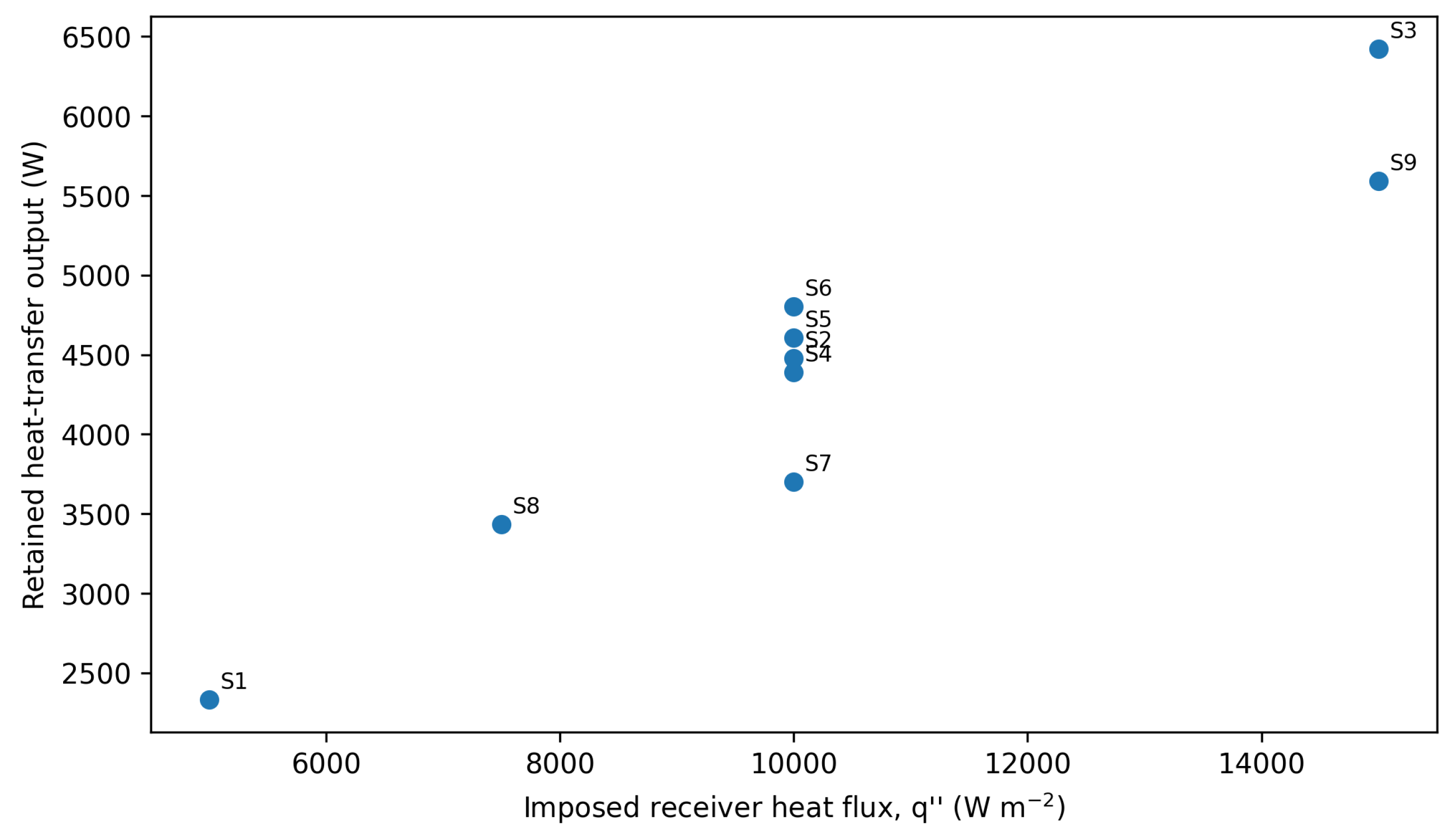
Figure 4.
Selected numerical fields. Color scales are independent between panels. WHR-S5 is a high-flow sensitivity/stress case, not a representative annual WHR condition.
Figure 4.
Selected numerical fields. Color scales are independent between panels. WHR-S5 is a high-flow sensitivity/stress case, not a representative annual WHR condition.
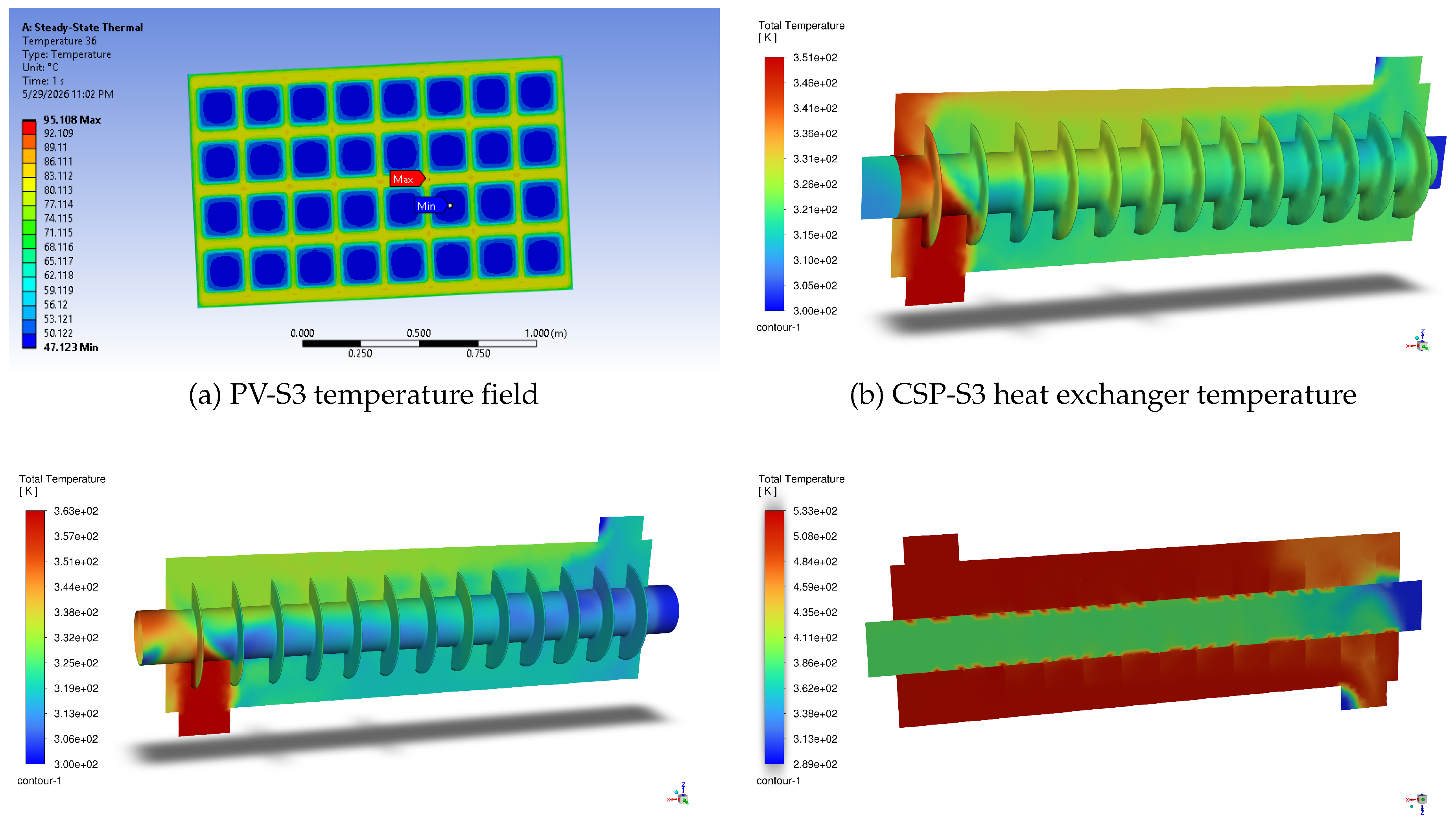
Figure 5.
Electrical equivalent indicator derived from the pressure-flow diagnostic for each pathway-specific scenario. Individual bars are not connected because scenario indices represent different physical perturbations in CSP, geothermal and WHR. The common factor reproduces the documented downstream scaling; the ordinate is a diagnostic mapping, not measured or CFD-resolved turbine electrical output.
Figure 5.
Electrical equivalent indicator derived from the pressure-flow diagnostic for each pathway-specific scenario. Individual bars are not connected because scenario indices represent different physical perturbations in CSP, geothermal and WHR. The common factor reproduces the documented downstream scaling; the ordinate is a diagnostic mapping, not measured or CFD-resolved turbine electrical output.
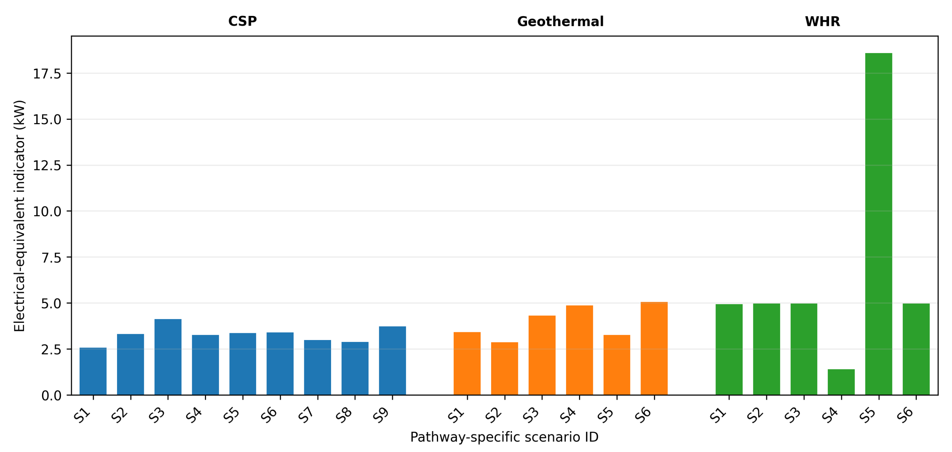
Figure 6.
Effect of WHR-S5 on the pathway mean. Excluding the high-flow stress case reduces the mean electrical equivalent indicator from 6.635 to 4.245 kW.
Figure 6.
Effect of WHR-S5 on the pathway mean. Excluding the high-flow stress case reduces the mean electrical equivalent indicator from 6.635 to 4.245 kW.
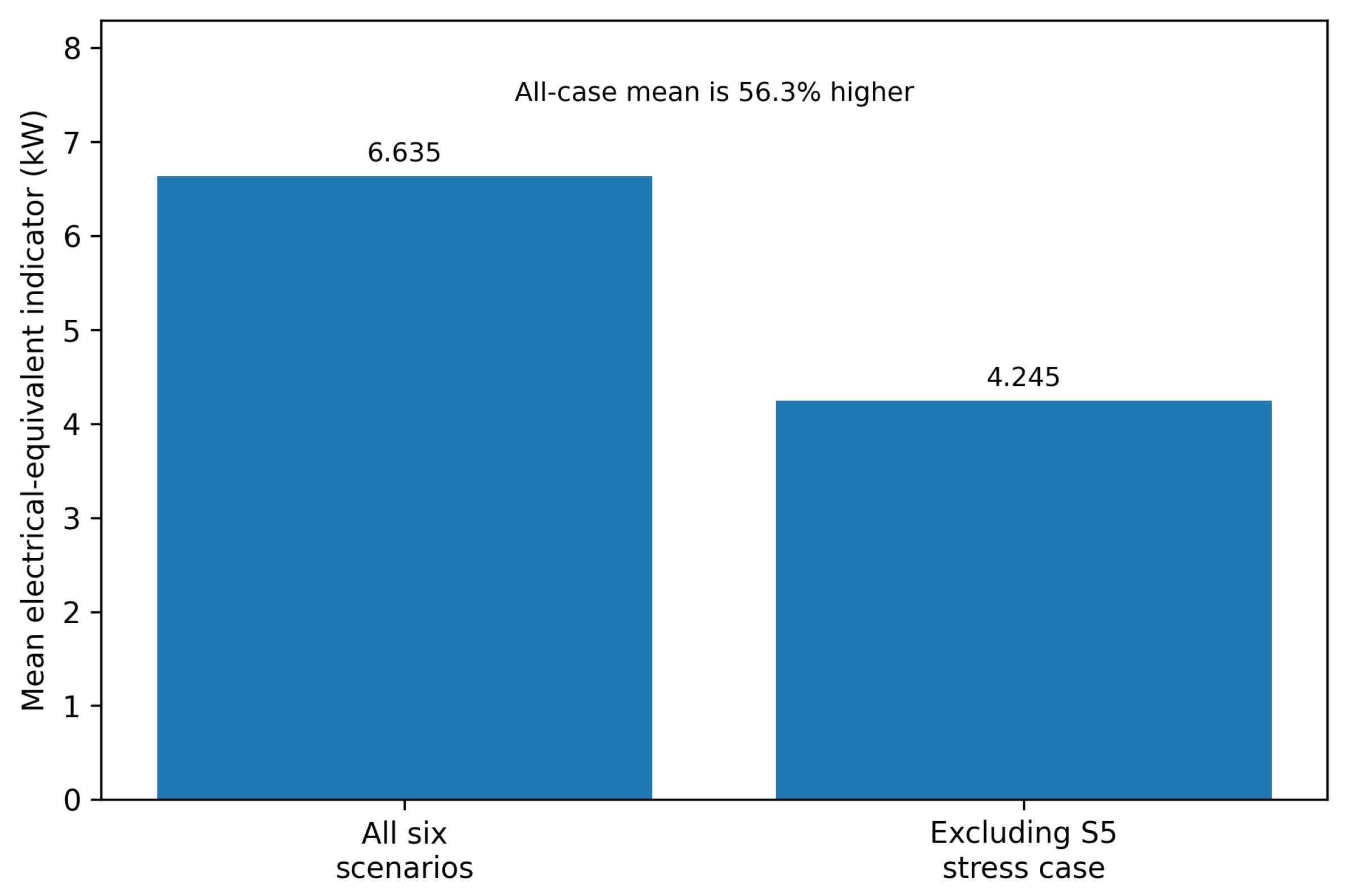
Table 3.
Reproducibility status of the numerical models. Missing numerical details are not replaced by typical CFD settings.
Table 3.
Reproducibility status of the numerical models. Missing numerical details are not replaced by typical CFD settings.
| Item | Documented evidence | Unresolved information |
|---|---|---|
| Software chain | ANSYS Workbench executable path v241; MATLAB launch scripts; MATLAB/Python post-processing. | Exact Fluent build metadata beyond the available Workbench path. |
| Model classes | Steady-State Thermal is documented for solid thermal calculations; Fluent is used for thermal-fluid stages; system-level data transfer is present in the available workflow. | Exact steady/transient formulation of each Fluent case. |
| Scenario boundary parameters | PV irradiance/heat flux, ambient temperature and convection coefficient; CSP imposed receiver heat flux, ambient temperature and convection coefficient; geothermal/WHR hot- and cold-side temperatures and velocities. | Exact face-by-face boundary condition type mapping for all domains. |
| Turbulence inputs | Turbulence intensity and viscosity ratio parameters are present in the launcher inputs. | Turbulence closure model (e.g., no defensible basis to state k– or k– SST), wall treatment and near-wall resolution. |
| Mesh | Simplified geometries and mesh generation are described qualitatively. | Cell/element counts, mesh topology, inflation layers, quality metrics and refinement sequence. |
| Solver numerics | No complete numerical record is available. | Pressure–velocity coupling, spatial discretization, initialization, residual thresholds, mass/energy imbalance and iteration histories. |
| Verification/validation | Scenario sensitivity and qualitative physical plausibility can be assessed from the available outputs. | Grid independence, quantitative benchmark validation and experimental validation. |
Table 4.
PV scenario inputs used in the comparison.
| ID | Scenario | G (W ) | (∘C) | h (W ) | Perturbation |
|---|---|---|---|---|---|
| S1 | Low solar | 500 | 25 | 10 | reduced irradiance |
| S2 | Normal | 800 | 25 | 10 | baseline |
| S3 | High irradiance | 1000 | 25 | 10 | high solar input |
| S4 | Cold ambient | 800 | 10 | 10 | low ambient temperature |
| S5 | Hot desert | 800 | 45 | 10 | high ambient temperature |
| S6 | No wind | 800 | 25 | 5 | weak convection |
| S7 | Wind cooling | 800 | 25 | 25 | strong convection |
| S8 | Dust/soiling | 600 | 25 | 10 | reduced incident input |
| S9 | Harsh desert | 1000 | 45 | 25 | high flux and hot ambient |
Table 5.
CSP scenario inputs. The receiver heat flux is imposed as a reduced-order representation of the optical stage; ray tracing was not performed.
Table 5.
CSP scenario inputs. The receiver heat flux is imposed as a reduced-order representation of the optical stage; ray tracing was not performed.
| ID | Scenario | (W ) | (∘C) | h (W ) | Perturbation |
|---|---|---|---|---|---|
| S1 | Low solar | 5000 | 25 | 10 | low imposed flux |
| S2 | Nominal | 10000 | 25 | 10 | baseline |
| S3 | High solar | 15000 | 25 | 10 | high imposed flux |
| S4 | Cold ambient | 10000 | 10 | 10 | low ambient temperature |
| S5 | Hot ambient | 10000 | 45 | 10 | high ambient temperature |
| S6 | No wind | 10000 | 25 | 5 | weak convection |
| S7 | Windy | 10000 | 25 | 25 | strong convection |
| S8 | Dust loss | 7500 | 25 | 10 | reduced imposed flux |
| S9 | Harsh desert | 15000 | 45 | 25 | high flux and hot ambient |
Table 6.
Fixed CSP launcher/property inputs documented in the parameter files. The primary scenario and geometry table consistently records a 0.002 m tube wall thickness; a separate legacy export field labelled tube thickness contains 0.010 m and is treated as ambiguous metadata rather than as the geometry input.
Table 6.
Fixed CSP launcher/property inputs documented in the parameter files. The primary scenario and geometry table consistently records a 0.002 m tube wall thickness; a separate legacy export field labelled tube thickness contains 0.010 m and is treated as ambiguous metadata rather than as the geometry input.
| Parameter | Documented value | Interpretation/status |
|---|---|---|
| Fluid inlet velocity | 0.50 m | Fixed launcher input |
| Fluid density | 1008 kg | Fixed launcher property |
| Fluid heat capacity | 1563 J | Fixed launcher property |
| Fluid thermal conductivity | 0.118 W | Fixed launcher property |
| Fluid dynamic viscosity | 0.0714 Pa s | Fixed launcher property |
| Initial fluid pressure | 14,280 Pa | Fixed launcher initialization field |
| Initial fluid temperature | 300 K | Fixed launcher initialization field |
| Surface emissivity | 0.85 | Fixed radiation input |
| Tube density | 8000 kg | Fixed launcher property |
| Tube heat capacity | 500 J | Fixed launcher property |
| Tube thermal conductivity | 16.2 W | Fixed launcher property |
| Fluid diameter | 0.020 m | Fixed launcher geometry parameter |
| Tube wall thickness | 0.002 m | Both tube_thickness and tube_thickness_geometry are 0.002 m in the scenario parameter file; the separate legacy P92 field at 0.010 m is excluded from geometry-sensitive interpretation until its meaning is clarified |
| Turbulence inputs | 1; 1 | Stored intensity and viscosity ratio inputs; unit/convention and closure model are unresolved |
Table 7.
Geothermal and WHR thermal resource scenario inputs. WHR-S6 contains the same cold-side velocity as WHR-S2 despite its scenario label; this discrepancy is not corrected without source evidence.
Table 7.
Geothermal and WHR thermal resource scenario inputs. WHR-S6 contains the same cold-side velocity as WHR-S2 despite its scenario label; this discrepancy is not corrected without source evidence.
| Path | Scenario | (K) | (m ) | (m ) |
|---|---|---|---|---|
| Geo | S1 Low temperature | 363.15 | 0.50 | 0.50 |
| Geo | S2 Medium temperature | 393.15 | 0.50 | 0.50 |
| Geo | S3 High temperature | 423.15 | 0.50 | 0.50 |
| Geo | S4 Low brine flow | 393.15 | 0.25 | 0.50 |
| Geo | S5 High brine flow | 393.15 | 1.00 | 0.50 |
| Geo | S6 High cold-flow absorption | 393.15 | 0.50 | 1.00 |
| WHR | S1 Low-grade heat | 423.15 | 3.0 | 0.50 |
| WHR | S2 Medium-grade heat | 523.15 | 3.0 | 0.50 |
| WHR | S3 High-grade heat | 623.15 | 3.0 | 0.50 |
| WHR | S4 Low source flow | 523.15 | 1.5 | 0.50 |
| WHR | S5 High source flow | 523.15 | 6.0 | 0.50 |
| WHR | S6 High cooling flow (source label) | 523.15 | 3.0 | 0.50 |
Table 8.
Thermal pathway indicators derived from the pressure-flow diagnostic. is not validated turbine-generator output.
Table 8.
Thermal pathway indicators derived from the pressure-flow diagnostic. is not validated turbine-generator output.
| Pathway | range (kPa) | ( ) | range (kW) | Mean (kW) |
|---|---|---|---|---|
| CSP | 4.771–7.676 | 1.8044 | 8.608–13.851 | 3.287 |
| Geothermal | 5.330–9.428 | 1.8044 | 9.617–17.011 | 3.964 |
| WHR, all scenarios | 2.599–34.624 | 1.8044 | 4.689–62.475 | 6.635 |
| WHR, S5 excluded | 2.599–9.253 | 1.8044 | 4.689–16.697 | 4.245 |
Disclaimer/Publisher’s Note: The statements, opinions and data contained in all publications are solely those of the individual author(s) and contributor(s) and not of MDPI and/or the editor(s). MDPI and/or the editor(s) disclaim responsibility for any injury to people or property resulting from any ideas, methods, instructions or products referred to in the content. |
© 2026 by the authors. Licensee MDPI, Basel, Switzerland. This article is an open access article distributed under the terms and conditions of the Creative Commons Attribution (CC BY) license (http://creativecommons.org/licenses/by/4.0/).
Copyright: This open access article is published under a Creative Commons CC BY 4.0 license, which permit the free download, distribution, and reuse, provided that the author and preprint are cited in any reuse.