Preprint
Article

This version is not peer-reviewed.

When and How Flocks Break: Field of View and Density in the Vicsek Model

Submitted:

13 August 2026

Posted:

14 August 2026

You are already at the latest version

Abstract

Collective motion happens when many individuals move together using only local rules, with no leader. The Vicsek model captures this through a noise-driven transition from order to disorder, but it usually assumes that agents can see in every direction and that the crowd stays at one fixed density, neither of which is realistic. We ask whether an agent's field of view (\(\alpha\)) and the population density (N) work together to shape the character of this transition, meaning how sharply a flock falls apart rather than only at what noise level it does. We add a forward vision cone to the Vicsek model and run a full sweep of 4 field-of-view angles, 3 densities, and 11 noise levels, with 30 seeds each (3960 runs). For each run we fit a logistic curve to the order parameter as noise rises and read off two numbers: the steepness \(k\) and the break-point \(\eta_c\). A two-way ANOVA shows that field of view and density work together to set where the flock breaks, but not how sharply it breaks; sharpness is shaped by density and field of view separately, with no interaction between them. Our hypothesis predicted an interaction on the sharpness, so it is only partly supported: density does not make up for a narrow field of view the way we expected. The result separates two parts of robustness that are easy to confuse and shows which one sensing range actually affects.

Keywords: 
;  ;  ;  ;  ;  ;  ;  ;  ;  ;  ;  

1. Introduction

Collective intelligence looks at how simple agents following local rules end up producing coordinated group behaviour [6,7,8]. Schools of fish, flocks of birds, and swarms of insects move as one body even though no individual is in charge; the order comes from each one reacting only to its nearby neighbours [3,8]. Understanding when this order appears, and just as importantly when it breaks down, helps explain natural group behaviour and helps in designing engineered swarms such as drone fleets, which have to keep working with imperfect sensors and changing group sizes.
The standard minimal model for this is the Vicsek model [8], where particles move at a constant speed and keep adjusting their heading to match the average heading of their nearby neighbours, with some random noise added. As the noise goes up, the system passes through a transition from ordered, coordinated motion into disorder. Where this transition sits is well studied, but its character is debated: whether the collapse is sudden (first-order) or gradual (second-order) depends on the system size and the modelling choices [2,5]. This difference matters in a way the location alone does not. A flock that loses order gradually can recover once conditions improve, while one that collapses suddenly may scatter for good. For animals avoiding predators, and for swarms working near their sensing limits, whether coordination fails gently or all at once is a question of robustness, not just of the exact noise level where order is lost.
The standard model assumes agents see in all directions and works at a single density. Both assumptions are unrealistic: real animals have limited visual fields [3], and real swarms run at different densities and sensor coverages. These two limits are also linked. A narrow cone in a dense crowd may still see many neighbours, while a wide cone in a sparse group may see very few, so the two factors could combine in a way that neither does on its own. We therefore ask: in the Vicsek model, do an agent’s field-of-view angle α and the density N work together to determine the character of the order–disorder transition? The model is the Vicsek model with an added forward vision cone [4]; the manipulated variables are the field-of-view angle α and the density N; and the measured outcome is the transition character, captured by two numbers taken from the order parameter φ : the steepness k of the collapse (our main measure of character) and the break-point η c where it happens (a secondary measure of location).
We expected a combined, non-additive effect based on the idea of effective neighbourhood size: the number of neighbours an agent really aligns with equals how many are nearby (set by density) times the share of them inside its vision cone (set by field of view). At low density there are few neighbours nearby, so narrowing the cone changes little and the transition should stay gradual no matter what α is. At high density there are many neighbours, so the cone becomes the limiting factor, and even a narrow field of view should still catch enough neighbours to keep the collapse sharp. So the effect of field of view on transition character should depend on density: a significant α × N interaction. This is testable and can be rejected: it fails if there is no such interaction, or if high density does not keep the transition sharp under a narrow cone.
We chose the Vicsek model because it is the simplest model in which an order–disorder transition comes purely from local alignment, so anything we find can be traced back to the alignment rule rather than to extra complexity. Field of view is a clean, biologically sensible change to the sensing rule that leaves the rest of the dynamics untouched, and density connects to it through effective neighbourhood size, which makes their combined effect hard to predict in advance. We thought about changing the interaction radius r instead of density, but radius and density both change how many neighbours an agent has, so they would be tangled together; field of view gives an independent way to limit sensing that radius does not. We also thought about changing only field of view and asking how it shifts the transition location, but that effect is fairly easy to predict in advance and would not have been a real open question. As we show, field of view and density do work together, but on where the flock breaks rather than how sharply, so the hypothesis is only partly supported. The rest of the report lays out the method, shows the results, and explains this split, coming back throughout to whether the two factors act together or separately.

2. Methodology

Three papers shape our approach. Vicsek et al. [8] give us the model itself: the constant-speed alignment rule, the order parameter φ , and the noise-driven transition we study. Grégoire and Chaté [5] showed that the sharpness of this transition is not fixed but depends on system size and setup, which is exactly why we measure sharpness for each condition instead of assuming it, and it is the reason we use a steepness metric. Couzin et al. [3] showed that real animals sense through limited zones rather than in all directions, and that the shape of their sensing changes who influences whom, which is the biological reason for adding a vision cone and changing its width. Together these give us a model, a reason to measure rather than assume sharpness, and a justification for the variable we change.
Model and agent design. Each agent has a position and a heading and moves at a fixed speed v 0 . The update at each step has four parts. State: the agent stores its position ( x , y ) and heading θ . Perception: the agent finds candidate neighbours within a radius r, then keeps only those inside its forward vision cone of width α . Decision: the agent takes the average heading of the neighbours it can see and adds a random nudge drawn evenly from [ η / 2 , η / 2 ] . Action: the agent turns to the new heading and moves one step at speed v 0 . The world is a square with wrap-around edges, so an agent that leaves one side comes back on the other, which removes edge effects. These four parts make up one rule that every agent applies on its own at the same time each step, and all the group behaviour we study comes from repeating this single local rule.
Field-of-view module. The vision cone is just an angle check added on top of the normal distance check [4]. A neighbour j counts for agent i only if it passes both tests: j is within radius r of i, and the angle between i’s heading and the direction toward j is at most α / 2 . At α = 360 the angle check is always true and the model is exactly standard Vicsek; smaller α removes more neighbours outside the forward arc, so a narrow cone makes an agent blind to companions behind and beside it even when they are close. This is the only change we make to the standard model, which means any effect we see can be put down to limited sensing rather than to some other choice. A cone of this kind has been studied before, but along a different axis: Durve and Sayeed [4] hold the noise fixed and sweep the view angle itself as the control parameter, reporting that ordered motion survives down to remarkably narrow angles, that the system undergoes a first-order transition to disorder at a certain angle, and that narrowing the cone can even raise the order in the system. Our design runs the other way round, sweeping noise at a fixed view angle and crossing that sweep with density, so the two studies cut the same ( α , η ) plane in perpendicular directions and their result that a narrow cone can help is not in conflict with ours that a wide cone holds order to higher noise.
Order parameter. The order parameter φ is the length of the average unit velocity over all N agents, ranging from 0 to 1. When every agent moves the same way the arrows add up and φ 1 ; when headings are random they cancel and φ 0 . Values in between mean partial alignment. We compute φ each frame and average it over the later part of each run, so early start-up wobble does not affect the measurement.
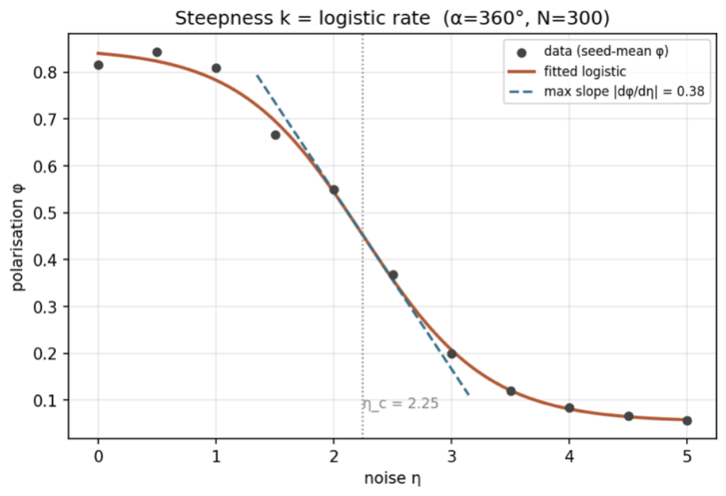
Measuring transition character. We fit a logistic (S-shaped) curve to the φ -versus- η data and read off two numbers from the fit. The steepnessk is the rate parameter of the fitted logistic, which controls how fast φ drops through the transition (a big k means a sudden, first-order-like collapse; a small k means a slow, second-order-like fade). The maximum slope of the curve is a related quantity, equal to A k / 4 for a logistic of amplitude A, and we use it only to illustrate the fit. The break-point η c is the noise level at the middle of the curve. Steepness is our main measure because the question is about transition character; the break-point is a secondary measure of location. Turning each curve into these two numbers is what makes the vague words “steep” and “gradual” precise and repeatable: anyone applying the same fit to the same data would get the same values.
Experimental setup. We ran a full factorial design crossing 4 field-of-view angles ( α { 90 , 180 , 270 , 360 } ) with 3 densities ( N { 50 , 150 , 300 } agents in a fixed 750 × 750 world), giving 12 conditions. For each condition we swept the noise η across 11 levels and repeated everything with 30 separate random seeds, for 4 × 3 × 11 × 30 = 3 , 960 runs in total. We held the world size ( 750 × 750 , wrap-around), the speed ( v 0 = 2.0 ), the radius ( r = 50 ), and the run length (400 frames, with the first 200 dropped as warm-up) constant. Noise η is not a manipulated factor but the axis we sweep to find and measure the transition inside each condition. We fit the logistic curve separately for each seed within each condition, which gives one steepness k and one break-point η c per seed, so 360 fits in total ( 12 × 30 ). Of those 360 fits, 354 converged; the 6 that failed all came from the sparsest condition, where the flock barely orders at all. We then run a two-way ANOVA on these per-seed values, with α (4 levels) and N (3 levels) as the two factors, once for k and once for η c . ANOVA fits this design because it has two categorical factors with many independent values per cell, and the α × N interaction term is exactly our hypothesis: a significant interaction means the effect of field of view depends on density.

3. Experiments

3.1. Experimental Setup

The setup is given at the end of the Methodology section: a full sweep of α and N, with noise η as the control axis, 30 seeds per condition, and a two-way ANOVA on the per-seed logistic measures k and η c . Figure 1 shows the two states the experiment moves between: at low noise the agents lock into one shared direction, and at high noise they scatter. The whole study is basically a map of how the noise level where a flock drops from the first state into the second, and how sharply it drops, change with field of view and density. We show the results as graphs and interpret them, leaving the overall conclusions about the data for the end of this section.

3.2. Results

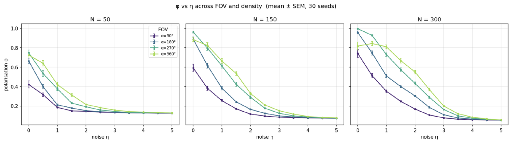
Figure 2 shows φ against noise for every condition, with one panel per density. Order drops as noise rises everywhere, which is expected. Two other things stand out: higher density keeps order higher and holds it to higher noise, and within each panel a wider field of view also holds order to higher noise than a narrow one. At very low noise the conditions all sit near full order and their ordering is mostly down to seed-to-seed randomness, so the real separation shows up in the middle noise range rather than at η = 0 . The bottom line is that both factors clearly delay the collapse, which sets up the question this study answers: do they delay it together or separately?
Figure 3 shows how we read the two numbers from a single condition: the logistic fit follows the seed-mean φ closely, its rate parameter gives the steepness k, and its middle gives the break-point η c . This turns each curve into the two numbers we analyse, and reading both from the same fit lets us ask separately whether the factors control where the flock breaks and how sharply it does.
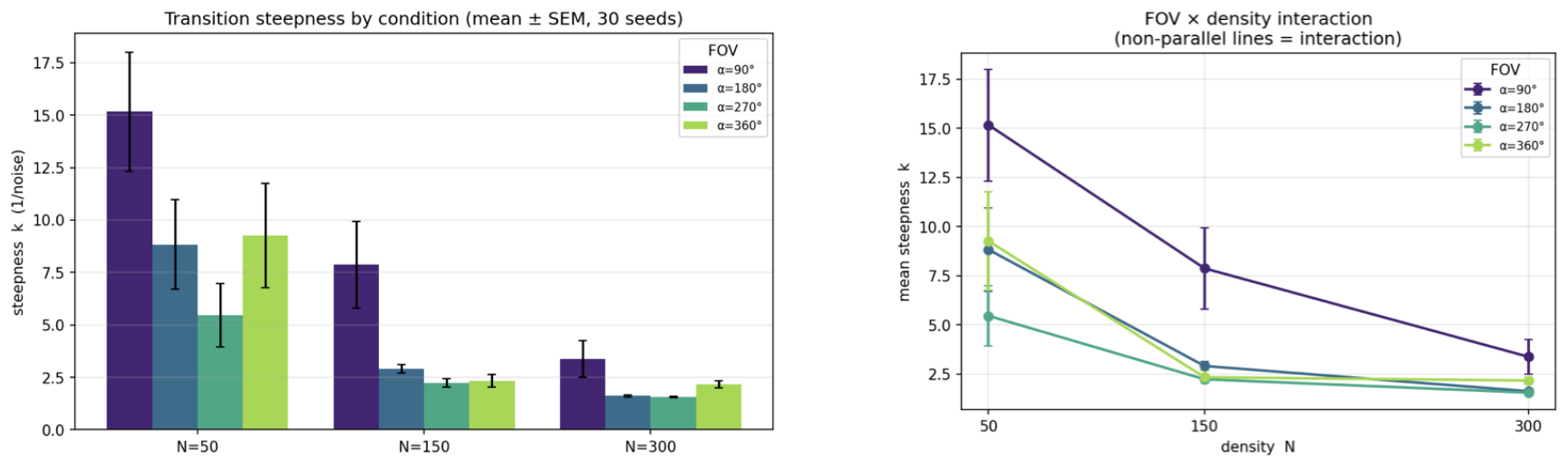
Figure 4 shows steepness across conditions, both as grouped bars and as an interaction plot. Steepness drops a lot with density: collapses are much steeper at N = 50 than at N = 300 , so denser flocks actually lose order more gradually. The interaction plot shows the field-of-view lines spreading apart at low density, where the narrowest cone gives the steepest collapse, but coming back together and running roughly parallel at high density. This spread at low density comes with very large error bars: the sparse system barely forms a flock, so its fitted steepness jumps around a lot from seed to seed and is not reliable. The visual hint of an interaction is therefore sitting exactly where our measure is weakest, which is why the formal test, not the eye, has to decide whether the factors really act together on sharpness.
Table 1 gives the two-way ANOVA for both measures. For steepness k, both main effects are significant but the α × N interaction is not ( F ( 6 , 342 ) = 1.35 , p = 0.236 ): how sharply the flock breaks is set by density and by field of view separately, with no sign that they act together. For the break-point η c , all three terms are significant, including a strong interaction ( F ( 6 , 342 ) = 11.36 , p < 0.001 ): where the flock breaks depends on field of view and density together. The formal test therefore overturns the visual impression from the steepness interaction plot and confirms the opposite pattern for the break-point.
Putting it together, the experiments split apart two parts of the transition that are easy to mix up. Field of view and density together set the noise level where order collapses, but how sudden that collapse is is set by the two factors separately, with no sign that they combine. The eye-catching interaction in steepness at low density is not backed up by the statistics and lands exactly in the regime where our measure is least reliable, so we do not treat it as real. The clean result is a split: the two factors cooperate on where the flock breaks but act on their own on how sharply it breaks.

4. Conclusion

We set out to find whether an agent’s field of view and the density work together to shape the character of the order–disorder transition in the Vicsek model. The answer is that they work together to set where the transition happens but not how sharply it happens: how sudden the collapse is depends on density and field of view separately, but the two do not combine, while for the location field of view and density join up to move where the transition sits. The break-point result fits the effective-neighbourhood-size idea that motivated the study, since both factors raise how many neighbours an agent aligns with and so together raise the noise the flock can take before breaking; but the sharpness of the collapse is not driven by that same quantity, so the two parts of the transition come from partly different mechanisms.
Our hypothesis predicted the interaction would show up in the sharpness. It showed up in the location instead, so the hypothesis is partly supported: the mechanism is real and visible in where the flock breaks, but it does not appear in how sharply it breaks the way we expected. This fits with the literature: we reproduce the transition described by Vicsek, we see the setup-dependent fragility of its sharpness noted by Grégoire and Chaté in our shaky low-density case, and we match the strong effect of limited sensing on who interacts with whom described by Couzin et al. So the contribution is less a confirmation of our original guess than a clarification: where a flock breaks and how sharply it breaks are separate properties that respond to sensing and crowding in different ways, which is a sharper statement than treating robustness as a single thing.
A few limitations bound what we can claim. The steepness measure is unreliable at the lowest density, where the flock barely orders and a handful of fits failed; the high, jumpy steepness values there come from the unstable fit in that regime rather than from a real sharper transition, so we read the low-density steepness with caution. Density and agent count are also tied together in our design, since we fixed the world size and only changed N, so we cannot fully separate “denser” from “more agents”; this is a real limitation, but the density trend cannot just be a simple finite-size effect, because a finite-size effect would push toward a sharper transition with more agents, while we see the opposite, a more gradual one. A related caveat is that effective neighbourhood size is an assumption of the metric model we chose rather than an established fact about real flocks: Ballerini et al. [1] found that starlings interact with a roughly fixed number of neighbours, six to seven, rather than with every bird inside a fixed metric radius, and argued that this topological rule is what holds a flock together when density changes. If interaction is topological, neighbour count does not scale with density at all, so the density leg of our mechanism is specific to the metric Vicsek model and should not be read as a claim about real animal groups. We also used only one kind of noise (added to the heading) and a fairly narrow set of parameter values, and we inferred sharpness from steepness rather than confirming it directly.
The biggest challenge was making “character” measurable in the first place: turning the loose idea of a sudden versus gradual collapse into a repeatable number meant committing to a fitted measure, and the sparse case showed how shaky that fit gets when there is barely any order to fit. Telling apart a real interaction from one that only looks convincing on a plot was the main interpretive difficulty, and it is why we trusted the formal test over the look of the graphs. The clearest next step is to make the sharpness measure steadier by sampling more noise levels around the break-point and running the sparsest cases longer, so character can be measured reliably where it currently cannot. A natural follow-up is to confirm the type of collapse directly with a hysteresis test, sweeping noise up and then back down, instead of inferring it from steepness. More ambitiously, widening the parameter ranges to very high densities and very narrow cones, and trying other kinds of noise such as perceptual noise, would map out the edges of the effects we found and test how far the effective-neighbourhood-size idea really reaches.

References

  1. Ballerini, M.; Cabibbo, N.; Candelier, R.; Cavagna, A.; Cisbani, E.; Giardina, I.; Lecomte, V.; Orlandi, A.; Parisi, G.; Procaccini, A.; Viale, M.; Zdravkovic, V. Interaction ruling animal collective behavior depends on topological rather than metric distance: Evidence from a field study. Proc. Natl. Acad. Sci. 2008, 105(4), 1232–1237. [Google Scholar] [CrossRef] [PubMed]
  2. Chaté, Hugues; Ginelli, Francesco; Grégoire, Guillaume; Raynaud, Franck. Collective motion of self-propelled particles interacting without cohesion. Phys. Rev. E 2008, 77(4), 046113. [Google Scholar] [CrossRef] [PubMed]
  3. Couzin, Iain D; Krause, Jens; James, Richard; Ruxton, Graeme D; Franks, Nigel R. Collective memory and spatial sorting in animal groups. J. Theor. Biol. 2002, 218(1), 1–11. [Google Scholar] [CrossRef] [PubMed]
  4. Durve, Mihir; Sayeed, Ahmed. First-order phase transition in a model of self-propelled particles with variable angular range of interaction. Phys. Rev. E 2016, 93(5), 052115. [Google Scholar] [CrossRef] [PubMed]
  5. Grégoire, Guillaume; Chaté, Hugues. Onset of collective and cohesive motion. Phys. Rev. Lett. 2004, 92(2), 025702. [Google Scholar] [CrossRef] [PubMed]
  6. Reynolds, Craig W. Flocks, herds and schools: A distributed behavioral model. ACM SIGGRAPH Comput. Graph. 1987, 21(4), 25–34. [Google Scholar] [CrossRef]
  7. Vicsek, Tamás; Zafeiris, Anna. Collective motion. Phys. Rep. 2012, 517(3–4), 71–140. [Google Scholar] [CrossRef]
  8. Vicsek, Tamás; Czirók, András; Ben-Jacob, Eshel; Cohen, Inon; Shochet, Ofer. Novel type of phase transition in a system of self-driven particles. Phys. Rev. Lett. 1995, 75(6), 1226–1229. [Google Scholar] [CrossRef] [PubMed]
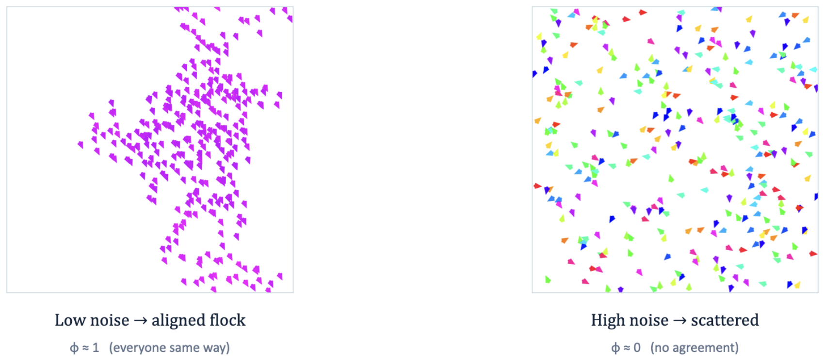
Figure 1. The two states the simulation moves between. Left: at low noise the agents line up into one coherent flock ( φ 1 ). Right: at high noise the headings turn random and the group scatters ( φ 0 ). The transition between these states is what we study.
Preprints 228218 g001
Figure 2. Order parameter φ versus noise η across field of view and density (mean ± SEM, 30 seeds). Panels: N = 50 , 150 , 300 ; colour: field-of-view angle α . Both higher density and wider field of view hold order to higher noise.
Preprints 228218 g002
Figure 3. How the two measures are read from one condition ( α = 360 , N = 300 ). The fitted logistic gives the rate parameter (steepness k) and the middle point (break-point η c ); the steepest slope shown is the related quantity A k / 4 .
Preprints 228218 g003
Figure 4. Transition steepness k by condition (mean ± SEM, 30 seeds). Left: grouped bars. Right: interaction plot, where non-parallel lines would suggest an interaction. The wide spread at N = 50 reflects unstable fits in the sparse case.
Preprints 228218 g004
Table 1. Two-way ANOVA for steepness k (primary) and break-point η c (secondary). Residual d f = 342 .
Measure Effect F df p
Steepness k FOV ( α ) 8.01 3, 342 < 0.001
Density (N) 27.74 2, 342 < 0.001
α × N 1.35 6, 342 0.236
Break-point η c FOV ( α ) 133.9 3, 342 < 0.001
Density (N) 152.0 2, 342 < 0.001
α × N 11.36 6, 342 < 0.001
Disclaimer/Publisher’s Note: The statements, opinions and data contained in all publications are solely those of the individual author(s) and contributor(s) and not of MDPI and/or the editor(s). MDPI and/or the editor(s) disclaim responsibility for any injury to people or property resulting from any ideas, methods, instructions or products referred to in the content.
Copyright: This open access article is published under a Creative Commons CC BY 4.0 license, which permit the free download, distribution, and reuse, provided that the author and preprint are cited in any reuse.