
Submitted:
13 August 2026
Posted:
14 August 2026
You are already at the latest version
Abstract
Geological CO₂ storage must operate within pressure and stress limits that preserve caprock, fault, and well integrity while sustaining climate relevant injection. Existing reviews often treat multiphysics simulation, machine learning, and physics informed learning separately, which obscures the different evidence required for stability screening, first slip, aseismic deformation, dynamic rupture, monitoring analytics, and containment consequences. This structured critical review integrates direct CO₂ storage observations, laboratory studies, injection analogues, multiphysics numerical methods, data driven machine learning, and scientific machine learning within a target specific evidence framework. We compare continuum, discontinuum, interface, and diffuse fracture formulations; one way, staggered, and monolithic coupling; field and laboratory validation; seismic, deformation, pressure, and fiber optic monitoring; and physics informed neural networks, neural operators, and reduced order models. The synthesis shows that pressure and deformation modeling and seismic signal processing are comparatively mature, whereas prospective fault slip and seismicity forecasting remain limited by uncertain in situ stress, fault connectivity, CO₂ conditioned friction, monitoring detection limits, model discrepancy, and scarce cross site validation. We propose task appropriate metrics, an explicit validation ladder, and a staged, human supervised digital twin roadmap. Machine learning and physics informed methods are most credible as bounded complements to verified simulators and monitoring systems, and operational readiness should be judged by uncertainty calibrated prospective evidence rather than algorithm novelty.
Keywords:
geological CO₂ storage
; fault reactivation
; induced seismicity
; geomechanics
; thermo hydro mechanical coupling
; machine learning
; physics informed machine learning
; digital twin
1. Introduction
1.1. Carbon Storage at Scale and the Geomechanical Constraint
Carbon capture and storage is one of the mitigation options required in pathways that reach net zero greenhouse gas emissions, particularly for process emissions and hard to abate industrial sectors. Deep saline formations and depleted hydrocarbon reservoirs offer the largest practical subsurface capacity, but storage performance cannot be judged by pore volume alone. The feasible injection envelope is constrained by injectivity, pressure interference, caprock integrity, well integrity, fault stability, brine displacement, and the ability to verify containment over operational and after injection periods. These constraints become increasingly important as projects progress from single demonstration wells to multiwell systems that inject at rates of millions of tonnes per year [1,2,3].
Pressure is the central operational variable linking storage capacity to geomechanical risk. Injection raises pore pressure in the storage interval, changes the effective stress carried by the rock skeleton, and induces poroelastic deformation within and beyond the CO₂ plume. Cold injection may also alter the stress field through constrained thermal contraction. If a connected fault is favorably oriented and sufficiently close to frictional failure, a relatively modest pressure perturbation may initiate slip. The same operation can therefore produce three very different outcomes: benign elastic deformation, stable or aseismic fault displacement, or dynamic rupture accompanied by detectable seismic radiation. Predicting which outcome occurs requires a model that is explicit about the target of prediction and about the uncertainty in stress, fault geometry, hydraulic connectivity, and constitutive behavior [4,5,6,7].
Observed seismicity at CO₂ storage projects has generally been small relative to prominent injection induced earthquakes associated with wastewater disposal and enhanced geothermal stimulation. This empirical record is reassuring but not sufficient to eliminate concern. The number of commercial storage projects is still limited compared with the diversity of possible structural settings, and small events may indicate either localized benign deformation or activation of structures that could influence injectivity and containment. Moreover, the societal and regulatory significance of an event does not depend solely on magnitude. Repeated microseismicity, unexpected uplift, pressure excursions, or evidence for flow along a previously unresolved structure can change the interpreted risk state of a project even when no damaging earthquake occurs [8,9,10].
1.2. Why Fault Slip Prediction Is Intrinsically Multiphysics
Fault reactivation is commonly introduced using the Mohr Coulomb criterion: slip is possible when shear traction exceeds frictional resistance on a plane. That statement is necessary but incomplete for storage operations. Multiphase flow controls the spatial and temporal distribution of pressure. Poroelasticity converts pressure changes into total stress changes. Temperature affects fluid density and viscosity and may create thermal stresses. Fault opening, closure, shear dilation, gouge compaction, and damage alter permeability, which feeds back on pressure propagation. Chemical reactions may change aperture, cohesion, and friction over longer time scales. The resulting problem is coupled, path dependent, and strongly affected by spatial heterogeneity [11,12,13].
The term “fault slip prediction” is also used too broadly. A static slip tendency calculation is not equivalent to forecasting a seismic event. A model that identifies the pore pressure at first yield does not necessarily predict the subsequent slip distance, rupture area, or radiated energy. A seismic detector that classifies a waveform after it has arrived is not an early warning model. A surrogate that reproduces simulator outputs within the training distribution is not a validated predictor for a different field site. These distinctions are important because the validation data, performance metrics, and acceptable uncertainty differ for each task.
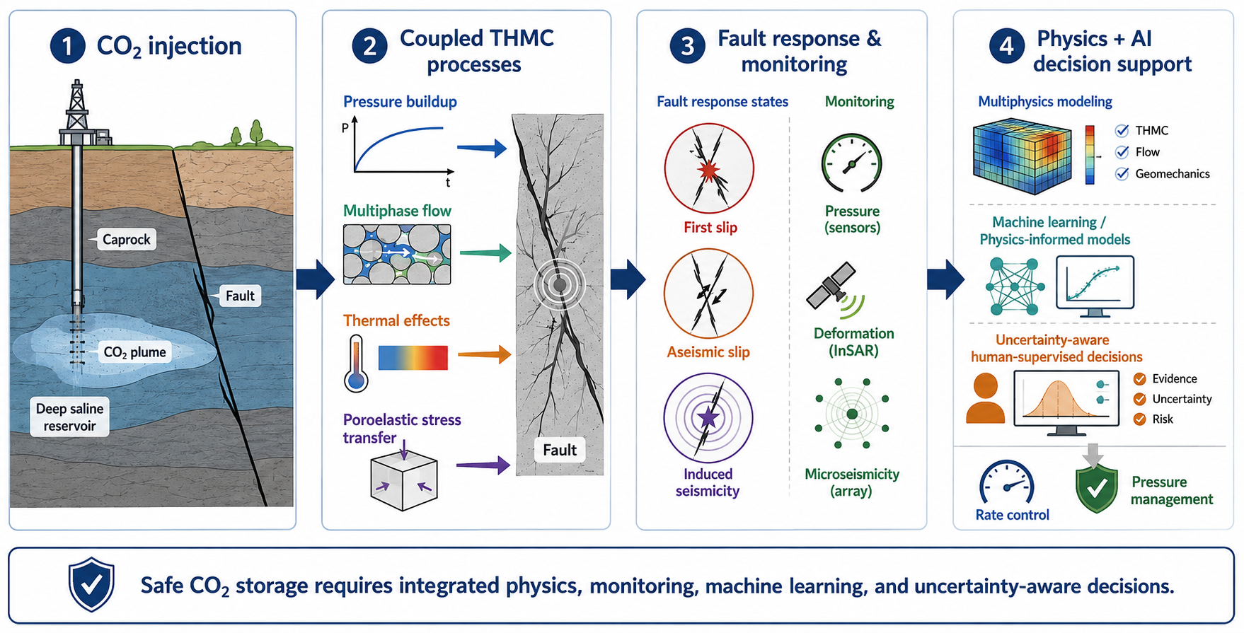
A credible prediction chain therefore begins with injection controls; propagates through reservoir state, fault stress, and constitutive response; predicts a defined slip regime; maps that response to observable signals; and supports an operational action. Monitoring closes the loop by updating model state and parameter distributions. Figure 1 summarizes this integration of storage system physics, monitoring evidence, scientific machine learning, and risk informed control.
1.3. Evolution of Modeling and Data Analysis
Early analyses of storage geomechanics relied on analytical poroelastic solutions, stress path calculations, and slip tendency screening. These methods remain valuable because they expose parameter dependence, allow rapid scenario evaluation, and provide verification cases for numerical codes. Their limitations are equally clear: they generally assume simple geometry, homogeneous material properties, linear response, and idealized boundaries. Site specific assessment requires numerical methods that represent three dimensional stratigraphy, fault networks, multiphase flow, nonlinear constitutive behavior, and operational well schedules [4,15,16].
A second development was the coupling of reservoir simulators with geomechanical codes. Finite volume or integrated finite difference flow solvers were linked to finite element or finite difference mechanics solvers through one way or iterated schemes. Such workflows enabled pressure and saturation fields to influence stress and deformation, and in more advanced implementations allowed deformation to update porosity and permeability. Dedicated multiphysics platforms, open source frameworks, and high performance computing have since enabled monolithic or tightly coupled thermal, hydraulic, and mechanical simulations, although computational cost and parameter uncertainty remain major constraints [17,18,19,20].
The rapid growth of high volume monitoring has created a parallel data science trajectory. Dense seismic arrays, distributed acoustic sensing, distributed temperature sensing, pressure gauges, tiltmeters, and satellite interferometry generate data at spatial and temporal resolutions that are difficult to process manually. Machine learning has improved event detection, phase picking, waveform classification, and extraction of low amplitude signals from noisy data. In laboratory friction experiments, statistical learning has also revealed reproducible relationships between continuous acoustic features and the evolving state of a fault. These developments are directly relevant to storage monitoring, but the strongest evidence often comes from natural seismicity, geothermal stimulation, or laboratory experiments rather than prospective CO₂ storage forecasts [21,22,23,24,25].
Scientific machine learning attempts to connect these trajectories. Physics informed neural networks impose governing equation residuals and boundary conditions during training. Neural operators learn mappings between input fields and solution fields across a family of problems. Reduced order and surrogate models approximate expensive simulators for uncertainty quantification, optimization, or data assimilation. These methods can be useful, but they should not be described as inherently more accurate, more physical, or more transferable than conventional solvers. Their credibility depends on the governing equations used, the fidelity of training simulations, the treatment of discontinuities, the sampling of parameter space, and independent validation [14,26,27,28].
1.4. Purpose and Contribution of This Review
This review integrates geomechanics, multiphase flow simulation, seismology, machine learning, and scientific computing around a common operational question: what information and modeling architecture are required to make fault reactivation predictions useful for storage decisions? Its novelty lies not in cataloguing each field separately, but in establishing a target specific evidence framework that connects physical models, monitoring observables, validation level, uncertainty, and decision use.
The review makes five contributions. First, it separates prediction targets that are frequently conflated: slip initiation, stable or aseismic deformation, dynamic rupture, seismicity rate response, monitoring classification, and containment consequence. Second, it evaluates numerical formulations by fault representation, constitutive assumptions, and coupling architecture rather than by software name. Third, it distinguishes code verification, calibration, retrospective field evaluation, cross site testing, and prospective forecasting. Fourth, it evaluates machine learning performance using task appropriate metrics, leakage safe partitions, probability calibration, and outside distribution behavior. Fifth, it proposes an auditable hybrid workflow in which verified physics, monitoring data, uncertainty quantification, scientific machine learning, and human oversight have explicit and limited roles.
The review focuses on deep saline formations and depleted hydrocarbon reservoirs. Evidence from enhanced geothermal systems, wastewater disposal, hydraulic stimulation, natural earthquakes, and laboratory friction experiments is used only when it clarifies a transferable mechanism or method. Such evidence is identified as analogue or controlled evidence rather than treated as proof that a CO₂ storage site will behave identically. The intended audience includes reservoir engineers, geomechanics specialists, seismologists, monitoring scientists, data scientists, regulators, and project developers.
2. Review Approach, Terminology, and Evidence Hierarchy
2.1. Structured Critical Review Method
The literature was assembled through iterative searches of Scopus, Web of Science, Google Scholar, ScienceDirect, OnePetro, and publisher databases, with a final update completed on 10 August 2026. Search blocks combined geological storage terms (for example, “CO₂ storage,” “geologic carbon sequestration,” and “CCS”) with geomechanical terms (“fault reactivation,” “induced seismicity,” “poroelasticity,” “fault slip,” and “caprock integrity”) and computational terms (“THM,” “THMC,” “coupled flow geomechanics,” “finite element,” “discrete element,” “machine learning,” “physics informed,” “surrogate,” and “neural operator”). Searches also targeted major storage sites and benchmark problems, and backward and forward citation chaining was applied to primary studies and major reviews.
Eligibility was assessed from topical relevance and then from the methodological information available in the full text. Priority was given to peer reviewed primary studies that defined the geometry, governing equations, constitutive assumptions, boundary conditions, data source, prediction target, and validation evidence. Foundational studies before 2015 were retained when they established effective stress theory, rate and state friction, numerical methods, or major field observations. Recent reviews were used to identify themes and sources, whereas software manuals were cited only for documented capabilities and not as evidence of predictive performance. Duplicate reports, nontechnical commentary, studies with insufficient methodological detail, and analogues lacking a clearly transferable mechanism were excluded from the evidential synthesis.
Each retained source was coded by evidence setting, direct CO₂ storage, controlled laboratory experiment, non CO₂ injection analogue, or synthetic/numerical benchmark, and by validation level: verification, laboratory validation, retrospective field evaluation, cross site evaluation, or prospective prediction. Because pressure, uplift, event location, magnitude, classification, and surrogate field errors are not interchangeable, no pooled accuracy or meta analytic effect size was calculated. Quantitative values are reported only when the original source defines the target, units, test data, and evaluation procedure sufficiently for interpretation. Table 1 summarizes the search scope, eligibility criteria, evidence classes, validation levels, synthesis method, and auditability rules used in this review.
Throughout Section 5 to 9, statements about method capability are therefore interpreted according to the highest evidence level demonstrated. A method shown on a synthetic benchmark is not described as field validated, and a laboratory or geothermal result is not treated as direct prospective evidence for CO₂ storage operations.
2.2. Terminology
In this review, fault reactivation means renewed shear or opening displacement on a preexisting discontinuity. Slip initiation is the onset of irreversible shear displacement according to a specified constitutive criterion. Aseismic slip is fault displacement that does not radiate sufficient high frequency elastic energy to be detected as an earthquake at the relevant network sensitivity. Dynamic rupture involves inertial acceleration, stress drop, and seismic radiation. Induced seismicity refers to detectable seismic events whose occurrence rate, timing, or location is influenced by human activity. Triggered seismicity is sometimes used when a small anthropogenic perturbation advances failure on a fault already close to instability; the distinction is conceptually useful but often difficult to establish observationally.
A forecast is a statement about a future quantity over a stated time window and spatial domain, made before the target observations are available. A retrospective prediction reconstructs past behavior using data that may have influenced model development. Calibration adjusts parameters to fit observations. Validation evaluates a model against independent observations not used in calibration. A surrogate approximates the input and output behavior of a simulator or experiment over a defined domain. A digital twin is used here in the strict sense of a continuously updated model and data system with explicit state estimation, uncertainty, decision rules, and governance; a static dashboard or a single calibrated model is not, by itself, a digital twin.
2.3. Evidence Hierarchy
Evidence becomes more demanding as a model is exposed to geological uncertainty. Code verification and canonical benchmarks test whether equations are solved correctly. Laboratory validation tests constitutive behavior under controlled boundary conditions. Retrospective field evaluation tests whether a model can reproduce independent observations from a real site. Cross site evaluation tests transferability. Prospective prediction evaluates whether a model can forecast observations that were not yet available. Figure 9 later formalizes this hierarchy. Throughout this review, claims about operational readiness are tied to the highest level of evidence demonstrated, not to the sophistication of the algorithm.
2.4. Review Limitations and Auditability
The literature is heterogeneous in geological setting, injection scale, constitutive assumptions, monitoring sensitivity, prediction target, and validation metric. Pooling numerical error, classification accuracy, seismicity forecasts, and field observations would create a false impression of comparability. The synthesis is therefore structured and critical rather than statistical, and quantitative comparisons are retained only where the original studies define commensurate targets and evaluation procedures.
Evidence used to establish a physical mechanism is distinguished from evidence used to claim predictive performance. A direct shear experiment can strongly support frictional weakening or dilation but weakly support site scale magnitude forecasting. A natural earthquake detector can demonstrate waveform processing capability without validating a prospective forecast of injection induced slip. Likewise, a history matched field model explains observations but is not an independent prediction unless the evaluated data were withheld from calibration.
Source traceability was treated as a publication quality requirement. Claims were checked against primary literature where feasible, and statements requiring an unavailable study level extraction record were removed or expressed qualitatively. The review does not claim a fixed number of included studies or a PRISMA compliant systematic corpus. Such a claim would require a registered protocol, duplicate removal log, full text exclusion table, extraction workbook, and formal study quality scores. Table 1 instead makes the present review’s scope, evidence coding, and limitations explicit and provides a basis for a future registered evidence map.
3. Defining the Prediction Problem
3.1. From Injection Schedule to Decision
The physical and operational chain is shown in Figure 2. Injection rate, bottomhole pressure, injection temperature, well allocation, and brine production controls define boundary conditions for the storage system. The reservoir model predicts pressure, temperature, phase saturation, and stress. These fields load faults and fractures. A fault constitutive law then determines whether the response is elastic, stable sliding, aseismic acceleration, or dynamic rupture. Monitoring systems observe only indirect and filtered manifestations of this state, such as pressure, surface displacement, borehole strain, acoustic emission, or microseismic waveforms. Operational action is therefore conditioned on both model uncertainty and detection capability.
3.2. Distinct Prediction Targets
A first target is fault stability screening. Slip tendency, dilation tendency, and Coulomb failure stress can identify faults that are favorably oriented under a candidate stress field. These calculations are computationally inexpensive and useful for ranking structures, defining pressure limits, and designing more detailed simulations. They do not predict rupture dynamics and are highly sensitive to uncertainty in principal stress magnitudes and orientations, pore pressure, friction, and fault attitude [5,31].
A second target is critical pressure or time to first slip. This requires a spatial pressure model and a constitutive definition of onset. The output may be the minimum pressure increase at a particular fault element, the first time any element reaches yield, or the probability that a specified area exceeds a stability threshold. The model must state whether total stresses are held fixed, computed poroelastically, or coupled to deformation; whether thermal stress is included; and whether cohesion, friction, and stress are deterministic or uncertain.
A third target is slip evolution. Relevant outputs include slip distance, slip rate, stress drop, aperture change, permeability change, and the fraction of slip that is stable or unstable. Predicting these quantities requires a after yield constitutive law, not merely a failure criterion. Coulomb contact with constant friction may describe the onset and redistribution of sliding but cannot represent healing, velocity dependence, or nucleation without additional state variables. Rate and state friction, slip weakening laws, cohesive zone formulations, and plastic fault zone models represent different physical hypotheses and require different calibration data.
A fourth target is seismic source behavior. Seismic moment depends on shear modulus, rupture area, and average seismic slip. Moment magnitude can be calculated after a seismic rupture is identified, but a quasistatic model does not automatically determine what fraction of predicted slip is seismic. Dynamic rupture modeling, radiation damping, or an explicit statistical mapping is required. Maximum magnitude is especially uncertain because rupture may arrest at stress barriers, lithological contrasts, fault bends, or the edge of the pressurized region or may propagate beyond it if a larger fault is critically stressed [5,32,33].
A fifth target is seismicity rate or event probability. Statistical models can relate stressing history to event occurrence, but the result depends on the background fault population, magnitude of completeness, catalog processing, and the assumed triggering law. Forecasts should be probabilistic and evaluated with proper scoring rules. Event counts, occurrence probability, and magnitude distributions should not be reduced to a single “accuracy” value.
A sixth target is monitoring analytics. Event detection, phase picking, waveform classification, source location, and anomaly detection are essential for interpreting the system, but they are not equivalent to forecasting. Their validation requires event wise or site wise separation of training and test data and explicit reporting of false alarms, missed events, magnitude completeness, and location uncertainty.
A seventh target is containment consequence. Fault slip may have negligible effect on leakage, may temporarily increase transmissivity, or may create a persistent conduit depending on fault architecture, capillary entry pressure, juxtaposition, gouge, damage zone connectivity, and multiphase relative permeability. A risk model must therefore connect mechanical activation to flow consequence rather than assuming that slip automatically causes leakage [11,34,35].
Key distinction: a failure criterion is not a slip evolution law; slip evolution is not dynamic rupture; dynamic rupture is not a magnitude forecast; and fault slip is not, by itself, evidence of leakage. Each transition requires an explicit constitutive or observation model and independent validation. Table 2 maps each prediction target to its representative outputs, required model elements, relevant observations, and suitable evaluation metrics.
3.3. Decision Thresholds and Traffic Light Systems
Traffic light systems translate observations and forecasts into operational action. A magnitude only threshold is simple but reactive: the event has already occurred. More informative systems combine event rate, magnitude, spatial migration, pressure, deformation, and model based indicators. They may include hard constraints, such as fracture pressure or regulatory pressure limits, and probabilistic constraints, such as an upper bound on the chance of exceeding a specified event magnitude or leakage rate. The decision logic must account for network completeness and latency; a threshold cannot be interpreted consistently if the monitoring sensitivity changes during operations [29,36].
Model based thresholds should be conservative but not arbitrary. A sustainable pressure window can be defined as the range between operational pressure and the distribution of pressure at which unacceptable failure modes occur. Because stress and fault properties are uncertain, the upper limit is a probability distribution rather than a single number. Pressure management through rate control, well redistribution, or brine production can then be evaluated against both storage performance and risk. This framing supports optimization without implying that an algorithm should autonomously control a safety critical system.
4. Mechanics of Injection Induced Fault Reactivation
4.1. Effective Stress and Traction on a Fault
Using a compression positive sign convention, the Biot effective stress tensor for an isotropic porous medium is
where is total stress, is pore pressure, is the Biot coefficient, and is the identity tensor. For a fault with unit normal , total normal traction and shear traction are
The effective normal traction is , where is pressure acting within the fault. Matrix pressure and fault pressure may differ when the fault core is hydraulically isolated or when permeability changes dynamically. Treating them as identical is a modeling assumption that should be justified [37,38,39].
For a cohesionless preexisting fault with friction coefficient , the static Coulomb condition is
Including cohesion gives . A commonly used diagnostic is the Coulomb failure stress,
Positive CFS indicates that the assumed static criterion is exceeded. The change is useful for comparing scenarios, but its interpretation depends on the assumed friction coefficient and on whether changes in both shear and normal stress are calculated. Pore pressure does more than shift a Mohr circle: through poroelastic coupling it also changes total stress, and the net effect depends on geometry and boundary conditions [40,41].
Under the restrictive assumption that total normal and shear tractions remain fixed while fault pressure increases uniformly, the critical pressure for first slip is
This equation is useful for screening and for checking numerical models. It should not be presented as a general field prediction because injection changes total stress, pressure is nonuniform, faults are heterogeneous, and friction may evolve.
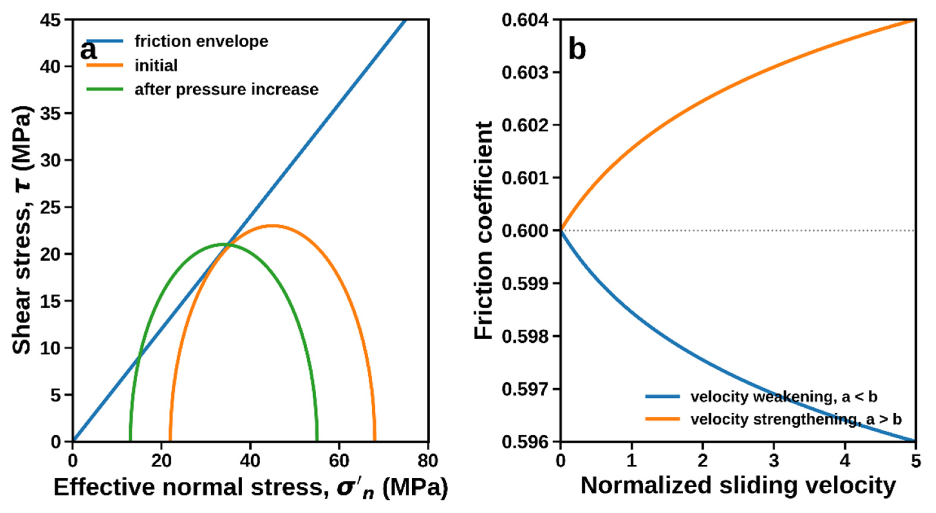
Figure 3a illustrates the leftward shift of a stress state in effective stress space as pressure increases. The figure is schematic: the actual stress path can involve simultaneous changes in circle center and radius because poroelastic and thermal stresses are not generally isotropic.
4.2. Poroelastic Stress Transfer and Pressure Diffusion
Quasi static mechanical equilibrium is
with constitutive behavior relating total stress to elastic or inelastic strain, pore pressure, and temperature. In linear isotropic thermo poroelasticity,
where and are Lamé parameters, is drained bulk modulus, and is the linear thermal expansion coefficient. The thermal term represents a fully constrained isotropic contribution within this constitutive form; thermal stress in a reservoir is determined by compatibility and boundary conditions. Unconstrained cooling produces strain but not stress.
Pressure propagation is often interpreted using hydraulic diffusivity. For a simplified single phase homogeneous medium,
where is permeability, is viscosity, is specific storage, and is a characteristic diffusion distance. This scaling is useful for estimating whether a fault can be pressurized during a given operation, but it can fail in multiphase flow, heterogeneous formations, and connected fracture networks. A permeable fault or high permeability corridor can transmit pressure much farther than the CO₂ saturation plume, while a sealing fault can compartmentalize pressure and increase local gradients [41,42,43].
Poroelastic stress transfer can affect faults outside the region of appreciable pressure change. Expansion of the pressurized reservoir changes shear and normal stress in adjacent formations and basement. The sign and magnitude of this transfer depend on reservoir geometry, mechanical layering, fault orientation, and boundary conditions. Consequently, a field interpretation should not infer pressure diffusion solely from event migration unless a coupled model and location uncertainties support that conclusion.
4.3. Multiphase Flow and Component Conservation
CO₂ storage requires component wise mass conservation because water and CO₂ may partition between aqueous and CO₂ rich phases. For component ,
where denotes phase, saturation, density, component mass fraction, Darcy flux, and diffusive flux. Darcy flux is
Closure requires capillary pressure and relative permeability relations, equations of state, phase equilibrium, and saturation constraints. These choices influence pressure near the plume and therefore fault loading. A single phase pressure model can be useful for conservative screening, but its bias is site and scenario dependent; it should be checked rather than assumed.
4.4. Thermal Effects
Injected CO₂ can be colder than the formation because of surface conditions, wellbore heat exchange, and expansion. Temperature influences density, viscosity, solubility, and phase behavior and can induce constrained thermal contraction near the well. The governing energy equation is most consistently written in terms of internal energy or enthalpy, including conductive and advective heat transport and, where relevant, phase change and Joule Thomson effects. A simplified form is
where is bulk internal energy density, phase enthalpy, and effective thermal conductivity.
Cooling may reduce horizontal compressive stress near an injection well, promote tensile fracture, alter fault normal stress, or create differential stress across mechanical interfaces. Whether it stabilizes or destabilizes a particular fault depends on orientation and constraints; “cooling causes tensile stress” is not a complete field statement. Thermal influence is strongest where temperature change is appreciable and may be secondary to pressure at distant faults. Fully coupled analysis is most important for cold injection, high rates, low permeability formations, strong thermal contrasts, and faults or caprock near the cooled volume [13,44,45,46].
4.5. Friction, Stability, and Nucleation
Mohr Coulomb friction defines an onset condition but not the stability of sliding. Rate and state friction represents friction coefficient as a function of slip velocity and a state variable :
with the aging law
Here describes the direct velocity effect, the state evolution effect, and a characteristic slip distance. At steady state, corresponds to velocity weakening and can permit unstable slip when elastic stiffness is sufficiently low; corresponds to velocity strengthening and generally favors stable sliding. Mineralogy, temperature, effective normal stress, surface roughness, gouge thickness, and fluid chemistry affect these parameters [47,48,49,50].
A characteristic nucleation size can be written schematically as
for velocity weakening conditions, where the dimensionless coefficient depends on geometry, loading stiffness, dimensionality, and the selected state evolution law. The expression is retained only as a scaling relationship: the numerical prefactor and, in some formulations, the characteristic form differ among spring slider, two dimensional, and three dimensional continuum models. It should therefore not be used with a universal coefficient or interpreted as a precise field threshold without a consistent frictional model and calibrated parameters [51,52].
Figure 3b contrasts velocity weakening and velocity strengthening steady state behavior. Laboratory parameters cannot be transferred directly to kilometer scale faults without considering scaling, heterogeneity, and the possibility that only part of the fault is velocity weakening.
Figure 3.
Fault stability and frictional response. (a) Schematic Mohr representation showing the reduction of effective normal stress as pressure increases. The friction envelope remains unchanged in this simplified illustration. (b) Schematic steady state rate and state friction showing velocity weakening when a is less than b and velocity strengthening when a is greater than b. Original synthesis based on Byerlee [53], Dieterich [47], Ruina [48], Marone [49], and Segall and Lu [41].
Figure 3.
Fault stability and frictional response. (a) Schematic Mohr representation showing the reduction of effective normal stress as pressure increases. The friction envelope remains unchanged in this simplified illustration. (b) Schematic steady state rate and state friction showing velocity weakening when a is less than b and velocity strengthening when a is greater than b. Original synthesis based on Byerlee [53], Dieterich [47], Ruina [48], Marone [49], and Segall and Lu [41].
4.6. Fault Hydraulic Behavior and Permeability Evolution
Faults are not uniformly conductive or sealing surfaces. A fault zone may contain a low permeability gouge core, permeable damage zones, relay structures, mineralized lenses, and intersections that control three dimensional connectivity. Slip can compact gouge, dilate asperities, create new fractures, or close existing pathways depending on effective stress and shear history. The hydraulic consequence of reactivation must therefore be modeled as an evolving structure rather than a binary “sealed/open” switch.
For ideal parallel plates separated by hydraulic aperture , laminar flow per unit width follows the cubic law,
The corresponding intrinsic permeability is . The distinction matters: transmissivity scales with , whereas intrinsic permeability scales with . Natural faults depart from the parallel plate ideal because roughness, contact area, tortuosity, channelization, multiphase occupancy, and gouge affect flow [54,55,56].
Mechanically coupled permeability laws should be selected according to evidence. Exponential effective stress relations may represent matrix or fracture closure over a calibrated range. Barton Bandis type relations can represent nonlinear normal closure. Shear dilation laws can relate aperture to plastic shear displacement. Damage models can link permeability to crack density. Each law introduces parameters that are often more uncertain than elastic properties, so sensitivity and uncertainty analysis are essential.
4.7. From Slip to Seismic Moment and Magnitude
Seismic moment is
where is seismic slip. Moment magnitude is commonly written
when is in N·m. A quasistatic model may calculate total fault displacement but cannot assume that all displacement is seismic. Stable sliding, distributed plasticity, fracture creation, and frictional heating can consume energy without equivalent radiation. A dynamic or explicitly calibrated seismic source model is required to estimate seismic moment consistently [32,57].
Empirical rupture scaling relations can bound plausible magnitude for mapped structures, but they carry large epistemic uncertainty and were largely derived from tectonic earthquakes. Maximum magnitude at an injection site depends on the connected, critically stressed portion of a fault and on rupture arrest conditions, not simply on injected volume or mapped fault length. For risk assessment, magnitude should therefore be represented probabilistically and conditioned on alternative fault geometries and stress states.
4.8. Structural Uncertainty, Fault Architecture, and Hydraulic Connectivity
Fault geometry is not merely a visualization input; it is a dominant part of the physical hypothesis. A fault interpreted from reflection seismic data may represent a single surface, a segmented system, or the envelope of a broader damage zone. Throw, tip line position, relay zones, branch faults, and intersections can control both pressure communication and rupture arrest. Seismic resolution generally decreases near steep or complex structures, while wells sample only a very small part of the fault system. A deterministic surface therefore understates epistemic uncertainty even when it is geometrically detailed.
A practical geomodel should distinguish the fault core, damage zone, and surrounding host rock when evidence supports that level of detail. The core may be clay rich and sealing across the fault while the damage zone is transmissive along strike. Alternatively, cementation can reduce damage zone permeability, or shear dilation can produce a transient conductive pathway. Juxtaposition of reservoir and caprock units creates direction dependent capillary and hydraulic behavior that cannot be represented by one scalar “fault permeability.” Mechanical stiffness and strength can also differ between the core, damage zone, and host rock. These distinctions explain why fault slip does not imply leakage and why a hydraulically conductive fault is not necessarily mechanically weak [11,34,56].
Connectivity uncertainty should be represented through ensembles of structural scenarios rather than a single smoothed interpretation. Scenarios may vary fault continuity, segmentation, transmissibility multipliers, damage zone width, relay connectivity, and connections to the injection interval, basement, or overburden. The ensemble should be conditioned to seismic interpretation, well intersections, pressure interference, tracer response, and deformation observations. Structural alternatives that are visually plausible but inconsistent with observed pressure or displacement should be down weighted; alternatives that remain observationally equivalent should be retained in the posterior uncertainty.
The consequences of an unresolved connection depend on the prediction target. For reservoir pressure, a connected conductive structure may provide pressure relief and reduce near well pressure. For fault stability, the same connection may transmit pressure to a larger critically stressed area. For containment, pressure relief within the reservoir may be beneficial while vertical migration along a connected damage zone may be unfavorable. A model should therefore avoid assigning “good” or “bad” labels to fault transmissivity without specifying the affected metric and time scale.
Structural uncertainty also interacts with numerical resolution. A fault represented as a zero thickness interface can reproduce traction and slip but may not reproduce storage, pressure gradients, or distributed deformation within a finite width zone. A volumetric fault zone model resolves those processes but adds parameters and mesh requirements. Embedded fracture and lower dimensional formulations provide an intermediate option. The representation should be selected by comparing characteristic fault zone width, grid size, pressure gradient scale, and required output not by software availability alone.
5. Multiphysics Numerical Modeling
5.1. Model Architecture and Coupling Choices
A storage geomechanics model is defined by more than its software name. At minimum, the formulation must specify conservation equations, primary variables, constitutive models, fault representation, coupling strategy, spatial discretization, temporal integration, nonlinear solution method, boundary conditions, initial stress, well controls, and the method used to translate fault response into risk metrics. Two models implemented in the same software can give different answers because they encode different physical hypotheses.
Three coupling architectures are common. In one-way sequential coupling, flow and heat are solved first and pressure and temperature are passed to a mechanical model. Mechanical deformation does not update flow properties. This architecture is efficient and can be adequate when deformation is small and permeability is insensitive to stress. It is unsuitable when slip, dilation, compaction, or fracture opening materially changes flow.
In two way staggered coupling, flow/heat and mechanics are solved alternately, and porosity, permeability, aperture, or stress dependent properties are exchanged until a convergence criterion is met. Fixed stress splitting is widely used because of its stability for poromechanical problems. Accuracy depends on time step size, transfer operators, and convergence tolerance. A single pass per time step is not equivalent to a converged two-way scheme [18,19,58,59].
In a monolithic formulation, hydraulic, thermal, mechanical, and possibly fault state variables are solved in one nonlinear system. Monolithic methods can be robust for strong coupling and avoid splitting error, but they demand effective preconditioners, consistent Jacobians, and substantial memory. Their theoretical coupling strength does not guarantee superior field prediction if constitutive parameters and geology are poorly constrained. Figure 4 summarizes the information flow and feedback represented by the three coupling architectures.
The appropriate architecture depends on the question. Regional pressure management may be dominated by multiphase flow and can use a simplified geomechanical response. Near fault slip prediction may require two way coupling because aperture and permeability evolve. Dynamic rupture is often separated from long term injection because the time scales differ by many orders of magnitude: a reservoir model may use hours to months, whereas rupture propagation requires subsecond resolution. A practical workflow can therefore couple a long term quasistatic model to a local dynamic model when a fault patch approaches a specified instability condition.
5.2. Continuum Finite Element Methods
The finite element method is well suited to complex geometry, material heterogeneity, contact interfaces, and unstructured meshes. Displacement based elements are standard for elasticity and plasticity, while mixed formulations are often needed to avoid pressure oscillations or volumetric locking in nearly incompressible poromechanics. Stable interpolation pairs, stabilization, or mixed finite elements should be documented, especially for low permeability formations and short time steps.
Faults can be represented in several ways. A conforming interface aligns the mesh with the fault and applies contact, cohesive, or interface elements. This approach provides direct control of normal and shear behavior and supports aperture dependent flow, but meshing becomes difficult for intersecting networks. A thin fault zone represents the fault as a finite thickness continuum with plasticity, damage, or anisotropic permeability. It can represent gouge and damage zone processes but introduces a thickness that may be numerical rather than geological. A nonconforming embedded or enriched interface avoids matching the mesh to the fault but requires special integration and stabilization.
Commercial finite element packages such as Abaqus and COMSOL are frequently used because they provide nonlinear mechanics, contact, thermal expansion, and user defined constitutive options. Their strengths include mature solvers and rapid model development. Limitations arise when multiphase compositional flow, equation of state behavior, and fracture network flow must be coupled in detail. User subroutines or external coupling may be required, and reproducibility can be limited when model files and scripts are not shared. Open frameworks such as MOOSE and OpenGeoSys offer source code access, parallelism, and extensibility, but require greater software development expertise [20,60].
Finite element accuracy should be demonstrated through spatial and temporal convergence for the quantities of interest, not simply global displacement. Fault traction and slip can be sensitive to mesh alignment and interface interpolation. A mesh that adequately resolves pressure may still be too coarse for stress concentration or nucleation. Conversely, resolving a diffuse fracture length scale everywhere can make field scale models impractical. Goal oriented refinement near faults and wells is preferable to uniform refinement when error indicators are available.
5.3. Finite Volume, Finite Difference, and Reservoir Geomechanics Coupling
Finite volume and integrated finite difference methods dominate reservoir simulation because they conserve mass locally and handle complex multiphase constitutive behavior. Structured finite differences are computationally efficient but less flexible for irregular faults and stratigraphy. Many storage studies therefore couple a flow simulator to a separate mechanical solver. TOUGH FLAC is a prominent example: TOUGH family simulators calculate multiphase mass and energy transport, and FLAC3D calculates deformation and stress. State variables are exchanged between grids or zones, with iterations when two-way coupling is required [17,61].
Reservoir to mechanics transfer requires care. Pressure and saturation may be cell centered on one grid, while stress and displacement are represented on another. Interpolation must preserve volume and avoid artificial smoothing near faults. Mechanical boundaries must be placed sufficiently far from the region of interest or assigned conditions that reproduce the regional stress response. Lateral pressure boundaries can strongly affect storage scale pressure buildup; closed boundaries may exaggerate pressure if the physical system is hydraulically open, whereas fixed pressure boundaries may understate interference if their placement is unrealistic.
Explicit finite difference geomechanics, as used in FLAC3D, avoids assembly of a global stiffness matrix and handles large deformation and nonlinear constitutive behavior. Quasi static equilibrium is obtained by dynamic relaxation. The explicit stability limit can require small mechanical time steps, but reservoir time can be advanced in larger increments through coupling logic. Dynamic rupture can also be represented, although seismic wave simulation and long term multiphase flow are usually separated because their stable time steps differ drastically.
5.4. Discrete Element and Finite Discrete Element Methods
Discrete element methods represent rock as interacting blocks or particles and are attractive where discontinuities dominate response. Block based methods can represent mapped fault surfaces, intersections, opening, rotation, and large shear displacement. Particle based and bonded block methods can simulate fracture nucleation, coalescence, grain scale damage, and shear localization. Fluid flow may be solved through contact networks or coupled continuum domains [62,63,64].
The primary advantage is explicit kinematics. Fault opening and slip need not be inferred from a smeared plastic strain. The primary limitation is calibration. Contact normal and shear stiffness, bond strengths, friction, dilation, damping, particle size, and fracture flow parameters are not all directly measurable at field scale. Multiple microparameter combinations may reproduce the same elastic modulus and peak strength but predict different post peak behavior. Calibration should therefore include stress and strain response, dilation, permeability evolution, and fracture patterns, with independent validation where possible.
Discrete fracture network models occupy a related but distinct category. A DFN represents statistical or mapped fracture geometry and may be coupled to continuum deformation. It is valuable for evaluating connectivity, pressure channeling, and the effect of fault intersections. Uncertainty in fracture intensity, size distribution, orientation, termination, and hydraulic aperture can dominate the predicted pressure path. Ensemble analysis is therefore more informative than one “best” realization [56].
Finite discrete element methods combine deformable continuum elements with explicit fracture creation and contact after separation. They can represent transition from intact rock damage to block motion, but field scale THM applications are computationally demanding. Their greatest value may be in laboratory scale process studies and in generating constitutive understanding for larger scale models.
5.5. XFEM, Embedded Discontinuities, and Phase Field Fracture
The extended finite element method enriches approximation spaces so that displacement jumps and crack tip fields can be represented without conforming the mesh to a crack. It is effective for crack growth and interaction with complex geometry. Coupled flow requires additional enrichment for pressure discontinuities or fracture flux, and frictional contact after crack formation is more difficult than tensile opening [65,66,67].
Embedded discontinuity and cut cell methods pursue similar goals: faults intersect the background mesh, and special interface terms enforce traction and flow conditions. These approaches can represent large networks without remeshing, but numerical conditioning, small cut cells, and accurate transfer of fault aperture remain active research topics.
Phase field fracture represents a crack as a diffuse damage zone governed by an energy functional. It naturally handles nucleation, branching, and coalescence without explicit topology tracking. The regularization length controls the diffuse crack width and must be resolved by multiple elements, with adequacy demonstrated through mesh and length scale convergence. Phase field models are mature for brittle tensile fracture but more difficult for frictional shear, contact after fracture, and multiphase flow along a sharp discontinuity. Field application is limited by the fine mesh needed near fractures and by uncertainty in relating the numerical regularization length to a physical process zone size.
5.6. Analytical and Semi Analytical Models
Analytical models remain essential. They provide transparent pressure and stress scaling, rapid screening, and verification benchmarks. Line source or radial flow solutions estimate pressure diffusion. Poroelastic inclusion and nucleus of strain solutions estimate deformation. Slip tendency and critically stressed fault calculations rank structures. Rate and state spring slider models clarify stability. Their value is greatest when assumptions are explicitly compared with the site and when they are used to bracket or verify numerical results rather than presented as high fidelity forecasts.
A hierarchical workflow can begin with analytical screening, proceed to a regional flow model, couple selected scenarios to geomechanics, and use local discontinuum or dynamic models only for the faults that control risk. This is more efficient and auditable than building a highly detailed monolithic model before the dominant uncertainties are understood.
5.7. Capability Comparison
Figure 5 compares modeling families using an author defined capability rubric rather than a vendor ranking. The scores use the evidence coding in Table 1: 0 indicates that the capability is not intrinsic to the formulation; 1 indicates that it is possible only with substantial extension or is supported by limited demonstrations; 2 indicates repeated demonstration with material limitations; and 3 indicates a comparatively mature or widely demonstrated capability for the stated use. The matrix summarizes typical strengths, not the performance of every implementation, and should be read together with the limitations in Table 3.
5.8. Constitutive Models for Intact Rock and Faults
Linear elasticity is suitable when stresses remain well below yield and deformation is small. Mohr Coulomb and Drucker Prager plasticity are common for intact rock and fault zones. Mohr Coulomb represents pressure dependent shear strength with distinct friction and cohesion; Drucker Prager provides a smooth approximation convenient for numerical solution but must be matched carefully in compression and extension. Cap plasticity is useful for compaction and pore collapse in weak formations. Damage mechanics represents progressive stiffness loss and can be coupled to permeability. Viscoelastic or viscoplastic behavior may matter in evaporites, shales, and long after injection periods.
For preexisting faults, constant friction contact is the simplest model. It can calculate the onset and amount of quasistatic slip under imposed loading but lacks healing and velocity effects. Slip weakening laws reduce friction over a characteristic distance and are common in dynamic rupture. Rate and state friction represents velocity and state dependence and can generate delayed or accelerating slip. Elastoplastic fault zone models distribute strain over finite thickness and can include dilation and hardening/softening. Cohesive laws are appropriate for bonded interfaces or new fracture but should not be used as a substitute for friction once surfaces are in contact. Table 4 links each constitutive choice to the response it represents, the questions it can support, and the conclusions that require additional model components.
5.9. Initial and Boundary Conditions
Initial stress is often the largest source of uncertainty. A model should document vertical stress, minimum and maximum horizontal stress, orientations, pore pressure, stress gradients, and the evidence supporting them. Leak off tests, extended leak off tests, mini fracture tests, borehole breakouts, drilling induced tensile fractures, image logs, focal mechanisms, density logs, and regional stress databases constrain different parts of the stress tensor and have different uncertainties. A deterministic “best” stress state can hide the possibility that a plausible alternative places a fault much closer to failure.
Initial pore pressure and temperature must be consistent with depth, salinity, and formation connectivity. Depleted reservoirs require a history matched production state because depletion changes stress and may produce irreversible compaction. Fault pressure should not automatically equal reservoir pressure when fault core transmissibility is uncertain.
Mechanical boundaries can create artificial stress changes if placed too close. Roller boundaries constrain normal displacement and may not reproduce regional compliance. Prescribed far field stress boundaries can be preferable but require consistent traction. Hydraulic boundaries should reflect connected aquifers, pressure management wells, and the scale of pressure interference. Sensitivity to boundary placement should be reported for field scale studies.
5.10. Verification, Convergence, and Numerical Credibility
Verification asks whether the equations are solved correctly. Relevant tests include mass and energy balance, patch tests, manufactured solutions, Terzaghi consolidation, the Mandel Cryer effect, thermal consolidation, two phase flow benchmarks, contact tests, and frictional sliding benchmarks. Mesh and time step convergence should be evaluated for the actual risk quantity: critical pressure, slip, aperture, maximum ΔCFS, or leakage rate. Solver tolerance should be tight enough that numerical error is small relative to parameter uncertainty.
Coupled models should report conservation residuals and the convergence of staggered iterations. Artificial damping, penalty factors, contact regularization, and stabilization parameters can influence slip and must be sensitivity tested. A converged nonlinear solver does not prove physical correctness; it only indicates consistency with the discretized equations.
6. Thermal Hydraulic Mechanical and Chemical Feedbacks
6.1. Pressure, Saturation, and Stress Paths
The stress path during injection is controlled by more than the direct effective stress term. In a laterally extensive reservoir, expansion can increase horizontal total stress while vertical total stress may remain approximately controlled by overburden. The result depends on Poisson’s ratio, layer stiffness, reservoir geometry, lateral confinement, and hydraulic boundaries. An expression that subtracts the same from all three principal total stresses is therefore not generally valid. Effective stress trajectories should be calculated from a consistent poroelastic boundary value problem.
Multiphase saturation affects mobility and pressure distribution. Near the well, CO₂ relative permeability, brine relative permeability, and capillary pressure control injectivity. Away from the plume, pressure may propagate through brine with little CO₂ saturation. Dissolution changes CO₂ mass distribution but usually evolves more slowly than pressure during active injection. Fault risk is therefore often governed by the pressure footprint rather than the saturation plume, although fault transmissibility and capillary entry pressure determine whether CO₂ can enter a fault.
6.2. Mechanical Feedback on Flow
Pore volume change can be represented through porosity updates derived from volumetric strain and grain compressibility. Permeability may be coupled to porosity through empirical relations, but these relations should be calibrated for the relevant rock and stress path. Matrix permeability can decrease during compaction and increase during unloading or damage. Fracture transmissivity can change much more strongly because of aperture sensitivity.
Fault reactivation can create competing feedbacks. Dilation increases transmissivity and may dissipate pressure along the fault, potentially reducing local effective stress change while transmitting pressure to a larger area. Gouge mobilization or shear compaction may reduce transmissivity and localize pressure. New fractures can connect previously separated compartments. Whether feedback is stabilizing or destabilizing is therefore scenario specific.
A robust coupled analysis should track pressure work, mechanical work, plastic dissipation, and mass balance. If a fault permeability jump is imposed at a slip threshold, the magnitude and persistence of the jump should be justified and sensitivity tested. Instantaneous orders of magnitude changes are sometimes used to explore bounding behavior, but they should not be presented as calibrated predictions without evidence.
6.3. Thermal Mechanical Interaction
Cold CO₂ injection can produce a thermal front smaller than the pressure footprint because thermal diffusivity and advective heat transport differ from hydraulic pressure propagation. Near the well, constrained contraction can reduce horizontal stress, alter fracture pressure, and promote tensile damage. At a dipping fault, the resolved change in normal and shear traction depends on fault orientation relative to the cooled volume. Thermal effects can also alter friction and chemical reaction rates.
A useful modeling hierarchy is to begin with a nonisothermal reservoir model to establish the magnitude and extent of cooling, then compare isothermal and thermal mechanical simulations for the same pressure field. If the change in fault traction is small relative to stress uncertainty, a simpler model may be defensible for regional screening. If the fault intersects the cooled region or the injection temperature contrast is large, fully coupled analysis is warranted [13,44,46].
6.4. Geochemical and Chemo Mechanical Effects
CO₂ dissolution lowers brine pH and can drive mineral dissolution and precipitation. These reactions alter porosity and permeability and may affect fault gouge, cement, and caprock. Carbonate dissolution can increase local porosity, whereas secondary precipitation can reduce pore space or seal pathways. Clay reactions and changes in surface chemistry may influence friction, swelling, and fines migration. Reaction induced changes are often slow relative to pressure buildup but can matter over years to centuries and near reactive mineral surfaces.
Fully coupled THMC models remain uncommon because constitutive links between reaction progress and mechanical properties are poorly constrained. A sequential workflow is often more defensible: reactive transport predicts mineral volume change; laboratory data or calibrated relations map mineral change to elastic, strength, or permeability properties; geomechanics updates stress and deformation. The uncertainty introduced by each mapping should be reported. Taron et al. [69] provide a general framework for coupled thermal, hydraulic, mechanical, and chemical processes, but storage specific validation of fault friction under CO₂ rich brine remains limited.
6.5. Dimensionless Analysis and Model Reduction
Dimensionless groups help determine which processes require explicit representation. A hydraulic diffusion ratio compares domain scale with pressure diffusion length. A thermal analogue uses thermal diffusivity. A Péclet number compares advective and conductive heat transport. Capillary number compares viscous and capillary forces. Damköhler numbers compare reaction and transport time scales. These quantities are meaningful only when their characteristic length and time scales are defined.
Any proposed coupling metric should be dimensionless and should state the characteristic length, storage, stress, temperature, and time scales used in nondimensionalization. Dimensional consistency is a necessary first check, followed by sensitivity testing to show that the metric discriminates regimes relevant to the selected prediction target. This prevents a convenient algebraic ratio from being interpreted as a transferable physical threshold.
Reduced order modeling should preserve the mechanisms relevant to the target. A pressure surrogate may not need to reproduce every saturation detail if its purpose is fault loading, but it must preserve pressure gradients and boundary effects. A slip surrogate must preserve threshold behavior and should be trained densely near the failure boundary. Model reduction is therefore goal oriented rather than purely based on global variance.
7. Laboratory and Field Evidence
7.1. Why Validation Must Be Hierarchical
A model can be numerically verified and still be physically wrong. Constitutive validation requires experiments in which material properties and boundary conditions are measured. Field validation is harder because the stress field, fault geometry, and monitoring coverage are uncertain. The most credible workflow therefore combines canonical benchmarks, laboratory tests, and field observations, with each level testing different assumptions.
Laboratory experiments are especially valuable for distinguishing onset from post onset behavior. Direct shear, triaxial, and true triaxial tests on saw cut or natural faults can measure friction, dilation, permeability, slip velocity, and acoustic emissions while pore pressure is controlled. Tests with brine and CO₂ rich fluids can examine chemical and phase effects. However, scaling from centimeters to kilometers is nontrivial: laboratory faults are smoother or more uniform, normal stress is lower, loading stiffness differs, and the available rupture area is constrained.
7.2. Core Scale and Fault Slip Experiments
A complete laboratory validation dataset should report specimen geometry and orientation, mineralogy, porosity, permeability, saturation protocol, fluid composition, temperature, confining and axial stresses, pore pressure locations, displacement measurement, loading system stiffness, fault roughness, and acoustic sensor geometry. Raw or minimally processed pressure, displacement, and acoustic data should be archived when possible.
For static or quasistatic models, the primary validation targets are critical pore pressure, shear displacement, dilation, normal displacement, and permeability evolution. For rate and state models, velocity step and slide, hold, and slide tests constrain , , , and healing. For dynamic models, source spectra, stress drop, rupture velocity, and radiated energy are relevant. Fitting peak strength alone is insufficient because multiple constitutive laws can reproduce peak stress while predicting very different slip and permeability.
Acoustic emission provides a high resolution indicator of distributed damage and fault slip. Event counts are strongly affected by threshold and sensor coupling, so absolute rates are not transferable without calibration. Waveform clustering and focal mechanism proxies can distinguish tensile and shear dominated processes, but labels themselves carry uncertainty. Continuous acoustic features can contain state information even when discrete event catalogs are incomplete [21,70,71,72].
7.3. In Salah
The In Salah project in Algeria is a central case for storage geomechanics because injection produced measurable surface deformation and a microseismic response. InSAR revealed uplift patterns, including a double lobed feature near injection well KB 502 that motivated models involving opening or deformation of a deep fracture zone. Coupled reservoir geomechanical studies showed that pressure, mechanical layering, and fault or fracture representation can reproduce important aspects of the deformation pattern [73,74,75,76].
The seismic evidence must be interpreted with its limitations. Stork et al. [77] detected 9,506 events using data that relied largely on a single three component geophone, but only a selected subset could be located with useful confidence. This limits precise claims about spatial clustering and model location error. The case demonstrates the value of integrating deformation, pressure, and seismic evidence, and also the danger of assigning high spatial precision to an underdetermined monitoring geometry.
In Salah does not support a universal conclusion that thermal effects are either dominant or negligible. The relative contribution depends on injection temperature, model assumptions, and the region of interest. The stronger lesson is that surface deformation can reveal subsurface structures not represented in an initial geomodel and can materially change the geomechanical interpretation.
7.4. Illinois Basin Decatur
The Illinois Basin Decatur Project injected approximately one million tonnes of CO₂ into the Mt. Simon Sandstone and recorded a large microseismic catalog. Events occurred primarily below the reservoir in the Precambrian basement and were small, but the dataset provides rare evidence for evaluating hydromechanical triggering during CO₂ storage [78].
Luu et al. [79] modeled the sequence using coupled hydromechanics and a statistical earthquake model. The study illustrates how pressure diffusion and poroelastic stress changes can be integrated with a fault population and seismicity formulation. It also demonstrates the uncertainties that remain: basement permeability, fault distribution, background stressing, magnitude completeness, and source locations. The project should not be summarized by unsupported single values for “location RMSE” or “magnitude bias” unless those values are explicitly reported by a specific validation study.
The Decatur evidence emphasizes that the storage reservoir, caprock, and basement form a mechanically coupled system. Describing stress as transmitted “through the caprock to the basement” is geometrically misleading because the caprock overlies the reservoir while the basement lies below it. The relevant mechanisms are pressure communication, reservoir expansion, mechanical layering, and stress transfer into underlying crystalline rock.
7.5. Otway
The Otway International Test Centre has hosted a sequence of controlled storage and monitoring experiments. Its value lies in well characterized injection, extensive active and passive seismic monitoring, fiber optic measurements, and experiments designed to test detection and plume monitoring methods [80]. A Stage 2C injection of a comparatively small CO₂ rich volume was associated with microseismicity interpreted as activation of a previously unresolved small fault in a permeable saline aquifer [81].
This case is important because it shows that detectable seismicity can occur without large overpressure when buoyancy and local connectivity transmit pressure to a susceptible structure. It also highlights the distinction between “no damaging seismicity” and “no seismic response.” Monitoring sensitivity and the definition of the target determine what is observed. Otway is therefore useful for evaluating detection, fault characterization, and model updating rather than for claiming a universal negative prediction.
7.6. Additional Storage Context: Sleipner, Snøhvit, and Ketzin
Long running storage projects that were not designed as fault reactivation experiments still provide important contextual evidence. At Sleipner, repeated seismic and gravimetric surveys demonstrate long term plume conformance monitoring at industrial scale, but the site offers little direct validation of fault slip or dynamic rupture models [82]. At Snøhvit, rapid pressure increase, near well injectivity impairment, fault segment connectivity, and transfer to a fallback injection interval illustrate how pressure limits and geological compartmentalization can control operational decisions [83].
At Ketzin, integrated pressure, seismic, electrical, geochemical, and modeling workflows supported a research scale injection and after injection program [84]. These sites strengthen the evidence for monitoring design, history matching, pressure management, and model updating. They do not constitute prospective validation of seismic rupture forecasts and are therefore treated as contextual storage evidence rather than direct fault reactivation benchmarks.
7.7. Basel and Other Injection Analogues
The 2006 Basel enhanced geothermal stimulation induced an event of approximately magnitude 3.4 and led to project termination. Although water injection into crystalline basement differs from CO₂ storage in sedimentary formations, Basel provides transferable lessons about critically stressed faults, event rate response to injection, after injection seismicity, magnitude uncertainty, and traffic light design [85,86].
Wastewater disposal and hydraulic stimulation analogues further demonstrate that pressure can migrate through connected formations and that large events may occur on faults not fully characterized before injection. These analogues should inform conservative fault screening, monitoring, and pressure management. They should not be pooled directly with storage projects to estimate a single event probability because injection rates, fluid properties, geology, pressure history, and monitoring completeness differ.
7.8. What Field Cases Can and Cannot Validate
Pressure history is usually the strongest field constraint because injection and observation wells provide direct measurements. Surface or borehole deformation provides spatial information about reservoir pressurization and mechanical structure. Microseismic catalogs provide timing and approximate source locations but are conditioned by network geometry, velocity model, detection threshold, and processing. Independent geomechanical models are available for several sites, but prospective risk forecasts remain rare.
Figure 6 summarizes evidence availability for four cases selected because they provide direct geomechanical or induced seismicity lessons. “Strong” denotes multiple independent data types together with peer reviewed model evaluation; “moderate” denotes useful but incomplete spatial, temporal, or methodological coverage; and “limited” denotes sparse observations, restricted monitoring geometry, or absence of prospective testing. The categories describe the suitability of evidence for model evaluation, not project safety. The broader storage context in Section 7.6 is included in Table 5 but not scored in Figure 6 because those projects were not designed primarily as fault reactivation benchmarks.
7.9. Recommended Validation Reporting
Every model data comparison should identify which observations were used for calibration and which were held out. The observation operator the mapping from model state to measurement must be described. For example, InSAR measures line of sight surface displacement, not reservoir strain directly. A seismic catalog is filtered by detection and location procedures. Pressure gauges may record wellbore effects rather than formation pressure during transient injection.
Uncertainty should be propagated into the comparison. A predicted hypocenter should be compared with an observed location probability volume, not a single point. Magnitude predictions should specify magnitude scale and uncertainty. Deformation comparison should include atmospheric and orbital corrections where relevant. Visual agreement alone is insufficient when quantitative data are available.
7.10. Transferable Lessons from Geothermal and Other Injection Analogues
Enhanced geothermal systems, wastewater disposal, gas storage, and hydrocarbon production provide much larger induced seismicity datasets than CO₂ storage. These analogues are valuable because they expose processes that may be difficult to observe during a storage pilot: rapid pressure transmission along faults, aseismic slip preceding seismic rupture, delayed post shut in events, interaction among multiple faults, and the operational consequences of an event larger than anticipated. Basel demonstrates that maximum magnitude cannot be inferred reliably from injected volume or small event behavior alone, and that after injection seismicity must be considered in shutdown protocols [85,86]. Laboratory and field studies outside CO₂ storage also show that poroelastic stress transfer and aseismic slip can trigger events beyond the most strongly pressurized zone [41].
Transfer must nevertheless be mechanistic rather than superficial. Water injection into crystalline basement differs from supercritical CO₂ injection into a sedimentary reservoir in fluid compressibility, viscosity, multiphase behavior, thermal contrast, fault mineralogy, matrix storage, and operational duration. Wastewater disposal commonly involves large regional well populations and long lived pressure interference; a storage project may have fewer wells but requires verified containment and may include pressure management wells. Geothermal stimulation intentionally enhances fracture transmissivity, whereas a storage project normally seeks to remain below conditions that create uncontrolled fractures. These differences mean that event rate coefficients, traffic light thresholds, and magnitude distributions should not be imported unchanged.
Three types of transfer are defensible. First, process transfer uses an analogue to establish a mechanism, such as rate and state nucleation, pressure diffusion, or after injection triggering. Second, method transfer adapts monitoring, catalog construction, probabilistic forecasting, or traffic light design while recalibrating site specific parameters. Third, prior transfer uses analogue data to define broad prior distributions, followed by updating with storage site data. Direct performance transfer claiming that a model accurate at a geothermal site will have the same error at a CO₂ site is generally not defensible.
Analogue selection should therefore be documented using a similarity matrix. Relevant dimensions include stress regime, fault lithology and maturity, reservoir depth, permeability structure, fluid phase and viscosity, temperature contrast, injection rate, cumulative volume, monitoring geometry, and magnitude of completeness. An analogue can be highly informative for one dimension and poor for another. Basel, for example, is highly informative for operational response and after injection behavior but less representative of multiphase plume physics. Otway and Decatur are more directly representative of storage monitoring, but their injection scales and structural settings do not cover all commercial projects.
A useful research strategy is to develop hierarchical models in which shared physical parameters are learned across analogues while site specific parameters remain distinct. Such models can borrow statistical strength without assuming geological identity. Their validation must hold out entire sites, not random time windows, and should report how predictions change as local data accumulate. This approach offers a more defensible path to multi-site learning than pooling all events into one undifferentiated dataset.
8. Machine Learning for Monitoring, Inference, and Forecasting
8.1. Separate the Task Before Selecting the Algorithm
Machine learning is most useful when the target, data generating process, and deployment environment are specified before an architecture is selected. At least four task classes should be separated: signal detection and phase picking; waveform or source classification; regression or inverse estimation of physical variables; and prospective forecasting of future fault or seismic response. A fifth class, surrogate modeling, approximates a simulator rather than observations. These tasks have different labels, sampling units, loss functions, validation designs, and levels of direct CO₂ storage evidence.
Signal detection identifies candidate events in continuous data. Phase picking estimates arrival times. Classification assigns an event to a class such as noise, blast, tensile crack, or shear dominated source. These tasks improve catalog completeness and reduce manual processing, but they operate after or during signal arrival. They do not by themselves forecast a future rupture. Prospective forecasting instead predicts event probability, event rate, magnitude distribution, or fault state over a future time window using only information available at the forecast issue time.
Figure 7a organizes inputs, model families, tasks, and outputs. Figure 7b shows the validation sequence needed to avoid data leakage. Training and test sets should be separated by physical unit event, specimen, experiment, time block, and preferably field site rather than by randomly shuffling highly correlated waveform windows.
Table 6 distinguishes evidence from direct CO₂ storage applications from evidence transferred from natural seismicity, laboratory friction, geothermal stimulation, and synthetic simulations. Maturity is assigned according to task directness, external validation, and prospective testing rather than model complexity.
8.2. Monitoring Analytics
Convolutional neural networks and transformer models have substantially improved earthquake detection and phase picking in large seismic datasets. Models such as generalized phase detectors and Earthquake Transformer learn waveform representations and can process continuous records rapidly [24,87,88]. For storage projects, these methods can lower detection thresholds, standardize processing, and support near real time catalog construction.
Deployment requires site specific checks. A model trained on tectonic earthquakes may be exposed to different frequency content, source and receiver geometry, instrumentation, and noise at a storage site. Borehole sensors and distributed acoustic sensing have directional responses that differ from conventional three component stations. Fine tuning can improve performance, but test events should be independent of training events and should include realistic noise. Detection performance should be reported as a function of signal to noise ratio and magnitude, not only as one aggregate accuracy.
Precision recall curves are generally more informative than receiver operating characteristic curves when events are rare. A low false positive rate can still produce an impractical number of false alerts when millions of windows are processed. Operational reporting should therefore include false detections per unit time, missed event rate above a stated magnitude or amplitude, latency, and changes in completeness relative to the baseline processing workflow.
Waveform classification can help distinguish mechanical processes in laboratory data. CNNs applied to spectrograms, one dimensional convolutions applied to raw traces, and recurrent or transformer models applied to sequences can identify reproducible signal patterns. However, laboratory labels such as “tensile” and “shear” are often inferred from simplified waveform ratios or source inversion and are not error free. A model cannot be more reliable than the label definition. Confusion matrices and class conditional uncertainty are therefore essential.
8.3. Feature Based Models for Fault Stability
Tree ensembles, support vector machines, generalized linear models, and Gaussian processes can predict slip indicators from injection, geological, and modeled features. Their main advantage is that they can combine nonlinear interactions and mixed data types while remaining relatively inexpensive. Physically meaningful inputs may include pressure change, pressure rate, distance and hydraulic connectivity to a fault, resolved normal and shear stress, slip tendency, fault orientation relative to the stress field, cumulative injection, temperature change, and recent seismicity.
Feature engineering can improve data efficiency, but it must not leak target information. A “Coulomb stress change” feature calculated using a model calibrated to the same events used for testing can make performance appear better than it is. Similarly, using cumulative event count up to the end of a forecast window is invalid. Every feature must be computable at the forecast issue time for a genuine prospective model.
Random forests and gradient boosted trees provide feature importance, but impurity based importance is biased toward continuous or high cardinality variables. Correlated features can split importance and obscure interpretation. Permutation importance and SHAP values are useful diagnostics, yet they explain the behavior of the fitted model rather than establish causation. A physically plausible importance ranking is encouraging, not proof that the model has learned the correct mechanism.
Gaussian process models are attractive for small datasets because they provide a predictive distribution and encode smoothness through kernels. Their cubic scaling with training size can be mitigated by sparse approximations. Bayesian generalized linear models provide transparent coefficients and uncertainty. These simpler models should be included as baselines; a deep network is not justified when a calibrated logistic or point process model performs similarly.
8.4. Time Series and Point Process Forecasting
Seismicity is an event process, not a conventional evenly sampled regression target. Event rate forecasting can use point process models, generalized linear models with count likelihoods, hidden state models, recurrent networks, or transformers. Poisson likelihoods are a starting point, but overdispersion and clustering may require negative binomial or self-exciting processes. ETAS type models capture event to event triggering but can confound injection forcing with aftershock interactions unless the components are separated [89].
Rate and state seismicity formulations provide a physics based link between stressing history and event rate. They can be driven by stress changes from a hydromechanical model and calibrated to a catalog. This approach preserves a mechanistic interpretation but inherits uncertainty in the stress calculation and the assumed fault population. Forecast evaluation should compare against simple baselines, including persistence, background rate, injection rate models, and standard point process models.
Sequence models such as LSTMs and transformers can integrate pressure, rate, temperature, deformation, and seismic history. They are flexible but susceptible to temporal leakage and nonstationarity. Random cross validation is inappropriate. A rolling origin or blocked evaluation should train on earlier intervals and test on later intervals. To evaluate spatial transfer, entire wells or sites should be held out. Performance may degrade after operational changes, sensor replacements, or changes in processing, so drift detection and periodic recalibration are needed.
Mean absolute percentage error is problematic for event counts because it is undefined or unstable near zero. Better metrics include Poisson or negative binomial deviance, continuous ranked probability score, log score, Brier score for event occurrence, calibration plots, and information gain relative to a baseline. For threshold based decisions, recall at a specified false alarm rate and lead time dependent precision are operationally interpretable.
8.5. Laboratory “Earthquake Prediction” and Scale Transfer
Laboratory friction experiments have shown that continuous acoustic features can track the evolving state of a sheared fault and estimate time to failure within a repeated experimental cycle [21]. These studies are scientifically important because they demonstrate that apparently noisy signals contain information about frictional state. They should not be described as direct field earthquake prediction. Laboratory apparatuses have controlled geometry, repeated loading, dense sensors, and a limited set of failure modes. Field faults are heterogeneous, incompletely observed, and subject to nonstationary loading.
Transfer can nevertheless be pursued mechanistically. Rather than transferring raw frequency features, models can target nondimensional or physically interpretable quantities such as normalized stress drop, acoustic energy rate, elastic modulus change, or state variable proxies. Domain adaptation can account for different sensor responses. Multiscale experiments can test whether features persist across sample sizes, roughness, confining stress, saturation, and fluid type. A field model should be validated prospectively before laboratory performance is used to support operational claims.
8.6. Class Imbalance, Calibration, and Uncertainty
Fault slip events and operationally significant seismicity are rare relative to normal operation. Overall accuracy is therefore misleading. A classifier that always predicts “no event” can have high accuracy while providing no value. Precision, recall, precision recall area, false alarm rate, and class specific calibration should be reported. Cost sensitive learning can reflect the asymmetric consequences of missed events and false shutdowns, but costs should be defined with operators and regulators rather than chosen only to optimize a score.
Probability calibration is essential. Reliability diagrams compare predicted probabilities with observed frequencies. Brier score and log loss assess probabilistic accuracy. Temperature scaling, isotonic regression, or Bayesian models may improve calibration, but calibration data must be independent. Uncertainty has at least two components: aleatoric uncertainty from noise and irreducible variability, and epistemic uncertainty from limited knowledge and distribution shift. Deep ensembles can approximate epistemic uncertainty but may remain overconfident outside the training domain.
Out of distribution detection should be part of deployment. Inputs can move outside the range of training pressure, temperature, geology, or sensor noise. The model should then abstain or widen uncertainty rather than issue a confident forecast. A human supervised system needs clear rules for when machine learning output is considered valid.
8.7. External and Cross Site Validation
The strongest test of generalization is a held out site. Within site random splits often place adjacent waveform windows, repeated cycles, or samples from the same experiment in both training and test sets. This measures interpolation within a known data generating process. It does not measure performance at a new storage project.
Cross site validation can be organized hierarchically. First, hold out entire events. Second, hold out specimens or experimental runs. Third, hold out time blocks that include operational changes. Fourth, hold out wells or monitoring arrays. Fifth, train on one or more sites and evaluate on a different geological site. Performance should be reported at each level because degradation reveals which variability the model fails to represent.
Federated learning may eventually enable multi-site training without sharing raw proprietary data, but heterogeneous labels, instruments, sampling rates, and geological regimes remain challenges. Privacy preserving aggregation does not solve domain shift. Common data schemas, benchmark tasks, and reference processing pipelines are prerequisites.
Table 7 summarizes the correct separation unit, preferred evaluation metrics, and common validation failure for each machine learning task.
8.8. Explainability and Causal Caution
Explainable AI methods can support model diagnosis. SHAP values can show how pressure, slip tendency, distance, or seismic history influence a prediction. Saliency or attention maps can identify waveform segments used by a detector. Counterfactual analysis can estimate how much an operational variable would need to change to alter a forecast. These tools are most useful when checked against known physics and when unstable explanations are reported.
Explanations are not causal evidence. Injection rate may appear important because it covaries with pressure, project phase, or monitoring quality. A model trained on historical operations cannot automatically predict the consequence of an intervention outside that history. Causal or decision focused analysis requires explicit assumptions, mechanistic constraints, or randomized/controlled variation that is rarely available in field operations. Physics based simulation can help evaluate interventions, while data driven models can update uncertain states; combining the two is generally more defensible than treating feature importance as a control law.
9. Physics Informed and Hybrid Scientific Machine Learning
9.1. What “Physics Informed” Should Mean
The term physics informed is used for several distinct strategies. A model may include physics derived input features, enforce conservation through the loss function, embed a differentiable simulator, learn a correction to a mechanistic model, or approximate a solution operator across parameterized PDE problems. These approaches have different guarantees. Using pressure or slip tendency as an input is physics guided feature engineering; it is not a physics informed neural network in the original PDE residual sense.
Three model classes are separated in this review. Physics constrained learners, including PINNs, enforce governing equation or interface residuals during training. Learned solution operators, including FNO, DeepONet, and graph operators, approximate mappings between input and solution fields across problem families. Simulator emulators and reduced order models, including POD, Gaussian processes, and CNN/RNN surrogates, approximate selected outputs of a specified full order model. Physics guided features and learned discrepancy corrections are cross cutting hybrid strategies rather than synonyms for PINNs.
Physics informed models are valuable when data are sparse but governing equations are trusted, when an inverse problem requires simultaneous state and parameter estimation, or when a fast differentiable approximation is needed. They are less attractive when the equations are misspecified, discontinuities dominate, or a conventional solver is already fast and reliable. The central question is not whether physics is present, but which physics is enforced, at what fidelity, and how residual satisfaction is verified.
9.2. Physics Informed Neural Networks
A PINN represents a state variable with a neural network and minimizes a loss containing observations, boundary and initial conditions, and residuals of governing equations. For coupled poromechanics,
Automatic differentiation evaluates derivatives of the network output. The weights control competition among residuals. Poor scaling can cause one equation to dominate training, so nondimensionalization, adaptive weighting, curriculum strategies, and domain decomposition are often necessary [14,26,28,90].
PINNs are sometimes called mesh free, but they still require discrete collocation, boundary, initial condition, and observation points. Their cost is shifted from linear/nonlinear solves to optimization. They do not automatically outperform finite elements. For smooth low dimensional benchmark problems, they can recover pressure and displacement and solve inverse problems with sparse sensors. For three dimensional heterogeneous multiphase fault problems, training can be more expensive and less robust than a conventional solver.
Faults create difficult discontinuities. Pressure, displacement, traction, and flux may be discontinuous or have sharp gradients across an interface. A single smooth network tends to smear these features. Domain decomposed PINNs, interface networks, mixture of experts’ architectures, level set representations, or hybrid finite element/PINN methods are more appropriate. Interface conditions, traction equilibrium, contact, friction, and flux continuity or jump, must be enforced explicitly.
9.3. Neural Operators
Neural operators learn mappings between functions, for example from permeability, boundary conditions, and well controls to pressure and displacement fields. Fourier neural operators, DeepONet, graph neural operators, and U shaped operator networks can evaluate new scenarios rapidly after training. They are promising for ensemble forecasting and uncertainty quantification because one trained model can approximate a family of PDE solutions [91,92,93].
Operator accuracy depends on the training distribution. If fault geometry, permeability contrast, boundary conditions, or injection schedules lie outside that distribution, error can increase abruptly. Fourier architectures are naturally suited to regular grids and periodic or padded domains; complex stratigraphy and faults require coordinate mappings, graph representations, or geometry aware networks. Conservation and boundary conditions should be evaluated independently, not inferred from small average field error.
For risk applications, global error is insufficient. A surrogate can have low mean error while mispredicting the maximum pressure or the time at which a fault reaches a threshold. Training and validation should therefore include goal oriented losses and metrics: maximum pressure, integrated mass, caprock pressure, fault traction, critical time, slip area, and leakage rate. Adaptive sampling should concentrate simulations near decision boundaries.
9.4. Reduced Order and Surrogate Models
Classical reduced order methods such as proper orthogonal decomposition and polynomial chaos remain useful when solution manifolds are sufficiently smooth and the input dimension is moderate. Gaussian processes provide uncertainty aware emulation for smaller designs, while deep convolutional and recurrent surrogates can represent high dimensional fields. Tang et al. [94] demonstrated a recurrent three dimensional surrogate for CO₂ saturation, pressure, and surface displacement trained on large ensembles of coupled flow and geomechanics simulations. The example shows substantial value for repeated evaluation and data assimilation within a bounded synthetic design, but it is not prospective field validation and remains limited by the full order simulator, geological ensemble, and controls used for training.
Physics informed reduced order models can incorporate conservation penalties or physically constrained output transformations. Meguerdijian et al. [35] developed a fault leakage reduced order model within the NRAP risk framework. This is an appropriate use of scientific machine learning: an expensive component model is approximated over a clearly defined parameter domain to enable probabilistic system level assessment. The reduced model does not replace site characterization or the full simulator; it enables many more uncertainty realizations.
9.5. Hybrid Architecture
Figure 8 shows a general hybrid architecture. Coordinates, geology, boundary conditions, and operational controls enter either a PINN or a solution operator. Predicted pressure, temperature, displacement, stress, and fault state are converted to risk metrics. Physics residuals, monitoring data misfit, and training controls constrain the model. In practice, the architecture can be modular: a verified flow simulator supplies pressure fields, a neural surrogate emulates selected outputs, and a Bayesian update assimilates monitoring.
A practical hybrid workflow for a storage project can have five layers. The high fidelity layer contains verified multiphase and geomechanical models used for regulatory cases and periodic reanalysis. The surrogate layer approximates selected outputs over a designed parameter and control space. The state estimation layer assimilates pressure, deformation, and seismic observations. The risk layer calculates threshold exceedance and consequence probabilities. The decision layer presents options and uncertainty to human operators under approved control rules.
9.6. Inverse Problems and Data Assimilation
Inverse estimation of permeability, fault transmissibility, stress, or friction from observations is ill posed. PINNs can estimate states and parameters simultaneously, but identifiability remains a physical issue: different parameter combinations may produce similar pressure or deformation. Adding governing equations does not create information that is absent from the observations. Sensitivity and posterior correlation should be reported.
Ensemble Kalman methods, particle filters, variational inversion, and Bayesian inference provide established data assimilation frameworks. They can be combined with full order or surrogate models. Pressure data tend to constrain hydraulic properties near wells; deformation constrains integrated pressure and mechanical structure; microseismicity constrains susceptible structures but through an uncertain triggering model. Joint assimilation is most powerful when observation errors and model discrepancy are represented explicitly.
9.7. Uncertainty in Scientific Machine Learning
Bayesian neural networks, deep ensembles, dropout approximations, and probabilistic operators can quantify predictive uncertainty, but nominal credible intervals must be tested for coverage on independent cases. Uncertainty from the training ensemble is not the same as geological model uncertainty if the ensemble omits plausible fault geometries or stress states. A model can be precisely uncertain within a misspecified world.
Uncertainty should be decomposed into at least three categories: input/parameter uncertainty, model form discrepancy, and surrogate approximation error. The surrogate can be validated against withheld full order simulations; the full order model must still be validated against observations. When the surrogate is used in Monte Carlo analysis, its error should be propagated rather than ignored.
9.8. Limits of Current Evidence
Claims of universal data reduction, fixed speedup, or near real time performance are not transferable across problems. Speedup depends on whether training cost is included, the number of future evaluations, hardware, output resolution, and required error. PINNs may be slower than finite elements for a single forward problem. Neural operators can be extremely fast at inference but require many high fidelity training cases. The strongest current applications are repeated evaluation, uncertainty quantification, optimization, and data assimilation within a bounded domain.
Operational claims should require cross geometry and cross site testing, conservation checks, threshold accuracy, and prospective evaluation. The field is promising, but the maturity of a method should be assigned according to evidence rather than algorithm novelty.
10. Uncertainty, Model Credibility, and Reproducibility
10.1. Sources of Uncertainty
Fault reactivation assessment contains intertwined aleatory and epistemic uncertainty. Geological structure, fault geometry, and property heterogeneity may be treated stochastically, but much of the uncertainty is epistemic because additional data could reduce it. In situ stress is often incompletely constrained. Fault hydraulic connectivity may be unknown. Friction and dilation are rarely measured under representative CO₂ rich conditions. Multiphase relative permeability and capillary pressure vary among samples. Monitoring observations have noise, detection thresholds, and spatially variable resolution.
Model form uncertainty arises from choices such as elastic versus plastic response, single versus multiphase flow, isothermal versus nonisothermal formulation, constant friction versus rate and state behavior, planar versus distributed fault zone, and quasistatic versus dynamic rupture. Numerical uncertainty arises from discretization, coupling split, solver tolerance, and interpolation between models. These categories should not be combined into an unexplained confidence interval.
10.2. Sensitivity Analysis
Local one at a time sensitivity is useful for checking implementation but can miss interactions and nonmonotonic response. Global methods such as Morris screening, Sobol indices, derivative based measures, or active subspaces are more informative for uncertainty prioritization. The response quantity must be defined. Parameters controlling maximum pressure may differ from those controlling slip area or leakage.
Screening should precede expensive probabilistic simulation. A low cost analytical or coarse model can identify dominant dimensions. A surrogate can then be trained on the reduced input space, with adaptive sampling near the failure boundary. Sensitivity rankings should be conditional on the assumed parameter ranges; a parameter appears unimportant if its range is unrealistically narrow.
10.3. Probabilistic Risk Formulation
A probabilistic assessment can express the chance that a performance measure exceeds a limit:
where represents uncertain model parameters and structures, operational controls, observations, and a quantity such as pressure, slip, magnitude, or leakage rate. Bayesian updating conditions the distribution of on monitoring data. The result should include sensitivity to prior choices and model alternatives.
P[g(m, u) > glim | d]
Risk combines probability and consequence. A high probability of undetectable aseismic slip may have a different consequence than a low probability of a felt event or a persistent leakage pathway. Multi attribute decision analysis can combine containment, seismicity, injectivity, cost, and storage volume, but weights and thresholds are policy choices requiring stakeholder input.
Figure 9.
Validation ladder for fault reactivation models, progressing from code verification to prospective prediction. Calibration is not validation; each study should state the exact prediction target, uncertainty, and monitoring detection limit. Original synthesis based on Oberkampf and Roy [95] and White and Foxall [5].
Figure 9.
Validation ladder for fault reactivation models, progressing from code verification to prospective prediction. Calibration is not validation; each study should state the exact prediction target, uncertainty, and monitoring detection limit. Original synthesis based on Oberkampf and Roy [95] and White and Foxall [5].
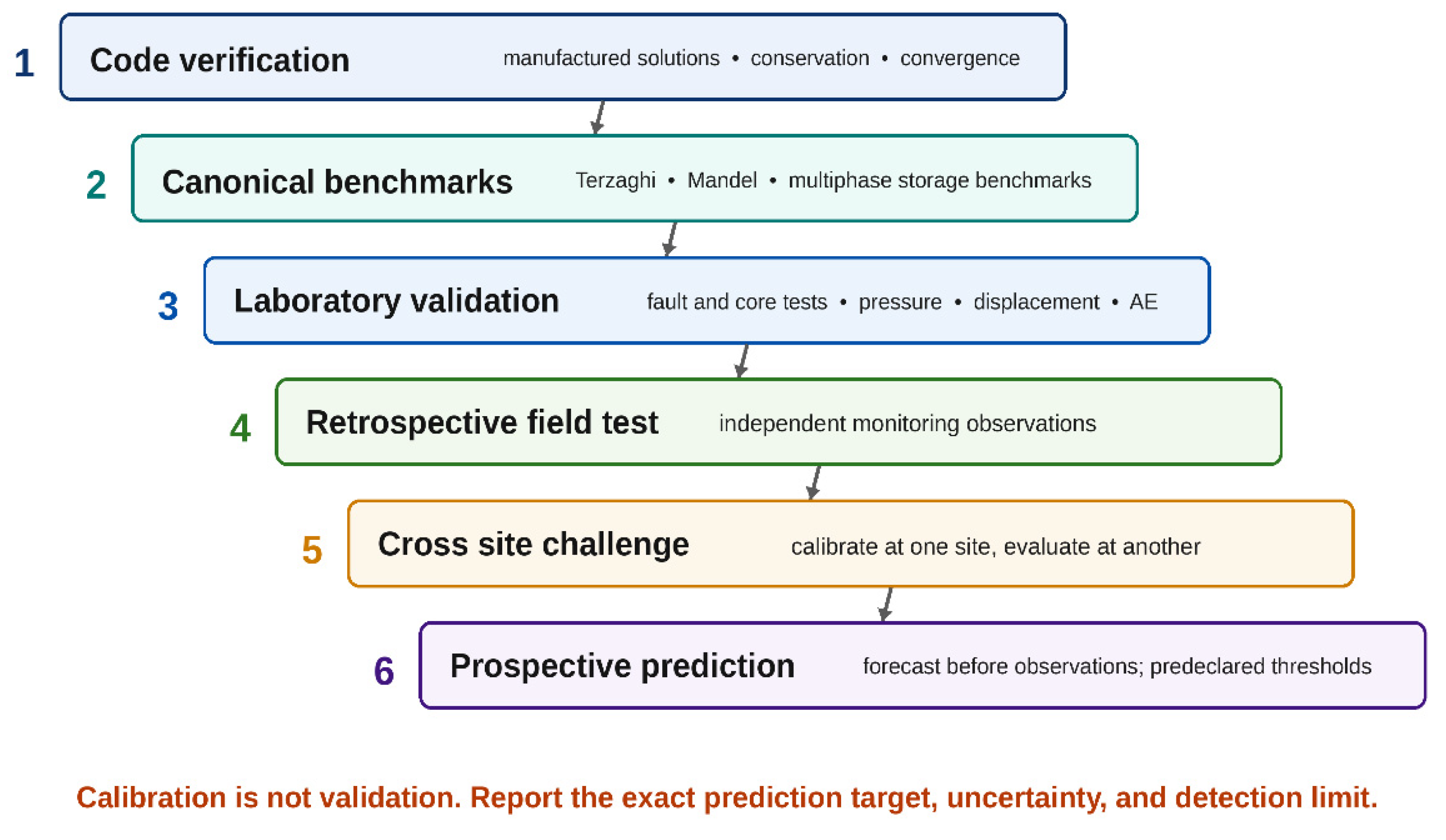
10.4. Verification, Validation, and Credibility Assessment
Figure 9 presents a validation ladder. Each level adds exposure to real world uncertainty. Code verification and canonical benchmarks are necessary but insufficient. Laboratory tests evaluate constitutive response. Retrospective field tests evaluate a site model against independent observations. Cross site tests evaluate transfer. Prospective prediction is the strongest evidence for operational forecasting.
Credibility is context dependent. A model may be credible for screening but not for automatic control. A simple analytical model can be highly credible for a bounded calculation, while a complex digital twin may be poorly credible if its data and algorithms are opaque. The acceptable evidence level increases with the consequence and autonomy of the decision. Table 8 provides the minimum reporting items needed to judge model credibility for the intended decision context.
10.5. Open Data and Benchmark Problems
Progress is limited by the small number of openly accessible field datasets that combine injection history, pressure, deformation, velocity models, event catalogs, waveforms, and geological models. CO₂ DataShare and NRAP resources are important foundations. Open benchmark cases should include synthetic problems with known solutions, laboratory datasets with raw signals and boundary conditions, and field challenges with blind or prospective targets [30].
A useful benchmark suite would contain: (1) single phase poroelastic verification; (2) nonisothermal two phase injection with a known manufactured or reference solution; (3) a frictional interface with pressure dependent slip; (4) shear induced aperture evolution; (5) a dynamic rupture patch initialized by a coupled model; (6) a laboratory core with pressure, displacement, permeability, and acoustic data; and (7) an anonymized field case with predeclared forecast windows. Participants should submit pressure, stress, slip, mass balance, computation time, and uncertainty not only images.
10.6. Reproducible Machine Learning
Machine learning studies should release data splits or identifiers, preprocessing, model code, hyperparameters, random seeds, and calibration procedures. If data are proprietary, a synthetic or deidentified benchmark and executable container can still support reproducibility. Model cards should state training domain, intended use, prohibited use, performance by subgroup/site, detection limit, uncertainty behavior, and known failure modes.
Comparisons should use common baselines and identical splits. Hyperparameter tuning must be nested within training data; using the test set repeatedly turns it into validation data. Reported performance should include variation across seeds and sites. A single best run is insufficient for a safety relevant claim.
10.7. Identifiability, Equifinality, and Model Discrepancy
Calibration can reduce data misfit without uniquely identifying the subsurface. Different combinations of permeability, compressibility, boundary condition, fault transmissivity, elastic modulus, and well representation may reproduce the same pressure history. Surface deformation may constrain a different combination of parameters than pressure, while microseismicity may be sensitive to stress and fault structure that have little influence on plume monitoring. This many to one mapping is commonly described as equifinality and is central to storage geomechanics.
Identifiability should be evaluated before interpreting calibrated parameters physically. Local sensitivity or the Fisher information matrix can reveal nearly collinear parameter effects around a calibrated solution. Global sensitivity and ensemble plots can reveal broader nonlinear tradeoffs. Posterior distributions that remain close to their priors indicate that the observations did not constrain the parameter, even if the best fit simulation looks convincing. Conversely, a narrow posterior can still be misleading if the model structure excludes plausible alternatives.
Model discrepancy represents persistent difference between the governing model and the real system. Examples include unresolved fault segmentation, an incorrect far field boundary, neglected geochemical weakening, simplified wellbore hydraulics, or an inaccurate seismic velocity model. Treating all discrepancy as parameter error drives calibration toward compensating values and can degrade extrapolation. A transparent uncertainty analysis therefore separates measurement error, parameter uncertainty, scenario uncertainty, numerical error, and model form discrepancy as far as the data permit [95].
Multiple data types improve identifiability when they constrain different processes. Pressure constrains transmissivity and storage; temperature constrains thermal transport and wellbore effects; InSAR or tilt constrains deformation and mechanical layering; plume imaging constrains saturation distribution; seismicity constrains active structures and stressing history; tracers constrain connectivity. Joint calibration should preserve the error model and resolution of each dataset rather than forcing all observations into one unweighted least squares objective.
Prediction focused calibration may be preferable to parameter focused calibration. The purpose of the model is often to bound pressure at a fault, probability of slip, plume conformance, or leakage consequence, not to recover a unique permeability field. Ensembles can be accepted when they reproduce relevant observations and then propagated to the decision metric. The result should report the spread, dominant scenario branches, and sensitivity to structural assumptions. This approach recognizes that several subsurface descriptions may remain plausible while still allowing a robust operating decision.
11. Toward Risk Informed Digital Twins and Operational Decision Support
11.1. Digital Twin Requirements
A storage digital twin should contain a state model, observation operators, data assimilation, forecast capability, uncertainty propagation, decision rules, and an audit trail. It should ingest pressure, injection, temperature, deformation, seismic, and other monitoring streams with quality control. It should update uncertain states and parameters rather than merely display new data. Forecasts should include confidence or credible intervals and indicate when the system is outside the validated domain.
The twin can operate at multiple fidelities. Fast surrogates support frequent updates, while full order simulations are rerun periodically or when the system enters a new regime. Reduced order models are recalibrated when discrepancy grows. Human operators review recommendations under preapproved traffic light and pressure management protocols. Human supervised adaptive control should be considered only after extensive prospective validation, explicit fallback testing, and regulatory approval.
Figure 10 presents an observe, update, forecast, decide, and operate loop and a staged research progression. Near term priorities are open benchmarks and uncertainty standards; midterm priorities are cross site validation and reliable hybrid surrogates. The progression is aspirational rather than a technology readiness assessment of currently deployed CO₂ storage systems. Operational maturity requires auditable, human supervised adaptive control and a demonstrated ability to abstain or revert to conservative rules when data or models are outside their validated domain.
11.2. Pressure Management and Optimization
Operational controls include injection rate, bottomhole pressure, injection temperature, distribution among wells, shut in timing, and brine production. Optimization should respect hard constraints on equipment and regulatory pressure and probabilistic constraints on fault activation, uplift, or leakage. Robust optimization considers worst case or distributionally uncertain scenarios rather than optimizing only the mean geological model.
Surrogate assisted optimization can evaluate many schedules, but candidate schedules should be verified with the full order model before implementation. Reinforcement learning is a possible method for sequential control, yet published demonstrations are largely simulation studies. A learned policy may exploit simulator artifacts or fail under unmodeled geology. Safe application requires constrained actions, outside domain detection, fallback rules, and human approval.
11.3. Monitoring Design as an Optimization Problem
Sensor placement should be designed around decision relevant uncertainty. Pressure gauges constrain hydraulic connectivity; deformation sensors constrain spatial pressurization and mechanical structure; borehole seismic arrays improve detection and location; DAS provides dense sampling but complex directional response; temperature and tracers constrain flow pathways. An optimal design may differ depending on whether the target is plume conformance, fault activation, or leakage.
Value of information analysis can compare the expected reduction in decision uncertainty from alternative sensors. The observation operator and expected noise must be included. A large data volume is not automatically informative if it does not constrain the dominant risk parameters.
11.4. Regulatory and Governance Considerations
Regulators require traceable assumptions, conservative operating limits, documented uncertainty, and evidence that monitoring can detect departures from expected behavior. Machine learning components add requirements for data provenance, version control, performance monitoring, explainability, cybersecurity, and change management. A model update that changes an operating recommendation should be reproducible from archived inputs and code. For fault reactivation management, injection rate reduction, well reallocation, brine production, and shut in recommendations should be traceable to specific observations, model versions, uncertainty changes, and approved thresholds.
Human oversight should be substantive. Operators need to understand why a recommendation changed, which observations drove the update, how uncertainty evolved, and what fallback action is available. Explainability should focus on decision relevant evidence rather than decorative feature plots. A transparent simple model may be preferable to a marginally more accurate opaque model for a regulatory decision.
11.5. Human Factors, Communication, and Operational Uncertainty
A decision support system is embedded in an organization, not only in a computer. Data latency, sensor outages, changing catalog completeness, maintenance, handover between shifts, and uncertainty in well controls can influence operational response as strongly as model choice. Procedures should specify who reviews an alert, which independent measurements are checked, how quickly a decision is required, and what conservative action applies when the model or data stream is unavailable.
Risk communication should separate observable facts, model inferences, and management decisions. For example, “event rate increased,” “the posterior probability of slip on fault F3 increased,” and “injection will be reduced by 20%” are different statements with different evidential status. Dashboards that collapse them into one red, yellow, and green indicator can obscure uncertainty. Operators and regulators should be able to inspect the underlying observations, model version, assumptions, and threshold logic.
Operational uncertainty also includes the realized injection schedule. Wellhead rate is not identical to formation rate during transients, and bottomhole pressure may depend on temperature, phase behavior, tubing friction, and wellbore storage. Planned rate changes can be delayed or distributed unevenly among perforations. Forecast ensembles should therefore use measured bottomhole conditions when available and represent control uncertainty when evaluating narrow pressure margins.
Human supervised automation is the appropriate near term objective. Machine learning can reduce data volume, flag anomalies, and rank scenarios; reduced order models can update forecasts rapidly; and optimization can propose pressure management actions. Final authority should remain with qualified personnel operating under approved procedures, with explicit fallback rules and post event review. This governance is not an obstacle to digital twins; it is part of their technical credibility.
12. Research Gaps and Roadmap
12.1. Stress and Fault Characterization
The dominant near term scientific need is improved characterization of the initial stress field and fault architecture. Three dimensional seismic interpretation should be integrated with image logs, well tests, focal mechanisms, and regional stress information. Alternative structural models should be carried through risk analysis. Fault hydraulic connectivity and segmentation are as important as mapped orientation.
Research should quantify how uncertainty in fault geometry propagates to pressure, stress, and rupture predictions. Ensemble structural modeling and graph based representations can support this task. Field campaigns should prioritize measurements that reduce uncertainty in the faults controlling the pressure constrained storage capacity.
12.2. Constitutive Behavior Under Storage Conditions
Rate and state parameters, dilation, permeability evolution, and healing should be measured for representative fault gouges and surfaces under relevant effective stress, temperature, brine salinity, and CO₂ rich fluid conditions. Tests should include velocity steps, holds, pressure transients, and repeated cycles. Smooth saw cuts are useful for reproducibility but must be complemented by rough and natural faults.
A shared laboratory benchmark with raw mechanical, hydraulic, and acoustic data would allow consistent comparison of contact, plasticity, rate and state, damage, and machine learning models. Scale effects should be examined through specimens of different dimensions and through numerical upscaling.
12.3. Coupled THMC and Fault Flow Validation
Chemo mechanical feedback remains weakly constrained. Long duration experiments should measure how mineral reaction changes friction, cohesion, aperture, and multiphase capillary behavior. Fault flow experiments should distinguish core, damage zone, and intersection pathways. Models should represent both pressure relief and leakage consequences of dilation.
12.4. Prospective Field Challenges
The field needs prospective, predeclared challenges. Before an injection phase, teams should submit forecasts of pressure, deformation, event rate, spatial migration, and threshold exceedance with uncertainty. Observations should then be released according to a predefined schedule. This design avoids hindsight and reveals true forecast skill.
Cross site challenges should train or calibrate models at one site and evaluate them at another. The goal is not to find a universally best model but to identify which mechanisms and data support transfer and when site specific recalibration is unavoidable.
12.5. Scientific Machine Learning Priorities
PINN research should focus on discontinuous interfaces, multiphase constitutive behavior, adaptive loss balancing, and credible uncertainty. Neural operator research should emphasize irregular geometry, fault networks, conservation, and goal oriented threshold accuracy. Surrogate studies should publish the training design, parameter domain, full order verification, and outside distribution behavior.
Hybrid systems should exploit complementary strengths: physics for conservation and extrapolation, observations for state updating, and machine learning for rapid emulation and signal processing. Claims should be benchmarked against strong conventional solvers and simple statistical baselines.
12.6. Operational and Social Priorities
Technical systems should be co designed with operators, regulators, and communities. Forecast outputs must correspond to understandable actions and consequences. Monitoring plans should specify public communication protocols for unexpected seismicity or deformation. Research on model performance should be accompanied by research on governance, uncertainty communication, and trust. Table 9 consolidates the priority research needs, near term deliverables, and evidence required before operational use.
13. Discussion
13.1. What Can Be Predicted Reliably Today?
Current methods have comparatively high maturity for calculating pressure and deformation in sufficiently characterized systems, provided that phase behavior, boundaries, constitutive assumptions, and calibration are appropriate for the prediction target. They can screen fault orientation, estimate pressure margins across alternative stress states, and identify scenarios in which thermal effects or hydraulic connectivity require higher fidelity analysis. Seismic signal detection and phase picking can also outperform manual processing in many settings, although site specific detection limits and false alarm rates remain essential.
Reliability decreases as the target moves from reservoir state to dynamic rupture. First slip predictions are highly sensitive to initial stress and friction. Slip evolution requires constitutive parameters that are rarely measured at field scale. Maximum magnitude depends on fault connectivity and rupture arrest that cannot be inferred from pressure alone. A model can therefore be useful for risk reduction without being able to predict the exact time and magnitude of an earthquake.
13.2. Why More Complex Models Do Not Automatically Reduce Risk Uncertainty
Adding physics can reduce structural bias, but it adds parameters. A fully coupled THMC model with poorly constrained reaction and fault parameters may have wider and less identifiable uncertainty than a simpler HM model. Complexity is justified when it changes a decision or explains observations that a simpler model cannot. Model comparison should assess predictive performance and uncertainty, not only process completeness.
The same principle applies to machine learning. A transformer can process long sequences, but it cannot compensate for a catalog with inconsistent detection, a stress field with no constraints, or a training set that lacks representative failures. Scientific machine learning is most valuable when it targets a computational bottleneck or inverse problem and when the physics and data each constrain different uncertainties.
13.3. A Recommended Integrated Workflow
A defensible project workflow begins with a fault and stress inventory and an ensemble of structural interpretations. Analytical screening identifies potentially critical faults and pressure margins. A regional multiphase model evaluates pressure interference and plume evolution. Selected scenarios are coupled to geomechanics with alternative constitutive and boundary assumptions. Laboratory tests constrain friction, dilation, and permeability. Monitoring design is optimized for the uncertainties that control the decision.
During injection, quality controlled pressure, deformation, and seismic observations update the ensemble. Machine learning supports detection and data reduction. Surrogates accelerate ensemble forecasts. Full order models verify candidate operating changes. Risk metrics are communicated with uncertainty and compared with approved thresholds. Unexpected observations trigger model discrepancy analysis and, if necessary, conservative operational action.
This workflow treats modeling as a continuing evidence process rather than a single before injection report. It also prevents a common failure: allowing one calibrated model to become the unquestioned representation of the site.
13.4. Implications for Sustainable Scale Up of Geological CO₂ Storage
Fault reactivation management is a sustainability requirement because durable containment, public confidence, regulatory continuity, and efficient use of subsurface pore space determine whether geological storage can scale. Excessively conservative deterministic pressure limits may strand usable capacity, whereas poorly constrained limits can increase the probability of seismic, integrity, or leakage consequences. The appropriate objective is therefore not maximum injection rate, but maximum verified stored mass subject to containment, geomechanical, monitoring, and societal constraints [1,2,3,5].
Uncertainty aware pressure management can support this balance through multiwell allocation, brine production, monitoring value of information analysis, and predeclared response rules. Hybrid model and data systems may reduce unnecessary shutdowns by distinguishing whether an anomaly is consistent with benign elastic deformation, localized aseismic slip, or a change in containment risk. These benefits depend on transparent uncertainty, prospective testing, and human accountability; otherwise automation may undermine rather than strengthen confidence in geological storage [29,30].
Accordingly, the sustainability contribution of multiphysics and scientific machine learning lies in enabling auditable decisions across the project life cycle, from site selection and injection design to operation, after injection monitoring, and long term stewardship, rather than in algorithmic complexity alone.
14. Conclusions
Fault reactivation during geological CO₂ storage is a coupled state estimation, forecasting, and decision problem. Pressure reduces effective normal stress, but poroelastic total stress change, thermal contraction, multiphase flow, fault connectivity, frictional stability, and permeability evolution determine the response. Stability screening, first slip, aseismic slip, dynamic rupture, seismicity rate, monitoring classification, and leakage consequence are distinct targets and must not be evaluated with a single model or metric.
Continuum reservoir geomechanics models have the greatest present maturity for site scale pressure, stress, and deformation assessment. Interface, discontinuum, DFN, XFEM, and phase field formulations add value when explicit faults, connectivity, large displacement, or fracture growth control the target. No formulation is universally superior; credibility depends on governing equations, constitutive calibration, structural alternatives, boundary conditions, conservation, convergence, and independent observations.
Machine learning is already useful for event detection, phase picking, waveform processing, surrogate simulation, and data assimilation. Physics informed neural networks, neural operators, and reduced order models can accelerate inverse analysis and repeated evaluation, but their strongest evidence remains within bounded training and validation domains. Rare event metrics, probability calibration, leakage safe partitions, conservation checks, threshold accuracy, held out sites, and outside distribution rules are required before operational claims are justified.
The principal barriers to prospective fault slip and seismicity forecasting are uncertain in situ stress, unresolved fault architecture and hydraulic connectivity, limited CO₂ conditioned friction and permeability data, monitoring detection limits, model discrepancy, and sparse cross site evidence. Laboratory performance, natural earthquake detection, and retrospective history matching are valuable evidence but are not substitutes for predeclared field forecasts.
Progress should prioritize open verification benchmarks, shared fault flow experiments, ensemble structural models, common cross site tasks, and prospective field challenges. A digital twin system should be considered operationally mature only when its prediction target, valid domain, uncertainty, failure modes, abstention rules, and decision governance are transparent. Under those conditions, multiphysics and scientific machine learning can support sustainable scale up by improving pressure management and monitoring without replacing verified simulators or qualified human judgment.
Author Contributions
Godsway Akpabli: Conceptualization, Formal analysis, Investigation, Methodology, Software, Visualization, Writing, original draft. Hamid Rahnema: Project administration, Resources, Supervision, Writing, review and editing. Kelvin Hayford: Conceptualization, Formal analysis, Investigation, Methodology, Writing, original draft. William Apau Marfo: Writing, review and editing. Kwamena Opoku Duartey: Writing, review and editing. Joseph Osei-Nsankyire: Writing, review and editing. All authors have read and agreed to the published version of the manuscript.
Funding
Not applicable.
Institutional Review Board Statement
Not applicable.
Informed Consent Statement
Not applicable.
Data Availability Statement
No new data were created or analyzed in this study. All information synthesized in this review is available from the cited literature. Original editable versions of the authors’ synthesis figures are available from the corresponding author upon reasonable request.
Conflicts of Interest
The authors declare that they have no known competing financial or non-financial interests that could have influenced the work reported in this article.
Acknowledgments
The authors acknowledge New Mexico Institute of Mining and Technology for providing institutional resources that supported this work.
References
- IPCC. Climate change 2022: mitigation of climate change. Contribution of Working Group III to the Sixth Assessment Report of the Intergovernmental Panel on Climate Change; Cambridge University Press: Cambridge, 2022. [Google Scholar] [CrossRef]
- IEA. Net zero by 2050: a roadmap for the global energy sector; International Energy Agency: Paris, 2021. [Google Scholar]
- Global CCS Institute. Global status of CCS 2025; Global CCS Institute: Melbourne, 2025. [Google Scholar]
- Rutqvist, J. The geomechanics of CO2 storage in deep sedimentary formations. Geotech. Geol. Eng. 2012, 30, 525–551. [Google Scholar] [CrossRef]
- White, J.A.; Foxall, W. Assessing induced seismicity risk at CO2 storage projects: recent progress and remaining challenges. Int. J. Greenh. Gas. Control 2016, 49, 413–424. [Google Scholar] [CrossRef]
- Vilarrasa, V.; Carrera, J.; Olivella, S.; Rutqvist, J.; Laloui, L. Induced seismicity in geologic carbon storage. Solid Earth 2019, 10, 871–892. [Google Scholar] [CrossRef]
- Song, Y.; Jun, S.; Na, Y.; Kim, K.; Jang, Y.; Wang, J. Geomechanical challenges during geological CO2 storage: a review. Chem. Eng. J. 2023, 456, 140968. [Google Scholar] [CrossRef]
- Verdon, J.P. Significance for secure CO2 storage of earthquakes induced by fluid injection. Env. Res. Lett. 2014, 9, 064022. [Google Scholar] [CrossRef]
- Verdon, J.P.; Stork, A.L. Carbon capture and storage, geomechanics and induced seismic activity. J. Rock. Mech. Geotech. Eng. 2016, 8, 928–935. [Google Scholar] [CrossRef]
- I.E.A.G.H.G. Reviewing the implications of unlikely but potential CO2 migration to the surface or shallow subsurface; Technical Report 2025-01; IEA Greenhouse Gas R&D Programme: Cheltenham, 2025. [Google Scholar] [CrossRef] [PubMed]
- Cappa, F.; Rutqvist, J. Modeling of coupled deformation and permeability evolution during fault reactivation induced by deep underground injection of CO2. Int. J. Greenh. Gas. Control 2011, 5, 336–346. [Google Scholar] [CrossRef]
- Jha, B.; Juanes, R. Coupled multiphase flow and poromechanics: a computational model of pore pressure effects on fault slip and earthquake triggering. Water Resour. Res. 2014, 50, 3776–3808. [Google Scholar] [CrossRef]
- Vilarrasa, V.; Rutqvist, J. Thermal effects on geologic carbon storage. Earth-Sci. Rev. 2017, 165, 245–256. [Google Scholar] [CrossRef]
- Karniadakis, G.E.; Kevrekidis, I.G.; Lu, L.; Perdikaris, P.; Wang, S.; Yang, L. Physics-informed machine learning. Nat. Rev. Phys. 2021, 3, 422–440. [Google Scholar] [CrossRef]
- Geertsma, J. Land subsidence above compacting oil and gas reservoirs. J. Pet. Technol. 1973, 25, 734–744. [Google Scholar] [CrossRef]
- Segall, P. Earthquakes triggered by fluid extraction. Geology 1989, 17, 942–946. [Google Scholar] [CrossRef]
- Rutqvist, J.; Wu, Y.S.; Tsang, C.F.; Bodvarsson, G. A modeling approach for analysis of coupled multiphase fluid flow, heat transfer, and deformation in fractured porous rock. Int. J. Rock. Mech. Min. Sci. 2002, 39, 429–442. [Google Scholar] [CrossRef]
- Settari, A.; Walters, D.A. Advances in coupled geomechanical and reservoir modeling with applications to reservoir compaction. SPE J. 2001, 6, 334–342. [Google Scholar] [CrossRef]
- Kim, J.; Tchelepi, H.A.; Juanes, R. Stability and convergence of sequential methods for coupled flow and geomechanics: fixed-stress and fixed-strain splits. Comput Methods Appl. Mech. Eng. 2011, 200, 1591–1606. [Google Scholar] [CrossRef]
- Gaston, D.; Newman, C.; Hansen, G.; Lebrun-Grandié, D. MOOSE: a parallel computational framework for coupled systems of nonlinear equations. Nucl. Eng. Des. 2009, 239, 1768–1778. [Google Scholar] [CrossRef]
- Rouet-Leduc, B.; Hulbert, C.; Lubbers, N.; Barros, K.; Humphreys, C.J.; Johnson, P.A. Machine learning predicts laboratory earthquakes. Geophys Res. Lett. 2017, 44, 9276–9282. [Google Scholar] [CrossRef]
- Bergen, K.J.; Johnson, P.A.; de Hoop, M.V.; Beroza, G.C. Machine learning for data-driven discovery in solid Earth geoscience. Science 2019, 363, eaau0323. [Google Scholar] [CrossRef] [PubMed]
- Kong, Q.; Trugman, D.T.; Ross, Z.E.; Bianco, M.J.; Meade, B.J.; Gerstoft, P. Machine learning in seismology: turning data into insights. Seismol. Res. Lett. 2019, 90, 3–14. [Google Scholar] [CrossRef]
- Mousavi, S.M.; Ellsworth, W.L.; Zhu, W.; Chuang, L.Y.; Beroza, G.C. Earthquake Transformer - an attentive deep-learning model for simultaneous earthquake detection and phase picking. Nat. Commun. 2020, 11, 3952. [Google Scholar] [CrossRef] [PubMed]
- Mousavi, S.M.; Beroza, G.C. Machine learning in earthquake seismology. Annu Rev. Earth Planet Sci. 2023, 51, 105–129. [Google Scholar] [CrossRef]
- Raissi, M.; Perdikaris, P.; Karniadakis, G.E. Physics-informed neural networks: a deep learning framework for solving forward and inverse problems involving nonlinear partial differential equations. J. Comput Phys. 2019, 378, 686–707. [Google Scholar] [CrossRef]
- Willard, J.; Jia, X.; Xu, S.; Steinbach, M.; Kumar, V. Integrating scientific knowledge with machine learning for engineering and environmental systems. ACM Comput Surv. 2022, 55, 1–37. [Google Scholar] [CrossRef]
- Millevoi, C.; Spiezia, N.; Ferronato, M. On physics-informed neural networks training for coupled hydro-poromechanical problems. J. Comput Phys. 2024, 516, 113299. [Google Scholar] [CrossRef]
- Mignan, A.; Broccardo, M.; Wiemer, S.; Giardini, D. Induced seismicity closed-form traffic light system for actuarial decision-making during deep fluid injections. Sci. Rep. 2017, 7, 13607. [Google Scholar] [CrossRef] [PubMed]
- Vasylkivska, V.; Dilmore, R.; Lackey, G.; Zhang, Y.; King, S.; Bacon, D.; Chen, B.; Mansoor, K.; Harp, D. NRAP-open-IAM: a flexible open-source integrated-assessment-model for geologic carbon storage risk assessment and management. Env. Model Softw. 2021, 143, 105114. [Google Scholar] [CrossRef]
- Morris, A.; Ferrill, D.A.; Henderson, D.B. Slip-tendency analysis and fault reactivation. Geology 1996, 24, 275–278. [Google Scholar] [CrossRef]
- McGarr, A. Maximum magnitude earthquakes induced by fluid injection. J. Geophys Res. Solid Earth 2014, 119, 1008–1019. [Google Scholar] [CrossRef]
- Vilarrasa, V.; Carrera, J. Geologic carbon storage is unlikely to trigger large earthquakes and reactivate faults through which CO2 could leak. Proc. Natl. Acad. Sci. USA 2015, 112, 5938–5943. [Google Scholar] [CrossRef] [PubMed]
- Rinaldi, A.P.; Rutqvist, J.; Cappa, F. Geomechanical effects on CO2 leakage through fault zones during large-scale underground injection. Int. J. Greenh. Gas. Control 2014, 20, 117–131. [Google Scholar] [CrossRef]
- Meguerdijian, S.; Pawar, R.J.; Chen, B.; Jha, B.; Gable, C.W.; Miller, T.A. Physics-informed machine learning for fault-leakage reduced-order modeling. Int. J. Greenh. Gas. Control 2023, 125, 103873. [Google Scholar] [CrossRef]
- Bommer, J.J.; Oates, S.; Cepeda, J.M.; Lindholm, C.; Bird, J.; Torres, R.; Marroquín, G.; Rivas, J. Control of hazard due to seismicity induced by a hot fractured rock geothermal project. Eng. Geol. 2006, 83, 287–306. [Google Scholar] [CrossRef]
- Biot, M.A. General theory of three-dimensional consolidation. J. Appl. Phys. 1941, 12, 155–164. [Google Scholar] [CrossRef]
- Rice, J.R.; Cleary, M.P. Some basic stress diffusion solutions for fluid-saturated elastic porous media with compressible constituents. Rev. Geophys 1976, 14, 227–241. [Google Scholar] [CrossRef]
- Wang, H.F. Theory of linear poroelasticity with applications to geomechanics and hydrogeology; Princeton University Press: Princeton, 2000. [Google Scholar]
- King, G.C.P.; Stein, R.S.; Lin, J. Static stress changes and the triggering of earthquakes. Bull. Seismol. Soc. Am. 1994, 84, 935–953. [Google Scholar] [CrossRef]
- Segall, P.; Lu, S. Injection-induced seismicity: poroelastic and earthquake nucleation effects. J. Geophys Res. Solid Earth 2015, 120, 5082–5103. [Google Scholar] [CrossRef]
- Neuzil, C.E. Hydromechanical coupling in geologic processes. Hydrogeol. J. 2003, 11, 41–83. [Google Scholar] [CrossRef]
- Birkholzer, J.T.; Oldenburg, C.M.; Zhou, Q. CO2 migration and pressure evolution in deep saline aquifers. Int. J. Greenh. Gas. Control 2015, 40, 203–220. [Google Scholar] [CrossRef]
- Gor, G.Y.; Elliot, T.R.; Prévost, J.H. Effects of thermal stresses on caprock integrity during CO2 storage. Int. J. Greenh. Gas. Control 2013, 12, 300–309. [Google Scholar] [CrossRef]
- Vilarrasa, V.; Olivella, S.; Carrera, J.; Rutqvist, J. Long term impacts of cold CO2 injection on the caprock integrity. Int. J. Greenh. Gas. Control 2014, 24, 1–13. [Google Scholar] [CrossRef]
- Vilarrasa, V.; Laloui, L. Potential fracture propagation into the caprock induced by cold CO2 injection in normal faulting stress regimes. Geomech. Energy Env. 2015, 2, 22–31. [Google Scholar] [CrossRef]
- Dieterich, J.H. Modeling of rock friction: 1. Experimental results and constitutive equations. J. Geophys Res. 1979, 84, 2161–2168. [Google Scholar] [CrossRef]
- Ruina, A. Slip instability and state variable friction laws. J. Geophys Res. 1983, 88, 10359–10370. [Google Scholar] [CrossRef]
- Marone, C. Laboratory-derived friction laws and their application to seismic faulting. Annu Rev. Earth Planet Sci. 1998, 26, 643–696. [Google Scholar] [CrossRef]
- Ikari, M.J.; Marone, C.; Saffer, D.M. On the relation between fault strength and frictional stability. Geology 2011, 39, 83–86. [Google Scholar] [CrossRef]
- Rubin, A.M.; Ampuero, J.P. Earthquake nucleation on (aging) rate and state faults. J. Geophys Res. Solid Earth 2005, 110, B11312. [Google Scholar] [CrossRef]
- Ampuero, J.P.; Rubin, A.M. Earthquake nucleation on rate and state faults - aging and slip laws. J. Geophys Res. Solid Earth 2008, 113, B01302. [Google Scholar] [CrossRef]
- Byerlee, J. Friction of rocks. Pure Appl. Geophys 1978, 116, 615–626. [Google Scholar] [CrossRef]
- Witherspoon, P.A.; Wang, J.S.Y.; Iwai, K.; Gale, J.E. Validity of cubic law for fluid flow in a deformable rock fracture. Water Resour. Res. 1980, 16, 1016–1024. [Google Scholar] [CrossRef]
- Min, K.B.; Rutqvist, J.; Tsang, C.F.; Jing, L. Stress-dependent permeability of fractured rock masses: a numerical study. Int. J. Rock. Mech. Min. Sci. 2004, 41, 1191–1210. [Google Scholar] [CrossRef]
- Lei, Q.; Latham, J.P.; Tsang, C.F. The use of discrete fracture networks for modelling coupled geomechanical and hydrological behaviour of fractured rocks. Comput Geotech. 2017, 85, 151–176. [Google Scholar] [CrossRef]
- Hanks, T.C.; Kanamori, H. A moment magnitude scale. J. Geophys Res. 1979, 84, 2348–2350. [Google Scholar] [CrossRef]
- Dean, R.H.; Gai, X.; Stone, C.M.; Minkoff, S.E. A comparison of techniques for coupling porous flow and geomechanics. SPE J. 2006, 11, 132–140. [Google Scholar] [CrossRef]
- Mikelić, A.; Wheeler, M.F. Convergence of iterative coupling for coupled flow and geomechanics. Comput Geosci. 2013, 17, 455–461. [Google Scholar] [CrossRef]
- Kolditz, O.; Bauer, S.; Bilke, L. OpenGeoSys: an open-source initiative for numerical simulation of thermo-hydro-mechanical/chemical processes in porous media. Env. Earth Sci. 2012, 67, 589–599. [Google Scholar] [CrossRef]
- Rutqvist, J. Status of the TOUGH-FLAC simulator and recent applications related to coupled fluid flow and crustal deformations. Comput Geosci. 2011, 37, 739–750. [Google Scholar] [CrossRef]
- Cundall, P.A.; Strack, O.D.L. A discrete numerical model for granular assemblies. Geotechnique 1979, 29, 47–65. [Google Scholar] [CrossRef]
- Jing, L.; Stephansson, O. Fundamentals of discrete element methods for rock engineering: theory and applications; Elsevier: Amsterdam, 2007. [Google Scholar]
- Lisjak, A.; Grasselli, G. A review of discrete modeling techniques for fracturing processes in discontinuous rock masses. J. Rock. Mech. Geotech. Eng. 2014, 6, 301–314. [Google Scholar] [CrossRef]
- Belytschko, T.; Black, T. Elastic crack growth in finite elements with minimal remeshing. Int. J. Numer Methods Eng. 1999, 45, 601–620. [Google Scholar] [CrossRef]
- Moës, N.; Dolbow, J.; Belytschko, T. A finite element method for crack growth without remeshing. Int. J. Numer Methods Eng. 1999, 46, 131–150. [Google Scholar] [CrossRef]
- Fries, T.P.; Belytschko, T. The extended/generalized finite element method: an overview of the method and its applications. Int. J. Numer Methods Eng. 2010, 84, 253–304. [Google Scholar] [CrossRef]
- Hughes, T.J.R. The finite element method: linear static and dynamic finite element analysis; Dover: Mineola, 2000. [Google Scholar]
- Taron, J.; Elsworth, D.; Min, K.B. Numerical simulation of thermal-hydrologic-mechanical-chemical processes in deformable, fractured porous media. Int. J. Rock. Mech. Min. Sci. 2009, 46, 842–854. [Google Scholar] [CrossRef]
- Lockner, D.A.; Byerlee, J.D.; Kuksenko, V.; Ponomarev, A.; Sidorin, A. Quasi-static fault growth and shear fracture energy in granite. Nature 1991, 350, 39–42. [Google Scholar] [CrossRef]
- Grosse, C.U.; Ohtsu, M. (Eds.) Acoustic emission testing; Springer: Berlin, 2008. [Google Scholar] [CrossRef]
- Lei, X.; Ma, S. Laboratory acoustic emission study for earthquake generation process. Earthq. Sci. 2014, 27, 627–646. [Google Scholar] [CrossRef]
- Vasco, D.W.; Rucci, A.; Ferretti, A.; Novali, F.; Bissell, R.C.; Ringrose, P.S.; Mathieson, A.S.; Wright, I.W. Satellite-based measurements of surface deformation reveal fluid flow associated with the geological storage of carbon dioxide. Geophys Res. Lett. 2010, 37, L03303. [Google Scholar] [CrossRef]
- Rutqvist, J.; Vasco, D.W.; Myer, L. Coupled reservoir-geomechanical analysis of CO2 injection and ground deformations at In Salah, Algeria. Int. J. Greenh. Gas. Control 2010, 4, 225–230. [Google Scholar] [CrossRef]
- Rinaldi, A.P.; Rutqvist, J. Modeling of deep fracture zone opening and transient ground surface uplift at KB-502 CO2 injection well, In Salah, Algeria. Int. J. Greenh. Gas. Control 2013, 12, 155–167. [Google Scholar] [CrossRef]
- Verdon, J.P.; Stork, A.L.; Bissell, R.C.; Bond, C.E.; Werner, M.J. Simulation of seismic events induced by CO2 injection at In Salah, Algeria. Earth Planet Sci. Lett. 2015, 426, 118–129. [Google Scholar] [CrossRef]
- Stork, A.L.; Verdon, J.P.; Kendall, J.M. The microseismic response at the In Salah Carbon Capture and Storage (CCS) site. Int. J. Greenh. Gas. Control 2015, 32, 159–171. [Google Scholar] [CrossRef]
- Bauer, R.A.; Carney, M.; Finley, R.J. Overview of microseismic response to CO2 injection into the Mt. Simon saline reservoir at the Illinois Basin-Decatur Project. Int. J. Greenh. Gas. Control 2016, 54, 378–388. [Google Scholar] [CrossRef]
- Luu, K.; Schoenball, M.; Oldenburg, C.M.; Rutqvist, J. Coupled hydromechanical modeling of induced seismicity from CO2 injection in the Illinois Basin. J. Geophys Res. Solid Earth 2022, 127, e2021JB023496. [Google Scholar] [CrossRef]
- Jenkins, C.; Barraclough, P.; Correa, J. Field tests of geological storage of CO2 at the Otway International Test Centre, Australia: trapping and monitoring the migrating plumes. Geoenergy 2024, 2, geoenergy2023–035. [Google Scholar] [CrossRef]
- Glubokovskikh, S.; Pevzner, R.; Dance, T. A small CO2 leakage may induce seismicity on a sub-seismic fault in a good-porosity clastic saline aquifer. Geophys Res. Lett. 2022, 49, e2022GL098062. [Google Scholar] [CrossRef]
- Furre, A.K.; Eiken, O.; Alnes, H.; Vevatne, J.N.; Kiær, A.F. 20 years of monitoring CO2-injection at Sleipner. Energy Procedia 2017, 114, 3916–3926. [Google Scholar] [CrossRef]
- Hansen, O.; Gilding, D.; Nazarian, B.; Osdal, B.; Ringrose, P.; Kristoffersen, J.B.; Eiken, O.; Hansen, H. Snøhvit: the history of injecting and storing 1 Mt CO2 in the fluvial Tubåen Formation. Energy Procedia 2013, 37, 3565–3573. [Google Scholar] [CrossRef]
- Martens, S.; Liebscher, A.; Möller, F. CO2 storage at the Ketzin pilot site, Germany: fourth year of injection, monitoring, modelling and verification. Energy Procedia 2013, 37, 6434–6443. [Google Scholar] [CrossRef]
- Häring, M.O.; Schanz, U.; Ladner, F.; Dyer, B.C. Characterisation of the Basel 1 enhanced geothermal system. Geothermics 2008, 37, 469–495. [Google Scholar] [CrossRef]
- Bachmann, C.E.; Wiemer, S.; Woessner, J.; Hainzl, S. Statistical analysis of the induced Basel 2006 earthquake sequence: introducing a probability-based monitoring approach for enhanced geothermal systems. Geophys J. Int. 2011, 186, 793–807. [Google Scholar] [CrossRef]
- Perol, T.; Gharbi, M.; Denolle, M. Convolutional neural network for earthquake detection and location. Sci. Adv. 2018, 4, e1700578. [Google Scholar] [CrossRef] [PubMed]
- Ross, Z.E.; Meier, M.A.; Hauksson, E.; Heaton, T.H. Generalized seismic phase detection with deep learning. Bull. Seismol. Soc. Am. 2018, 108, 2894–2901. [Google Scholar] [CrossRef]
- Ogata, Y. Statistical models for earthquake occurrences and residual analysis for point processes. J. Am. Stat. Assoc. 1988, 83, 9–27. [Google Scholar] [CrossRef]
- Kadeethum, T.; Jørgensen, T.M.; Nick, H.M. Physics-informed neural networks for solving nonlinear diffusivity and Biot’s equations. PLoS ONE 2020, 15, e0232683. [Google Scholar] [CrossRef] [PubMed]
- Li, Z.; Kovachki, N.; Azizzadenesheli, K.; Liu, B.; Bhattacharya, K.; Stuart, A.; Anandkumar, A. Fourier neural operator for parametric partial differential equations. International Conference on Learning Representations, 2021. [Google Scholar] [CrossRef]
- Lu, L.; Jin, P.; Pang, G.; Zhang, Z.; Karniadakis, G.E. Learning nonlinear operators via DeepONet based on the universal approximation theorem of operators. Nat. Mach. Intell. 2021, 3, 218–229. [Google Scholar] [CrossRef]
- Wen, G.; Li, Z.; Azizzadenesheli, K.; Anandkumar, A.; Benson, S.M. U-FNO - an enhanced Fourier neural operator-based deep-learning model for multiphase flow. Adv. Water Resour. 2022, 163, 104180. [Google Scholar] [CrossRef]
- Tang, M.; Ju, X.; Durlofsky, L.J. Deep-learning-based coupled flow-geomechanics surrogate model for CO2 sequestration. Int. J. Greenh. Gas. Control 2022, 118, 103692. [Google Scholar] [CrossRef]
- Oberkampf, W.L.; Roy, C.J. Verification and validation in scientific computing; Cambridge University Press: Cambridge, 2010. [Google Scholar] [CrossRef]
Figure 1.
Integrated framework for fault reactivation prediction during geological CO₂ storage. (a) Storage system containing an injection well, reservoir, caprock, basement, and a potentially connected fault. (b) Coupled thermal, hydraulic, and mechanical modeling and monitoring evidence. (c) Scientific machine learning tools and risk informed operational decisions. Original synthesis based on Rutqvist [4], Jha and Juanes [12], White and Foxall [5], Karniadakis et al. [14], and Song et al. [7].
Figure 1.
Integrated framework for fault reactivation prediction during geological CO₂ storage. (a) Storage system containing an injection well, reservoir, caprock, basement, and a potentially connected fault. (b) Coupled thermal, hydraulic, and mechanical modeling and monitoring evidence. (c) Scientific machine learning tools and risk informed operational decisions. Original synthesis based on Rutqvist [4], Jha and Juanes [12], White and Foxall [5], Karniadakis et al. [14], and Song et al. [7].
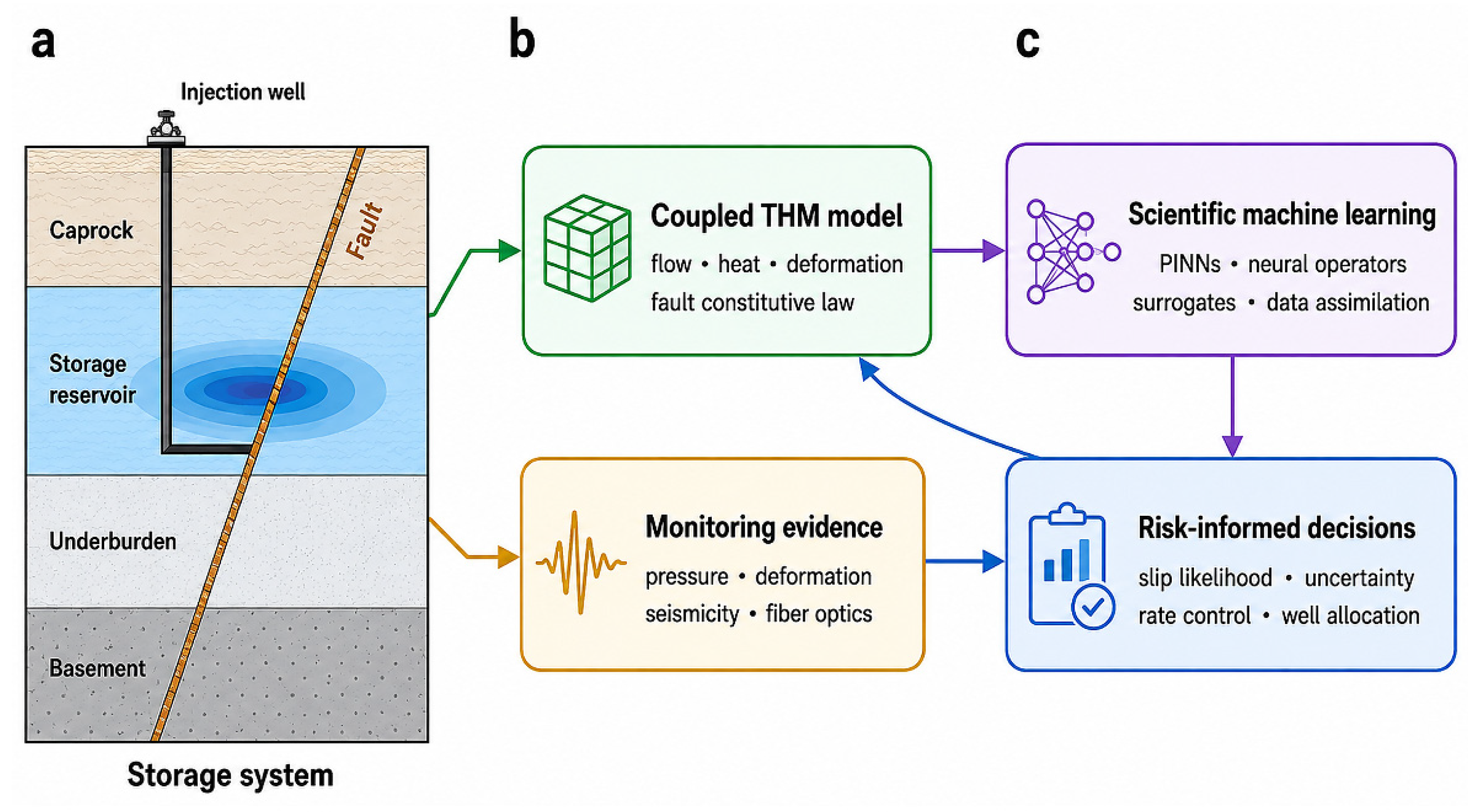
Figure 2.
Mechanistic chain from injection control to reservoir state, fault response, monitoring evidence, and operational action. The return path emphasizes that monitoring and history matching update model state, parameter distributions, and operating limits. Original synthesis based on White and Foxall [5], Mignan et al. [29], and Vasylkivska et al. [30].
Figure 2.
Mechanistic chain from injection control to reservoir state, fault response, monitoring evidence, and operational action. The return path emphasizes that monitoring and history matching update model state, parameter distributions, and operating limits. Original synthesis based on White and Foxall [5], Mignan et al. [29], and Vasylkivska et al. [30].
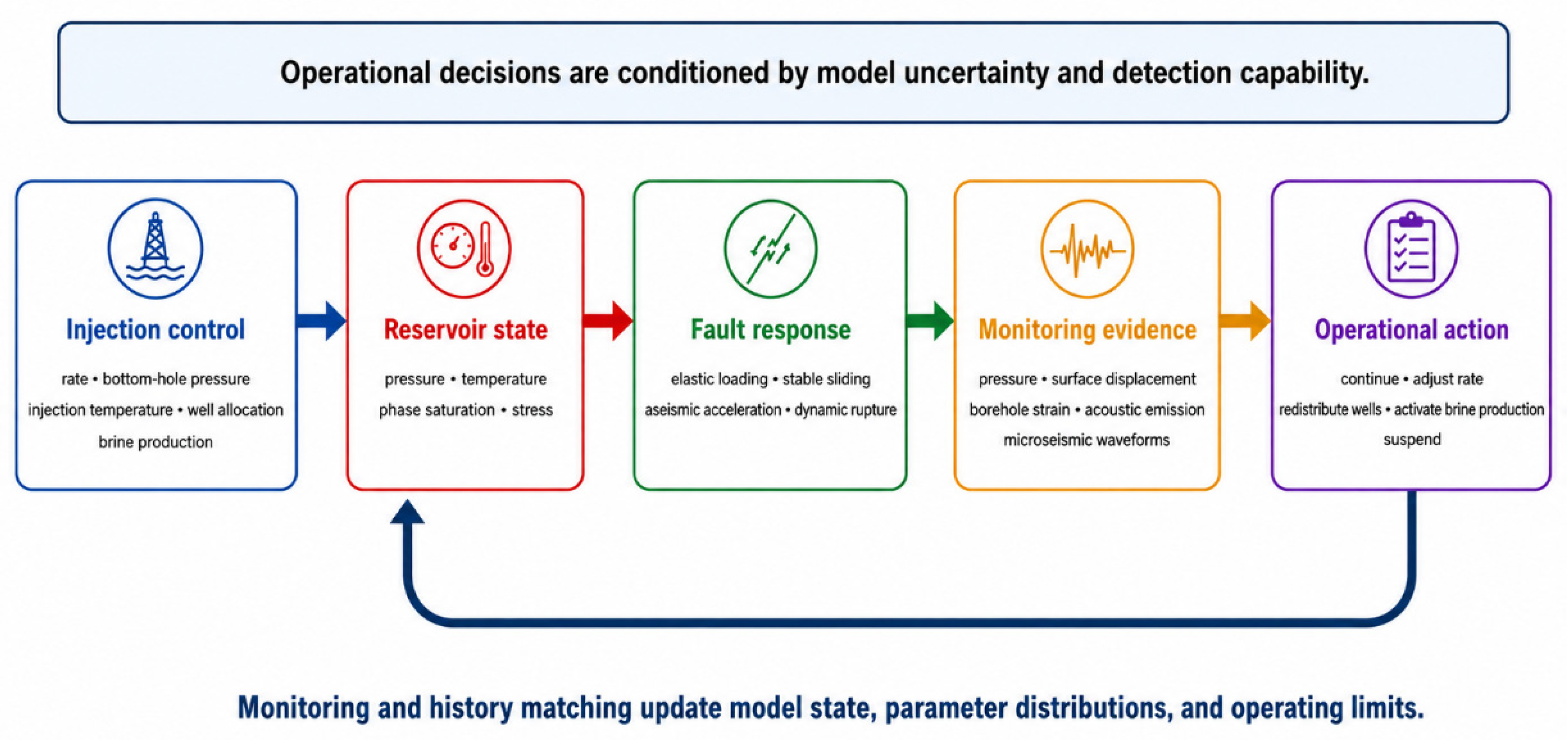
Figure 4.
Coupling architectures for storage geomechanics. (a) One way sequential coupling. (b) Two way staggered coupling with iteration to a defined tolerance. (c) Monolithic solution of flow, heat, deformation, saturation, and fault state variables. Original synthesis based on Settari and Walters [18], Dean et al. [58], Kim et al. [19], and Mikelić and Wheeler [59].
Figure 4.
Coupling architectures for storage geomechanics. (a) One way sequential coupling. (b) Two way staggered coupling with iteration to a defined tolerance. (c) Monolithic solution of flow, heat, deformation, saturation, and fault state variables. Original synthesis based on Settari and Walters [18], Dean et al. [58], Kim et al. [19], and Mikelić and Wheeler [59].
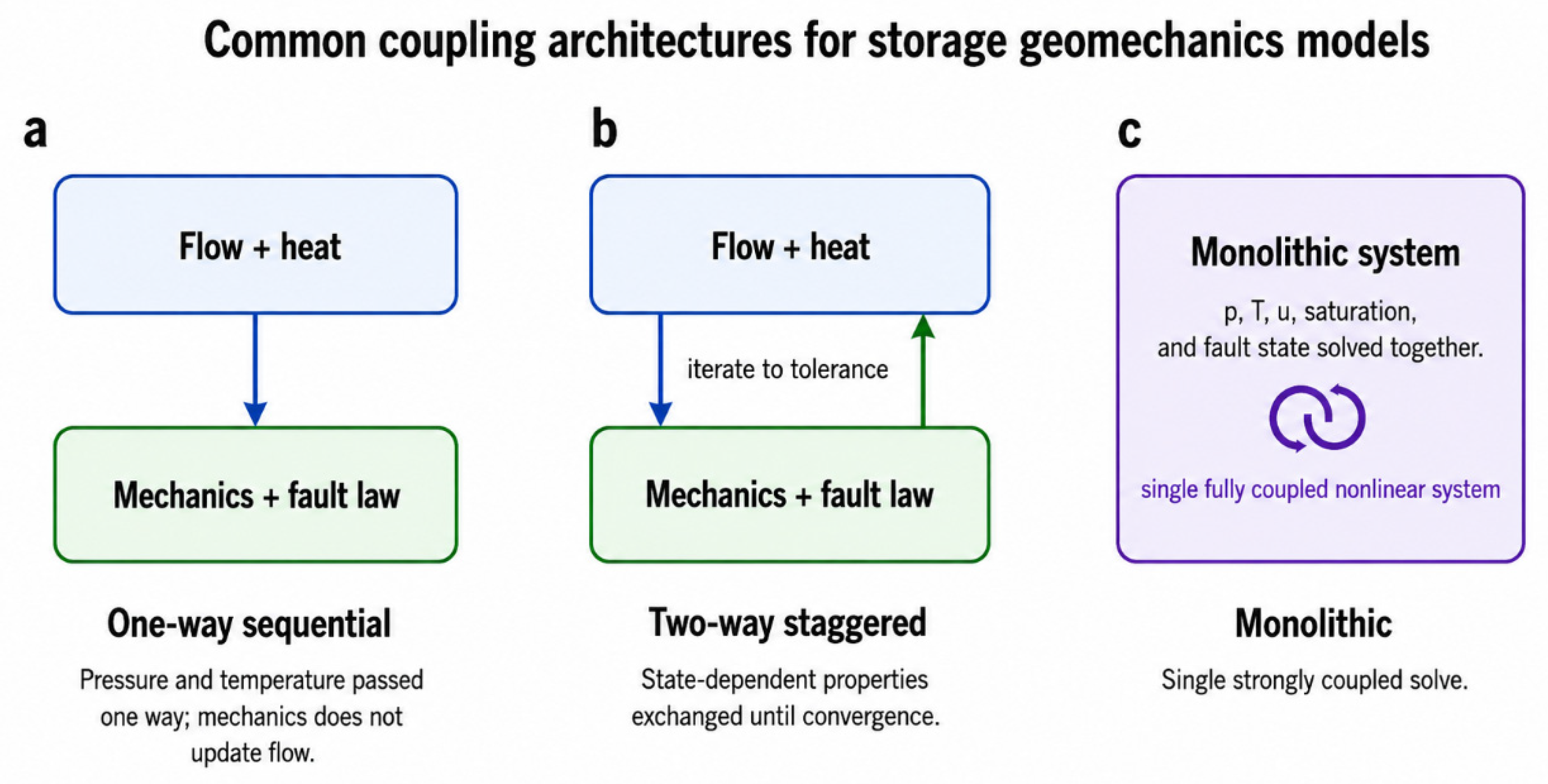
Figure 5.
Qualitative capability matrix for analytical, continuum, discontinuum, fracture, and scientific machine learning methods. The author defined rubric is: 0, capability not intrinsic; 1, possible only with substantial extension or limited evidence; 2, demonstrated with material limitations; and 3, comparatively mature or repeatedly demonstrated for the stated use. Scores do not rank vendors or guarantee site specific performance. The right hand bars indicate characteristic spatial reach. Original synthesis based on Hughes [68], Rutqvist et al. [17], Jing and Stephansson [63], Fries and Belytschko [67], Lei et al. [56], and Karniadakis et al. [14].
Figure 5.
Qualitative capability matrix for analytical, continuum, discontinuum, fracture, and scientific machine learning methods. The author defined rubric is: 0, capability not intrinsic; 1, possible only with substantial extension or limited evidence; 2, demonstrated with material limitations; and 3, comparatively mature or repeatedly demonstrated for the stated use. Scores do not rank vendors or guarantee site specific performance. The right hand bars indicate characteristic spatial reach. Original synthesis based on Hughes [68], Rutqvist et al. [17], Jing and Stephansson [63], Fries and Belytschko [67], Lei et al. [56], and Karniadakis et al. [14].
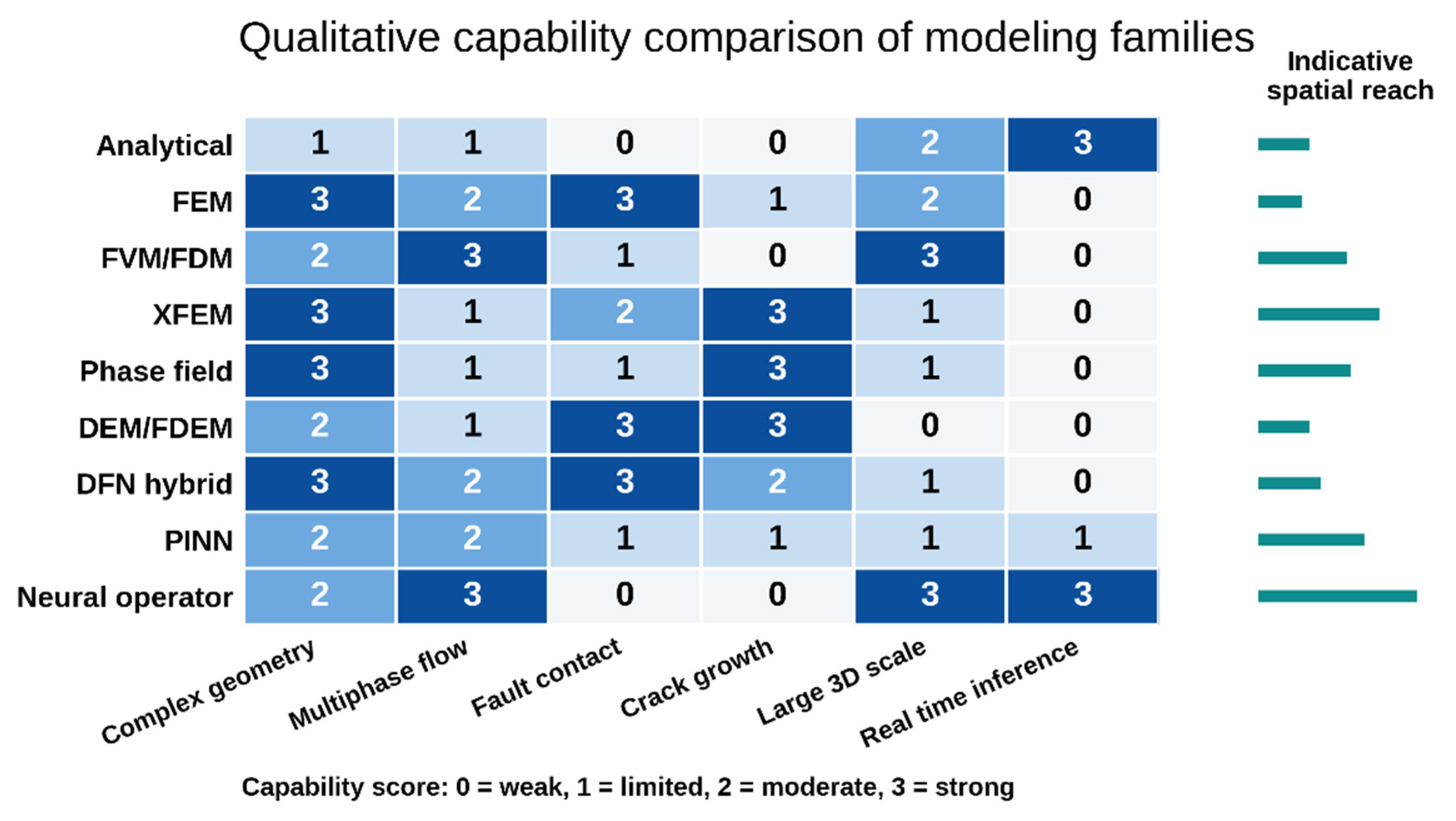
Figure 6.
Qualitative availability of field evidence for evaluating fault reactivation models at In Salah, the Illinois Basin Decatur Project, Otway, and the Basel enhanced geothermal analogue. Strong = multiple independent data types plus peer reviewed model evaluation; moderate = useful but incomplete coverage; limited = sparse observations, restricted monitoring geometry, or no prospective test. Categories describe evidence suitability, not project safety. Synthesis based on Häring et al. [85], Rutqvist et al. [74], Bachmann et al. [86], Stork et al. [77], Bauer et al. [78], Luu et al. [79], Glubokovskikh et al. [81], and Jenkins et al. [80].
Figure 6.
Qualitative availability of field evidence for evaluating fault reactivation models at In Salah, the Illinois Basin Decatur Project, Otway, and the Basel enhanced geothermal analogue. Strong = multiple independent data types plus peer reviewed model evaluation; moderate = useful but incomplete coverage; limited = sparse observations, restricted monitoring geometry, or no prospective test. Categories describe evidence suitability, not project safety. Synthesis based on Häring et al. [85], Rutqvist et al. [74], Bachmann et al. [86], Stork et al. [77], Bauer et al. [78], Luu et al. [79], Glubokovskikh et al. [81], and Jenkins et al. [80].
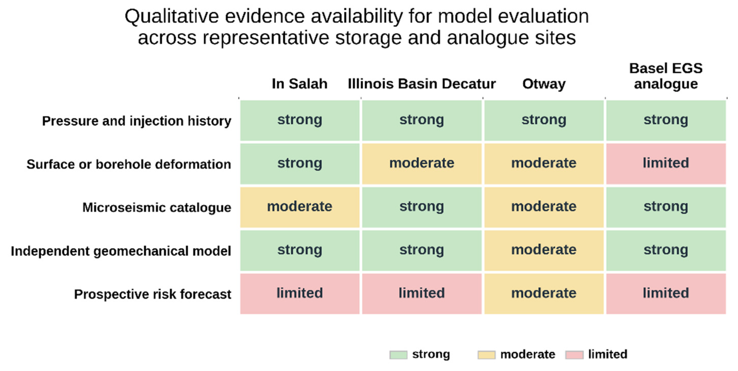
Figure 7.
Machine learning workflow for geomechanical monitoring and prediction. (a) Inputs, model classes, tasks, and outputs. (b) Leakage safe progression from training to external validation and prospective testing. Original synthesis based on Bergen et al. [22], Kong et al. [23], Mousavi et al. [24], and Mousavi and Beroza [25].
Figure 7.
Machine learning workflow for geomechanical monitoring and prediction. (a) Inputs, model classes, tasks, and outputs. (b) Leakage safe progression from training to external validation and prospective testing. Original synthesis based on Bergen et al. [22], Kong et al. [23], Mousavi et al. [24], and Mousavi and Beroza [25].
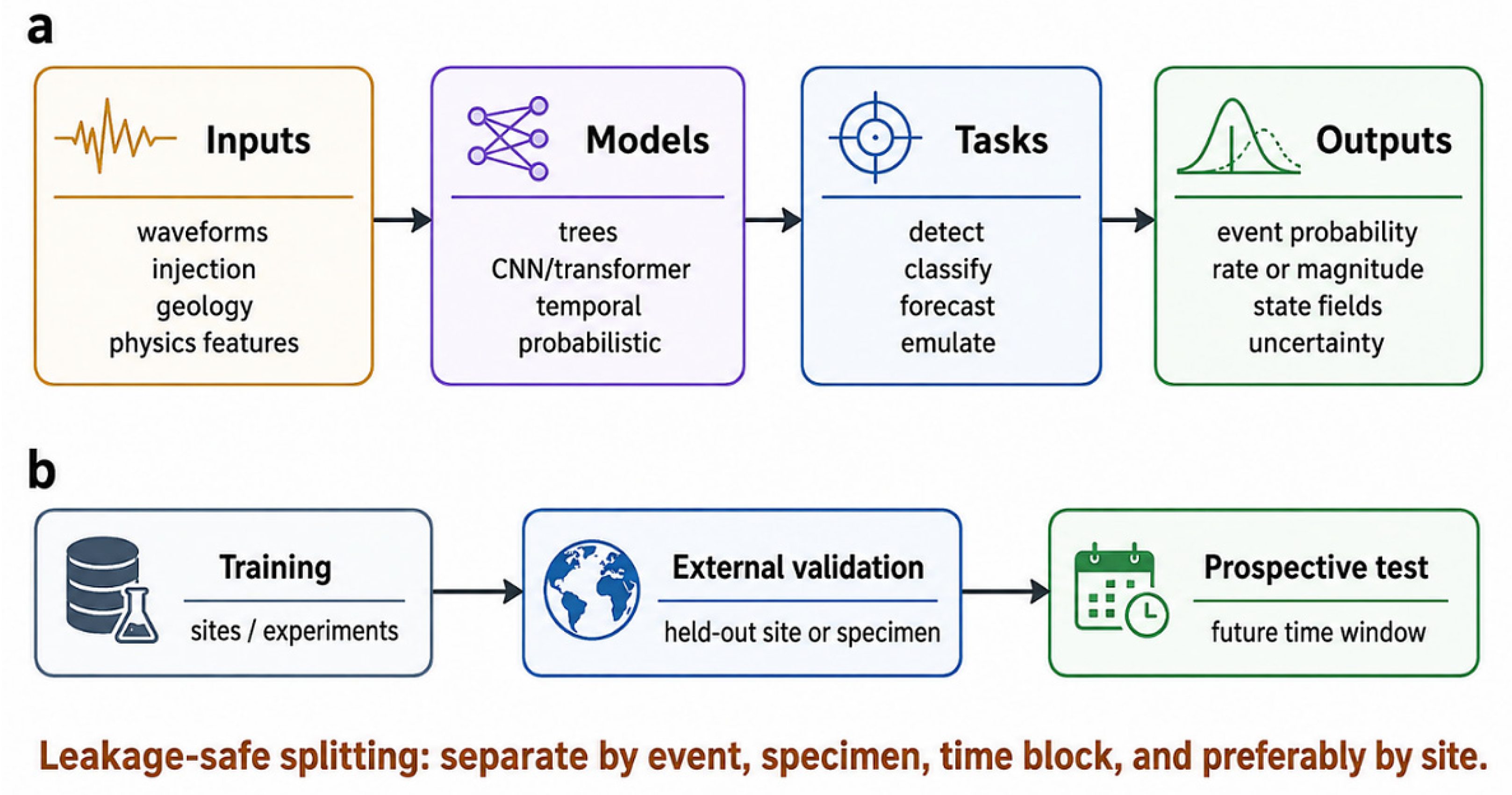
Figure 8.
Hybrid scientific machine learning architecture for fault reactivation assessment. A neural representation predicts state fields from coordinates and controls; physics residuals, monitoring observations, and training controls constrain the solution; risk metrics and uncertainty are derived from the predicted fields. Original synthesis based on Raissi et al. [26], Kadeethum et al. [90], Karniadakis et al. [14], Meguerdijian et al. [35], and Millevoi et al. [28].
Figure 8.
Hybrid scientific machine learning architecture for fault reactivation assessment. A neural representation predicts state fields from coordinates and controls; physics residuals, monitoring observations, and training controls constrain the solution; risk metrics and uncertainty are derived from the predicted fields. Original synthesis based on Raissi et al. [26], Kadeethum et al. [90], Karniadakis et al. [14], Meguerdijian et al. [35], and Millevoi et al. [28].
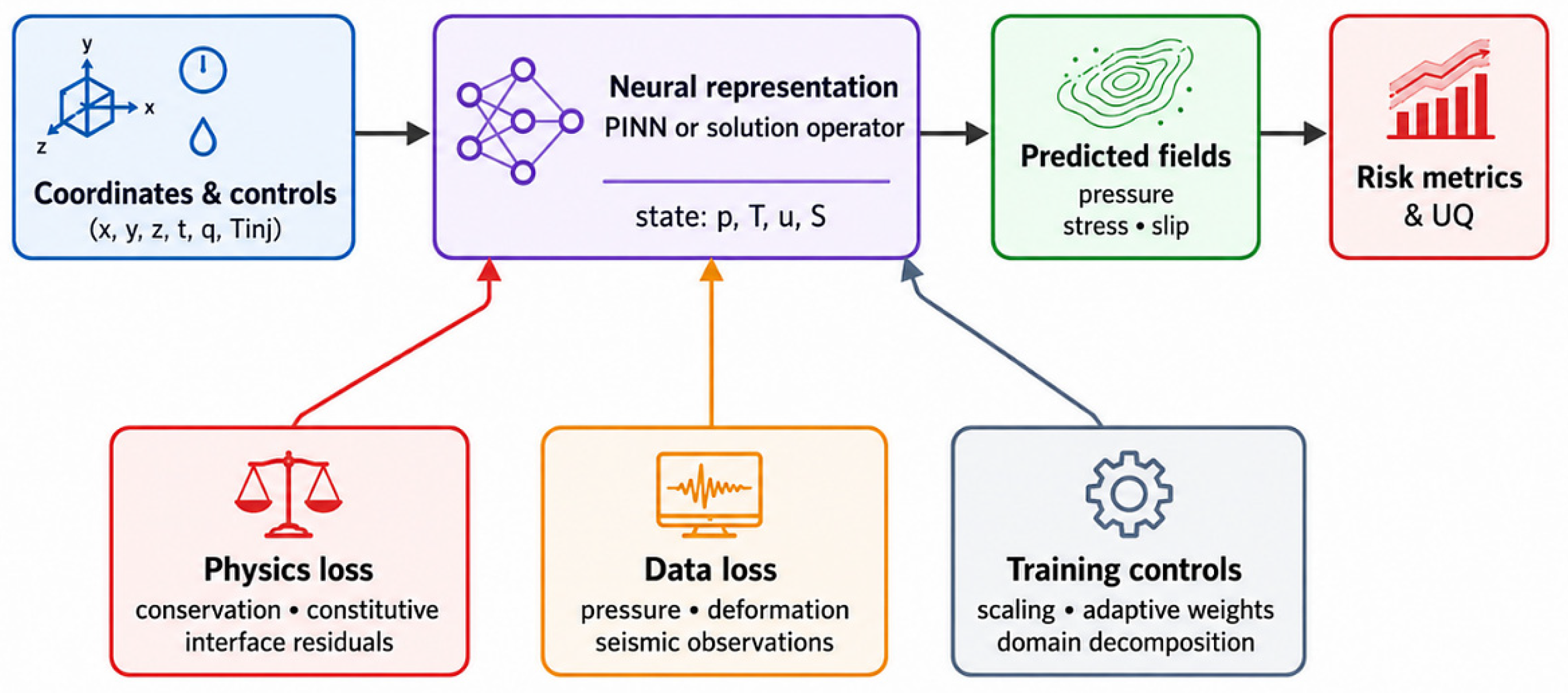
Figure 10.
Risk informed digital twin loop and aspirational research progression. Monitoring supports state updating; models forecast slip and containment risk; decision rules select rate, well allocation, or shut in options; and operations generate new observations. The timeline emphasizes open benchmarks and uncertainty standards in the near term, cross site validation and hybrid surrogates in the midterm, and auditable human supervised adaptive control as a condition for operational maturity. Original synthesis based on Mignan et al. [29], Karniadakis et al. [14], Vasylkivska et al. [30], and Willard et al. [27].
Figure 10.
Risk informed digital twin loop and aspirational research progression. Monitoring supports state updating; models forecast slip and containment risk; decision rules select rate, well allocation, or shut in options; and operations generate new observations. The timeline emphasizes open benchmarks and uncertainty standards in the near term, cross site validation and hybrid surrogates in the midterm, and auditable human supervised adaptive control as a condition for operational maturity. Original synthesis based on Mignan et al. [29], Karniadakis et al. [14], Vasylkivska et al. [30], and Willard et al. [27].
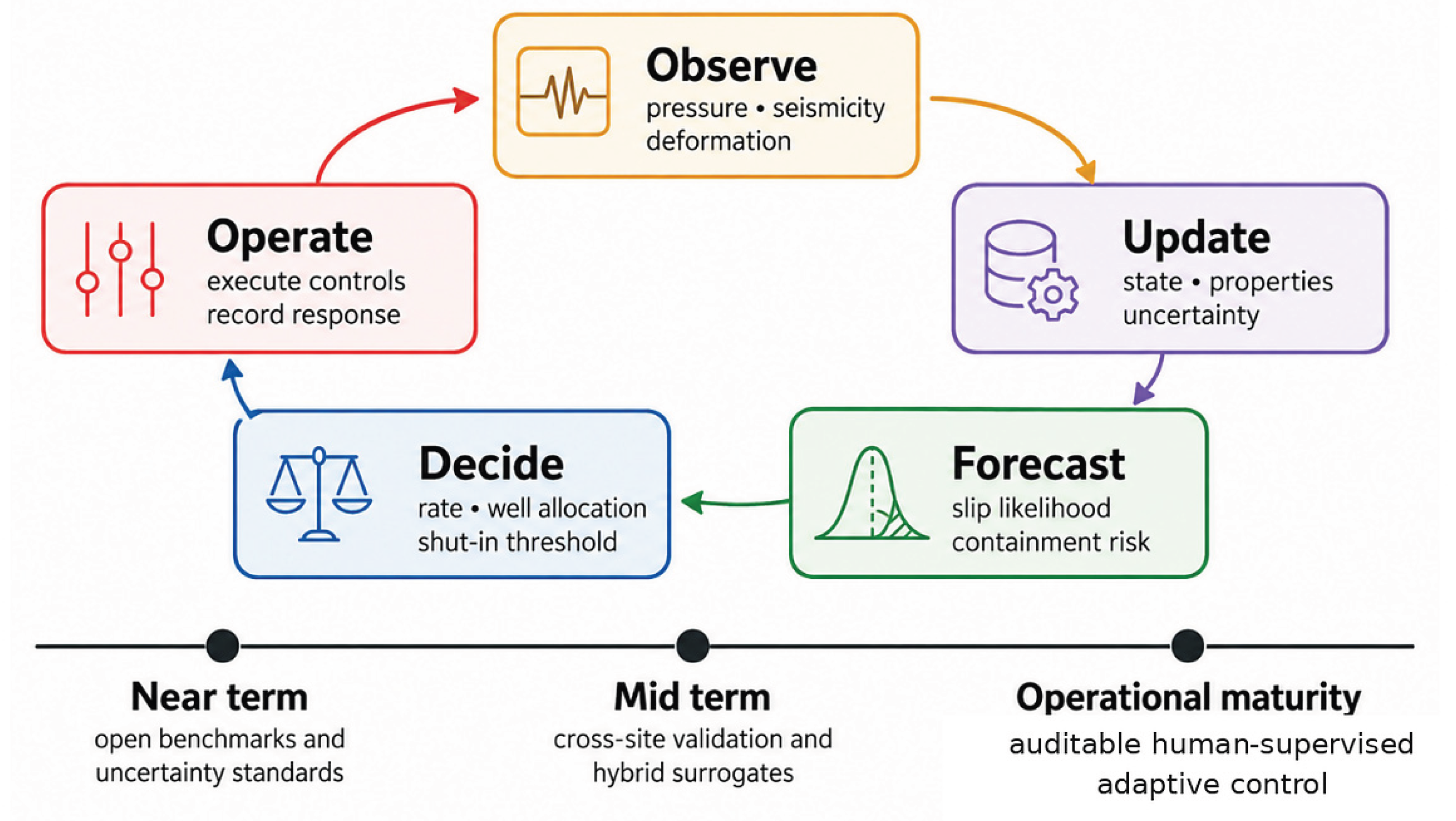

Table 1.
Structured critical review protocol and evidence coding.
| Review element | Protocol used in this review |
|---|---|
| Objective | Integrate multiphysics, monitoring, machine learning, and scientific machine learning around defined fault reactivation prediction targets and decision uses. |
| Sources | Scopus, Web of Science, Google Scholar, ScienceDirect, OnePetro, publisher databases, and backward/forward citation chaining. |
| Search coverage | Foundational literature through 10 August 2026; older studies retained when they establish governing theory, constitutive laws, numerical methods, or major field evidence. |
| Inclusion | Peer reviewed studies with clear relevance and sufficient information on geometry, physics, data, target, assumptions, or validation. |
| Exclusion | Duplicates, nontechnical commentary, insufficient methodological detail, and analogues without a clearly transferable mechanism or method. |
| Evidence setting | Direct CO₂ storage; controlled laboratory evidence; non CO₂ injection analogue; synthetic or numerical benchmark. |
| Validation level | Code verification; laboratory validation; retrospective field evaluation; cross site evaluation; prospective prediction. |
| Synthesis | Qualitative and mechanism based; no pooled performance statistic across noncommensurate targets and metrics. |
| Auditability | Search blocks, final update date, inclusion/exclusion logic, evidence categories, limitations, and source traceability are stated explicitly; no PRISMA compliant corpus is claimed. |
Table 2.
Prediction targets, observables, and appropriate evaluation metrics.
| Prediction target | Representative outputs | Required model elements | Relevant observations | Appropriate evaluation |
|---|---|---|---|---|
| Stability screening | Slip tendency, dilation tendency, ΔCFS | Stress tensor, fault attitude, pore pressure, friction | Stress tests, image logs, fault interpretation | Ranking stability; sensitivity; probability of threshold exceedance |
| First slip | Critical pressure, time, location | Pressure/stress evolution and yield criterion | Pressure, displacement onset, AE onset | Error in threshold/time/location with uncertainty |
| Slip evolution | Slip, slip rate, aperture, permeability | Post yield friction/damage law and feedback | Displacement, strain, AE, transmissivity | Time series error, energy consistency, hysteresis |
| Dynamic rupture | Rupture area, stress drop, seismic moment | Inertia, frictional weakening, wave radiation | Waveforms, focal mechanisms, spectra | Moment, source parameters, waveform or spectrum misfit |
| Seismicity forecast | Event probability/rate, magnitude distribution | Fault population and stochastic triggering law | Complete event catalogue and injection history | Log score, Brier score, information gain, calibration |
| Monitoring analytics | Detection, phase, class, location | Signal processing or ML model | Labeled waveforms with independent test data | Precision recall, false alarms, detection limit, location error |
| Containment consequence | Leakage rate, migration pathway, pressure relief | Multiphase fault flow and evolving transmissivity | Pressure, tracers, saturation imaging, geochemistry | Mass balance, breakthrough time, leakage probability |
Table 3.
Comparison of numerical formulations for fault reactivation problems.
| Formulation | Principal strengths | Principal limitations | Best supported use |
|---|---|---|---|
| Analytical / semi analytical | Transparent scaling; rapid screening; verification | Simple geometry and constitutive behavior | Pressure/stress bounds, slip tendency screening, code checks |
| Finite element | Complex geometry; contact; nonlinear mechanics; unstructured mesh | Multiphase flow may require specialized implementation; mesh dependence near faults | Site specific stress/deformation and interface mechanics |
| Finite volume / integrated finite difference | Local mass conservation; mature compositional multiphase flow; scalability | Complex fault mechanics often external or simplified | Regional plume and pressure evolution; coupled reservoir simulation |
| Explicit finite difference | Nonlinear geomechanics; large deformation; robust failure progression | Stability limited time step; structured geometry constraints | Quasi static field mechanics and selected dynamic problems |
| Block/particle DEM | Explicit discontinuities, opening, rotation, fracture creation | High cost; nonunique microparameter calibration | Laboratory scale failure, jointed rock, mapped fault networks |
| DFN continuum hybrid | Connectivity and pressure channeling; ensemble geometry | Sparse field constraints; coupling complexity | Fractured reservoirs and fault intersection sensitivity |
| XFEM / embedded interface | Nonconforming cracks and faults; reduced remeshing | Conditioning, integration, frictional contact, multiphase coupling | Crack growth or large fault sets in continuum models |
| Phase field | Natural nucleation, branching, and coalescence | Fine mesh; regularization dependence; difficult frictional flow | Process studies of tensile/mixed mode fracture |
Table 4.
Constitutive choices and the questions they can answer.
| Constitutive model | Represents | Can support | Cannot establish without extensions |
|---|---|---|---|
| Linear elasticity | Reversible stress and strain response | Poroelastic deformation and stress transfer | Irreversible slip, damage, permeability hysteresis |
| Mohr Coulomb / Drucker Prager | Pressure dependent yield and plastic flow | Onset and distribution of shear failure | Velocity dependence and dynamic nucleation |
| Cap plasticity | Compaction and pore collapse | Depleted reservoir compaction and stress paths | Discrete fault slip unless an interface is added |
| Constant Coulomb contact | Opening/closure and frictional sliding | Quasi static slip initiation and redistribution | Healing, velocity weakening, seismic/aseismic partition |
| Slip weakening | Friction drop with displacement | Dynamic rupture and stress drop | Time dependent healing unless added |
| Rate and state friction | Velocity and state evolution | Stable/unstable slip, nucleation, after injection response | Reliable field prediction without calibrated parameters and geometry |
| Damage / cohesive model | Progressive degradation and fracture energy | Crack initiation and growth | Mature fault friction after contact unless coupled |
| Permeability aperture law | Hydraulic feedback from deformation | Pressure redistribution and potential leakage | Multiphase fault flow unless capillary/relative permeability are included |
Table 5.
Field cases and their principal value for model evaluation.
| Case and evidence class | Injection setting | Key observations | Principal modeling value | Important limitation |
|---|---|---|---|---|
| In Salah, Algeria (direct CO₂ storage) | CO₂ storage in Krechba sandstone | Injection pressure, InSAR uplift, microseismic detections | Coupled pressure and deformation response; structural model updating | Limited seismic array and location resolution |
| Illinois Basin Decatur, USA (direct CO₂ storage) | CO₂ storage in Mt. Simon sandstone | Dense microseismic catalog, injection history, stratigraphy | Pressure diffusion, poroelastic stress transfer, statistical seismicity coupling | Basement fault properties and magnitude completeness uncertain |
| Otway, Australia (direct CO₂ storage) | Controlled saline and depleted reservoir tests | Active/passive seismic, fiber optics, pressure, plume monitoring | Monitoring design, small fault activation, model updating | Pilot scale; results are not directly scalable without modeling |
| Sleipner, Norway (contextual CO₂ storage) | Industrial offshore storage in Utsira Sand | Long term time lapse seismic, gravimetry, injection history, pressure response | Plume conformance, monitoring maturity, pressure/plume model evaluation | Limited direct evidence for fault slip or dynamic rupture |
| Snøhvit, Norway (contextual CO₂ storage) | Offshore injection in faulted Tubåen/Stø formations | Pressure increase, injectivity impairment, 4D seismic, reservoir switching | Operational pressure management; heterogeneity and compartmentalization | Not a prospective fault reactivation forecast test |
| Ketzin, Germany (contextual CO₂ storage) | Onshore saline aquifer pilot | Pressure, seismic, electrical, geochemical, and after injection monitoring | Integrated model updating, monitoring design, and closure evidence | Research scale and limited direct fault slip evidence |
| Basel, Switzerland (non CO₂ injection analogue) | EGS water stimulation in crystalline basement | High resolution seismic sequence including M≈3.4 | Traffic light systems, after injection response, maximum magnitude uncertainty | Not CO₂ storage; materially different geology and operations |
Table 6.
Evidence maturity of machine learning tasks relevant to fault reactivation assessment.
| Task | Direct CO₂ storage evidence | External or analogue evidence | Prospective validation and present maturity | Important limitation |
|---|---|---|---|---|
| Event detection and phase picking | Moderate; storage deployments exist but often require site specific adaptation | High in natural seismicity and geothermal monitoring | Some operational use; mature for catalog support after site validation | Domain shift across sites, sensors, and noise conditions; performance depends on network geometry and magnitude completeness |
| Waveform or source classification | Low to moderate; labels and storage specific datasets remain limited | Moderate to high in laboratory and tectonic datasets | Prospective storage validation is rare; emerging | Uncertain labels, class imbalance, and limited storage specific training data |
| Fault slip or no slip inference | Low; mainly simulation and limited laboratory transfer | Moderate in controlled friction experiments | Rare at field scale; research stage | Sparse positive field cases, scale transfer, and dependence on simulated or indirect labels |
| Seismicity rate or event probability forecasting | Low; few prospective storage tests | Moderate in EGS, disposal, and statistical seismology | Prospective skill remains largely unproven; research stage | Catalog incompleteness, nonstationarity, and very limited prospective field evaluation |
| Simulator surrogate or reduced order model | Moderate; mainly trained on synthetic/full order CO₂ ensembles | Moderate to high across subsurface simulation | Useful for bounded decision support; emerging to moderate maturity | Accuracy is bounded by the full order simulator and training design; threshold and outside domain errors may dominate |
| PINN based inverse estimation | Low; predominantly synthetic or benchmark evidence | Moderate for smooth PDE inverse problems | Rare cross site or prospective validation; research stage | Optimization instability, parameter nonuniqueness, discontinuities, and governing model error |
| Neural operator field prediction | Low to moderate; growing CO₂ flow demonstrations | Moderate in parametric PDE benchmarks | Fast inference is demonstrated, but field transfer remains emerging | Geometry and domain shift, conservation error, and unreliable extrapolation beyond the training distribution |
Table 7.
Machine learning tasks, validation units, and preferred metrics.
| Task | Sampling unit that must be separated | Main metrics | Frequent failure mode |
|---|---|---|---|
| Event detection | Continuous time block and event | Precision recall, false alarms/time, detection probability vs magnitude/SNR | Random windows from same event in train and test |
| Phase picking | Event/station/site | Pick error distribution, missed picks, outliers | Evaluating only high SNR curated events |
| Waveform classification | Event/specimen/experiment | Class precision/recall, calibration, confusion matrix | Uncertain labels and duplicate augmented traces |
| Source location | Event and array geometry | 3D error volume, coverage of uncertainty region | Reporting distance to one preferred hypocenter only |
| Slip/no slip classification | Experiment, time block, site | PR AUC, Brier score, recall at specified false alarm rate | Severe class imbalance hidden by accuracy |
| Seismicity rate forecast | Future time window and spatial cell | Log score, information gain, count deviance, calibration | Temporal leakage and MAPE near zero counts |
| Simulator surrogate | Geological realization and scenario | Field error, mass balance, threshold error, uncertainty coverage | Random cell wise split and extrapolation beyond design |
Table 8.
Minimum model credibility reporting checklist.
| Domain | Minimum reporting items |
|---|---|
| Objective | Prediction target, spatial/temporal domain, decision use, unacceptable outcomes |
| Geometry | Stratigraphy, fault interpretation, alternative structural models, mesh/grid resolution |
| Initial state | Stress tensor and uncertainty, pressure, temperature, saturation, depletion history |
| Physics | Governing equations, phase behavior, capillary/relative permeability, thermal and chemical assumptions |
| Constitutive behavior | Elastic/plastic parameters, fault friction, dilation, aperture/permeability laws, calibration range |
| Coupling | One way, staggered, or monolithic scheme; exchanged variables; convergence tolerance |
| Verification | Benchmarks, mass/energy balance, mesh/time step convergence, solver residuals |
| Calibration | Data used, parameters adjusted, objective function, posterior correlation/nonuniqueness |
| Validation | Independent data, observation operator, error model, detection limit, prospective status |
| Uncertainty | Parameter ranges/distributions, structural alternatives, model discrepancy, surrogate error |
| Reproducibility | Software/version, scripts, input files, random seeds, data availability, hardware where relevant |
| Decision governance | Thresholds, abstention/outside domain rule, human oversight, audit trail |
Table 9.
Priority research needs and evidence required for progress.
| Priority | Near term deliverable | Evidence required before operational use |
|---|---|---|
| Stress and fault characterization | Ensemble 3D structural/stress models | Reconciliation with well, seismic, and deformation observations |
| CO₂ conditioned fault friction | Shared rate and state, dilation, and permeability datasets | Independent laboratories and multiple rock/gouge types |
| THMC fault flow coupling | Calibrated reaction and property relations | Long duration mechanical and flow validation |
| Open benchmarks | Verified synthetic and laboratory cases | Public inputs, outputs, metrics, and reference solutions |
| Cross site ML validation | Common event and forecast tasks | Held out sites, calibrated probabilities, detection limits |
| Fault aware PINNs/operators | Interface capable architectures | Conservation, threshold, and outside domain tests |
| Surrogate uncertainty | Error aware probabilistic emulators | Coverage tests against full order and field data |
| Digital twin governance | Auditable model/data/control architecture | Prospective pilots with human oversight and fallback rules |
Disclaimer/Publisher’s Note: The statements, opinions and data contained in all publications are solely those of the individual author(s) and contributor(s) and not of MDPI and/or the editor(s). MDPI and/or the editor(s) disclaim responsibility for any injury to people or property resulting from any ideas, methods, instructions or products referred to in the content. |
© 2026 by the authors. Licensee MDPI, Basel, Switzerland. This article is an open access article distributed under the terms and conditions of the Creative Commons Attribution (CC BY) license (http://creativecommons.org/licenses/by/4.0/).
Copyright: This open access article is published under a Creative Commons CC BY 4.0 license, which permit the free download, distribution, and reuse, provided that the author and preprint are cited in any reuse.


