

Submitted:
08 August 2026
Posted:
14 August 2026
You are already at the latest version
Abstract
We propose a non-Lambda-CDM framework, Multi-tier Newtonian Gravity (MULTING), that builds cosmic expansion history from local, pairwise gravitational interactions between cosmic-web nodes, rather than assuming a single global metric from the outset. We hypothesize that a node’s intracluster medium (ICM) thermal energy induces a repulsive, dipole-like gravitational force component, motivating a multipole expansion of the two-body force law between nodes. By fitting 33 data points (31 Cosmic Chronometer H(z) measurements (0<z<1.97), SH0ES, and a DESI DR2 Lyman-alpha measurement at z=2.33), MULTING produces a well-identified solution family that reduces the Planck-SH0ES tension, while performing as well as or somewhat better than flat Lambda-CDM, fixed at its standard published values, on both chi-squared and Pearson-r across all 33 points.
Keywords:
Hubble tension
; rate of expansion of the universe
; galaxy clusters
; intracluster medium
; dark energy
; gravitational multipole moments
; gravity
; MULTING
1. Introduction
The Hubble tension represents a major challenge [1,2] within the study of cosmology. The Hubble tension features gaps between data about the Hubble parameter and results that CDM modeling produces. CDM modeling links the Hubble parameter and the rate of expansion of the universe.
In this paper, we suggest modeling that fits Hubble parameter data comparably to, and within a specific, clearly-bounded redshift range marginally better than, CDM modeling that has bases in the Friedman-Lemaitre-Robertson-Walker (FLRW) metric [3,4]. That CDM modeling links to the notion of dark energy [5,6].
Table 1 summarizes aspects regarding two known eras in the rate of expansion of the universe and one possibly impending era in the rate of expansion of the universe. (See Sec. Section 4.1 for context and references regarding Table 1.) We note here, as an aside, that Section 4.17 examines the possibly-impending era and discusses a related, distinct transition that our work finds instead.
CDM FLRW modeling tries to explain the known eras via structural aspects of space-time. (See Section 4.2 for information about CDM FLRW modeling regarding the rate of expansion of the universe.)
In standard physical cosmology, including the CDM paradigm, a direct and mathematically exact mapping links the global, isotropic expansion rate of the space-time metric to the physical separation rate of structural nodes within the cosmic web [3]. At large scales (, with Mpc denoting megaparsecs), this relationship is governed strictly by the Hubble-Lemaitre Law, wherein the physical distance vector between distinct nodes evolves proportionally with the cosmic scale factor via , where x is the comoving coordinate spatial vector mapping the fixed grid positions of the structural nodes, independent of the expanding cosmic scale factor. Differentiating this relation yields a relative kinematic separation velocity driven entirely by the Hubble parameter, , an observational expansion vector directly constrained across cosmic time by differential-aging cosmic chronometer vectors [7]. While standard linear perturbation theory treats the separation of these virialized nodes as a passive consequence of a homogeneous background fluid, modern macroscopic gravity frameworks and cosmological averaging protocols demonstrate that the non-linear growth, spatial distribution, and localized dynamics of these massive nodes are coupled bottom-up to the global evolution of [8]. Consequently, modeling the localized, pairwise dynamical interactions between nodes might provide an empirically grounded baseline for tracking macroscopic cosmic expansion.
The 31 Cosmic Chronometer data points [9,10,11] (which span the range ) are, individually, far noisier in relative terms than either the SH0ES local distance-ladder measurement ( km/s/Mpc at [1]) or the independent DESI DR2 Lyman- measurement at ( km/s/Mpc [12]). Our framework treats SH0ES and DESI as data points, each carrying its own tight (compared to the 31 Cosmic Chronometer points) uncertainty, alongside the 31 Cosmic Chronometer points, and jointly optimizes all three free parameters, unconstrained, against the resulting 33-point ensemble. This yields a well-identified family of solutions (Section 3), spanning the real, Planck-SH0ES tension, that outperforms flat CDM, fixed at its standard, published values -- the matter density and dark-energy density , each expressed as a fraction of the total energy density that sets the universe’s expansion rate -- on both and Pearson-r across nearly the entire range. The unconstrained optimum -- the spotlighted case, with the lowest of any configuration we tested -- is this paper’s primary result. (The subscript 33 in denotes the number, 33, of data points.) We additionally feature a second, SH0ES-anchored comparison case, fixed to hit SH0ES’s value exactly, because it permits the most direct, apples-to-apples test in this paper. Against flat CDM required to hit the identical value ( fixed, optimized), MULTING’s SH0ES-anchored case still comes out narrowly ahead on both measures. Both results rest on, and do not erase, the following underlying fragility, discussed in depth in Section 4.11 and Section 4.13: Fit to the Cosmic Chronometer data alone, without SH0ES or DESI included directly, our framework exhibits a near-total cancellation between two force terms that leaves it fragile under extrapolation. Section 3 reports both cases in full. (See Section 4.3 for information about the Hubble tension and some other gaps between data and CDM modeling.)
2. Methods
The Multi-tier Newtonian Gravity (MULTING) framework models cosmic expansion not as a global space-time metric expansion, but as a bottom-up, macroscopic phenomenological force law governing the relative kinematics of localized cosmic-web nodes. (See Section 4.4 for a table that lists similarities and differences between MULTING and CDM.)
We explore explaining the known eras in the rate of expansion via the mechanisms that govern gravitational interactions between neighboring nodes. Each node exists where two or more filaments overlap. Each node includes one galaxy cluster or a few galaxy clusters.
2.1. Theoretical Framework: Macroscopic Force Formulation
We suggest a theoretical framework: multi-tier Newtonian gravity (MULTING). We define tiers as successive terms in a multipole-like expansion of gravitational interactions. This tier structure was originally motivated by the hypothesis that each tier would dominate its own era of cosmic history: the quadrupole tier, featuring mutual attraction between nodes, motivating the first era that Table 1 lists; the dipole tier, featuring mutual repulsion between nodes, motivating the second era that Table 1 lists; and the monopole tier, featuring mutual attraction between nodes, motivating the possible third era that Table 1 lists. Fitting this framework to SH0ES, Cosmic Chronometer, and DESI data (Section 2.7) shows that quadrupole and dipole couplings are necessary to reproduce the observed expansion history, but does not show each tier cleanly dominating a temporally-segregated era in the way originally hypothesized. (See Section 3 for detailed discussion.) We therefore present the tier structure below as the motivating hypothesis for this framework’s functional form, not as an already-established temporal correspondence. (See Section 4.5 for information about uses of the word multing.)
Regarding nodes, cosmology measures the properties mass, radius, thermal energy, and bulk energy (as in the energy that characterizes bulk motions within the node). The thermal energy is the total of the kinetic energies of the nucleons and electrons that comprise the intracluster medium (ICM) of a node. Except for during relatively rare and relatively brief mergers, within nodes, of galaxy clusters, about 70 percent to 90 percent of a node’s ICM kinetic energy is thermal energy [13,14,15]. We suggest that thermal energy is an aspect of a gravitational property that provides a basis for a gravitational force component that is spatially dipole with respect to distance away from a node and is isotropic with respect to angle. (See Section 4.6 for the physical motivation, and (drawn in part from an analogy with electromagnetism) for why thermal rather than bulk kinetic energy is treated as the basis for this dipole component.)
MULTING suggests that Eqs. (1) through (4) pertain for gravitational effects of a node-A on a node-P. The forces , , , and align with the spatial vector from node-A to node-P, with negative contributions to providing attraction of node-P toward node-A and positive contributions to providing repulsion of node-P away from node-A. The superscripts , , and associate respectively with the words monopole, dipole, and quadrupole, following the standard convention for orders in a multipole expansion. Newtonian gravity [16] includes Eq. (2) and does not include Eqs. (3) and (4). s is the length of a vector that extends from the position of node-A to the position of node-P. G is the gravitational constant. is the mass of node-A. Masses are nonnegative. is the mass of node-P. is a length that associates with a notion of a radius of node-A. is a length that associates with a notion of a radius of node-P. is the thermal energy that associates with the ICM of node-A. is nonnegative. has dimensions of mass. is the thermal energy that associates with the ICM of node-P. is nonnegative. has dimensions of mass. is a positive number that we suggest might be approximately independent of the choice of a specific node; the subscript 1 in corresponds to the dipole order, , in . is a positive number that we suggest might be approximately independent of the choice of a specific pair of nodes; the subscript 2 in corresponds to the quadrupole order, , in .
2.2. Theoretical Framework: Kinematic Effects Formulation
Newtonian physics suggests that Eq. (5), the general form of Newton’s second law for a system of time-varying mass [17], pertains regarding the motion of node-P. denotes the velocity of node-P. t denotes cosmic time.
Regarding our work, we suggest that Eq. (5) represents a special case in which matter joins node-P with zero velocity, measured in the same reference frame as . Eq. (6) is the general, momentum-conserving form. denotes the velocity of the matter joining node-P at the instant of accretion. Eq. (5) is the special case .
For the two-node system of Section 2.1, each node has its own, in general independent, accretion history. Combining Eq. (6) for both nodes and forming the reduced-mass equation for the node-pair separation s yields Eq. (7), where is the reduced mass of the node pair. (See Section 4.7 for the specific treatment adopted for the bracketed term ( isotropic-versus-merger-driven accretion) and the inputs used to constrain it.) The symbol ˙ (or one overdot) denotes the first derivative with respect to time t. The symbol ¨ (or two overdots) denotes the second derivative with respect to time t.
2.3. Kinematic Translation Protocol
To map these localized, pairwise node interactions to the macroscopic evolution of the universe, we implement a kinematic translation protocol. We define the scale factor , the same scale factor introduced in standard FLRW cosmology (Section 4.2); we use as a bridging device to connect this framework’s local dynamics to the observational, redshift-based quantities discussed there, not as an assumption this framework otherwise relies on. We let denote the characteristic distance between adjacent cosmic-web nodes at redshift z. The pairwise relative acceleration between nodes, , is mapped directly to the cosmic scale factor acceleration via Eq. (8). The overdots denote differentiation with respect to cosmic time t.
To transition from temporal kinematics to the observational domain, we apply the standard differential mapping [3,4], which links the time-evolution of the scale factor to the redshift integration space.
Integrating , using the relative acceleration of Eq. (8), with respect to redshift yields ; taking the square root gives the dynamic Hubble parameter . This bottom-up approach bypasses the fluid-homogeneity assumptions of the standard Friedmann-Lemaitre-Robertson-Walker (FLRW) metric, treating the background expansion as an integrated average of discrete node dynamics. We call this integration constant , since its value is imposed at a chosen reference redshift rather than derived independently -- the same role plays in the standard FLRW construction, adapted here to this framework’s own derivation. One clarification worth stating explicitly, for a reader reconstructing itself rather than only : is not an incomplete initial condition for the second-order equation governing ; it is the single combination, , that the trajectory alone depends on. Recovering itself requires both and separately; these are given by Mpc (Section 2.4) and , not by any separate, independently-fitted quantity.
2.4. Analytical Formulation: Empirical Scaling Laws
This subsection derives each node property’s redshift evolution in turn: mass (theoretical), radius (derived from mass via critical density — the framework’s most significant residual circularity), and temperature, gas mass, and thermal energy (the latter two grounded in real X-ray data). Readers mainly interested in results rather than derivation may wish to skip ahead to Section 3.
In plain terms: every quantity derived below is an ingredient that gets plugged into -like considerations for a single pair of nodes at a given redshift -- mass and radius set the gravitational force and its multipole corrections, thermal energy sets the dipole and quadrupole terms, and separation converts force into the acceleration, , that ultimately builds . Nothing here requires cosmology beyond this.
The physical properties of the nodes are not static; they evolve across cosmic time due to hierarchical structure growth. For X being either A or P, we model node mass using an empirical power law [18,19] relative to a low-redshift baseline .
Effective radius and ICM thermal energy are each derived from rather than assigned independent power laws, for reasons given below. (See Section 2.6 for the classification (data-proximate / retained-theoretical / circular) of each input below.)
Radius is derived, not given an independent exponent: -type radii are conventionally defined via mass and the critical density [15], , not measured independently, so we adopt
where is the same relation evaluated at , is the node mass baseline of Eq. (10), and (flat CDM, ) [2]. This follows directly from , . We flag this explicitly as the most significant residual FLRW-dependence in this framework: it assumes the Friedmann equation to construct an input that then feeds the force law whose purpose is to independently predict . (See Section 2.6 for why this is not resolvable simply by sourcing additional data.)
We build , the ICM thermal energy used in the force law of Section 2.1, through three steps: a theoretical mass-to-temperature scaling, a data-fitted temperature-to-gas-mass relation, and a direct combination of the two into an energy. Only the first step is purely theoretical; the second is grounded in real X-ray data; the third is definitional.
Step one: mass to temperature. Clusters of different mass are assumed to be scaled versions of one another -- a “self-similar” scaling, in the standard astrophysical sense [20]: a single power-law relation connects mass to characteristic temperature, , with no free parameters beyond the overall normalization. We report in keV, following the standard astrophysical convention of quoting (Boltzmann’s constant times temperature, an energy) rather than temperature itself in Kelvin; this is an intensive, per-particle energy scale, distinct from the extensive, total ICM thermal energy this subsection is building toward. The two are related directly, not independently specified: step three below obtains from by multiplying by the total number of ICM particles.
with keV. This value is recalibrated, not an independent theoretical guess: an earlier value ( keV) produced gas fractions of 0.35–0.37 when carried through the gas-mass step below — roughly 2.5x the realistic range for massive clusters (~0.10–0.15, below the cosmic baryon fraction) [21]. keV is chosen so that the implied gas fraction is 0.13 at , which keeps the gas fraction in a realistic 0.118–0.127 range across the full cosmic-chronometer redshift span used in this work (checked directly, not only at ). This recalibration surfaces, rather than resolves, a further tension: it implies cluster temperatures of only – keV across this range for –, noticeably below the keV independent, weak-lensing-calibrated mass-temperature scaling relations would suggest for that mass [22]. There is no single that simultaneously satisfies realistic gas fractions and realistic mass-temperature normalization here, because itself remains a theoretical, not data-grounded, input (see Section 2.6).
Step two: temperature to gas mass. Unlike step one, this step is a direct fit to real X-ray data, not a theoretical scaling:
with keV, , and the pivot temperature, gas mass, and redshift of the fit below, chosen (by that fit’s own authors) to minimize correlation between the fitted slope and normalization; and are that fit’s empirical mass-temperature slope and redshift-evolution exponent, respectively, a fitted –T relation from the largest cluster X-ray sample to date (3061 clusters, ) [23]. A weak-lensing-calibrated alternative for this step was considered and deliberately not adopted (see Section 2.6 for why).
Step three: combining into an energy. The total ICM thermal energy is, by definition, the number of ICM particles times their mean thermal energy:
with the mean molecular weight (distinguished from the reduced mass of Section 2.2) and the proton mass (distinguished from , the mass of node-P).
2.5. Analytical Formulation: The Kinematic Side of the Equation of Motion - Non-Isotropic Mass Accretion
This subsection derives the non-isotropic mass-accretion correction to the two-body equation of motion — the term accounting for merging substructure carrying its own momentum. The key results — the coherence and merger fractions, and the resulting correction’s role in the fit — are summarized without derivation in Section 2.7.
In plain terms: assumes constant mass. A node gaining mass by accretion is more like a rocket gaining fuel mass in reverse -- incoming material carries its own momentum, which must be accounted for directly, not folded into a as if mass were fixed. This subsection derives that correction.
For an identical “typical node” case we adopt for computational purposes (, , ), we adopt the following treatment of the bracketed term in Eq. (7), built from three citable inputs and one explicitly-flagged modeling assumption:
, a characteristic merger infall velocity, defined self-consistently via
i.e. the standard circular-velocity formula, , borrowed here purely as a characteristic velocity scale for a typical node -- not implying that a node is in literal circular orbital motion -- consistent with cluster-merger infall speeds of order 1000–1200 km/s reported for massive clusters from an analytic turnaround-radius estimate [26], cosmological N-body estimates for typical CDM cluster mergers [27], and a directly observed massive cluster merger [28];
, the fraction of a node’s merger-driven momentum flux that we suggest projects coherently onto the axis connecting a given node pair, rather than being isotropically distributed among the several filaments that meet at a node. We bound, rather than derive, using observed and simulated cosmic-web connectivity statistics: nodes of cluster mass typically connect to filaments [29,30], so that under the simplest possible assumption (accretion divided evenly among a node’s filaments). We adopt () as an illustrative, literature-bounded value; we emphasize that is a stated modeling assumption, not a measured quantity, and that a dedicated exploration of its plausible range is left to future work.
We define the coherent velocity mismatch,
and the resulting accretion-correction force,
where follows directly from Eq. (10) via . We take to act with the same sign as and (i.e., opposing net repulsion), consistent with the general character of variable-mass mechanics: growing mass by incorporating matter of differing velocity generically resists acceleration, in the same manner as the classical growing-raindrop or snowplow problem. We flag explicitly that this sign, like , is a first-pass modeling choice for this specific two-node geometry and has not been independently derived from first principles.
The kinematic translation protocol of Section 2.3 is modified accordingly: Eq. (8) is evaluated using in place of alone.
2.6. Analytical Formulation: Empirical Grounding of the Model’s Inputs, and of Evidence More Generally
Because MULTING aims to depend on measured data as much as reasonably possible, rather than on the FLRW/CDM framework that it is proposed as an alternative to, it is useful to state plainly how directly each input to Eqs. (10) through (14) is grounded in observation, as opposed to grounded in theoretical assumptions that themselves presuppose the standard cosmological model. We offer the classification below not only as an audit of MULTING’s own inputs, but as a general, transferable tool: given that CDM has been the dominant paradigm guiding cosmological research for roughly three decades, it is reasonable to ask, for any dataset or derived quantity used in this field, to what extent that paradigm shaped not only how the quantity was calibrated, but how it was sought out, obtained, and interpreted in the first place. We classify each input into one of three classes, avoiding the word “tier” for this classification to prevent confusion with the multipole tiers (monopole, dipole, quadrupole) that structure Eq. (1).
In plain terms: does not care where F, m, and a come from, but trusting the equation’s output means trusting its inputs. The classification below is simply an accounting of which inputs are close to direct measurement and which rest on theoretical assumption, for a reader who wants to know how much of this framework’s output is data and how much is inherited structure.
Class I, data-proximate: an input whose only dependence on the standard cosmological model is the essentially unavoidable use of a fixed, external (“fiducial”) cosmology to convert a survey’s raw observables (flux, angular size, weak-lensing shear) into physical units. This dependence does not assert what MULTING’s own dynamics should produce; it is shared by essentially every astronomical catalog in existence, and is not a circularity specific to this framework. The 31-point cosmic chronometer compilation used to test this framework falls in this class, since differential galaxy ages are inferred from stellar population synthesis rather than from an assumed expansion history. ICM thermal energy, , can likewise be placed in this class if grounded in directly measured cluster X-ray scaling relations [23] rather than left as the purely theoretical self-similar assumption of Eq. (14). This grounding has a limit worth stating precisely: the underlying catalog covers [23]. Six of the 31 Cosmic Chronometer data points used throughout this paper lie beyond it, so this framework already extrapolates its one directly data-grounded input for part of its own calibration range. The theoretical mass-evolution law of Eq. (10) rests on halo merger-rate simulations covering a considerably wider range, [18], but our own fixed exponent is a simplification of that simulation’s own results, and a single exponent is unlikely to track hierarchical growth accurately across so wide a span even where the underlying simulation data remains good. Taken together, we regard as the most defensible boundary of data-grounded territory in this framework, as one further, uncomfortable but not unreasonable extrapolation, and results reported for as resting on assumptions this paper cannot currently support directly. One specific exception is deliberate, not an oversight: we do extrapolate this framework’s theoretical inputs out to DESI’s point, precisely in order to test the model against a real, independent measurement beyond the rigorous boundary. We regard this as a stress test of the model, not a claim that predictions at generally are well-supported.
Class II, retained-theoretical: an FLRW-flavored theoretical step, kept deliberately after checking whether a more directly empirical alternative is actually less model-dependent. The node mass evolution law, (Eq. (10)) [18,19] falls in this class, as does the inter-node separation law of Section 2.3, which is notable for invoking no assumed background expansion-rate function at all — the least FLRW-flavored input in this framework, even though it remains a theoretical assumption rather than a directly measured relation. We also considered, and deliberately did not adopt, a weak-lensing-calibrated mass–temperature relation [22] as a substitute for the self-similar mass-temperature step used in our computations: such relations are constructed via likelihoods evaluated at a fixed cosmology, with the matter density varied using external supernova priors, making them more deeply cosmology-dependent, not less, than the simple theoretical assumption retained here. This illustrates a general point: substituting a more directly empirical relation does not always reduce a model’s dependence on the standard cosmology, since the empirical relation’s own construction may itself lean more heavily on that cosmology than the theoretical shortcut it replaces.
Class III, circular: the input is constructed by assuming the very relation — here, the Friedmann equation — that the model aims to test independently. This applies to the node radius, , when constructed via the standard -type definition, in which radius is set by an assumed critical-density evolution, , . This directly assumes the Friedmann equation to build an input that then feeds the very force law whose purpose is to independently predict . We flag this as the most serious residual dependence in the present computations, the same species of circularity that motivates cosmological averaging and back-reaction concerns more generally [8,31]. (See also Section 4.15.) It is not resolvable simply by sourcing additional data, since the definition, as used field-wide, already carries this assumption at the point of measurement; any cluster catalog’s reported radii inherit it.
The three classes above address calibration — the conversion of raw observables into physical units and derived quantities — but a fuller assessment of CDM’s influence extends further, into how evidence is sought, obtained, and reported. For example, cluster evolution is conventionally reported using the self-similar basis function rather than a model-agnostic functional form; this is a reporting convention, not a strict requirement of the underlying X-ray or lensing measurement, and it can make departures from CDM-consistent evolution harder to notice or communicate than they might be under a differently parameterized report. Similarly, survey design — which redshift ranges, halo masses, or sky regions receive deep follow-up — and the scrutiny an anomalous result receives can both be shaped by expectations set by the dominant paradigm, independent of any single calibration step. We do not attempt a comprehensive audit of these effects here; we note them explicitly so that the three-class framework above is understood as a partial, not complete, accounting of CDM’s influence on the evidence base this and other papers draw upon.
We further note that this classification is not specific to MULTING, nor does it presuppose that CDM’s own observational pipelines are exempt from it. Baryon acoustic oscillation analyses, Type Ia supernova standardization, and weak-lensing shear calibration each involve their own chains of assumed-cosmology-dependent reduction steps, of varying depth, that a reader could in principle subject to the same three-class assessment, and to the broader seeking/reporting considerations of the preceding paragraph. Undertaking that assessment for CDM’s own evidentiary base is outside the scope of this paper. We offer the classification here, in the hope that it — or an improved version of it — might be applied symmetrically, as a small contribution toward helping readers judge, for any specific claim in this field, how much of its evidentiary support is independent of the paradigm under test.
Finally, we emphasize that this classification is intended as a plain, direct accounting, and as a starting point for a broader, symmetric practice, not as a claim that full independence from CDM is achievable, by MULTING or by any other framework. Redshift itself, and virtually all astronomical unit calibration, already presuppose cosmic expansion at some level; our aim is to minimize and make explicit the model’s dependence on the specific FLRW dynamical relations it is proposed as an alternative to, and to invite the same scrutiny of the evidence base more broadly, not to claim a dependence-free derivation.
2.7. Computational Details
The framework has three free parameters: the two couplings and , and a local Hubble-parameter anchor, . These are determined by chi-squared minimization of the integrated curve (Section 2.3) against the 31 Cosmic Chronometer data points, the SH0ES point, and the DESI point (33 total), subject only to , , and the numerical requirement (i.e., the squared value of H at , not H evaluated at ), where is the n-th of the 33 redshifts, at every fitted node. No requirement is imposed on which force term dominates at any specific redshift, before or during optimization. The tier-and-multipole structure of Section 2.1 is treated as the motivating hypothesis for this framework’s functional form, not as a fitting constraint to be enforced or tested at specific redshifts. (See Section 4.11 for why.) In addition to this free-floating fit, we also fix at several representative values, including the SH0ES local distance-ladder value, re-optimizing only and against each; and we separately fit against only the subset of data points for which the underlying relation is directly data-grounded, evaluating the resulting fit against the remainder.
Optimization uses a multi-start Nelder-Mead search [32] from several generic starting points spanning several orders of magnitude in and , chosen without reference to any physically-motivated threshold, with the best feasible result retained across starts. As a safeguard, if no start converges to a feasible point, a bounded differential-evolution fallback would be used, with bounds wide enough to include the largest coupling values found in any run to date, plus a two-order-of-magnitude margin; this fallback was not needed for any result reported in this paper.
Goodness of fit is reported via and the Pearson correlation coefficient, computed identically for this framework and for a flat CDM curve fit directly to the same 33 points, so that the comparison is fair. We do not report the Akaike or Bayesian Information Criteria (AIC, BIC) in this paper: a parameter-count penalty presupposes that the compared models’ structures were fixed independently of the data under test, an assumption that holds far more securely for CDM, given its long, independently-cross-validated history, than for a framework still in active development. (See Section 4.9 for more discussion.)
Two diagnostics are reported for the fitted model. Eq. (18) shows one diagnostic, the deceleration parameter [3,4].
The other diagnostic is the individual force-term decomposition (, , , and the accretion correction of Section 2.5).
is reported for comparability with the standard cosmology literature. The force-term decomposition is the primary diagnostic of this framework’s own behavior (See Section 4.11 for the decomposition itself, quantified, and why this distinction matters.)
3. Results
This section reports some of our framework’s key results.
Three types of measurements ground the results: the 31-point Cosmic Chronometer compilation of Section 2.7, the SH0ES local distance-ladder measurement ( km/s/Mpc [1]), and the DESI DR2 Lyman- baryon acoustic oscillation measurement at its reported effective redshift, ( km/s/Mpc [12]), itself drawn from an underlying Lyman- forest and quasar sample spanning -- unlike SH0ES, this measurement has a single, directly-computed effective redshift (Section 4.12).
Rather than fix an exactly at SH0ES, we treat SH0ES and DESI as data points, each carrying its own comparatively tight uncertainty, alongside the 31 Cosmic Chronometer points, for 33 points in total, and jointly optimize all three free parameters (, , and ) against all 33 data points simultaneously. This lets the fit itself determine how much of the Hubble tension to close, rather than presupposing a full or zero resolution, and lets us ask directly: across the resulting range of possible tension reductions, does this framework remain competitive with, or outperform, flat CDM fixed at its standard, published values (, [2])?
Table 2 lists values of and reports optimized and at each value. ([33] discusses calculations that produce information that Table 2 reports.)
Two flat CDM benchmarks, computed over the same 33 points, put this table’s numbers in context.
The first is extant CDM, fixed at its standard, published values (, [2]), not re-optimized in any way: , .
Five of the table’s seven rows outperform the first benchmark on . The last two rows ( and ) fall short of it, since matching closer to Planck costs more, in fit quality to the other 32 points, than it gains. On Pearson-r, every row outperforms the first benchmark. This is not a demanding benchmark, however: fixed CDM is not permitted to respond to SH0ES at all, and pays a heavy, avoidable price in for sitting far from it. ([33] discusses calculations that produce the and information that this paragraph introduces.)
The second benchmark lets CDM take the same advantage of SH0ES’s precision that MULTING’s own fit does: freely optimizing and against the same 33 points, rather than holding them fixed at Planck. This adjusted CDM, like MULTING’s own unconstrained fit, is pulled toward SH0ES by its tight uncertainty, landing at , : , .
While all seven rows in Table 2 outperform the second benchmark on Pearson-r, the second benchmark is a substantially harder benchmark to beat than the extant, fixed case, and the margin narrows accordingly. Only MULTING’s two best rows (the unconstrained case, for which , and the SH0ES-anchored comparison case, for which ) outperform the second benchmark. Every other row in the table falls short of this second benchmark on . We regard this as a more meaningful comparison, because it does not handicap CDM. MULTING still edges CDM out, though narrowly, rather than substantially. ([33] discusses calculations that produce the and information that this paragraph introduces.)
Regarding MULTING, we feature the row as this paper’s spotlighted solution, because it features the lowest , namely .
Regarding MULTING, we also discuss the SH0ES-anchored comparison case, , for which , because it hits SH0ES’s value, enabling direct comparison. This permits a third, most direct benchmark: flat CDM with fixed at exactly the same value, , with only left free to optimize against the remaining points. Unlike the second CDM benchmark above, this is not merely pulled toward SH0ES by its precision -- it is required to hit SH0ES exactly, precisely as MULTING’s SH0ES-anchored comparison case is. This third CDM benchmark lands at : , . MULTING’s SH0ES-anchored comparison case outperforms, in this apples-to-apples comparison, the third benchmark on both measures ( and ), again narrowly rather than substantially. We regard this, not the fixed-Planck case above, as perhaps the fairest single comparison in this paper, since it holds the one input both frameworks are permitted to choose identical, and lets everything else speak for itself. ([33] discusses calculations that produce the apples-to-apples CDM comparison that this paragraph introduces.)
Figure 2 in Section 4.10 shows the spotlighted MULTING case, the extant CDM benchmark, and the apples-to-apples CDM benchmark discussed above, together with real error bars on every Cosmic Chronometer data point, rather than the bare curves of Figure 1.
Table 3 gives the force-term decomposition (Section 4.11) for the row of Table 2 for which and for the row of Table 2 for which , the row with the single lowest of any constrained case. The pattern is essentially unchanged across every row of Table 2. ([33] discusses calculations that produce information that Table 3 reports.)
The following remarks recap key results.
Figure 1 summarizes some key results about the extent to which MULTING and CDM match data about the rate of expansion of the universe. (Regarding the possibility that increases for times starting now and going into the near future, the fitted curve’s future behavior resembles what standard cosmology calls a phantom expansion regime — an equation of state (where w relates pressure to energy density via , with w sometimes treated as time-varying [34,35,36]), equivalently — in which H increases rather than decreases with cosmic time. For the spotlighted case, . ([33] discusses calculations that produce this value.) We use the term “phantom” descriptively: no phantom dark-energy fluid is assumed anywhere in this framework, and the behavior emerges from the fitted force-law parameters themselves. This is a qualitative feature of the current fit, occurring in the same beyond-calibration territory already flagged in Section 4.8, not a confident prediction. Section 4.17 examines this directly, in terms of rather than q, and finds no support, within the range checked, for a further transition back to a decelerating regime.)
Table 3’s force-term shares, read on their own, might suggest a link to the Table 1 transition between the known era of decreasing expansion rate and the known era of increasing expansion rate. Section 4.17 checks this directly and finds it is not so simple: the force-share trend and the actual turnover occur at different times, for a reason grounded in ordinary reasoning once node mass growth is accounted for.
We suggest that MULTING provides cosmology a candidate approach, complementary to the CDM FLRW approach, for explaining the rate of expansion of the universe and for closing some gaps, including the Hubble tension gap. (See Section 4.16 for a discussion of how MULTING might help reduce or close the S8 tension.)
4. Discussion
4.1. Context Regarding the Rate of Expansion of the Universe
Data suggest two observed multibillion-year eras regarding the rate of expansion of the universe [37,38,39,40]. The chronologically first multibillion-year era associates with a positive rate of expansion that decreases as time increases. The second multibillion-year era associates with a positive rate of expansion that increases as time increases.
Generally, the following notions pertain regarding research related to the rate of expansion of the universe [1,2,41,42,43]. Research focuses on data that associate with supernovae, cosmic microwave background radiation, baryon acoustic oscillations, galaxy clustering and large-scale structure, and gravitational lensing. Parameters that people use in theories include the Hubble constant, baryon density, cold dark matter density, dark energy density, aspects of equations of state for dark energy, and measures of the clumpiness of matter.
Cosmology suggests that an inflationary epoch preceded the known era of decreasing rate of expansion of the universe [44]. Cosmology suggests that the transition from the inflationary epoch to the known era of decreasing rate of expansion of the universe occurred less than one second after the so-called Big Bang and that estimates of the time of the transition are model-dependent [45,46,47]. Data and modeling suggest that the transition from the known multibillion-year era of decreasing rate of expansion to the known multibillion-year era of increasing rate of expansion occurred around 7.5 to 9 billion years after the Big Bang [37,38,39,40]. Data and modeling might provide hints that the recent multibillion-year era that associates with a positive rate of expansion that increases with time might end [12,48] and that a transition to a new era, which would associate with a positive rate of expansion that decreases as time increases, might occur.
CDM modeling suggests means to help explain the first two eras that Table 1 lists [49]. CDM modeling suggests that such means can depend on computing equations of state and that popular modeling lacks means of determining, from first principles, means to derive equations of state [50,51].
Popular modeling suggests that gravitation is key to the large-scale evolution of the universe [52], and to galaxy formation specifically [53]. Popular modeling discusses various candidate theories of large-scale gravitation [54,55,56]. Popular modeling includes theories of gravity that include gravitational repulsion [57,58]. Regarding explaining repulsion via so-called dark energy, popular modeling discusses reasons to find alternatives to invoking the cosmological constant [59]. Popular modeling uses gravitational multipole expansions that feature spatial distributions of mass or energy [60,61,62,63].
4.2. Popular Modeling Regarding the Rate of Expansion of the Universe
Attempts to model changes in the rate of expansion of the universe based on general relativity and the FLRW (or Friedman-Lemaitre-Robertson-Walker) metric [31,64] seem to be not necessarily adequately accurate [65,66]. To do such modeling, people input into models notions about a so-called equation of state [67,68]. The equation of state links a pressure P to an energy density (or energy per unit volume) . For cosmology, the following equations pertain [67,68]. H or or denotes the Hubble parameter or Hubble expansion rate. z denotes redshift. t denotes the time after the so-called Big Bang. (We note, as an aside, that we use the one-term phrase so-called because Section 4.14 indicates the possibility that the time that popular modeling associates with the two-word term Big Bang might have significance with respect to mathematical modeling and might not necessarily have similar significance with respect to physics phenomena.) a denotes the scale factor (or cosmic scale factor) and associates with distances, that change with time, between large objects. is the rate of expansion of the universe and associates with the derivative with respect to time of a. is the derivative with respect to time of . G denotes the gravitational constant. c denotes the speed of light. Positive values of associate with the word acceleration and with the speeding up of the rate of expansion. Negative values of associate with the word deceleration and with the slowing of the rate of expansion.
As far as we know, in popular modeling, estimates of w (or , as in w as a function of redshift, or , as in w as a function of time) associate with attempting to fit data about H and do not necessarily associate with attempting to develop or use aspects that might associate with the two-word term more fundamental.
4.3. The Hubble Tension and Some Other Gaps Between Data and CDM Modeling
In plain terms: the Hubble tension is two different, careful measurements of the same basic quantity -- how fast space is expanding right now -- disagreeing with each other by more than their stated uncertainties should allow. One comes from the nearby universe (the distance ladder); the other is inferred from the early universe (the cosmic microwave background) via CDM. That a measurement and a model-dependent inference disagree is, on its own, exactly the kind of disagreement that motivates checking the model, not just the measurements.
Cosmology discusses some tensions (as in gaps) between data and CDM modeling. One such tension is the Hubble tension [6,69,70,71]. Regarding the Hubble tension, cosmology suggests that gaps between data and CDM modeling are more significant than possible incompatibilities regarding data and than systematic errors regarding collecting data [6,72,73,74,75,76,77]. Other such tensions associate with large-scale lumpiness [78,79,80,81,82,83,84,85,86] of stuff and include the S8 tension.
4.4. Similarities and Differences Between MULTING and CDM
Table 4 lists similarities and differences, regarding types of theory, between MULTING and CDM. Regarding testing and support based on evidence, today there is little to support MULTING and much to support facets of CDM.
4.5. Uses of the Word Multing
For the producing of an output audio signal, the word multing can refer to the partitioning, before further processing and then the final production of the output signal, of an input audio signal into component audio signals. MULTING partitioning of gravitational fields into tiers might have parallels to such a partitioning of audio signals.
4.6. Bases for Gravitationally Dipole Effects
This section discusses the Section 2.1 notion that treats thermal energy, not bulk kinematics, as a basis for this framework’s dipole source.
The following possible analogy motivates some of the discussion herein. Spin (or internal angular momentum) might be to mass as magnetic moment is to charge.
An analogy with electromagnetism motivates treating thermal, rather than bulk, kinetic energy as the basis for this framework’s dipole term. In Maxwell’s equations, a charged object at rest does not sense the magnetic field generated by ordered, coherent motion of charges elsewhere; magnetic coupling requires motion of the charged object in a specific direction. By analogy, bulk (ordered, coherent) motion of mass within one node might not couple strongly to another node’s mass. However, a charge at rest can interact with the partial derivative with respect to time of the vector potential generated elsewhere. By analogy, some non-mass properties, such as thermal kinetic energy, of a node might couple significantly to another node’s mass.
Data might reinforce the notion that, for our work, thermal energy can be more important than bulk-motion energy. (See Section 2.1.)
General relativity suggests that pressure itself sources gravity, contributing to effective repulsion under the right conditions. Thermal motion is, physically, a pressure term, and like some applications of general relativity and unlike bulk motion, does not favor any one direction: a node’s own thermal energy has no intrinsic axis. (To the extent that one has concerns about a possible tension -- an isotropic quantity contributing to a dipole-like force -- one might consider that the tension might resolve once an axis is recognized as coming from outside the thermal energy itself. One might consider that the line connecting the two nodes, not any internal property of either node, supplies the direction, with a node’s thermal energy setting only the magnitude of a force acting along that externally-supplied axis.)
4.7. Accretion by Nodes of Mass
Whenever accretion onto node-P is smooth and isotropic — that is, whenever the matter joining node-P is, on average, already comoving with node-P () — the added term in Eq. (6) vanishes identically, and node-P’s equation of motion reduces to , the form implicitly assumed throughout the preceding Section 2 subsections. We suggest that this isotropic-accretion assumption does not hold in general for cluster-mass nodes. Simulation-based estimates spanning the full halo-mass range up to find that mergers — as opposed to smooth accretion — account for roughly 20% to 30% of mass growth for halos in this range [24], a fraction independently confirmed via dynamical analysis of seven galaxy clusters spanning – [25], and merging substructure carries relative momentum, , rather than joining node-P at rest.
4.8. Circumstances Where This Framework Should Not Be Expected to Be Accurate
This framework treats each node as a single, typical object, characterized by one mass, radius, and thermal energy at each redshift, interacting pairwise with one neighbor at a time. Each part of that description is a simplification, and each has a physical circumstance under which it should be expected to break down. We list these plainly, rather than leave them implicit.
Proximity of more than two nodes. The force law of Section 2.1 is derived, and summed, pairwise. Nodes, however, typically connect to –5 filaments [29,30], the same connectivity statistics already used in Section 2.5. Having several neighbors at a comparable characteristic separation is, by this same evidence, closer to typical than exceptional. Simply summing independently-derived pairwise dipole and quadrupole terms is not the same as a multi-body multipole expansion of a system with several nearby sources, and we do not currently know how much this simplification costs. This is, in our view, one of the more consequential items on this list, precisely because it may apply to most nodes rather than only to unusual configurations.
Non-monopole internal mass distribution. Each node’s own mass is treated as if concentrated at a point for the purpose of the force law, even though clusters are not spherical; typical axis ratios are well below unity, and cluster shape and alignment have their own established literature [87]. A node with a large internal non-monopole moment of its own mass distribution is not equivalent, even approximately, to the point-like source this framework assumes.
Non-monopole bulk kinematics. The dipole term rests on thermal, not bulk, kinetic energy dominating a node’s ICM (Sec. Section 4.6). This is not a static assumption: non-thermal pressure support is measured to roughly double, from about 10 percent to about 45 percent of total pressure at , between and [88]. This is real, quantified evolution across almost the whole redshift range this paper uses, not a concern confined to its high-z end.
Internal mergers and disturbed morphology. The 70–90 per cent thermal-energy fraction this framework relies on is itself reported as holding except during mergers. The fraction of morphologically disturbed, merger-like clusters is measured to increase significantly with redshift starting around [89], again within, not only beyond, our own calibration range. A node actively merging is, by construction, one of the circumstances this framework’s own citations already flag as exceptional.
Typical objects, not distributions. Every quantity in Sec. Section 2.4 is a single, representative value at each redshift, not a scattered population of node properties. Because the force law is markedly nonlinear in these quantities, evaluating it at a representative value is not generally the same as averaging it over the distribution; we have not attempted to quantify this difference.
Formal boundary at high relative velocity. This framework is explicitly Newtonian (Section 4.15). Realistic node velocities are far below c, so we do not regard this - or the notion of retarded times - as practically important at present, but note it for completeness as a formal limit of the approach.
Extrapolation to high redshift. In plain terms: every ingredient plugged into in this framework -- mass, radius, thermal energy -- is a power law fit to real data over a bounded redshift range, not a first-principles law valid at any redshift. Extrapolating those power laws indefinitely eventually produces nonsense, the same way extrapolating any fitted curve far past its data eventually will. We checked directly where this happens for the spotlighted configuration: itself, not merely its comparison to CDM, stops increasing with redshift and turns over near , then reaches zero near , beyond which the underlying construction goes negative -- a hard, unambiguous failure, not a matter of degree. Separately, and well before that hard limit, the spotlighted curve diverges from flat CDM (fixed Planck) by more than ten percent beyond , and by more than twenty percent beyond . We regard , already established elsewhere in this paper as the loosely-defensible range (Section 2.7), as the only range in which this framework’s predictions should be taken seriously; the high-z behavior reported here is a consistency check on the model’s own internal sanity, not a claim about the early universe. ([33] discusses calculations that produce the high-redshift turnover and divergence figures this paragraph reports.)
Future accretion density. The accretion correction (Section 2.5) is calibrated using merger and coherence fractions drawn from present-day and observed-past structure formation, then applied at every redshift, including . We have not addressed whether the local density of material available to accrete might itself decline in the future, independent of the node-mass scaling already built into -- for instance, if nearby reservoirs of infalling substructure are progressively depleted rather than replenished. If so, the accretion term used here could overstate its own contribution at negative z, in addition to the extrapolation concerns already noted above. We flag this as an unaddressed assumption, not an error we have found evidence for.
4.9. Comparing CDM and MULTING Regarding Degrees of Freedom, Chi-Squared-Nu, and Other Statements of Accuracy
CDM’s background parameters have, over decades, been narrowed from a larger space of formally-possible free parameters to a small, largely fixed set, through repeated, independent empirical testing rather than through any single analysis. Spatial curvature is a clear example: is, in principle, a free parameter of the Friedmann equation, but decades of independent CMB and BAO constraints have pinned it so tightly to zero [2] that flat CDM (fixing ) is now standard practice, not merely a simplifying assumption. We tested this directly against the same Cosmic Chronometer data used throughout this work: allowing to float as a third free parameter improved by only 0.04, with a best-fit inconsistent with the independently-measured value [2] — confirming that fixing curvature is not an arbitrary convenience but a conclusion this kind of data cannot itself overturn. ([33] discusses calculations that produce the free-floating- test that this paragraph reports.) The effective number of neutrino species, , has followed a similar path: formally a free parameter, yet now routinely fixed to its standard-model value in baseline analyses because repeated, independent tests across CMB, BAO, and large-scale structure have not favored departing from it [2]. The dark-energy equation of state aspect w illustrates the same process working in the opposite direction: recent DESI baryon acoustic oscillation results, combined with cosmic microwave background and supernova data, show actively-debated evidence preferring an evolving w over the fixed baseline [48]. This is not a counterexample to the argument above but a further illustration of it: CDM’s fixed parameters remain subject to ongoing scrutiny by independent groups and independent data, and are revised when that scrutiny warrants it — a level of external, adversarial testing our newer framework has not yet had the opportunity to undergo. In this sense, CDM’s often-quoted parameter count understates how much empirical work stands behind each fixed (or actively reconsidered) value.
MULTING has no comparable history. Several of its currently-fixed inputs were adopted as first-pass modeling choices during this project’s own development, not validated by independent analyses external to it: the coherence fraction and the sign of the accretion correction (Section 2.5) are stated, bounded, first-pass choices; the temperature normalization (Section 2.4) was recalibrated once, internally, against a realistic gas fraction, rather than fixed by an independent, external measurement. This leaves open, plainly, how many degrees of freedom this framework will ultimately be found to have, once (or if) inputs of this kind receive the kind of repeated, independent scrutiny CDM’s parameters have already received.
Given this asymmetry, we do not report AIC or BIC anywhere in this paper, consistent with Section 2.7. A penalty for the number of free parameters presupposes that those parameters were fixed independently of the data under test, an assumption that holds far more securely for CDM, given its history, than for a framework still in active development; reporting a single AIC or BIC number would present that asymmetry as a resolved, symmetric statistical contest, which it is not. We instead treat and the Pearson correlation coefficient as the bases for comparison throughout this paper, and recommend that any future comparison of this kind be read with this asymmetry explicitly in mind.
4.10. Data Error Bars and H(z) Curves
This subsection’s figure and discussion place SH0ES at ; Section 4.12 explains this choice and its robustness.
Figure 2 repeats Figure 1’s comparison with error bars shown explicitly on the Cosmic Chronometer, SH0ES, and DESI points, and adds a fair, apples-to-apples CDM benchmark ( anchored to SH0ES exactly, as in Section 3) along side the Planck-anchored CDM benchmark shown in Section 3. MULTING’s SH0ES-anchored comparison case is not separately plotted: across the full range shown, it differs from the spotlighted curve by at most km/s/Mpc (under ), visually indistinguishable at this scale.
4.11. What Drives the Fit: A Force-Term Decomposition
Table 3 establishes that and nearly cancel.
The shift between and visible in Table 3 has a direct mechanism, not previously identified in this paper: moving from toward -- decreasing redshift, equivalently moving forward in time, toward today -- grows by a factor of , by , d (the node separation, called s in Section 4.17’s kinematic treatment) by , and by -- is the fastest-growing of the four. Since (linear) while (quadratic), is disproportionately more sensitive to ’s own rapid growth, and partially closes the gap with moving toward today, even though remains larger throughout the range tested. itself grows modestly over the same interval (by a factor of ), but far too slowly to keep pace; checked across , its share of the gross budget never exceeds roughly . ([33] discusses calculations that produce the ingredient growth-factor ranking and the wide-range share check that this paragraph reports.) We read this as structural, not merely unexplored: and are tied to the same growing ingredients that also drive , leaving no mechanism within the current force law for to become dominant simply by extrapolating further; that would require a qualitatively different regime (lower-mass, cooler nodes, where becomes negligible relative to ), not something reachable within the cluster-mass regime this framework targets.
One further caveat on ’s growth, worth stating plainly rather than leaving implicit: ICM gas radiates thermal energy away over time, principally through bremsstrahlung emission, a physical process this framework’s power-law scaling for (Section 2.4) does not explicitly model. We have not attempted to quantify how much this matters for a future () extrapolation, beyond noting that it exists and is a physical process that this simplification omits.
4.12. SH0ES’s Redshift, DESI’s Redshift, and Robustness to the Choice
Throughout this paper, SH0ES is treated as a data point at , not . The SH0ES km/s/Mpc value is not a direct, single-object, single-redshift measurement: it is derived from a Hubble-flow sample of 277 Pantheon+ SNe Ia spanning [1,90], via a magnitude-redshift intercept fit, not a single effective redshift the SH0ES team itself reports. We adopt the sample’s lower bound, , as a reasonable, directly-quotable choice -- not a claim that it is the uniquely correct effective redshift, which would require reproducing SH0ES’s own intercept regression in full.
We checked, separately, whether the DESI Lyman- measurement has the same issue. It does not: DESI DR2 Results I reports a single, directly-computed effective redshift, , for the combined BAO measurement, despite the underlying quasar and forest sample itself spanning [12]. This is a methodological difference between the two measurements, not an oversight on our part: BAO analyses of this kind compute and report a single effective redshift directly; the SH0ES Hubble-flow calibration does not.
We tested robustness directly, refitting the spotlighted case with SH0ES placed at several points across its range, rather than defending as uniquely correct.
The spotlighted case’s shifts by under across the entire SH0ES range, and improves slightly, rather than degrading, toward the upper end of the range. We regard the specific numbers reported elsewhere in this paper as robust to this choice, not contingent on it. ([33] discusses calculations that produce the robustness figures this subsection reports.)
4.13. : What It Represents, and Why It Remains Free-Floating
The force law of Section 2.1 only ever yields a relative acceleration between two nodes, as a function of instantaneous separation. Recovering an actual trajectory requires integrating twice, and each integration introduces a free constant: physically, an initial separation and an initial velocity. has stood in for exactly this missing initial condition throughout this paper. Making explicit the natural companion assumption to the acceleration-matching identity of Section 2.3 (namely that fractional velocities match, , just as fractional accelerations are already assumed to), gives, since by definition,
a kinematic ratio, not an abstract cosmological parameter: the relative velocity divided by the relative separation between two typical nodes, today. We flag explicitly as an additional modeling assumption, not something that follows automatically from the acceleration-level identity already in use.
Eq. (22) raises an obvious question: could and be grounded directly in data, rather than left as a free-floating fit parameter? We attempted this. Citable data exist for both quantities: the cluster-cluster correlation length gives a characteristic inter-node separation of order Mpc [91], and cluster pairwise-velocity statistics as a function of separation exist from cosmological simulations calibrated against observations [92].
Combining these values directly, however, gives km/s/Mpc — not a plausible Hubble constant by any measure, and not merely a poor literature choice. ([33] discusses calculations that produce the km/s/Mpc figure that this paragraph reports.) The velocity figure above is a peculiar velocity: by construction, the surveys that measure it have already subtracted an assumed smooth Hubble flow from redshift-based distances to isolate it, which requires adopting some before the peculiar velocity itself can be extracted. Using such data to independently derive is circular in the same sense already flagged for via (Sec. Section 2.6). A second, compounding problem: the systematic (directed, attractive) component of cluster pairwise velocity is reported to fade toward zero by the –60 Mpc separations relevant here, with bulk/random motion dominating instead; there may not be a well-defined typical to extract at this scale even setting circularity aside. We do not think this is a fixable methodology choice: a genuinely non-circular velocity-and-distance pair for nearby clusters would require direct, geometric distance measurements combined with spectroscopic velocities — which is the distance-ladder methodology already used by SH0ES. Attempting this ourselves would reconstruct one side of the existing tension, not provide an independent third answer.
We therefore retain as a free-floating third fit parameter (Section 2.7), and report, as a required part of this and every subsequent case, how strongly the data actually constrains it. Section 3 reports this sensitivity directly, fixing at several representative values, including SH0ES, and re-optimizing only and against each.
Section 3 extends this reasoning: rather than fixing at SH0ES and evaluating the Cosmic Chronometer fit alone, we additionally require the fit to satisfy the DESI measurement directly, as a fitting constraint rather than a downstream check. This does not remove the free-floating-versus-fixed question addressed above; it is a further, complementary use of real, precisely-measured anchors to constrain and more tightly than the Cosmic Chronometer data alone can.
4.14. Uses of General Relativity and of Our Notions of Two-Body Gravity
Popular modeling suggests that general relativity [93] has passed so-called precision tests [94,95,96]. (Popular modeling associates the following phrases with specific types of precision tests. Gravitational deflection of light [94]. Perihelion precession [94]. Shapiro time delay [94]. Gravitational redshift [97]. Geodetic precession and frame-dragging [98].) Popular modeling associates some such tests with stuff in our solar system [99,100]. Popular modeling suggests that the amount of dark-matter stuff in our solar system is negligible [101].
Popular modeling suggests circumstances for which tests of general relativity have yet to be very precise and for which alternative theories of gravity might be appropriate [102].
Popular modeling suggests that applications of general relativity that associate with such precision tests associate with notions of three-body physics [94,103]. One body, the source, actively associates with components of the stress-energy tensor. One body, the probe, associates with a small mass or a photon for which the motion passively associates with aspects of the stress-energy tensor. One body, the observer, associates with an object that observes effects of the stress-energy tensor on the probe. In effect, space-time coordinates that associate with modeling associate with notions that associate with the observer.
We suggest that Newtonian physics, such as Eq. (2), associates with a source (such as object-A) and with a probe (such as object-P) but not necessarily with an observer.
Popular modeling considers possibilities for modeling that includes gravitation and has bases in Minkowski space-time coordinates [104,105,106] and in the Minkowski metric [107].
We suggest than MULTING, including Eq. (1), associates with a source (such as object-A) and with a probe (such as object-P) but not necessarily with an observer.
We suggest that the following notions can pertain to current and future modeling that stems from MULTING.
- The modeling can have bases in Minkowski space-time coordinates and the Minkowski metric.
- Based on Minkowski space-time coordinates and the Minkowski metric, gravitational interactions (and electromagnetic interactions) between objects can associate with zero (Minkowski metric) distance between objects. (We note, as an aside, that concerns regarding action at a distance date to no later than writings by Isaac Newton [110].)
- The modeling can embrace popular modeling notions of causality. (We note, as an aside, the following notions. The third law of Newtonian gravity posits that interactions between two objects associate with a notion of equal and opposite reactions and with the notion of conservation of momentum [16]. More recent popular modeling suggests that conservation of momentum pertains regarding the gravitational field that associates with one or more objects and the motion of another object.)
- The modeling might not necessarily associate with popular modeling notions of a space-time that has physics-relevant properties (such as curvature). (We note, as an aside, the following notions. People suggest that space-time curvature is not necessarily fundamental to gravity [111,112,113]. We suggest that the following analogy might pertain: Space-time is to gravity as ether [114,115] is to electromagnetism. Useful modeling might feature notions of space-time coordinates and yet might not need to feature notions of a space-time.)
- The modeling can benefit from the notion that MULTING seems to de-emphasize some possible needs to deal with structural aspects or potential energies within objects. (We note, as an aside, that MULTING emphasizes rest energies and kinetic energies.)
We suggest the following notions. MULTING opens possibilities to model directly trajectories for gravitationally influenced objects (such as the object-P objects that we discuss above) for which internal energies that associate with the motions of sub-objects are significant. MULTING opens possibilities to model directly trajectories for gravitationally influenced objects (such as the object-P objects that we discuss above) for which the electromagnetic charges that associate with the objects are, regarding the motions of the objects, significant.
Section 3 suggests that MULTING provides a basis for some modeling that can be as useful or more useful than present CDM modeling. Some such modeling based on MULTING associates (compared to present CDM modeling) better with data and with properties of objects. Such better associations with data and with properties of objects can pertain for at least work regarding the rate of expansion of the universe (and therefore the Hubble tension), the S8 tension, and other possible lumpiness tensions. Such modeling based on MULTING might be more feasible, more plausible, and more desirable than past work that has bases in the FLRW metric (and hence in general relativity).
We suggest considering that successful uses of general relativity can associate with, in effect, inserting into discussions observer-centric coordinate patches for which, for example, a temporal coordinate might associate better with observer-centric modeling than with interactions between sources and probes. Such observer-centric coordinate patches can, for example, associate with mathematical limitations that might not be physical limitations. (For one example, the Schwarzschild metric can associate with a mathematical singularity that might not associate with physics [116]. For another example, it is possible that the time that popular modeling associates with the two-word term Big Bang might have significance with respect to mathematical modeling and might not necessarily have similar significance with respect to physical phenomena.)
Popular modeling states difficulties regarding trying to dovetail general relativity and candidate quantum theories of gravitation [117,118,119,120].
We make the following associations. associates with the factor in Eq. (2). associates with the factor in Eq. (3). associates with the factor in Eq. (4).
Popular modeling suggests that one can model both quantum electrodynamics and quantum gravity within a framework that features Minkowski space-time coordinates and the Minkowski metric [121].
We suggest that future quantum-gravitational modeling might have many parallels to quantum electrodynamics, which popular modeling associates with ordinary matter. For example, for each of popular modeling regarding electromagnetism and popular modeling regarding gravitation, popular modeling can associate with two circular polarization modes, namely left-circular polarization and right-circular polarization [122,123]. The following notions might pertain.
- Nonzero rest energy (or, equivalently, nonzero mass) parallels nonzero charge.
- The notion that gravitational associates with rest energy that modeling treats as pointlike parallels the popular modeling quantum electrodynamics notion that photons interact with the charges of elementary particles.
We suggest that future modeling regarding quantum gravity might be technically about as easy and about as hard as popular modeling regarding ordinary-matter electromagnetism.
The following notions might associate with possible problems regarding some CDM attempts to use the FLRW metric and general relativity to associate with data regarding the rate of expansion of the universe.
- Regarding the stress-energy tensor () in general relativity, forces might associate with energy density and with momentum density (). forces might associate with pressure () and with shear stress (, and ). Regarding forces, there might be a dilemma as to which of the following two notions pertains. forces might not have appropriate associations. forces might associate with .
- There might be inconsistencies regarding the following two notions. In general relativity, the pressure terms (, with ) can associate with gravitational attraction or with gravitational repulsion. In MULTING, terms that associate with the thermal motions of sub-objects of an object associate with the dilution of effects that associate with the mass of the object. (We note, as an aside, that terms that associate with the bulk motions of sub-objects might, sometimes, associate with gravitational attraction.)
- MULTING (including Eqs. (1) through (4)) suggests that one needs to consider at least one property, the energy of motion of nonzero-mass sub-objects, other than rest energy (or mass) for each one of an object-A for which modeling can associate with active properties and an object-P for which modeling can associate with passive properties.
This paper does not explore possibilities for basing an analog to general relativity on MULTING.
Modeling based on general relativity associates well with aspects regarding collisions and mergers of objects such as black holes [124] and neutron stars [125]. MULTING does not (yet) adequately discuss overlapping objects or colliding objects.
We suggest that concordance cosmology can embrace both modeling based on MULTING and modeling based on general relativity.
4.15. A Path Forward: Newtonian and Minkowski Coordinates, Space-Time-Coordinate Patches, and Disentangling Data from CDM Context
General relativity is extraordinarily well tested where it has actually been tested directly: solar-system dynamics, binary pulsar timing, GPS timing corrections, and gravitational-wave signals from compact binaries. Each of these is a local, or patch-wise, test: a specific system, a specific region (or patch) of space-time coordinates, a specific epoch. The claim that a single global metric — the Friedmann-Lemaître-Robertson-Walker (FLRW) metric underlying CDM — correctly describes the entire universe, at every place and every time simultaneously, is a distinct and considerably larger extrapolation from those local tests, not a direct consequence of them.
This distinction is not novel to this paper; it is the subject of an active, decades-old research program usually called cosmological averaging or backreaction, and sometimes the “cosmological fitting problem”. As one review states plainly, it is inadmissible to conclude from the excellent local verification of Einstein’s equations that the averaged fields describing the universe as a whole also satisfy those equations in the same simple form [8,31], precisely because averaging and constructing the Einstein tensor do not commute in general. This concern has been connected explicitly to the present cosmological tensions in recent reviews [126]. We do not resolve this debate here; we note it because it establishes that questioning the global extrapolation of a locally-tested theory is a legitimate, actively pursued line of inquiry within mainstream cosmology, not a departure from it.
The patch-wise starting point this suggests is not in tension with general relativity; it is built on structure general relativity itself already guarantees. The equivalence principle ensures only that spacetime looks locally flat — Minkowski, and Newtonian at low relative velocity — at any given event; it does not, by itself, determine how those local patches must be stitched into a single global structure. A framework built from Newtonian, patch-wise node dynamics, as this paper attempts, can therefore be read as taking that local structure as its starting point, rather than assuming the further, global step.
An analogy from computational fluid dynamics makes this structural distinction concrete. CDM’s mathematical structure is Eulerian in character: a smooth energy-density field, described in comoving coordinates that expand uniformly with the universe (a fixed, if expanding, grid), sourcing a single metric via a global field equation solved everywhere at once. MULTING, by contrast, is Lagrangian in character: individually-identified nodes, each with its own trajectory, interacting through local, pairwise forces, in the same spirit as an N-body simulation tracking discrete particles rather than a grid-based hydrodynamic solver tracking a continuum field. Neither description is more fundamentally correct than the other in computational fluid dynamics; each has domains where it is more natural or more tractable. We suggest the same may hold here, and regard this as a further, concrete expression of the complementary relationship sketched above, rather than a claim that one approach must supersede the other.
The path forward we suggest is this: rather than assume a single global ansatz first, as CDM does, and account for inhomogeneity afterward through perturbations or backreaction corrections, build the global expansion history up from locally-grounded, patch-wise dynamics, exactly as Section 2.3 already attempts. This is a difference in strategy, not merely in bookkeeping: it changes which assumptions are load-bearing from the outset, and which are only introduced, and can be scrutinized, at the point they are actually needed.
Pursued carefully, and over time as new data becomes available, we suggest this strategy offers a route to better separate independent observational evidence from artifacts of having interpreted that evidence through an assumed global CDM lens in the first place — the same concern that motivates the empirical-grounding classification of Section 2.6. A framework built patch by patch has, at least in principle, more opportunities to notice where a specific dataset’s collection, calibration, or reported form already presupposes the very global model being tested, since each patch-level input can be checked on its own terms rather than only within an already-assumed global structure.
We present this as a direction to pursue, not as a result this paper has achieved. The limitations documented elsewhere in this paper — the near mutual-cancellation of effects of terms and terms (Table 3), the Class III circularity in (Section 2.6), and the abandoned first-principles attempt to ground directly (Section 4.13) — are evidence of how much work this direction still requires, not a reason to abandon it.
4.16. Perspective Regarding CDM Modeling Regarding the Rate of Expansion of the Universe and the S8 Tension
Regarding the Eq. (1) force, MULTING suggests that Eq. (4) might have much importance early in the first multibillion-year era in the rate of expansion of the universe. We suggest that trying, via CDM techniques, to project forward in time toward and into the second multibillion-year era might, in effect, not include one of the two terms in the right-hand side of Eq. (3). CDM techniques would estimate only half of the relevant gravitational repulsion and would underestimate the acceleration of the rate of expansion of the universe during the second multibillion-year era.
Similarly, regarding S8 and other measures of lumpiness, CDM techniques might estimate only half of the relevant gravitational repulsion and, thereby overestimate lumpiness.
4.17. Perspective Regarding a Possible Third Multibillion-Year Era in the Rate of Expansion
This subsection can be followed with nothing more than Newton’s second law. Consider a single pair of nodes, separated by distance s. The net force between them, divided by their (effective) mass, gives : the rate at which their separation speed, , is itself changing. Table 1 lists three eras in these terms: an early era with (separation speed easing off), a known, current era with (separation speed increasing), and a possible third era, hypothesized to begin around or after fourteen billion years after the Big Bang -- essentially now, by standard age estimates -- in which would turn negative again. This subsection checks that third transition directly.
Tracking the spotlighted configuration’s actual trajectory, not merely an instantaneous force snapshot, we first locate the transition already known from real data: Table 1 places the first-to-second-era transition at 7.5 to 9 billion years after the Big Bang, roughly 4.8 to 6.3 billion years ago. This framework’s own crosses from negative to positive at approximately billion years ago -- close to, if slightly more recent than, that known window, a reasonable consistency check given this framework’s independently-derived expansion history. This is the first-to-second-era transition itself, already reflected in Table 1, not a new finding, and not itself the second-to-third-era question this subsection is about.
A second, more extreme transition occurs later, roughly billion years ago: the expansion rate H itself, which had been falling since the first era, starts rising. This is the transition Table 3’s “net” column tracks. We initially, and incorrectly, read this as the third-era transition itself; it is not. It is a distinct milestone reached within the second, already-accelerating era, well after that era began, and it does not by itself signal a transition to a third era.
The gap between these two transitions has a simple source. Table 3’s force-term shares are computed the ordinary way: net force, divided by the pair’s reduced mass ( for two equal-mass nodes, the standard two-body value), at one instant. But in its simplest form assumes constant mass, and this framework’s nodes do not have constant mass -- they accrete matter over time (Section 2.5), at a rate that is not small: fractional mass growth is of order unity per unit redshift across this whole range. A single instant’s force-over-mass snapshot, taken at face value, therefore does not equal for the actual trajectory -- much as a rocket’s instantaneous thrust divided by its current mass does not, by itself, give its true acceleration while it is burning fuel. Both quantities are correctly computed; they simply answer different questions, and neither one is the second-to-third-era transition.
The actual question -- does turn negative again, starting around now, as Table 1 hypothesizes -- has a direct, negative answer within the range we can responsibly check. We computed across the full range this paper otherwise scans (Figure 1, out to eighteen billion years from now -- well beyond Table 1’s own earliest hypothesized onset). It does not turn negative again anywhere in this range; if anything it grows steadily larger, and H likewise keeps rising throughout, never returning to a falling state.
A computed turning point of this kind is not unprecedented. A recent, model-independent reconstruction of from Cosmic Chronometer and Pantheon+ data, using Gaussian process regression rather than an assumed cosmology, reports a non-monotonic pattern in reconstructed values across redshift [127], though at higher redshift than the transition reported here, and not yet at a statistically significant level. Separately, DESI’s own evolving-dark-energy results have been connected, by several independent groups, to a phantom-divide crossing in the dark energy equation of state [128], the same qualitative feature () that drives the second transition we report above. We note one tension plainly, rather than glossing over it: that literature currently favors phantom behavior being strongest in the deeper past and easing toward quintessence-like behavior now, the opposite temporal direction from what we find. Whether this reflects a difference between frameworks, a difference in how each is calibrated, or simply an unsettled literature, is not something we resolve here.
We flag this plainly as a place where an intuitive reading of Table 3’s trend, taken alone, could mislead; worth discussing further, rather than resolved unilaterally here. We have not, accordingly, changed Section 3 to reflect a third era beginning now. ([33] discusses calculations that produce the trajectory and transition points this subsection reports.)
4.18. Five Ways to Describe the Same History, in Time
Section 4.17 distinguishes two milestones we had, at one point, conflated. That conflation had a simple cause: several different, standard ways of describing cosmic expansion agree on whether something changed but not on when. This subsection lays out five such descriptions side by side, in time rather than redshift, to make that explicit.
(1) H and . itself is smooth across the Table 1 era-one-to-era-two transition -- nothing visible happens to H itself there. Only its derivative, , reveals it. does, however, directly track the second, later milestone: it changes sign exactly where stops falling and starts rising.
(2) a, , . This is the textbook lens, and the one Table 1 itself is built on: the era-one-to-era-two transition is, by definition, the moment crosses from negative to positive. has its own minimum exactly there.
(3) s, , . The same information as (2), since by this framework’s own construction, expressed in physical units (Mpc) for one node pair rather than a normalized, dimensionless scale factor. This is the language Section 4.17 reports the era-one-to-era-two transition in directly.
(4) “net” force, as in Table 3. This is not the same transition as (2) and (3), a distinction Section 4.17 works through in full. “Net” tracks , not : it stays positive well past the era-one-to-era-two transition, and only crosses zero at the later, more extreme milestone, matching (1)’s column exactly.
(5) Other possible lenses. The dark-energy equation of state, w, crossing would flag the same point as (1) and (4), by definition, and adds no new information here; we also do not assume a dark-energy fluid anywhere in this framework, making w a borrowed, comparison-only quantity rather than a native one. The jerk, , would show where itself changes fastest -- not a new transition, but a natural next question we have not pursued.
Table 6 connects directly to Table 1. This framework places the era-one-to-era-two transition at Gyr, close to, if somewhat later than, Table 1’s own –9 Gyr window. For comparison, flat CDM’s own transition, computed the same way, falls at Gyr -- inside that window, and noticeably earlier than this framework’s own value. Table 1’s window was itself built from CDM-based analyses, so this gap is worth noting plainly rather than glossing over: this framework’s own era-one-to-era-two transition, while broadly consistent with the literature, does not land exactly where CDM itself places it.
The clearest, single lesson from this comparison: the second milestone, where and “net” both change sign, has no counterpart anywhere in flat CDM’s own column, which stays positive indefinitely. Five different, standard ways of describing the same expansion history agree on the location of the well-known, first transition, within reason; only some of them see the second one at all, and it is precisely the ones that do not ( a, s, and their first derivatives) that most directly parallel textbook cosmology. Anyone reading this framework’s results through only the most standard lens would miss the second transition entirely. ([33] discusses calculations that produce Table 6 and the transition times this subsection reports.)
One further identity ties this subsection’s quantities together directly, and is worth stating explicitly. Differentiating with respect to time gives the standard relation
the familiar FLRW identity with s in place of a, exactly as this framework’s own construction requires (Section 2.2). This is not an additional assumption; it follows directly from quantities already defined there, and holds exactly, not approximately, at every redshift checked.
Two things this makes explicit. First, Table 3’s “net” column tracks H’s own rate of change (Section 4.17) -- specifically, -- and this subsection’s own -sign column are not two independently-computed quantities that happen to agree; they are the same quantity, viewed two ways, and a reader can check either against the other directly. Second, since must stay positive for itself to remain real, the identity above rearranges to a plain necessary condition, , that must hold everywhere this framework is applied. The high-redshift breakdown reported in Section 4.8 -- where eventually goes negative -- is this condition failing, not a separate phenomenon.
4.19. Steps in Developing MULTING and What One Might Learn from That Development
This framework was originally motivated by a clean hypothesis: that successive multipole tiers of a two-body force law would each dominate a distinct, temporally-segregated era of cosmic history (Section 2.1). Turning that hypothesis into a working numerical protocol, and testing it against data, surfaced a series of specific errors and false leads, each caught only by deliberately checking intermediate results against independent physical or statistical benchmarks rather than accepting a plausible-looking number at face value. We record the arc of that process here, not as a historical curiosity, but because the errors caught, and the general practice that caught them, are as relevant to evaluating this framework’s current state as the equations themselves.
Early numerical implementations contained a units error (a factor of 100 in a Hubble-parameter conversion) and, separately, a sign error in the kinematic translation protocol (Section 2.3) that inverted the intended relationship between dipole repulsion and the expansion rate. Neither was caught by inspection of the formulas alone; both were caught by checking derived, physically-meaningful quantities — the implied age of the universe and the direction of the deceleration-to-acceleration transition — against independently known values. This established a practice used throughout the remainder of this work: a numerical result is not accepted as meaningful until it has been checked against at least one independent, physically-grounded benchmark, not merely internal self-consistency.
A more consequential lesson followed. An unconstrained search over the scaling-law exponents of Section 2.4, performed with the SH0ES value in view, appeared to reduce the Hubble tension to a small fraction of a standard deviation. Repeating the same fit with the exponents fixed in advance, from independent literature, before any fitting took place — a pre-registration, in effect — made that apparent resolution disappear entirely; the resulting, non-circular result was statistically indistinguishable from CDM’s own tension. The general lesson is not specific to this framework: a search performed with a target value in view, over enough free choices, can manufacture an apparent resolution of almost any tension, whether or not the underlying mechanism is real. Every quantitative claim in this paper has since been produced under a pre-registered protocol: inputs fixed, or their range stated, before fitting, not adjusted afterward to improve the appearance of the result.
Where feasible, purely theoretical inputs were subsequently replaced with measured data (Section 2.6). This did not uniformly simplify matters. Grounding the ICM thermal-energy relation in an X-ray scaling relation initially implied unrealistic gas fractions; correcting the temperature normalization to fix this surfaced a separate, still-unresolved tension with independent mass-temperature relations (Section 2.4). We take this as expected, not discouraging: replacing one assumption with data does not guarantee every other assumption remains consistent, and each such substitution is worth reporting plainly even when it trades one limitation for another.
The fitting protocol itself was later simplified, removing constraints that had been built around specific, fixed redshifts at which particular force terms were required to dominate (Section 2.7). Those constraints had been built to enforce the original two-era hypothesis; removing them, in favor of the minimal constraints that are actually necessary (positivity, numerical feasibility), let the data determine the outcome rather than a pre-conceived narrative. Doing so revealed a near-cancellation between -linked terms and -linked terms. It is unlikely this would have been noticed had the earlier constraints remained in place.
A further, unexpected lesson followed from an unrelated correction. Fixing at Planck’s actual published value (, not the rounded used in earlier work) has nothing to do with the fitting protocol itself, yet re-running the same free-floating fit under this small, independently-motivated correction changed how sharply and were determined: parameter sets that had previously appeared statistically indistinguishable no longer reproduced as separate, equally-good solutions under multiple starting points. The near-cancellation mechanism itself was, and remains, unaffected; what changed was how tightly the data pinned down where along that near-cancellation the true values sit. The general lesson is that the sharpness of a fit, not only its qualitative mechanism, can be sensitive to small, physically-motivated corrections far upstream of the fitting protocol, and is therefore worth re-checking after any such correction, not only after changes to the protocol itself.
Taken together, these episodes point to a general practice we recommend for developing any new phenomenological framework that lacks CDM’s decades of independent cross-validation (Section 4.9): check every derived quantity against an independent benchmark before trusting it; fix or pre-register uncertain inputs before fitting, not after; expect that substituting data for one assumption may expose tension in another, rather than resolving the model outright; and remove constraints that exist only to enforce a preferred narrative, reporting what the data actually show instead. The corrections described above reflect this framework’s development process and are recounted here as context, not separately archived on a step-by-step basis. The final computational protocol and the complete, unabridged output for each case discussed in this paper are openly available in the accompanying reproducibility archive [33], allowing independent verification of the results reported here.
4.20. Supplemental Materials: Archived in a DOI-Bearing Zenodo File to Which References in This Paper Point
Reference [33] archives supplemental material for this paper.
The archive serves three distinct purposes, not one.
The first, and minimal, goal is replication: a reader should be able to reproduce every specific numerical claim this paper makes, starting from nothing but the archive’s own contents and a standard scientific Python environment. For every aspect in this paper that cites reference [33], the relevant citation points to specific aspects in the archive.
The second goal is auditability. A reader should be able to check which calculation produced a specific number without re-running anything, by following a direct, stated mapping from this paper’s claims to named files or functions in the archive. Replication and auditability are related but distinct: replication asks whether a result can be regenerated; auditability asks whether a specific claim can be traced and inspected without regenerating it.
The third goal is extensibility. Someone should be able to alter a specific, isolated assumption in this framework, such as the choice of discussed in Section 4.12, and see how that choice propagates through the framework’s results, without first reverse-engineering how the related code is organized.
We separately document, in the same archive, a portion of the AI-assisted development process behind this paper, consistent with the collaboration certification of Section 4.21. This material serves a related but distinct purpose from the three above: it is not required to replicate this paper’s results, but it is offered in the interest of transparency regarding how those results were produced, including instances where errors were introduced and subsequently caught, by the author, by AI systems, or by both in dialogue.
4.21. How This Work Was Produced, and What Author Certification Means Here
This paper was produced through sustained, iterative collaboration between the author and one or more AI systems, over many sessions. The working pattern was consistent throughout: a change or analysis was proposed, discussed, and explicitly approved by the author before being carried out; results were then checked, where feasible, against independent numerical cross-checks, physical sanity checks, or literature verification; and errors, when found, were corrected openly rather than silently. Section 4.19 recounts specific instances of this in detail — a units error, a sign error, a circular parameter search — not as an exhaustive log, but as evidence that a working verification process was in place throughout, rather than unexamined trust in AI output.
AI involvement in this work was substantial and wide-ranging: suggesting considering physics that had not been considered, searching and checking literature, deriving and executing the numerical protocols described in Section 2.7, drafting manuscript text, and at several points identifying problems in its own or the author’s earlier reasoning. We think this level of involvement is worth stating plainly, rather than describing in the vaguer terms more commonly used for AI assistance, precisely so a reader can calibrate their own trust in this paper’s claims accordingly.
Scientific and professional norms already recognize a range of what it means to take responsibility for a body of work, rather than a single standard. At one end, an author may personally write, derive, or verify every technical detail directly. At the other end, an accountable, listed party may take formal responsibility for a substantial body of technical work — a regulatory document, a corporate filing, a large collaborative project — without having personally produced, or in some cases even reviewed line by line, every detail within it. Both are established, legitimate forms of authorship responsibility, and most scientific work sits somewhere between these two poles. AI-assisted authorship, in our view, sits within this same existing spectrum; it does not require an entirely new framework to describe accurately.
We state plainly where this paper sits on that spectrum. The author conceived the framework, directed its development throughout, reviewed and approved every substantive change, and takes responsibility for the resulting work. This certification does not, however, mean that the author personally, independently re-derived or re-verified every individual computation, citation, or literature claim generated in the course of this work. We say this explicitly, rather than leaving it ambiguous, so that a reader can weigh this paper’s claims with an accurate sense of how they were produced. A corresponding statement on AI usage appears in the Acknowledgments.
This certification extends to the paper’s substantive claims, but not, in the same way, to the supplemental Zenodo archive’s [33] internal contents. The author has reviewed the archive’s README and its stated mapping between this paper’s claims and the archive’s files, but has not independently, line-by-line verified every function or script within it. In place of that direct review, the archive’s core results were independently regenerated by a separate AI system, in a fresh session with no access to this archive’s own code, after first confirming that session could genuinely execute code rather than merely describe it. That process, across several rounds, found and fixed two real gaps in the regeneration instructions themselves (an early draft omitted the force law’s exact formulas, and a data table the instructions claimed was included had in fact been left out), and separately surfaced one instance of an AI session describing code and results it had not actually executed, caught when it was asked to produce the source directly. The corrected instructions were then given to a genuinely independent session, which reproduced every intermediate physical quantity checked and the final fitted result to several significant figures. At the author’s request, an AI system -- within this same collaborative process, not the independent session described above -- re-ran the resulting script directly, rather than relying on the transcript alone, and confirmed the same result. One smaller item (Section 4.11’s ingredient growth factors) was found stale and corrected during this process; one other (Sec. Section 4.13’s circularity estimate) remains only approximately reconstructed, disclosed as such in the archive. The author relies on this completed process, rather than personal, line-by-line verification, as evidence the archive is internally consistent with this paper’s claims. We disclose this distinction explicitly, since it remains a different form of assurance than the author’s direct review of this paper’s own claims, even though the verification process itself is now complete.
5. Conclusion
In this paper, we introduce Multi-tier Newtonian Gravity (MULTING), a non-CDM framework that models cosmic expansion through a multipole-like expansion of gravitational interactions between the structural nodes of the cosmic web. By building successive force-law tiers from observed properties of nodes -- mass, radius, and the thermal energy of the intracluster medium (ICM) -- MULTING constructs cosmic expansion history from local, pairwise node-to-node dynamics, rather than assuming a global FLRW metric from the outset.
Our spotlighted result treats the SH0ES local distance-ladder measurement and the DESI DR2 Lyman- measurement as data points, alongside the 31-point Cosmic Chronometer compilation, rather than as external checks applied only after fitting. Jointly optimizing against all 33 points yields a well-identified family of solutions (Section 3) that reduces the real, Planck-SH0ES tension by up to 100 percent (at Planck’s own value exactly), remaining competitive with, or outperforming, flat CDM fixed at its standard, published values on both and Pearson-r for reductions up to 75 percent. Against a fairer, harder benchmark -- flat CDM itself freely optimized against the same 33 points, which also moves toward SH0ES -- MULTING’s best configurations still edge it out, though narrowly rather than substantially. We regard these findings as the most important findings in this paper.
This result rests on, and does not erase, an underlying fragility. Fit to the Cosmic Chronometer data alone, without SH0ES or DESI included directly as fitting constraints, our framework exhibits a near-total cancellation between its dipole and quadrupole force terms (Section 4.11). This cancellation is structural to the force law itself, not an artifact of one simplified input, and it is why real, precisely-measured anchors -- not additional theoretical assumptions -- are what make the spotlighted result possible. We regard identifying and confirming this mechanism, rather than only the favorable result it enables, as a finding in its own right.
Our work exhibits some residual FLRW-dependence. Despite the bottom-up construction, at least one input ( via ) still assumes the Friedmann equation. An attempt to ground the local Hubble-parameter anchor directly in separation-and-velocity data was tried and found to run into a circularity (Section 4.13). We report this as a finding in its own right, not merely a limitation.
This work also surfaces a second, distinct transition -- not the well-known era-one-to-era-two transition of Table 1, but a later, more extreme one, where itself stops falling and starts rising (Section 4.17 and Section 4.18). This transition has no counterpart in flat CDM, whose own falls indefinitely toward a constant and never turns back up; it is, in this sense, a genuine differentiator between the two frameworks, not merely a difference in fitted numbers. We regard this as a plausible candidate update to Table 1, which currently lists only two known eras and one hypothesized, decelerating third; this transition, if it holds up, would instead mark the onset of a more extreme, still-accelerating phase within the known second era, not a new era in that table’s own sense.
We do not claim this transition is a discovery about the real universe; it is a specific, checkable feature of one fitted configuration within one framework. But it may be worth taking seriously as a research direction, for two reasons. First, a transition of exactly this kind -- turning over rather than merely decelerating or accelerating monotonically -- is difficult to arrive at starting from flat CDM, since it requires phantom behavior () that standard CDM does not permit; a framework built from different assumptions, as this one is, may be a more natural place to notice it. Second, independent recent work on DESI’s own evolving-dark-energy results has separately begun connecting those results to genuine phantom-divide crossings, from two distinct groups (Section 4.17). That literature and this framework do not yet agree on the direction of the crossing, a discrepancy we reported plainly rather than resolved. Taken together, though, both point toward the same broad possibility: that something in the expansion history around the present epoch may be more complicated than a single, monotonic acceleration. We think this is worth further, independent scrutiny, by others as well as by us.
Because MULTING is built from local, patch-wise node dynamics rather than a single global metric, our work also suggests a broader methodological point, developed further in Section 4.15: general relativity’s local, patch-wise validation is extremely strong, but the further step of assuming a single metric describes the entire universe at every place and time is a distinct, larger claim, and one an active research literature already treats as an open question in its own right, independent of this paper.
We do not present MULTING as a settled alternative to CDM. We present it as a phenomenological framework whose central fragility -- a near mutual-cancellation by two terms that makes it unreliable when fit to Cosmic Chronometer data alone -- is real, structural, and directly demonstrable, and whose resolution, incorporating real, independent anchors directly into the fit, yields a result competitive with, and by our fairest test narrowly better than, standard CDM. Section 4.19 recounts what this development process has already taught us, and we regard continued testing of whether a structurally more-nuanced or different force law can remove the underlying cancellation altogether, rather than only compensate for it, as an important direction for future work.
Acknowledgments
The following people provided useful advice or perspective regarding work that led to this paper: Lydia Bilinsky, Sergey Boyko, Charles K. Chui, Ron Fredericks, Immanuel Freedman, Vesselin Gueorguiev, John LaRocco, Tom Lawrence, Francisco Mercado, and Martin Rees. Artificial intelligence systems (multiple large language models) were used extensively throughout the development of this manuscript: suggesting relevant physics, searching and checking literature, deriving and executing the numerical protocols underlying the MULTING framework’s fitted results, and drafting text. (We used the following AI services: ChatGPT (Open AI), Claude (Anthropic), Copilot (Microsoft), and Gemini (Google). Especially for older usage, we generally did not record and do not necessarily recall version names and numbers. We observed that, sometimes, an AI changed, during a session, the version. Toward the end of developing this work, we used, almost exclusively, Claude Sonnet 5 (Anthropic). ([33] provides a transcript that spans 20 days of use of Claude.) This involvement is described in more specific detail, including instances where AI-assisted work contained errors that were subsequently identified and corrected, in Section 4.21. The author conceived the framework, directed its development, reviewed and approved all substantive changes, and takes responsibility for this work. This does not mean every individual AI-generated computation, citation, or claim was independently re-derived or re-verified by the author personally; rather, the author certifies the work as a whole, in a manner consistent with established norms of taking formal responsibility for technical work one has directed but not entirely produced oneself.
References
- Riess, A.G.; Yuan, W.; Macri, L.M.; Scolnic, D.; Brout, D.; et al. A Comprehensive Measurement of the Local Value of the Hubble Constant with 1 km s-1 Mpc-1 Uncertainty from the Hubble Space Telescope and the SH0ES Team. Astrophys. J. Lett. 2022, 934, L7. [Google Scholar] [CrossRef]
- Aghanim, N.; Akrami, Y.; Ashdown, M.; Aumont, J.; Baccigalupi, C.; Ballardini, M.; et al. Planck 2018 results: VI. Cosmological parameters. Astron. Astrophys. 2020, 641, A6. [Google Scholar] [CrossRef]
- Peebles, P.J.E. Principles of physical cosmology . In Princeton series in physics; Princeton Univ. Press: Princeton, N.J., 1993; Available online: https://press.princeton.edu/books/paperback/9780691209814/principles-of-physical-cosmology.
- Weinberg, S. Cosmology; Oxford University Press: Oxford, 2023; Available online: https://global.oup.com/academic/product/cosmology-9780198526827.
- Peebles, P.J.E.; Ratra, B. The cosmological constant and dark energy. Rev. Mod. Phys. 2003, 75, 559–606. [Google Scholar] [CrossRef]
- Di Valentino, E.; Mena, O.; Pan, S.; Visinelli, L.; Yang, W.; et al. In the realm of the Hubble tension - a review of solutions. Class. Quantum Gravity 2021, 38, 153001. [Google Scholar] [CrossRef]
- Moresco, M.; Pozzetti, L.; Cimatti, A.; Jimenez, R.; Maraston, C.; et al. A 6[percent] measurement of the Hubble parameter at z[about]0.45: direct evidence of the epoch of cosmic re-acceleration. J. Cosmol. Astropart. Phys. 2016, 2016, 014–014. [Google Scholar] [CrossRef]
- Buchert, T. On Average Properties of Inhomogeneous Fluids in General Relativity: Dust Cosmologies. General. Relativ. Gravit. 2000, 32, 105–125. [Google Scholar] [CrossRef]
- Moresco, M. Raising the bar: new constraints on the Hubble parameter with cosmic chronometers at z 2. Mon. Not. R. Astron. Soc. Lett. 2015, 450, L16–L20. [Google Scholar] [CrossRef]
- Jimenez, R.; Loeb, A. Constraining Cosmological Parameters Based on Relative Galaxy Ages. Astrophys. J. 2002, 573, 37–42. [Google Scholar] [CrossRef] [PubMed]
- Singirikonda, H.; Desai, S. Model comparison of ΛCDM vs Rh=ct using cosmic chronometers. Eur. Phys. J. C 2020, 80. [Google Scholar] [CrossRef]
- Abdul Karim, M.; Aguilar, J.; Ahlen, S.; Allende Prieto, C.; Alves, O.; Anand, A.; et al. DESI DR2 results. I. Baryon acoustic oscillations from the Lyman alpha forest. Phys. Rev. D. 2025, 112, 083514. [Google Scholar] [CrossRef]
- Battaglia, N.; Bond, J.R.; Pfrommer, C.; Sievers, J.L. ON THE CLUSTER PHYSICS OF SUNYAEV-ZEL’DOVICH AND X-RAY SURVEYS. II. DECONSTRUCTING THE THERMAL SZ POWER SPECTRUM. Astrophys. J. 2012, 758, 75. [Google Scholar] [CrossRef]
- Lau, E.T.; Kravtsov, A.V.; Nagai, D. RESIDUAL GAS MOTIONS IN THE INTRACLUSTER MEDIUM AND BIAS IN HYDROSTATIC MEASUREMENTS OF MASS PROFILES OF CLUSTERS. Astrophys. J. 2009, 705, 1129–1138. [Google Scholar] [CrossRef]
- Voit, G.M. Tracing cosmic evolution with clusters of galaxies. Rev. Mod. Phys. 2005, 77, 207–258. [Google Scholar] [CrossRef]
- Newton, I. Philos. Nat. Principia Math. Jussu Societatis Regiae ac Typis Josephi Streater... 1687. [CrossRef]
- Goldstein, H.; Poole, C.P.; Safko, J.L. Classical Mechanics, third ed.; Addison Wesley: Upper Saddle River, N.J., 2002; ISSN ISBN: 0321188977. [Google Scholar]
- Fakhouri, O.; Ma, C.P.; Boylan-Kolchin, M. The merger rates and mass assembly histories of dark matter haloes in the two Millennium simulations: Merger rates. Mon. Not. R. Astron. Soc. 2010, 406, 2267–2278. [Google Scholar] [CrossRef]
- Zhao, D.H.; Jing, Y.P.; Mo, H.J.; Borner, G. ACCURATE UNIVERSAL MODELS FOR THE MASS ACCRETION HISTORIES AND CONCENTRATIONS OF DARK MATTER HALOS. Astrophys. J. 2009, 707, 354–369. [Google Scholar] [CrossRef]
- Kaiser, N. Evolution and clustering of rich clusters. Mon. Not. R. Astron. Soc. 1986, 222, 323–345. [Google Scholar] [CrossRef]
- McCarthy, I.G.; Bower, R.G.; Balogh, M.L. Revisiting the baryon fractions of galaxy clusters: a comparison with WMAP 3-yr results. Mon. Not. R. Astron. Soc. 2007, 377, 1457–1463. [Google Scholar] [CrossRef]
- Ghirardini, V.; Bulbul, E.; Artis, E.; Clerc, N.; Garrel, C.; et al. The SRG/eROSITA all-sky survey: Cosmology constraints from cluster abundances in the western Galactic hemisphere. Astron. Astrophys. 2024, 689, A298. [Google Scholar] [CrossRef]
- Ramos-Ceja, M.E.; Fiorino, L.; Bulbul, E.; Ghirardini, V.; Clerc, N.; et al. The SRG/eROSITA all-sky survey: X-ray scaling relations of galaxy groups and clusters in the western Galactic hemisphere. Astron Astrophys 2025. [Google Scholar] [CrossRef]
- Genel, S.; Bouche, N.; Naab, T.; Sternberg, A.; Genzel, R. THE GROWTH OF DARK MATTER HALOS: EVIDENCE FOR SIGNIFICANT SMOOTH ACCRETION. Astrophys. J. 2010, 719, 229–239. [Google Scholar] [CrossRef]
- Lemze, D.; Postman, M.; Genel, S.; Ford, H.C.; Balestra, I.; et al. THE CONTRIBUTION OF HALOS WITH DIFFERENT MASS RATIOS TO THE OVERALL GROWTH OF CLUSTER-SIZED HALOS. Astrophys. J. 2013, 776, 91. [Google Scholar] [CrossRef]
- Sarazin, C.L. The Physics of Cluster Mergers. Merging Process. Galaxy Clust. 2002, 272, 1–38. [Google Scholar] [CrossRef]
- Thompson, R.; Nagamine, K. Pairwise velocities of dark matter haloes: a test for the ΛCDM model. Mon. Not. R. Astron. Soc. 2012, 419, 3560. [Google Scholar] [CrossRef]
- King, L.J.; Clowe, D.I.; Coleman, J.E.; Bharadwaj, P.; Reiprich, T.H.; Russell, H.R.; Sarazin, C.L. A multiwavelength view of the merging galaxy cluster Abell 2146. Mon. Not. R. Astron. Soc. 2016, 455, 2177. [Google Scholar] [CrossRef]
- Codis, S.; Pogosyan, D.; Pichon, C. On the connectivity of the cosmic web: theory and implications for cosmology and galaxy formation. Mon. Not. R. Astron. Soc. 2018, 479, 973–993. [Google Scholar] [CrossRef]
- Euclid Collaboration; Gouin, C.; et al. Euclid Quick Data Release (Q1): Cosmic web connectivity of clusters and voids, 2025, [2503. 1533. [Google Scholar] [CrossRef]
- Green, S.R.; Wald, R.M. How well is our Universe described by an FLRW model? Class. Quantum Gravity 2014, 31, 234003. [Google Scholar] [CrossRef]
- Nelder, J.A.; Mead, R. A Simplex Method for Function Minimization. Comput. J. 1965, 7, 308–313. [Google Scholar] [CrossRef]
- Buckholtz, T.J. Supplemental material for "Multi-Tier Newtonian Gravity: A Cosmic-Node-Based Alternative to LCDM for the Hubble Tension". Zenodo 2026. [Google Scholar] [CrossRef]
- Caldwell, R.R.; Dave, R.; Steinhardt, P.J. Cosmological Imprint of an Energy Component with General Equation of State. Phys. Rev. Lett. 1998, 80, 1582–1585. [Google Scholar] [CrossRef]
- Linder, E.V. Exploring the Expansion History of the Universe. Phys. Rev. Lett. 2003, 90, 091301. [Google Scholar] [CrossRef] [PubMed]
- Adame, A.G.; Aguilar, J.; Ahlen, S.; Alam, S.; Alexander, D.M.; et al. DESI 2024 VI: cosmological constraints from the measurements of baryon acoustic oscillations. J. Cosmol. Astropart. Phys. 2025, 2025, 021. [Google Scholar] [CrossRef]
- Busca, N.G.; Delubac, T.; Rich, J.; Bailey, S.; Font-Ribera, A.; Kirkby, D.; Goff, J.M.L.; Pieri, M.M.; Slosar, A.; Aubourg, E.; et al. Baryon acoustic oscillations in the Ly forest of BOSS quasars. Astron. Astrophys. 2013, 552. [Google Scholar] [CrossRef]
- Perlmutter, S.; Aldering, G.; Goldhaber, G.; Knop, R.A.; Nugent, P.; Castro, P.G.; Deustua, S.; Fabbro, S.; Goobar, A.; Groom; et al. Measurements of and from 42 High-Redshift Supernovae. Astrophys. J. 1999, 517, 565–586. [Google Scholar] [CrossRef]
- Riess, A.G.; Filippenko, A.V.; Challis, P.; Clocchiatti, A.; Diercks, A.; Garnavich, P.M.; Gilliland, R.L.; Hogan, C.J.; Jha, S.; Kirshner, R.P.; et al. Observational Evidence from Supernovae for an Accelerating Universe and a Cosmological Constant. Astron. J. 1998, 116, 1009–1038. [Google Scholar] [CrossRef]
- Riess, A.G.; Strolger, L.G.; Tonry, J.; Casertano, S.; Ferguson, H.C.; Mobasher, B.; Challis, P.; Filippenko, A.V.; Jha, S.; Li, W.; et al. Type Ia Supernova Discoveries at. Astrophys. J. 2004, 607, 665–687. [Google Scholar] [CrossRef]
- Alam, S.; Ata, M.; Bailey, S.; Beutler, F.; Bizyaev, D.; et al. The clustering of galaxies in the completed SDSS-III Baryon Oscillation Spectroscopic Survey: cosmological analysis of the DR12 galaxy sample. Mon. Not. R. Astron. Soc. 2017, 470, 2617–2652. [Google Scholar] [CrossRef]
- Goobar, A.; Leibundgut, B. Supernova Cosmology: Legacy and Future. Annu. Rev. Nucl. Part. Sci. 2016, 466, 251–279. [Google Scholar] [CrossRef]
- Sanchez, A.G.; Baugh, C.M.; Percival, W.J.; Peacock, J.A.; Padilla, N.D.; Cole, S.; Frenk, C.S.; Norberg, P. Cosmological parameters from cosmic microwave background measurements and the final 2dF Galaxy Redshift Survey power spectrum. Mon. Not. R. Astron. Soc. 2006, 366, 189–207. [Google Scholar] [CrossRef]
- Hertzberg, M.P. Structure Formation in the Very Early Universe. Phys. Mag. 2020, 13. [Google Scholar] [CrossRef]
- Auclair, P.; Blachier, B.; Ringeval, C. Clocking the end of cosmic inflation. J. Cosmol. Astropart. Phys. 2024, 2024, 049. [Google Scholar] [CrossRef]
- Ashoorioon, A.; Rostami, A.; Firouzjaee, J.T. Examining the end of inflation with primordial black hole mass distribution and gravitational waves. Phys. Rev. D. 2021, 103, 123512. [Google Scholar] [CrossRef]
- Liu, J.; Melia, F. Challenges to Inflation in the Post-Planck Era, 2024. [CrossRef]
- Abdul Karim, M.; Aguilar, J.; Ahlen, S.; Alam, S.; Allen, L.; et al. DESI DR2 results. II. Measurements of baryon acoustic oscillations and cosmological constraints. Phys. Rev. D. 2025, 112. [Google Scholar] [CrossRef]
- Kumar Aluri, P.; Cea, P.; Chingangbam, P.; Chu, M.C.; Clowes, R.G.; et al. Is the observable Universe consistent with the cosmological principle? Class. Quantum Gravity 2023, 40, 094001. [Google Scholar] [CrossRef]
- Escamilla, L.A.; Giarè, W.; Valentino, E.D.; Nunes, R.C.; Vagnozzi, S. The state of the dark energy equation of state circa 2023. J. Cosmol. Astropart. Phys. 2024, 2024, 091. [Google Scholar] [CrossRef]
- Melia, F. The cosmic equation of state. Astrophys. Space Sci. 2014, 356, 393–398. [Google Scholar] [CrossRef]
- Ferreira, P.G. Cosmological Tests of Gravity. Annu. Rev. Astron. Astrophys. 2019, 57, 335–374. [Google Scholar] [CrossRef]
- Tsagas, C.G. General relativity, early galaxy formation and the JWST observations. Int. J. Mod. Phys. D. 2025, 34. [Google Scholar] [CrossRef]
- Mandal, S.; Shankaranarayanan, S. Modified theories of gravity at different curvature scales, 2025. [CrossRef]
- Bohmer, C.G. Foundations of Gravity - Modifications and Extensions. In Modified Gravity and Cosmology; Springer International Publishing, 2021; pp. 27–38. [Google Scholar] [CrossRef]
- Golovnev, A.; Guzman, M.J. Contemplating the Fate of Modified Gravity. Universe 2024, 10, 66. [Google Scholar] [CrossRef]
- Clifton, T.; Ferreira, P.G.; Padilla, A.; Skordis, C. Modified gravity and cosmology. Phys. Rep. 2012, 513, 1–189. [Google Scholar] [CrossRef]
- Hohmann, M.; Wohlfarth, M.N.R. Repulsive gravity model for dark energy. Phys. Rev. D. 2010, 81, 104006. [Google Scholar] [CrossRef]
- Ferri, A.C.; Melchiorri, A. Can future CMB data discriminate between a cosmological constant and dynamical dark energy? J. High Energy Astrophys. 2026, 50, 100504. [Google Scholar] [CrossRef]
- Cohen, J.S.; Fassnacht, C.D.; O’Riordan, C.M.; Vegetti, S. General multipoles and their implications for dark matter inference. Mon. Not. R. Astron. Soc. 2024, 531, 3431–3443. [Google Scholar] [CrossRef]
- Wu, B.; Liang, E.W. Multipole expansion of the gravitational field in a general class of fourth-order theories of gravity and the application in gyroscopic precession, 2023. [CrossRef]
- Springel, V.; Pakmor, R.; Zier, O.; Reinecke, M. Simulating cosmic structure formation with the gadget-4 code. Mon. Not. R. Astron. Soc. 2021, 506, 2871–2949. [Google Scholar] [CrossRef]
- Ju, W.; Feng, L.; Huang, Z.; Sun, X.; Zhu, W. An Optimal In-Situ Multipole Algorithm for the Isotropic Three-Point Correlation Function. Mon. Not. R. Astron. Soc. 2025. [Google Scholar] [CrossRef]
- Wang, M.; Fu, X.; Xu, B.; Yang, Y.; Chen, Z. Testing the FLRW metric with Hubble and transverse BAO measurements. Phys. Rev. D. 2023, 108, 103506. [Google Scholar] [CrossRef]
- Krishnan, C.; Mohayaee, R.; Colgain, E.O.; Sheikh-Jabbari, M.M.; Yin, L. Does Hubble tension signal a breakdown in FLRW cosmology? Class. Quantum Gravity 2021, 38, 184001. [Google Scholar] [CrossRef]
- Naik, D.M.; Kavya, N.S.; Sudharani, L.; Venkatesha, V. Model-independent cosmological insights from three newly reconstructed deceleration parameters with observational data. Phys. Lett. B 2023, 844, 138117. [Google Scholar] [CrossRef]
- Xenos, K. An Introduction to FRW Cosmology and dark energy models. 2021. [Google Scholar] [CrossRef]
- Marasca, J.C.B.; Gutierrez, H.D.; Osorio, O.A.M.; Hadatty, J.I.M.; Ricci, R.C.V. Numerical implementation of flat FLRW models of cosmic expansion with Planck 2018 cosmological parameters. 2025. [Google Scholar] [CrossRef]
- Birrer, S.; Buckley-Geer, E.J.; Cappellari, M.; Courbin, F.; Dux, F.; Fassnacht, C.D.; et al. TDCOSMO 2025: Cosmological constraints from strong lensing time delays. Astron. Astrophys. 2025, 704, A63. [Google Scholar] [CrossRef]
- Freedman, W.L.; Madore, B.F.; Hoyt, T.J.; Jang, I.S.; Lee, A.J.; Owens, K.A. Status Report on the Chicago-Carnegie Hubble Program (CCHP): Measurement of the Hubble Constant Using the Hubble and James Webb Space Telescopes. Astrophys. J. 2025, 985, 203. [Google Scholar] [CrossRef]
- Banik, I.; Kalaitzidis, V. Testing the local void hypothesis using baryon acoustic oscillation measurements over the last 20 yr. Mon. Not. R. Astron. Soc. 2025, 540, 545–561. [Google Scholar] [CrossRef]
- Kamionkowski, M.; Riess, A.G. The Hubble Tension and Early Dark Energy, 2022. [CrossRef]
- Hu, J.P.; Wang, F.Y. Hubble Tension: The Evidence of New Physics. Universe 2023, 9, 94. [Google Scholar] [CrossRef]
- Jia, X.D.; Dai, X.Y.; Yang, Y.P.; Wang, F.Y. A Review on Resolving the Hubble Tension via Late-Universe Physics. Galaxies 2026, 14, 55. [Google Scholar] [CrossRef]
- Pantos, I.; Perivolaropoulos, L. Dissecting the Hubble tension: Insights from a diverse set of Sound Horizon-free H0 measurements. 2026. [Google Scholar] [CrossRef]
- Wang, J.Q.; Wang, S.J. Cosmological intercept tension, 2026. [CrossRef]
- Li, J.X.; Wang, S. Revisiting the Hubble tension problem in the framework of holographic dark energy. Mon. Not. R. Astron. Soc. 2026, 548. [Google Scholar] [CrossRef]
- Wanjek, C. Dark Matter Appears to be a Smooth Operator. Mercury 2020, 49, 10–11. Available online: https://astrosociety.org/news-publications/mercury-online/mercury-online.html/article/2020/12/10/dark-matter-appears-to-be-a-smooth-operator.
- Wood, C. A New Cosmic Tension: The Universe Might Be Too Thin. Quanta Magazine. 2020. Available online: https://www.quantamagazine.org/a-new-cosmic-tension-the-universe-might-be-too-thin-20200908/.
- Temming, M. Dark matter clumps in galaxy clusters bend light surprisingly well. Science News. 2020. Available online: https://www.sciencenews.org/article/dark-matter-clumps-galaxy-clusters-bend-light-surprisingly-well.
- Said, K.; Colless, M.; Magoulas, C.; Lucey, J.R.; Hudson, M.J. Joint analysis of 6dFGS and SDSS peculiar velocities for the growth rate of cosmic structure and tests of gravity. Mon. Not. R. Astron. Soc. 2020, 497, 1275–1293. [Google Scholar] [CrossRef]
- Boruah, S.S.; Hudson, M.J.; Lavaux, G. Cosmic flows in the nearby Universe: new peculiar velocities from SNe and cosmological constraints. Mon. Not. R. Astron. Soc. 2020. [Google Scholar] [CrossRef]
- Chae, K.H.; Lelli, F.; Desmond, H.; McGaugh, S.S.; Li, P.; Schombert, J.M. Testing the Strong Equivalence Principle: Detection of the External Field Effect in Rotationally Supported Galaxies. Astrophys. J. 2020, 904, 51. [Google Scholar] [CrossRef]
- Di Valentino, E.; Anchordoqui, L.A.; Akarsu, O.; Ali-Haimoud, Y.; Amendola, L.; et al. Cosmology intertwined III: f8 and S8. Astropart. Phys. 2021, 131, 102604. [Google Scholar] [CrossRef]
- Terasawa, R.; Li, X.; Takada, M.; Nishimichi, T.; Tanaka, S.; et al. Exploring the baryonic effect signature in the Hyper Suprime-Cam Year 3 cosmic shear two-point correlations on small scales: The S8 tension remains present. Phys. Rev. D. 2025, 111, 063509. [Google Scholar] [CrossRef]
- Wright, A.H.; Stolzner, B.; Asgari, M.; Bilicki, M.; Giblin, B.; et al. KiDS-Legacy: Cosmological constraints from cosmic shear with the complete Kilo-Degree Survey. 2025. [Google Scholar] [CrossRef]
- Shin, T.h.; Clampitt, J.; Jain, B.; Bernstein, G.; Neil, A.; Rozo, E.; Rykoff, E. The ellipticity of galaxy cluster haloes from satellite galaxies and weak lensing. Mon. Not. R. Astron. Soc. 2018, 475, 2421–2437. [Google Scholar] [CrossRef]
- Nelson, K.; Lau, E.T.; Nagai, D. HYDRODYNAMIC SIMULATION OF NON-THERMAL PRESSURE PROFILES OF GALAXY CLUSTERS. Astrophys. J. 2014, 792, 25. [Google Scholar] [CrossRef]
- Mann, A.W.; Ebeling, H. X-ray-optical classification of cluster mergers and the evolution of the cluster merger fraction: Cluster classification and evolution. Mon. Not. R. Astron. Soc. 2012, 420, 2120–2138. [Google Scholar] [CrossRef]
- Brout, D.; Scolnic, D.; Popovic, B.; Riess, A.G.; Carr, A.; et al. The Pantheon+ Analysis: Cosmological Constraints. Astrophys. J. 2022, 938, 110. [Google Scholar] [CrossRef]
- Basilakos, S.; Plionis, M. Modelling the two-point correlation function of galaxy clusters in the Sloan Digital Sky Survey. Mon. Not. R. Astron. Soc. 2004, 349, 882–888. [Google Scholar] [CrossRef]
- Cen, R.; Bahcall, N.A.; Gramann, M. Velocity correlations of galaxy clusters. Astrophys. J. 1994, 437, L51. [Google Scholar] [CrossRef] [PubMed]
- Einstein, A. The Collected Papers of Albert Einstein . In The Berlin Years; Princeton University Press, 1997; Volume 6, p. 464. ISBN 9780691017341. [Google Scholar]
- Will, C.M. The Confrontation between General Relativity and Experiment. Living Rev. Relativ. 2014, 17. [Google Scholar] [CrossRef] [PubMed]
- Asmodelle, E. Tests of General Relativity: A Review; 2017. [Google Scholar] [CrossRef]
- Arce-Gamboa, J.R.; Frutos-Alfaro, F. Classical General Relativity Effects to Second Order in Mass, Spin, and Quadrupole Moment, 2019. [CrossRef]
- Delva, P.; Puchades, N.; Schonemann, E.; Dilssner, F.; Courde, C.; et al. Gravitational Redshift Test Using Eccentric Galileo Satellites. Phys. Rev. Lett. 2018, 121, 231101. [Google Scholar] [CrossRef] [PubMed]
- Ciufolini, I.; Pavlis, E.C. A confirmation of the general relativistic prediction of the Lense-Thirring effect. Nature 2004, 431, 958–960. [Google Scholar] [CrossRef] [PubMed]
- Koyama, K. Cosmological tests of modified gravity. Rep. Prog. Phys. 2016, 79, 046902. [Google Scholar] [CrossRef] [PubMed]
- He, J.h.; Guzzo, L.; Li, B.; Baugh, C.M. No evidence for modifications of gravity from galaxy motions on cosmological scales. Nat. Astron. 2018, 2, 967–972. [Google Scholar] [CrossRef]
- Pitjev, N.P.; Pitjeva, E.V. Constraints on dark matter in the solar system. Astron. Lett. 2013, 39, 141–149. [Google Scholar] [CrossRef]
- Uniyal, A.; Dihingia, I.K.; Mizuno, Y.; Rezzolla, L. The future ability to test theories of gravity with black-hole shadows. Nat. Astron. 2025. [Google Scholar] [CrossRef]
- Turyshev, S.G. Experimental Tests of General Relativity. Annu. Rev. Nucl. Part. Sci. 2008, 58, 207–248. [Google Scholar] [CrossRef]
- Sotiriou, T.P.; Visser, M.; Weinfurtner, S. Quantum gravity without Lorentz invariance. J. High Energy Phys. 2009, 2009, 033–033. [Google Scholar] [CrossRef]
- Makela, J. Quantum Gravity in Flat Spacetime. 2024. [Google Scholar] [CrossRef]
- Paston, S.A. Gravity as a field theory in flat space-time. Theor. Math. Phys. 2011, 169, 1611–1619. [Google Scholar] [CrossRef]
- Naber, G.L. The Geometry of Minkowski Spacetime: An Introduction to the Mathematics of the Special Theory of Relativity; Springer New York, 2012. [Google Scholar] [CrossRef]
- Misner, C.W.; Thorne, K.S.; Wheeler, J.A. Gravitation; W. H. Freeman and Company: San Francisco, California, USA, 1973. [Google Scholar]
- Weinberg, S. Photons and Gravitons in Perturbation Theory: Derivation of Maxwell’s and Einstein’s Equations. Phys. Rev. 1965, 138, B988–B1002. [Google Scholar] [CrossRef]
- Henry, J. Newton and Action at a Distance. In The Oxford Handbook of Newton; Oxford University Press. [CrossRef]
- Verlinde, E. On the origin of gravity and the laws of Newton. J. High Energy Phys. 2011. [Google Scholar] [CrossRef]
- Jacobson, T. Thermodynamics of Spacetime: The Einstein Equation of State. Phys. Rev. Lett. 1995, 75, 1260–1263. [Google Scholar] [CrossRef] [PubMed]
- Le Bihan, B.; Linnemann, N. Have we lost spacetime on the way? Narrowing the gap between general relativity and quantum gravity. Studies in History and Philosophy of Science Part B: Studies in History and Philosophy of Modern Physics 2019, 65, 112–121. [Google Scholar] [CrossRef]
- Michelson, A.A.; Morley, E.W. On the relative motion of the Earth and the luminiferous ether. Am. J. Sci. 1887, s3-34, 333–345. [Google Scholar] [CrossRef]
- Lalli, R. Hunting for the Luminiferous Ether; Oxford University Press, 2018. [Google Scholar] [CrossRef]
- Vavrycuk, V. The physical nature of the event horizon in the Schwarzschild black hole solution. Eur. Phys. J. Plus 2025, 140. [Google Scholar] [CrossRef]
- Crowther, K. Why Do We Want a Theory of Quantum Gravity? 2025. [Google Scholar] [CrossRef]
- Mozota Frauca, A. Reassessing the problem of time of quantum gravity. General. Relativ. Gravit. 2023, 55. [Google Scholar] [CrossRef]
- Maccone, L. A Fundamental Problem in Quantizing General Relativity. Found. Phys. 2019, 49, 1394–1403. [Google Scholar] [CrossRef]
- Bern, Z. Perturbative Quantum Gravity and its Relation to Gauge Theory. Living Rev. Relativ. 2002, 5. [Google Scholar] [CrossRef] [PubMed]
- Partanen, M.; Tulkki, J. Gravity generated by four one-dimensional unitary gauge symmetries and the Standard Model. Rep. Prog. Phys. 2025, 88, 057802. [Google Scholar] [CrossRef] [PubMed]
- Dall’Armi, L.V.; Nishizawa, A.; Ricciardone, A.; Matarrese, S. Circular Polarization of the Astrophysical Gravitational Wave Background. Phys. Rev. Lett. 2023, 131, 041401. [Google Scholar] [CrossRef] [PubMed]
- Satoh, M.; Kanno, S.; Soda, J. Circular polarization of primordial gravitational waves in string-inspired inflationary cosmology. Phys. Rev. D. 2008, 77, 023526. [Google Scholar] [CrossRef]
- Ma, S.; Giesler, M.; Varma, V.; Scheel, M.A.; Chen, Y. Universal features of gravitational waves emitted by superkick binary black hole systems. Phys. Rev. D. 2021, 104, 084003. [Google Scholar] [CrossRef]
- Dietrich, T.; Hinderer, T.; Samajdar, A. Interpreting binary neutron star mergers: describing the binary neutron star dynamics, modelling gravitational waveforms, and analyzing detections. General. Relativ. Gravit. 2021, 53. [Google Scholar] [CrossRef]
- Schoneberg, N.; Abellan, G.F.; Sanchez, A.P.; Witte, S.J.; et al. The H0 Olympics: A fair ranking of proposed models. Phys. Rep. 2022, 984, 1–55. [Google Scholar] [CrossRef]
- Liu, T.; Cao, S.; Wang, J. Probing potential redshift-dependent systematics in the Hubble tension: Model-independent H0 constraints from DESI R2, 2025. arXiv arXiv:2509.20898. [CrossRef]
- dos Santos, F.B.M.; Morais, J.; Pan, S.; Yang, W.; Valentino, E.D. A new window on dynamical dark energy: combining DESI-DR2 BAO with future gravitational wave observations. J. Cosmol. Astropart. Phys. 2026, 2026, 022. [Google Scholar] [CrossRef]
Figure 1.
The MULTING spotlighted case fit to data and the CDM fit to data. We show this MULTING case, among the several reported in Table 2, because it is unconstrained and achieves the lowest () of any row. This case is this paper’s spotlighted result, not necessarily a representative or typical one. MULTING, fit jointly to all 33 points with no anchor imposed, tracks the data within its calibrated range and diverges beyond it. Black dots show the 31 Cosmic Chronometer data points used throughout this paper. The orange diamond is the SH0ES local distance-ladder measurement ( km/s/Mpc); the spotlighted curve passes close to, but not exactly through, this point, since it is unconstrained rather than fixed to it (see Section 3 for the SH0ES-anchored comparison case, which passes through it exactly). The orange MULTING curve is solid where the thermal-energy input is directly data-grounded (), dashed where the fit is calibrated by Cosmic Chronometer data and input is already extrapolated (), and dotted beyond the calibrated range entirely (). The future () portion is also dotted, distinct from the solid, data-grounded segment: unlike the region beyond , which can at least be checked against real independent data such as the DESI point, the future cannot be checked against any data. The blue curve is flat CDM anchored to the Planck value ( km/s/Mpc); Planck’s own direct measurement is of the cosmic microwave background at , far outside this plot’s range -- the value shown here is that measurement’s implication for under the CDM model, not a direct low-z observation. The black diamond is an independent measurement from DESI DR2 Lyman- baryon acoustic oscillations at ( km/s/Mpc). This jointly-fit MULTING curve lands within of it, since DESI was itself part of the fit. Vertical dotted lines mark (today), , and .
Figure 1.
The MULTING spotlighted case fit to data and the CDM fit to data. We show this MULTING case, among the several reported in Table 2, because it is unconstrained and achieves the lowest () of any row. This case is this paper’s spotlighted result, not necessarily a representative or typical one. MULTING, fit jointly to all 33 points with no anchor imposed, tracks the data within its calibrated range and diverges beyond it. Black dots show the 31 Cosmic Chronometer data points used throughout this paper. The orange diamond is the SH0ES local distance-ladder measurement ( km/s/Mpc); the spotlighted curve passes close to, but not exactly through, this point, since it is unconstrained rather than fixed to it (see Section 3 for the SH0ES-anchored comparison case, which passes through it exactly). The orange MULTING curve is solid where the thermal-energy input is directly data-grounded (), dashed where the fit is calibrated by Cosmic Chronometer data and input is already extrapolated (), and dotted beyond the calibrated range entirely (). The future () portion is also dotted, distinct from the solid, data-grounded segment: unlike the region beyond , which can at least be checked against real independent data such as the DESI point, the future cannot be checked against any data. The blue curve is flat CDM anchored to the Planck value ( km/s/Mpc); Planck’s own direct measurement is of the cosmic microwave background at , far outside this plot’s range -- the value shown here is that measurement’s implication for under the CDM model, not a direct low-z observation. The black diamond is an independent measurement from DESI DR2 Lyman- baryon acoustic oscillations at ( km/s/Mpc). This jointly-fit MULTING curve lands within of it, since DESI was itself part of the fit. Vertical dotted lines mark (today), , and .
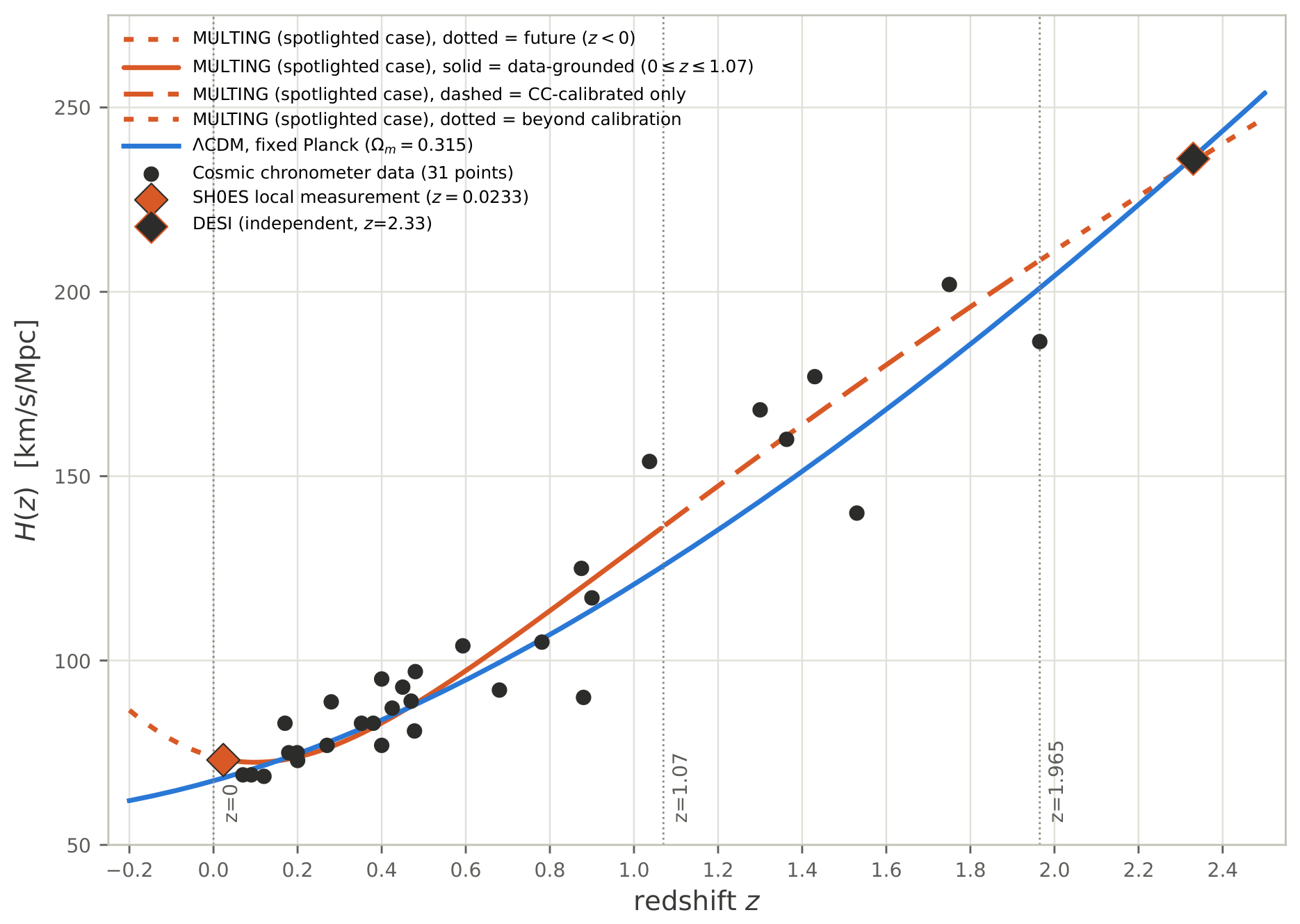
Figure 2.
Data, with visible error bars, and a fair, apples-to-apples CDM comparison. The orange curve is MULTING’s spotlighted case; its SH0ES-anchored comparison case is not separately shown, since the two differ by under across this entire range, visually indistinguishable at this scale. The solid blue curve is flat CDM anchored to Planck, as in Figure 1; the dashed blue curve is flat CDM anchored to SH0ES exactly, the same apples-to-apples benchmark used in Section 3. Error bars on the SH0ES point, the 31 Cosmic Chronometer points, and the DESI point are each the real, reported uncertainty. The SH0ES and DESI error bars are similar in relative terms ( and of their respective central values), but the DESI bar appears substantially larger in the plot, since DESI’s absolute uncertainty ( km/s/Mpc) is nearly three times SH0ES’s ( km/s/Mpc) on this shared, absolute vertical scale.
Figure 2.
Data, with visible error bars, and a fair, apples-to-apples CDM comparison. The orange curve is MULTING’s spotlighted case; its SH0ES-anchored comparison case is not separately shown, since the two differ by under across this entire range, visually indistinguishable at this scale. The solid blue curve is flat CDM anchored to Planck, as in Figure 1; the dashed blue curve is flat CDM anchored to SH0ES exactly, the same apples-to-apples benchmark used in Section 3. Error bars on the SH0ES point, the 31 Cosmic Chronometer points, and the DESI point are each the real, reported uncertainty. The SH0ES and DESI error bars are similar in relative terms ( and of their respective central values), but the DESI bar appears substantially larger in the plot, since DESI’s absolute uncertainty ( km/s/Mpc) is nearly three times SH0ES’s ( km/s/Mpc) on this shared, absolute vertical scale.
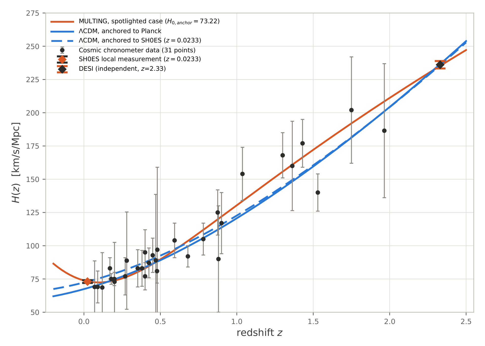

Table 1.
Aspects regarding two known eras in the rate of expansion of the universe and one possibly impending era in the rate of expansion of the universe. The redshift links with the time 7.5 gigayears after the Big Bang. The redshift links with the time 9.0 gigayears after the Big Bang.
Table 1.
Aspects regarding two known eras in the rate of expansion of the universe and one possibly impending era in the rate of expansion of the universe. The redshift links with the time 7.5 gigayears after the Big Bang. The redshift links with the time 9.0 gigayears after the Big Bang.
| Era | Approximate starting time | Approximate ending time |
|---|---|---|
| Decreasing positive rate of expansion | Less than one second after the Big Bang | The start of the next era |
| Increasing positive rate of expansion | Approximately 7.5 to 9 billion years after the Big Bang | The start of the next era, if there will be a next era |
| Possibly decreasing rate of expansion | Perhaps around or after 14 billion years after the Big Bang | - |
Table 2.
Fit qualities, across the range between the SH0ES and Planck anchors, for 33-point fits. SH0ES is treated as a data point at , the lower bound of the real Hubble-flow sample underlying the SH0ES measurement, rather than at (Section 4.12 discusses this choice and its robustness). Each row lists an value (usually, but not always, between the Planck value and the SH0ES value ) and then the optimized values of and . Optimization is against all 33 points (31 Cosmic Chronometer, SH0ES, and DESI). denotes chi-squared for 33 data points. denotes Pearson-r for 33 data points. measures how well the fitted curve matches all 33 points, including SH0ES and DESI, given the value for that row. The next-to-right-most column states the “distance,” in standard deviations of the combined Planck-SH0ES uncertainty (), that sits from SH0ES. For the positive value, is larger than . For the negative values, is smaller than . The right-most column states the “distance”, in standard deviations of the combined Planck-SH0ES uncertainty (), that sits from Planck. For the last six rows, which lie on or between and , the magnitudes of the next-to-right-most and right-most columns always sum to exactly the full Planck-SH0ES tension. The first row, for which overshoots SH0ES rather than sitting between and , breaks the previous pattern; the two magnitudes sum to . For each one of the seven rows, two distances are independent of , not restatements of it. Rows are sorted by distance from Planck, descending.
Table 2.
Fit qualities, across the range between the SH0ES and Planck anchors, for 33-point fits. SH0ES is treated as a data point at , the lower bound of the real Hubble-flow sample underlying the SH0ES measurement, rather than at (Section 4.12 discusses this choice and its robustness). Each row lists an value (usually, but not always, between the Planck value and the SH0ES value ) and then the optimized values of and . Optimization is against all 33 points (31 Cosmic Chronometer, SH0ES, and DESI). denotes chi-squared for 33 data points. denotes Pearson-r for 33 data points. measures how well the fitted curve matches all 33 points, including SH0ES and DESI, given the value for that row. The next-to-right-most column states the “distance,” in standard deviations of the combined Planck-SH0ES uncertainty (), that sits from SH0ES. For the positive value, is larger than . For the negative values, is smaller than . The right-most column states the “distance”, in standard deviations of the combined Planck-SH0ES uncertainty (), that sits from Planck. For the last six rows, which lie on or between and , the magnitudes of the next-to-right-most and right-most columns always sum to exactly the full Planck-SH0ES tension. The first row, for which overshoots SH0ES rather than sitting between and , breaks the previous pattern; the two magnitudes sum to . For each one of the seven rows, two distances are independent of , not restatements of it. Rows are sorted by distance from Planck, descending.
Table 3.
Force-term decomposition, as a share of the gross force budget, . “Net” is the signed sum of the four preceding columns: the small residual that enters the equation of motion, after the near-total cancellation between and . For each of Table 3 and Table 3, subsequent rows link to later times.
Table 3.
Force-term decomposition, as a share of the gross force budget, . “Net” is the signed sum of the four preceding columns: the small residual that enters the equation of motion, after the near-total cancellation between and . For each of Table 3 and Table 3, subsequent rows link to later times.
| Force-term decomposition, as a share of the gross force budget, for the spotlighted MULTING solution. For this solution,. In this table, subsequent rows link to later times. | |||||
|---|---|---|---|---|---|
| z | net | ||||
| Force-term decomposition, as a share of the gross force budget, for the SHOES-anchored MULTING solution. For this solution,. In this table, subsequent rows link to later times. | |||||
| z | net | ||||
Table 4.
Similarities and differences, regarding types of theory, between MULTING and CDM. The left-most column lists aspects that each one of MULTING and CDM has. The right-most two columns characterize differences with respect to the aspects. Node denotes a node in the cosmic web. A relevant node contains one galaxy cluster or a few galaxy clusters.
Table 4.
Similarities and differences, regarding types of theory, between MULTING and CDM. The left-most column lists aspects that each one of MULTING and CDM has. The right-most two columns characterize differences with respect to the aspects. Node denotes a node in the cosmic web. A relevant node contains one galaxy cluster or a few galaxy clusters.
| Aspect | MULTING | CDM |
|---|---|---|
| Foundational framework | Newtonian | General relativistic |
| Structural approach | Local | Global |
| Structural approach | Bottom-up | Top-down |
| Structural approach | Discrete (or inhomogeneous) | Continuous (or homogeneous) |
| Causal origin | Matter-sourced | Geometry-sourced |
| Causal origin | Multipole expansion | Perfect fluid |
| Empirical scope | Node-scale testable | Horizon-scale testable |
| Empirical scope | Dark-energy-free | Dark-energy-dependent |
Table 5.
Robustness of the spotlighted case to the choice of SH0ES redshift. Each row refits the unconstrained (spotlighted) configuration with SH0ES placed at the stated redshift, across its real range. This demonstrates robustness across the range; it is not an argument that any one row is the most appropriate point.
Table 5.
Robustness of the spotlighted case to the choice of SH0ES redshift. Each row refits the unconstrained (spotlighted) configuration with SH0ES placed at the stated redshift, across its real range. This demonstrates robustness across the range; it is not an argument that any one row is the most appropriate point.
Table 6.
The spotlighted case, across five descriptions, time-ordered. Time since the Big Bang uses the standard 13.8 Gyr (gigayears) age as a fixed reference point for this framework’s own, independently-derived relative timing; it is not itself independently derived here. “LCDM” gives the sign of for flat CDM (fixed Planck) at the same redshift, for comparison, not this framework’s own prediction.
Table 6.
The spotlighted case, across five descriptions, time-ordered. Time since the Big Bang uses the standard 13.8 Gyr (gigayears) age as a fixed reference point for this framework’s own, independently-derived relative timing; it is not itself independently derived here. “LCDM” gives the sign of for flat CDM (fixed Planck) at the same redshift, for comparison, not this framework’s own prediction.
| Time (Gyr since Big Bang) | z | LCDM | net | |||
|---|---|---|---|---|---|---|
| − | - | − | + | |||
| − | - | − | + | |||
| − | + | − | + | |||
| − | + | 0 | + | |||
| 0 | + | + | 0 | |||
| + | + | + | − | |||
| + | + | + | − | |||
| + | + | + | − |
Disclaimer/Publisher’s Note: The statements, opinions and data contained in all publications are solely those of the individual author(s) and contributor(s) and not of MDPI and/or the editor(s). MDPI and/or the editor(s) disclaim responsibility for any injury to people or property resulting from any ideas, methods, instructions or products referred to in the content. |
© 2026 by the authors. Licensee MDPI, Basel, Switzerland. This article is an open access article distributed under the terms and conditions of the Creative Commons Attribution (CC BY) license (http://creativecommons.org/licenses/by/4.0/).
Copyright: This open access article is published under a Creative Commons CC BY 4.0 license, which permit the free download, distribution, and reuse, provided that the author and preprint are cited in any reuse.