

Submitted:
12 August 2026
Posted:
13 August 2026
You are already at the latest version
Abstract
The electrotonic response of a nerve to a subthreshold current pulse has been described as a passive electrical spread in the axolemma since the mid-nineteenth century, and the mathematical formalism of the linear cable equation has been treated as its mechanism ever since Kelvin (1855) and Rall (1957 onwards). We revisit the demonstration that William Rutherford gave to his students at Edinburgh in 1876, restate what he could see and what he could not, and perform three modern in silico experiments in the same demonstrative spirit. The three experiments compare, on the same measured trace, a strict Hodgkin--Huxley formulation, a formulation with independent stimulus and action-potential sources, and a Hodgkin--Huxley formulation augmented ad hoc with variable capacitance and ion-dependent resistance. Only the independent-sources formulation reproduces three routine facts of electrophysiology (all-or-none amplitude, waveform invariance, and coherence of algorithmic artefact subtraction) without a single fitted parameter. We conclude that the electrotonic response is not a passive electrical spread in the axolemma but the vertical projection of a horizontal ionic movement in the periaxonal polyelectrolyte gel adjacent to the axolemma, and that the classical cable equation preserves its descriptive validity as the shadow of that movement while losing its ontological reading as the mechanism.
Keywords:
electrotonus
; nerve conduction
; cable theory
; Hodgkin--Huxley
; periaxonal gel
; ionic-mechano-hydraulic model
“Gentlemen, You have already witnessed the fact that when a continuous galvanic current of equable strength is passed along a motor nerve, contraction of the muscles supplied by the nerve takes place only when the current begins or when it ends, and thatduringthe passage of the current the muscles remain at rest. From this fact you might suppose that the nerve is unaffected during the transmission of the current, but it is not so; the current all the while it traverses the nerve induces in it a peculiar state, termed the electrotonic state or simply electrotonus.”– William Rutherford, On Electrotonus. A Physiological Demonstration, J. Anat. Physiol. 2, 87–103 (1876).
1. Gentlemen
One hundred and fifty years ago in the Physiological Laboratory of the University of Edinburgh, William Rutherford stood in front of a room of gentlemen and, using a Pohl commutator, a Du Bois Reymond key, a Grove’s battery, and the sciatic nerve of a freshly prepared frog, demonstrated in a single session the three laws of electrotonus: the variation of nervous excitability under the two poles of a continuous galvanic current, the variation of the rate of nervous conduction, and the variation of the electromotive power of the nerve itself.
The demonstration was rigorous. The observations were reproducible. The vocabulary that Rutherford introduced to name what he had shown, Anelectrotonus for the state induced by the positive pole, Cathelectrotonus for that induced by the negative pole, the neutral point of Pflüger, the extrapolar and intrapolar portions of the nerve, has entered the physiological lexicon and is with us today.
Yet, at the very end of his demonstration, Rutherford stopped and admitted the following, verbatim:
A crowd of theoretical considerations surrounds this most interesting subject. Are the changes which constitute electrotonus due to electrolysis of the nerve? Does the − pole increase the development of nerve force from chemical force, while it hinders its conversion into electrical force, and vice versa with the + pole? Is increased excitability of a nerve due to a higher tension of the nerve force, whereby its discharge is rendered more easy? […] But we have already exhausted our time, and must postpone these considerations until our next demonstration.
It should be noted that Rutherford, an illustrious researcher acting in the best faith of his time, closed his demonstration on an open question rather than on a verdict. He described what he could see with the instruments of 1876 and he left to a next demonstration what he could not yet answer. This paper is that next demonstration. It has been considerably delayed.
2. What Rutherford Could Not Know
The nerve force that Rutherford invoked was a placeholder for physics that had not yet been formulated. The molecular biology of the axon, the voltage-dependent ion channel, the patch-clamp technique, the periaxonal polyelectrolyte gel, and the imaging methods that today let us look at the axolemma at nanometric resolution were all still to come. It is not surprising that the framework which eventually filled the placeholder followed the mathematics rather than the physics.
The mathematical filler was the linear cable equation. Kelvin (1855) had derived it for the trans-Atlantic telegraphic cable [2]. Rall (1957 onwards) adapted it to the biological cable and made it the substrate of what would become the compartmental simulator of computational neuroscience (NEURON, GENESIS, and every architecture inheriting from them). The cable equation, applied to a passive membrane, describes the electrotonic response of the axolemma with a length constant and a time constant that match measurement well within experimental precision.
Hodgkin and Huxley (1952) then took the same passive-cable equation and added to it a set of voltage-dependent conductances at each patch of membrane [6]. The action potential became, in this framework, a regenerated electrotonus: the same cable equation with a self-reinforcing term. The passive electrotonic response was the substrate; the action potential was its regenerative amplification.
The move was elegant, mathematically consistent, and empirically successful for the observables it was fitted against. It also fused two very different physical events into a single conceptual object. The subthreshold electrotonus, taken as a passive electrical spread in the axolemma, became the mother of the suprathreshold action potential, taken as its regenerated form. The bridge held for seventy years.
3. The Cracks in the Story
The story cracked long ago, in the literature that is supposed to support it.
Rosenberg (1937) [3], whose paper on the physico-chemical basis of electrotonus is itself one of the historical pillars of the cable-equation reading, documented in the very same paper that the theoretical prediction of his three-parameter chain-conductor model was quantitatively wrong. On page 1032 he wrote: “the theoretical curve is initially steeper and subsequently flatter than the experimental curve”. On page 1033 he added: “the capacity gradually increases”. The founder of the mathematical formalism admitted, in the same paper that introduced the formalism, that the formalism failed to match the shape of the measured curves and that the capacitance was not a fixed material parameter but something that varied during the response.
Bouman (1937) [4], in the same year, was even more direct. In a series of experimental tables (Tables VI to XIII of his paper), he showed that the electrotonic response depended strongly on the ionic composition of the bath. Excess abolished the catelectrotonic effect entirely. Excess inverted it. Prolonged also inverted it. In the language of the framework that would come to dominate physiology fifteen years later, Bouman had shown that the electrotonus is ionic in its response, not merely electrical. Hill (1936) [5], in a related paper, wrote in this connection that “electrotonus is a separate phenomenon from excitation”.
Hellerstein (1968) [7], thirty years later, produced the mathematical generalisation. His Figure 1 explicitly distinguishes applied sources (, ) from induced currents (, ). The formalism of independent superposition existed, in publication, from that date onwards. It has been available in the cable-equation literature for nearly sixty years. It has almost never been read as a diagnostic of the framework.
The cracks were in the literature all along; the community read them as details, not as diagnosis.
4. The Question Rutherford Did Not Ask, but Which We Must Ask Today
Given the cracks, the question follows on its own. Rutherford could not ask it in 1876 because the vocabulary was not yet available. We can ask it now.
Is the electrotonus really electrical?
Or is the measured potential at the axolemma the vertical projection of a horizontal ionic movement in a compartment adjacent to the axolemma, a compartment whose existence and material properties were unknown to Rutherford and were only slowly documented across the twentieth and early twenty-first centuries?
If the electrotonus is truly a passive electrical spread in the axolemma, why does replacing the extracellular with abolish it? Why does excess invert it? Why does prolonged invert it as well?
And if we take Occam’s razor to the two readings, which one requires fewer ad hoc parameters?
The next section performs the demonstration in three configurations, in the spirit of Rutherford at the myograph, but with the instruments of 2026.
5. A Demonstration in Three Configurations
Gentlemen, we now propose to perform three in silico experiments. Each shows what happens on the measured voltage trace when a subthreshold-to-suprathreshold current pulse is applied and an action potential is triggered, under three distinct physical assumptions about the underlying substrate. The three circuits and the three families of traces are shown in Figure 1, Figure 2, Figure 3 and Figure 4.
5.1. Configuration A: Strict Hodgkin–Huxley
Under strict Hodgkin–Huxley, the stimulus current is a transmembrane current injected into the same patch of axolemma where the voltage-gated Na and K channels are located. The three currents (stimulus, Na, K) close their loops in the same extracellular volume, assumed to be a homogeneous conductor. Kirchhoff’s laws apply to the combined circuit. The prediction is unambiguous: during any period of temporal overlap between the stimulus and the rising phase of the action potential, the two contributions add linearly on the measured trace, and the observed amplitude depends on the amplitude of the stimulus.
Figure 2 shows the measured trace for three amplitudes of the stimulus pulse: , , and threshold. You see the shape of the rising phase depend on the amplitude of the stimulus; the peak amplitude is shifted by the residual stimulus current; and the latency between stimulus onset and action-potential peak shortens as the stimulus amplitude increases. Every trace carries the fingerprint of the stimulus.
5.2. Configuration B: Independent Sources
Under the independent-sources configuration, the stimulus and the action potential are in two physically distinct substrates. The stimulus displaces ions in the extracellular volume accessible from the recording electrode, producing a broadband electrical signature (the artefact of the artefact-removal literature, of which Wang et al. [9] is one representative recent example). The action potential, once triggered, is a stereotyped biphasic event whose amplitude and waveform are determined by the intrinsic properties of the source, not by the stimulus that triggered it. The two signatures superpose on the recording amplifier only at the level of the measurement.
Figure 3 shows the same three amplitudes. You see the amplitude and shape of the action potential invariant across the three cases; only the stimulus artefact varies with the stimulus amplitude. This is the all-or-none amplitude that every student learns in the first weeks of neurophysiology. It is the biology.
5.3. Configuration C: Hodgkin–Huxley Augmented Ad Hoc
The defender of Hodgkin–Huxley may now object that the framework can be augmented. We allow it. Configuration C is Configuration A supplemented with a voltage-dependent capacitance (in the spirit of Rosenberg’s own observation that “the capacity gradually increases”) and an ion-dependent transverse resistance (in the spirit of Bouman’s tables). With enough parameters, Configuration C can be tuned to approach the behaviour of Configuration B on any given experimental preparation.
Figure 4 shows the result of one such tuning. The and traces are drawn closer to the amplitude-invariance target than in Configuration A, but the effective threshold has shifted upwards: the trace no longer fires. A different preparation, a different bath composition, a different stimulus waveform would require a different parameter set. This is not physical modelling. It is curve fitting.
5.4. Summary
Table 1 confronts the three configurations to the three routine facts of the discipline.
6. Verdict
Under strict Hodgkin–Huxley, the true summation predicted by Kirchhoff’s laws is not observed.
Under the augmented ad hoc version, each new experimental fact costs a new adjustable parameter: this is no longer physical modelling, it is curve fitting.
Only the independent-sources configuration reproduces the observed biology without a single fitted parameter.
7. What Rutherford Was Searching for
We return, in closing, to Rutherford at the myograph. The nerve force he invoked at the end of his demonstration was a placeholder for the physics that was not yet available. Today, one hundred and fifty years later, we can say what filled it.
The electrical variable that Rutherford was measuring at the axolemma was not itself the mechanism. It was the vertical projection, onto the electrical dimension of measurement, of a horizontal ionic movement in a compartment that Rutherford could not see: the periaxonal polyelectrolyte gel adjacent to the axolemma, a nanometric structured hydrated matrix bounded by the axolemma inside, the myelin or Schwann-cell membrane outside, and the paranodal tight junctions of claudin-1, claudin-2, ZO-1, and occludin at each end of an internode.
The cable equation of Kelvin and Rall preserves its descriptive validity. It describes the vertical shadow accurately. What it does not describe is the horizontal mechanism.
The ionic-mechano-hydraulic (IMH) framework, developed in Delalande and Tamagawa (2026) [8], places the mechanism where the physics is: in the ionic movement and the coupled mechanical response of the periaxonal gel. Under IMH, the electrotonus is the shadow of a subthreshold ionic redistribution; the action potential is the shadow of a suprathreshold ionic-mechanical wave; the transition between the two regimes is the threshold of a mechanical actuator, not the threshold of an electrical regeneration.
Rutherford closed his demonstration on a question. We close ours on the same question, answered as far as the physics available today allows.
The authors used large language model (LLM) assistants (Claude, Anthropic) during the preparation of this manuscript for tasks that included literature search, editing, and paragraph writing. All scientific content, theoretical claims, and conclusions are the sole responsibility of the authors. The authors have reviewed and verified all AI-assisted content.
Author Contributions
Conceptualization, B.D. and H.T.; methodology, B.D.; software, B.D.; formal analysis, B.D. and H.T.; investigation, B.D.; writing—original draft preparation, B.D.; writing—review and editing, B.D. and H.T. All authors have read and agreed to the published version of the manuscript.
Funding
This research received no external funding.
Data Availability Statement
The three SPICE netlists (ngspice), the Python simulation scripts, and the matplotlib post-processing scripts used to produce Figure 2, 3, and 4 are available on request and will be deposited on Zenodo alongside the accepted version of this preprint.
Conflicts of Interest
The authors declare no conflict of interest.
References
- Rutherford, W. On Electrotonus. A Physiological Demonstration given in the Physiological Laboratory of the University of Edinburgh. J. Anat. Physiol. 1876, 2, 87–103. [Google Scholar]
- Thomson, W. On the theory of the electric telegraph. Proc. R. Soc. Lond. 1855, 7, 382–399. [Google Scholar] [CrossRef]
- Rosenberg, H. The physico-chemical basis of electrotonus. Trans. Faraday Soc. 1937, 33, 1028–1035. [Google Scholar] [CrossRef]
- Bouman, H.D. The effect of electrotonus on the excitability of nerve. J. Physiol. 1937, 89, 32–44. [Google Scholar] [CrossRef] [PubMed]
- Hill, A.V. Excitation and accommodation in nerve. Proc. R. Soc. B 1936, 119, 305–355. [Google Scholar] [CrossRef]
- Hodgkin, A.L.; Huxley, A.F. A quantitative description of membrane current and its application to conduction and excitation in nerve. J. Physiol. 1952, 117, 500–544. [Google Scholar] [CrossRef] [PubMed]
- Hellerstein, D. Passive membrane potentials: a generalization of the theory of electrotonus. Biophys. J. 1968, 8, 358–379. [Google Scholar] [PubMed]
- Delalande, B.; Tamagawa, H. How does the nerve impulse travel? Mechanical, structural and thermal dimensions of nerve conduction. Prog. Biophys. Mol. Biol. 2026, 201, 299–310. [Google Scholar] [CrossRef] [PubMed]
- Wang, F.; Chen, X.; Roelfsema, P.R. Comparison of electrical microstimulation artifact removal methods for high-channel-count prostheses. J. Neurosci. Methods 2024, 408, 110169. [Google Scholar] [CrossRef] [PubMed]
Figure 1.
Circuit diagrams of the three configurations. Configuration A (strict Hodgkin–Huxley) is a patch of axolemma with membrane capacitance in parallel with three ionic branches (voltage-dependent Na, voltage-dependent K, and passive leak); the stimulus current source closes its loop in the same extracellular volume as the endogenous currents (shared substrate, Kirchhoff summation obligatory). Configuration B (independent sources) has two strictly decoupled loops: a stimulus generator with its own extracellular return , and a stereotyped-AP voltage source with a confined periaxonal-gel return ; the recorded trace is the arithmetic sum at the amplifier, with no physical interaction between the two substrates. Configuration C (Hodgkin–Huxley augmented ad hoc) is Configuration A with two fitting handles added: a voltage-dependent membrane capacitance (in the spirit of Rosenberg’s “the capacity gradually increases”), and an ion-dependent transverse resistance (in the spirit of Bouman’s ionic-composition tables); the Na conductance carries a stimulus-amplitude-dependent damping factor .
Figure 1.
Circuit diagrams of the three configurations. Configuration A (strict Hodgkin–Huxley) is a patch of axolemma with membrane capacitance in parallel with three ionic branches (voltage-dependent Na, voltage-dependent K, and passive leak); the stimulus current source closes its loop in the same extracellular volume as the endogenous currents (shared substrate, Kirchhoff summation obligatory). Configuration B (independent sources) has two strictly decoupled loops: a stimulus generator with its own extracellular return , and a stereotyped-AP voltage source with a confined periaxonal-gel return ; the recorded trace is the arithmetic sum at the amplifier, with no physical interaction between the two substrates. Configuration C (Hodgkin–Huxley augmented ad hoc) is Configuration A with two fitting handles added: a voltage-dependent membrane capacitance (in the spirit of Rosenberg’s “the capacity gradually increases”), and an ion-dependent transverse resistance (in the spirit of Bouman’s ionic-composition tables); the Na conductance carries a stimulus-amplitude-dependent damping factor .
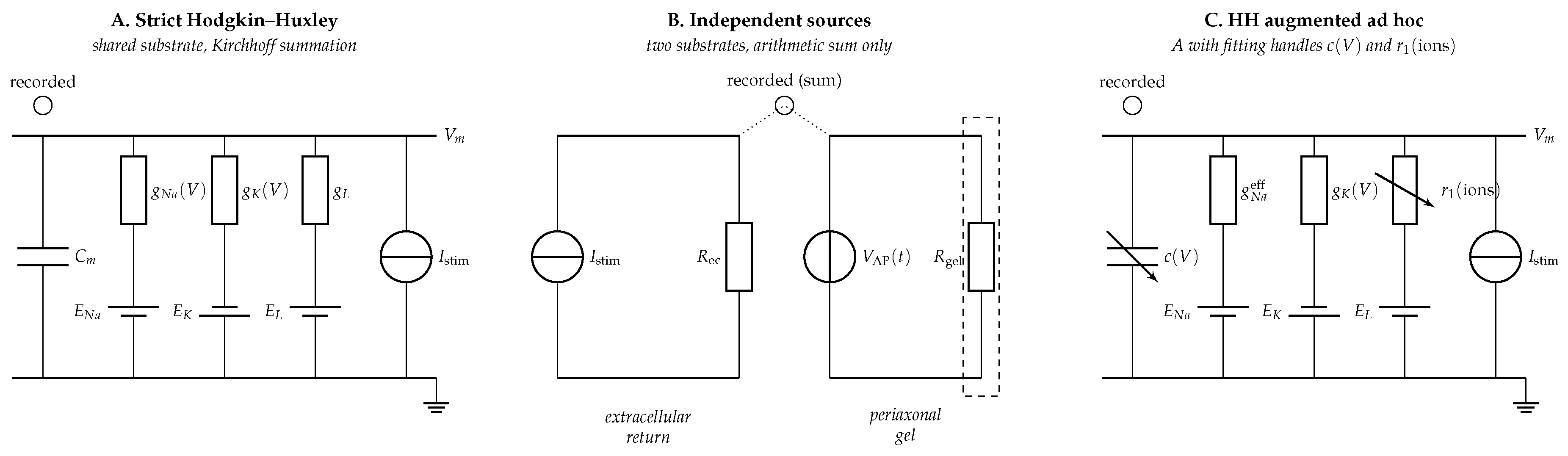
Figure 2.
Configuration A (strict Hodgkin–Huxley). Voltage response at the stimulated patch for three stimulus amplitudes (, , threshold). The stimulus fingerprint is visible on every trace; the shape of the rising phase and the peak amplitude are stimulus-dependent.
Figure 2.
Configuration A (strict Hodgkin–Huxley). Voltage response at the stimulated patch for three stimulus amplitudes (, , threshold). The stimulus fingerprint is visible on every trace; the shape of the rising phase and the peak amplitude are stimulus-dependent.
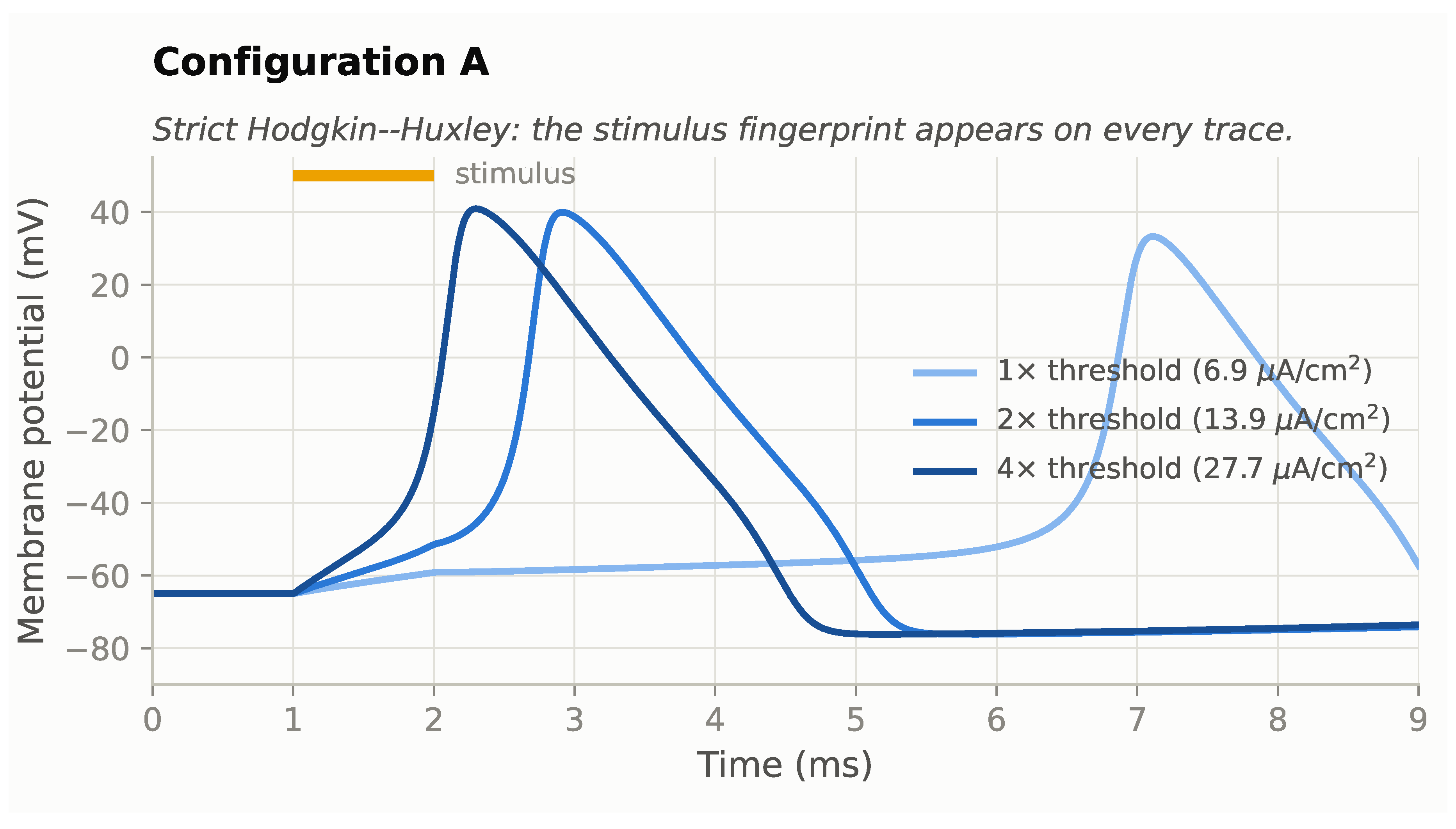
Figure 3.
Configuration B (independent sources). Voltage response for three stimulus amplitudes (, , threshold). The action potential template used here is the Hodgkin–Huxley waveform itself, extracted from the Configuration A substrate at threshold and replayed as an independent source. The action potential is invariant in amplitude and shape; only the stimulus artefact varies with the stimulus amplitude.
Figure 3.
Configuration B (independent sources). Voltage response for three stimulus amplitudes (, , threshold). The action potential template used here is the Hodgkin–Huxley waveform itself, extracted from the Configuration A substrate at threshold and replayed as an independent source. The action potential is invariant in amplitude and shape; only the stimulus artefact varies with the stimulus amplitude.
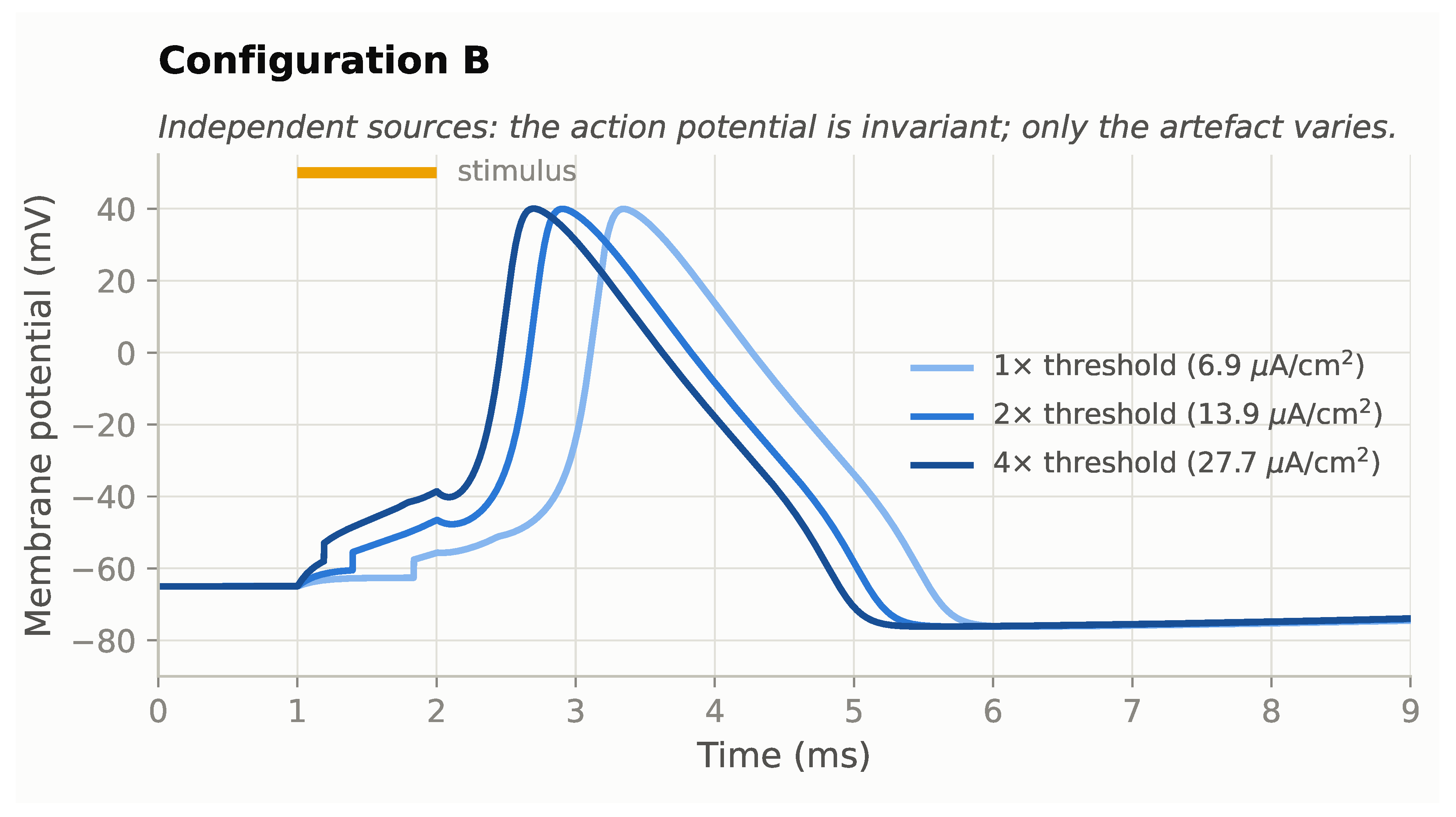
Figure 4.
Configuration C (Hodgkin–Huxley augmented ad hoc). Voltage response for three stimulus amplitudes (, , threshold). The traces approach those of Configuration B on the and amplitudes, but only for a particular tuning of and ; the effective threshold shifts and the amplitude no longer fires.
Figure 4.
Configuration C (Hodgkin–Huxley augmented ad hoc). Voltage response for three stimulus amplitudes (, , threshold). The traces approach those of Configuration B on the and amplitudes, but only for a particular tuning of and ; the effective threshold shifts and the amplitude no longer fires.
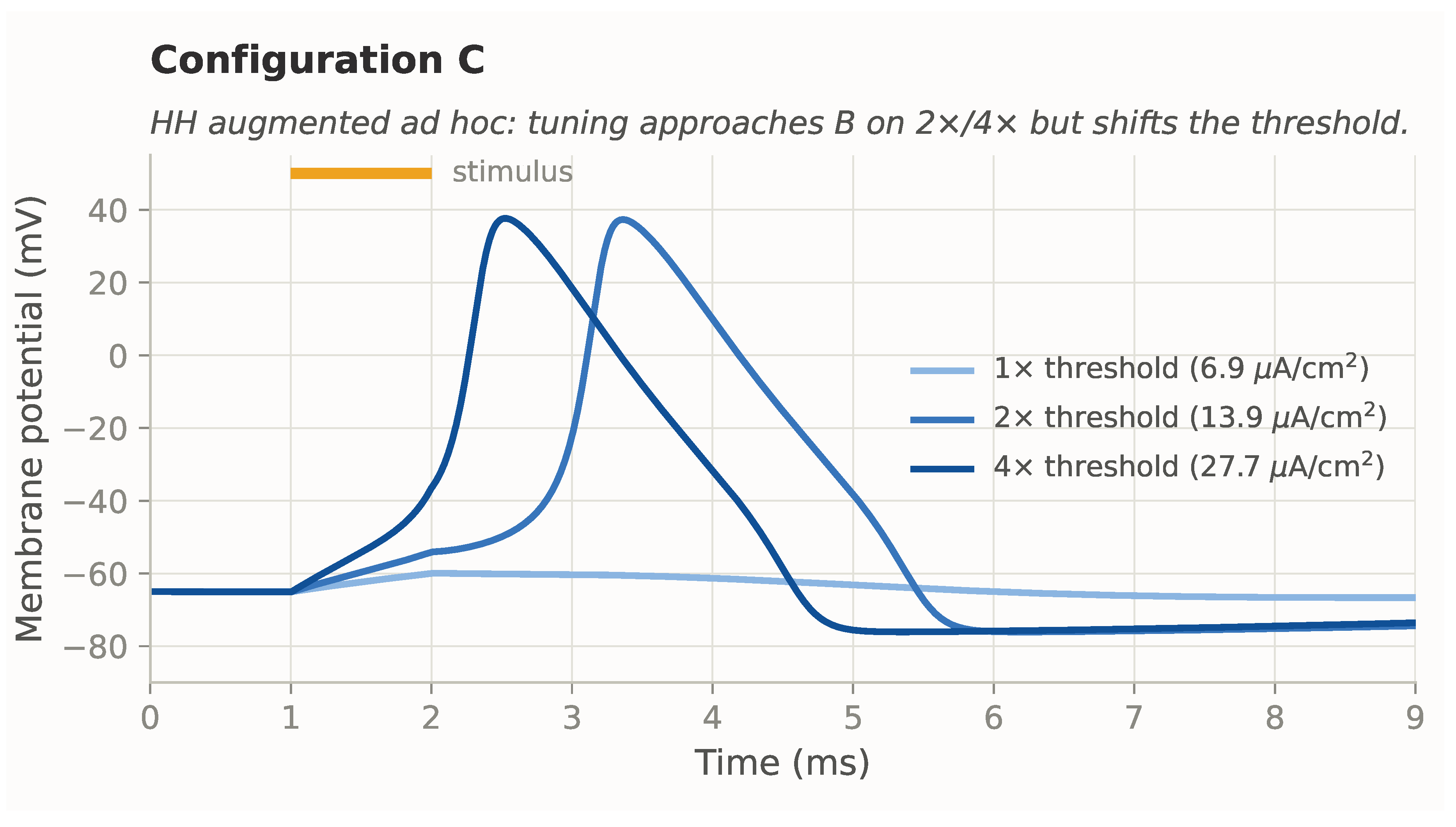

Table 1.
Predictions of the three configurations for three routine facts of electrophysiology. Configuration A fails systematically. Configuration B succeeds natively. Configuration C succeeds only at the cost of parameter tuning per preparation.
Table 1.
Predictions of the three configurations for three routine facts of electrophysiology. Configuration A fails systematically. Configuration B succeeds natively. Configuration C succeeds only at the cost of parameter tuning per preparation.
| Observable fact | Config. A | Config. B | Config. C |
|---|---|---|---|
| All-or-none amplitude of the AP under supra-threshold stimuli | Fails: shifts with stimulus | Native invariance | Achievable by tuning |
| Waveform of the AP independent of the stimulus waveform | Fails: tinted during overlap | Native invariance | Achievable by tuning |
| Post-hoc artefact subtraction recovers the AP intact | Fails: interaction residues | Native: no interaction | Achievable by tuning |
Disclaimer/Publisher’s Note: The statements, opinions and data contained in all publications are solely those of the individual author(s) and contributor(s) and not of MDPI and/or the editor(s). MDPI and/or the editor(s) disclaim responsibility for any injury to people or property resulting from any ideas, methods, instructions or products referred to in the content. |
© 2026 by the authors. Licensee MDPI, Basel, Switzerland. This article is an open access article distributed under the terms and conditions of the Creative Commons Attribution (CC BY) license.
Copyright: This open access article is published under a Creative Commons CC BY 4.0 license, which permit the free download, distribution, and reuse, provided that the author and preprint are cited in any reuse.