

Submitted:
07 August 2026
Posted:
11 August 2026
You are already at the latest version
Abstract
The decarbonisation of the energy sector requires efficient strategies to reduce fuel consumption and greenhouse gas emissions. Organic Rankine Cycles (ORCs) have emerged as a promising technology for waste heat recovery due to their flexibility and ability to operate with low- and medium-temperature heat sources. This work develops a general mathematical framework, grounded in the Helmholtz energy function, to characterise the limiting and optimal efficiency of ORCs equipped with an Internal Heat Exchanger (IHE) when operating with dry and isentropic working fluids. The framework is exemplified using the van der Waals equation of state and extended to real fluids through the PC-SAFT model. Results show that integrating an IHE significantly enhances efficiency for drier working fluids, which expand deeper into the superheated vapour region, enabling greater internal heat recovery. Efficiency gains diminish at condenser temperature extremes, defining operational boundaries where IHE integration is less effective. From a practical perspective, minimising the temperature difference at the IHE outlet (ΔTmin) is critical to maximise performance. The proposed framework provides theoretical insight and practical guidelines for fluid selection and operating strategies in ORC-based waste heat recovery systems.
Keywords:
Organic Rankine Cycle
; internal heat exchanger
; operational conditions
; optimal conditions
; efficiency
1. Introduction
The decarbonisation of the energy sector is one of the major technological and scientific challenges of the twenty-first century. Although renewable energy technologies have expanded rapidly, fossil fuels continue to dominate the global primary energy supply and remain the largest source of anthropogenic greenhouse gas emissions [1,2]. Consequently, improving the efficiency of existing energy conversion systems has become an immediate and cost-effective strategy for reducing fuel consumption and emissions while maximising the utilisation of available energy resources, complementing the long-term transition towards low-carbon energy systems [3,4]. It is estimated that nearly 72 % of the global primary energy supply is lost during energy conversion and ultimately dissipated into the environment as low- or medium-temperature waste heat [5]. Therefore, as a strategy to improve energy efficiency, waste heat recovery (WHR) has attracted significant research interest in industrial processes [6]. Converting this underutilised energy into useful power offers an effective pathway to improve overall system efficiency while reducing fuel consumption and emissions [6,7]. Several technologies have been proposed for this purpose, including the conventional Rankine cycle, the Kalina cycle, supercritical carbon dioxide (sCO2) cycles, high-temperature heat pumps, and Organic Rankine Cycles (ORCs) [3,8]. Among the available WHR technologies, the ORC has emerged as one of the most promising solutions owing to its simple configuration, operational flexibility, and ability to efficiently recover low- and medium-temperature heat using organic working fluids with favourable thermophysical properties [7,8,9]. In recent years, various strategies have been studied to improve the thermodynamic performance of the ORC, including the development and selection of novel working fluids [10], the use of zeotropic mixtures [11], transcritical [12] and supercritical [13] configurations, multi-pressure cycles [14], multiple heat-source configurations [15], reheating processes [16], cascade configurations [17], and thermo-economic optimisation methodologies [18]. Among these alternatives, incorporating an Internal Heat Exchanger (IHE), also referred to as an internal recuperator, can significantly enhance the thermodynamic performance of ORCs by recovering part of the thermal energy contained in the turbine exhaust to preheat the working fluid before evaporation [18]. This internal heat recovery reduces the external heat input required, leading to higher thermal efficiencies, particularly when dry or isentropic working fluids are employed [7,19]. Accordingly, considerable research has focused on evaluating the influence of the IHE under different operating conditions, cycle configurations, heat sources, and working fluids. For example, Nondy et al. [20] reported that incorporating an IHE increased the thermal efficiency from 12.76 % to 14.07 % and the exergy efficiency from 43.31 % to 47.46 %, although the net power output decreased from 768.43 to 710.21 kW. Similarly, Braimakis et al. [21] found that the maximum thermal efficiency increased from 18.02 % for a conventional ORC to 22.85 % after incorporating an IHE. Safarian et al. [22] observed that thermal efficiency increased from 19.46 % to 21.50 %, accompanied by an increase in net power output from 49.04 to 54.30 kW. Likewise, Mohammadzadeh Bina et al. [23] showed that the IHE enhanced system performance under all optimisation criteria; under maximum thermal efficiency conditions, thermal efficiency increased from 17.69 % to 20.57 %, exergy efficiency from 55.14 % to 63.72 %, and net power output from 1504 to 2481 kW. Mosaffa et al. [24] also reported improvements in thermal and exergy efficiencies, from 33.21 % to 35.76 % and from 34.99 % to 38.58 %, respectively, for ORCs integrated with liquefied natural gas cold energy. More recently, analytical thermodynamic formulations have emerged as an alternative to conventional numerical optimisation for identifying the limiting conditions associated with the maximum performance of ORCs. Ahmed et al. [25] theoretically demonstrated that the thermal efficiency of conventional ORCs may exhibit a maximum in the subcritical region, showing that increasing the maximum cycle temperature does not necessarily lead to higher thermal efficiency and that this behaviour depends on the thermodynamic properties of the working fluid. Moreover, subsequent studies developed analytical formulations based on the Helmholtz free energy to determine the operating conditions associated with maximum cycle performance [26,27]. This framework was later extended to hybrid systems combining vapour-compression refrigeration and an ORC, enabling the analytical identification of maximum thermal efficiency, maximum net power output, and the optimum operating range of the integrated system [28].
This work presents a framework to determine the optimal conditions for achieving maximum efficiency of a dry working fluid used in an ORC with an IHE. The proposed framework is based on a general Helmholtz energy function with direct application to any model, and its rudiments are exemplified with the van der Waals equation of state (EOS). Moreover, applications to real working fluids are developed with the PC-SAFT EOS. The working fluids are selected to enable a thorough analysis and to provide guidelines for establishing optimal operating conditions to achieve higher ORC efficiency.
2. Thermodynamic Theory and Modelling
The ORC with an IHE is displayed in Figure 1a and consists of a condenser, a pump, a boiler, a turbine, and an IHE. The IHE recovers part of the thermal energy at the turbine outlet; the recovered energy is delivered to the pump outlet to preheat the working fluid before it enters the boiler. Figure 1b shows the temperature profile in the IHE, which uses a parallel flow for straightforward representation. However, the IHE can operate in either counter-flow or parallel-flow configuration. There are two flows in the IHE: a high-temperature and a low-temperature one. The high-temperature flow is the working fluid from the turbine outlet (red line). The low-temperature flow is the working fluid from the pump outlet (blue line). In Figure 1b, the temperature difference between the flows at the IHE outlet must always be positive. Therefore, the temperature of the high-temperature flow at the IHE outlet, , is always higher than that of the low-temperature flow, , i.e., .
Figure 2 shows the projection of temperature vs entropy for a basic ORC and an ORC with an IHE. Figure 2a shows the basic ORC that expands from a maximum entropy point [29]. Figure 2b shows the ORC with an IHE that expands from a point with a higher temperature than the maximum entropy point. Those points have been shown to provide both higher thermal efficiency and net power output [26,27,30]. Both ORC configurations share the same base process. The process begins with a pump (1) that compresses a saturated liquid through a quasi-adiabatic isentropic process from low to high pressure (2). The boiler performs an isobaric process from the pump outlet to (3) by adding heat, and from (3) to (4), a quasi-isentropic expansion delivers mechanical work. Finally, the working fluid passes through the condenser, rejecting heat to reach the saturated liquid condition (1) and complete the cycle. For an ORC with an IHE, the working fluid from the turbine outlet passes through the IHE, delivering the energy of its superheated vapour, , up to condition (a). This is delivered to the low-temperature working fluid from the pump outlet up to condition (b). For real working fluids (like n-butane), the minimum temperature difference is 5 °C, as shown in Figure 2b.
The thermal efficiency of a power cycle is the measure of the percentage of the thermal energy supplied to a system that is converted into useful mechanical or electrical work. The thermal efficiency of an ORC is given by the ratio between net power output, , and the heat added in the ORC system, . It is considered that can be written as , where is the amount of heat extracted in the condenser. The above yields
is defined as the heat added in the boiler, , minus the recovered heat in the IHE, , hence, . Moreover, is also defined as the heat delivered in the condenser, , minus the heat delivered by the IHE, , hence, . Therefore, the thermal efficiency for an ORC with an IHE yields
where each heat term is based on enthalpy, , and on turbine and pump performance terms, and , respectively. The subscript i represents the control points presented in Figure 1 and Figure 2. Considering the effects of and , the control points at the outlet of the compression and expansion take the following expressions: the irreversible pump outlet is equal to , and the irreversible turbine outlet is equal to . Therefore, the heat terms can be written as
In the same way that Gonzalez’s works [26,27] show that the maximum efficiency and maximum net power output exist for a basic ORC that expands from a saturated condition, maximum efficiency and maximum net power output also exist for an ORC with an IHE. Both maxima can be found by the efficiency derivative and the net power output derivative for a basic ORC and an ORC with an IHE. On the one hand, mathematical expressions for determining the maximum efficiency and net power output of a basic ORC were developed in the same works [26,27]. On the other hand, this work develops the mathematical expression for determining the maximum efficiency for an ORC with an IHE, whereas the expression for the maximum net power output is the same as in the previous work. The mathematical expression for determining the maximum efficiency can be written as a function of enthalpy as
it can be seen that the mathematical expression for determining the maximum efficiency of an ORC with an IHE does not depend on machinery performance (, ). Considering that is equal to zero [26], the expanded expression becomes
therefore, describing Eq. (7) completely is reduced to describing the derivatives of stages (3), (a), and (b). Following the above, a general structure for the derivatives can be written as [28]
where is the pressure at point i. Moreover, the partial derivatives can be obtained directly by differentiating the Gibbs energy function. Furthermore, the partial derivatives of the thermodynamic functions can be obtained using systematic Legendre transforms and Rowlinson’s shortcut [31]. Details on the partial derivatives of the Gibbs and Helmholtz energy functions can be found in Gonzalez’s work [26]. In the literature, some derivatives of the states (a) and (b) are not described. Both and are written in terms of the Gibbs energy function and its respective Legendre transforms as
Additionally, is equal to zero, since the variation of as a function of is null, because is equal to and , and both pressures are constant.
2.1. Modelling
To predict the properties of working fluids, two EOS have been used. On the one hand, the van der Waals EOS [32,33] is a useful and simple qualitative tool to study complex behaviour topologically [34]. The aforementioned EOS is given by
where is the residual Helmholtz energy function, is the molar volume, R is the universal gas constant, T is the thermodynamic temperature, and a and b are the dispersive constant and the covolume, respectively. On the other hand, the EOS of the SAFT family [35,36] are molecular models based on statistical mechanics principles [37,38] capable of rendering the phase behaviour and thermophysical properties of a wide variety of compounds [39]. One of the most widely used SAFT variants is the PC-SAFT EOS [40,41,42], which is highly recognised for its versatility and accuracy. In the PC-SAFT structure, the contributions to the Helmholtz energy function encompass different physical characteristics of the molecule, such as hard-chain and dispersive contributions. The structure yields
The superscripts in Eq. (12) concern hard-chain and dispersive contributions, respectively [40]. The molecular parameters for the PC-SAFT EOS of the analysed working fluids are detailed in Table 1. The total Helmholtz energy function is the sum of the residual contribution and the ideal contribution, i.e., , where the ideal contribution is given by
In Eq. (13), R is the universal gas constant and and are the thermodynamic temperature and pressure of a reference state, , respectively. Meanwhile, corresponds to the value of the Helmholtz energy function of the perfect gas at the same reference. Additionally, is the isobaric heat capacity of the perfect gas. The isobaric heat capacity is usually expressed in a polynomial form as
where are the parameters obtained from the polynomial correlation for each working fluid, listed in Table 2.
3. Thermodynamic Behaviour of ORC with IHE
3.1. Qualitative Behaviour
Figure 3 shows two functions that describe different types of expansion for vdW working fluids. The -function represents the condenser and boiler temperatures for an ORC that expands from a saturated vapour at the boiler outlet to a saturated vapour at the turbine outlet. The above function represents an optimal condition for an ORC that reaches the maximum efficiency of the working fluid in the established conditions [26]. Similar to the -function, the -function represents the temperature values of the condenser and boiler for an ORC that expands from a saturated vapour from the boiler outlet until a saturated vapour in the turbine outlet with maximum net power output, determining an optimal condition of an ORC that reaches the maximum net power output of a working fluid in the established conditions [27]. The saturated condition is used as a reference to separate the dry and wet expansion. The above allows the construction of the depiction in Figure 3, in which both functions enclose an area designated as dry. A point to highlight is the location of , since for either of the two functions, is near the critical point temperature, . On the one hand, from Figure 3, the expansion trajectory from the turbine inlet temperature, , to can be obtained. Whenever the expansion falls in the dry area associated with maximum efficiency or maximum net power output, coming from , the expansion path will pass through the wet area. On the other hand, if the expansion falls in the wet area and below the minimum of either of the two functions arising from , the expansion path will pass only through the wet area. The goal of the IHE is to recover thermal energy from a superheated zone at the turbine outlet and deliver it to the pump outlet, thereby increasing the working fluid temperature. The aim is to use less thermal energy at the boiler to improve the thermal efficiency of the system (ORC). Based on the above, a superheated zone at a temperature higher than the pump outlet temperature must exist. Therefore, if the ORC expansion falls in an equilibrium area or a wet area, it does not make sense to add an IHE to the ORC system. Consequently, this study is limited to working fluids that expand in a superheated zone or dry zone (i.e., dry and isentropic working fluids). For vdW dimensionless working fluids, as seen in Figure 3, a dry or isentropic working fluid that expands from a value related to the maximum efficiency or maximum net power output is always at a higher than the minimum value of the -function and a condenser temperature that is in the dry expansion zone (crimson area) [27]. Therefore, this study is limited to values of greater than 7.0 to analyse the behaviour of the maximum efficiency in an ORC with an IHE. This ensures the presence of dry expansion in the search for maximum efficiency in an ORC with an IHE.
Figure 4 shows four control point representations of an ORC in the temperature vs. entropy projection for a vdW working fluid ( equal to 8.0) considering a fixed condenser temperature ( equal to 0.5). Figure 4a shows the location of the control points for the ORCs obtained using the maximum-efficiency and maximum-net-power-output equations. It can be seen that to achieve maximum efficiency, a higher boiler temperature is always required than that needed to reach maximum net power output. The above is documented in several works in the literature [27,28]. Figure 4b shows the location of the control points for the ORCs obtained using the fixed-condenser-temperature method, the maximum-entropy point, and the maximum-efficiency equation, considering an ORC with an IHE. For vdW working fluids, the minimum temperature difference at the IHE outlet is set to 0.001 (for this instance only), as shown in Figure 4b. It can be seen that the boiler temperature location obtained using the maximum-efficiency equation, considering an IHE, is higher than that of the working fluid’s maximum-entropy point and close to the point of maximum efficiency.
Figure 5 shows the efficiency and net power output as functions of the boiler temperature for two vdW working fluids, with a fixed condenser temperature of 0.5. The aim is to observe variations in both efficiency and net power output across a range of boiler temperatures. The boiler temperatures are related to the saturation temperature to achieve optimal conditions, such as maximum efficiency and net power output. The latter temperatures are obtained using the maximum-efficiency equation and the maximum-net-power-output equation, respectively. Moreover, the maximum-entropy point for the working fluid was also added, since it would benefit most from an efficiency standpoint if an IHE is added.
Figure 5a shows the efficiency obtained at several boiler temperatures for a vdW working fluid with =8.0. It can be seen that the highest efficiency (approximately 0.358) is achieved under the conditions predicted by the maximum-efficiency equation, which accounts for an IHE (blue column). Moreover, the boiler temperature (0.989) corresponding to the highest efficiency is lower than the boiler temperatures obtained by the maximum-efficiency equation, but higher than the boiler temperature obtained by the maximum-net-power-output equation. Moreover, the boiler temperature corresponding to the highest efficiency is higher than that at the maximum-entropy point temperature (0.93). Although the temperature at the maximum-entropy point after the turbine expansion is higher than any other saturation temperature, it is not the expansion point that yields the greatest increase in efficiency. Figure 5b shows the net power output obtained at several boiler temperatures for a vdW working fluid with =8.0. It can be seen that the highest net power output (approximately 1.94) is achieved under the conditions obtained from the maximum-net-power-output equation (green column). It is worth noting that the net power output obtained from the maximum-efficiency equation, which accounts for an IHE, is the next-highest (blue column). The above is not related to the addition of the IHE, but rather to the boiler temperature.
Figure 5c shows the efficiency obtained at several boiler temperatures for a vdW working fluid with =9.0. It can be seen that the highest efficiency is also achieved under the conditions predicted by the maximum-efficiency equation, which accounts for an IHE (blue column). As seen in the literature [27], the maximum efficiency and the maximum net power output are located at higher temperatures for drier vdW working fluids (see the comparison between Figs. Figure 5a and Figure 5b). Moreover, regarding the comparison of the efficiencies shown in Figs. Figure 5a and Figure 5c, it can be seen that the increase in efficiency is higher for drier vdW working fluids. The above is because drier working fluids expand to regions farther from saturated conditions; hence, they have greater capacity to harness thermal energy.
Figure 5d shows the net power output obtained at several boiler temperatures for a vdW working fluid with =9.0. It can be seen that the highest net power output is achieved under the conditions obtained from the maximum-net-power-output equation (green column). It is worth noting that the net power output obtained from the maximum-efficiency equation, which accounts for an IHE, is the next-highest (blue column). The same is repeated for both isentropic and vdW dry working fluids. However, for drier vdW working fluids, the differences in key parameter values are greater. Nevertheless, the conditions obtained from the maximum-efficiency equation, which accounts for an IHE, are more favourable in terms of efficiency and net power output.
Table 3 shows the relative percentage error of the saturation boiler temperature, thermal efficiency, and net power output for a condenser temperature of 0.5. The latter are obtained from three objective functions and the maximum-entropy point. The equations are the maximum-efficiency equation, the maximum-net-power-output equation, and the maximum-efficiency equation considering an ORC with an IHE. The conditions obtained from the maximum-efficiency equation are used as reference parameters for calculating the relative percentage error. The above applies to the two vdW working fluids, represented by values of 8.0 and 9.0.
On the one hand, the boiler temperature relative percentage error decreases for vdW drier working fluids, but it differs from the boiler temperature relative percentage error obtained with maximum efficiency using an IHE. This is higher for drier vdW working fluids. On the other hand, it is worth noting that the relative percentage error in efficiency between the efficiency obtained by the maximum-efficiency equation and that obtained by the maximum-efficiency equation with an IHE is negative. The above means the efficiency obtained by the maximum-efficiency equation with an IHE is always higher than the maximum efficiency obtained by the maximum-efficiency equation. Moreover, the increase in efficiency is higher for drier vdW working fluids, as was mentioned previously.
Finally, regarding the net power output relative percentage error, it can be observed that the net power output obtained under the operational conditions of the maximum-efficiency equation with an IHE is always closer to the maximum net power output. The above is more related to the shape of the entropy curve for the saturated vapour state of the van der Waals working fluid than to the addition of the IHE to the ORC.
Figure 6 shows the boiler temperature and efficiency as functions of the minimum temperature difference in the IHE for two vdW working fluids, with a fixed condenser temperature of 0.5. The minimum temperature difference, , is the temperature difference between the IHE outlet temperature of the hot working fluid, , and the IHE outlet temperature of the cold working fluid, . The latter is related to heat-transfer quality in the IHE. A is directly related to higher exergetic efficiency; hence, higher heat-transfer quality [9,43]. Figure 6 shows the boiler temperature and the thermal efficiency obtained by the maximum efficiency equation with an IHE in grey colour. Moreover, it shows the boiler temperature and the thermal efficiency obtained by the maximum efficiency equations in red, which are used as a reference to see the effect of changes in in the IHE. The grey column, located together with the red column, is calculated based on a equal to 0.001. Figure 6a and Figure 6b depict the behaviour of the vdW working fluid represented by =8.0. Figure 6a shows that when is greater than 0.1, the boiler temperature obtained by the maximum-efficiency equation with an IHE surpasses the boiler temperature obtained by the maximum-efficiency equation. Moreover, Figure 6b shows that when is greater than 0.1, the efficiency obtained by the maximum-efficiency equation with an IHE falls short of the efficiency obtained by the maximum-efficiency equation. Therefore, for a vdW working fluid with greater than some value, it can achieve a boiler temperature close to the critical point and an efficiency lower than the maximum efficiency of a basic ORC. Consequently, it does not make sense to add an IHE to increase thermal efficiency. Figure 6c and Figure 6d depict the behaviour of the vdW working fluid represented by =9.0. Figure 6c shows that when is greater than 0.15, the boiler temperature obtained by the maximum-efficiency equation with an IHE surpasses the boiler temperature obtained by the maximum-efficiency equation. Moreover, Figure 6d shows that when is greater than 0.15, the efficiency obtained by the maximum-efficiency equation with an IHE falls short of the efficiency obtained by the maximum-efficiency equation. Therefore, a drier working fluid is less affected by the increase in , but has the same effect on the boiler temperature and the thermal efficiency.
Figure 7 shows the thermal efficiency and boiler temperature as functions of the condenser temperature for several vdW working fluids. The continuous line represents the efficiency and the boiler temperature obtained using the maximum-efficiency equation for an ORC with an IHE. The dashed line represents the efficiency and the boiler temperature obtained using the maximum-efficiency equation. Figure 7a shows that both efficiencies decrease as the condenser temperature increases [42]. Moreover, the efficiency obtained from the maximum-efficiency equation is lower for drier working fluids, as reported in the literature [27]. However, for drier working fluids, the potential for increased efficiency is greater when an IHE is added to the ORC. Additionally, as the condenser temperature increases or decreases, the difference between the efficiency obtained from the maximum-efficiency equation and that obtained from the maximum-efficiency equation with an IHE decreases (reaching zero). At that point, it can be inferred that adding an IHE is not warranted, since the expansion occurs very close to a vapour-saturated zone. The condenser temperature range mentioned is greater for drier working fluids.
Figure 7b shows the boiler temperature obtained using the equations mentioned for the condenser temperature range corresponding to each vdW working fluid. It can be seen that for any working fluid, the boiler temperature obtained using the maximum-efficiency equation increases for higher condenser temperatures. The same behaviour can be seen for the boiler temperature obtained using the maximum-efficiency equation with an IHE. Both boiler temperatures reach the same value when the efficiencies are also the same.
Figure 8 shows the relative percentage error in efficiency and boiler temperature as a function of condenser temperature for several vdW working fluids. Figure 8a shows the relative percentage error in efficiency as a function of condenser temperature for several working fluids. The relative percentage error is higher for drier working fluids. The above means that, for drier working fluids, the difference between the efficiency obtained from the maximum-efficiency equation and that obtained from the same equation with an IHE is greater. Moreover, for all working fluids, the relative percentage error decreases as the condenser temperature increases or decreases from that point. Therefore, as shown in Figure 7, at certain condenser temperatures, the thermal efficiencies are equal. Note that for all working fluids, a maximum relative percentage error exists (). It indicates that there is a condenser temperature at which the difference between the efficiencies is greatest. By visual inspection (Figure 8), the efficiency obtained using the maximum-efficiency equation shows a slight decrease at the same condenser temperature (=0.5). Therefore, at , the difference in efficiency is largest for vdW working fluids. The above is due to the behaviour of the minimum entropy value of the vdW working fluid [29], since around that point the temperature difference between the superheated temperature after turbine expansion and the condenser saturation temperature is larger. Therefore, at that point, the difference between efficiencies is highest. Figure 8b shows the relative percentage error in the boiler temperature as a function of condenser temperature for several working fluids. The relative percentage error is higher for drier working fluids. However, it is much lower than the efficiency relative percentage error. The boiler temperature relative percentage error for all vdW working fluids has a maximum, but unlike the efficiency relative percentage error, it is displaced to lower condenser temperatures for drier working fluids. The above is also due to the behaviour of the minimum entropy point of the vdW working fluid [29], similar to the behaviour shown for the efficiency relative percentage error.
3.2. Application to Real Fluids
As with the representation presented in the previous section, homologous series can be compared directly. Linear alkanes constitute the clearest case, as they can be easily parametrised by molecular weight. This analysis also allows for a deeper understanding of the behaviour of substances such as n-butane and n-pentane, which are commonly used as dry working fluids in ORC cycles [44,45,46]. To represent the n-alkanes, the PC-SAFT parameters for the series are correlated as a function of their molecular weight or carbon numbers. As previously mentioned, the PC-SAFT EOS has been selected for its proven ability to accurately predict the thermophysical properties of a wide range of working fluids. However, other SAFT models, as well as improved cubic EOS [47] and technical EOS [48], can be used. Moreover, the PC-SAFT EOS can predict the thermal properties for any working fluid provided that its molecular parameters are known. The n-alkanes are used as an example because their correlation is known in the literature. The correlation of the SAFT parameters and for the n-alkanes can be seen in the work of Gonzalez et al. [26]. Figure 9 shows the -function and the -function for the n-alkanes series in the same way as in Figure 3. Both functions enclose an area designated as a dry expansion area (the crimson and light crimson areas). The area outside the dry area corresponds to a wet expansion area. The wet area is bounded by the solid region of the n-alkanes, given by their triple-point temperature (grey area). Moreover, the wet expansion area is bounded by the critical temperature of the n-alkanes (grey line). As it was defined in the previous section, if the ORC expansion falls in an equilibrium area or a wet area, it does not make sense to add an IHE to the ORC system. Consequently, this study is limited to working fluids that expand in a superheated or dry zone (i.e., dry and isentropic working fluids). For real working fluids, as seen in Figure 9, a dry or isentropic working fluid that expands from a value related to the maximum efficiency or maximum net power output is always at a molecular weight higher than the minimum value of the -function and a condenser temperature that is in the dry expansion zone (crimson area). Therefore, this study is limited to molecular weights greater than around 45.0 g/mol to analyse the behaviour of maximum efficiency in an ORC with an IHE. This ensures the presence of dry expansion in the search for maximum efficiency in an ORC with an IHE. In Figure 9, three lines are shown corresponding to three isentropic and dry hydrocarbons (n-butane, n-pentane, and n-hexane).
Figure 10 shows the efficiency and net power output as functions of the boiler temperature for two hydrocarbons, with a fixed condenser temperature of 273.0 K. The aim is to observe variations in both efficiency and net power output across a range of boiler temperatures. The boiler temperatures are related to the saturation temperature to achieve optimal conditions, such as maximum efficiency and net power output. The latter temperatures are obtained using the maximum-efficiency and maximum-net-power-output equations, respectively. Moreover, the maximum-entropy point for the working fluid was also added.
Figure 10a shows the efficiency obtained at several boiler temperatures for n-butane. The highest efficiency (approximately 0.256) is achieved under the conditions predicted by the maximum-efficiency equation, which accounts for an IHE (blue column). Moreover, the boiler temperature (428.58 K) corresponding to the highest efficiency is lower than the boiler temperatures obtained by the maximum-net-power-output equations and slightly lower than the boiler temperature obtained by the maximum-efficiency equation. Moreover, the boiler temperature corresponding to the highest efficiency is higher than that at the maximum-entropy point temperature (410.34 K). Although the temperature at the maximum-entropy point after the turbine expansion is higher than any other saturation temperature, it is not the expansion point that yields the greatest increase in efficiency.
Figure 10b shows the net power output obtained at several boiler temperatures for n-butane. It can be seen that the highest net power output is achieved under the conditions obtained from the maximum-net-power-output equation (green column). It is worth noting that the net power output obtained from the maximum-efficiency equation, which accounts for an IHE, is the next-highest (blue column). The above is not related to the addition of the IHE, but rather to the boiler temperature.
Figure 10c shows the efficiency obtained at several boiler temperatures for n-pentane. It can be seen that the highest efficiency is also achieved under the conditions predicted by the maximum-efficiency equation, which accounts for an IHE (blue column).
Comparing the efficiencies shown in Figs. Figure 10a and Figure 10c, the increase in efficiency is higher for drier working fluids when an IHE is added. As with vdW working fluids, this is because drier working fluids expand to regions farther from saturated conditions; hence, they have greater capacity to harness thermal energy.
Figure 10d shows the net power output obtained at several boiler temperatures for n-pentane. It can be seen that the highest net power output is achieved under the conditions obtained from the maximum-net-power-output equation (green column). It is worth noting that the net power output obtained from the maximum-efficiency equation, which accounts for an IHE, is the next-highest (blue column). The same is repeated for both isentropic and dry working fluids. However, for drier working fluids, the differences in key parameter values are greater. Nevertheless, the conditions obtained from the maximum-efficiency equation, which accounts for an IHE, are more favourable in terms of efficiency and net power output.
Table 4 shows the relative percentage error of the saturation boiler temperature, thermal efficiency, and net power output for a condenser temperature of 273.0 K. The latter are obtained from three objective functions and the maximum-entropy point. The equations are the maximum-efficiency equation, the maximum-net-power-output equation, and the maximum-efficiency equation considering an ORC with an IHE. The conditions obtained from the maximum-efficiency equation are used as reference parameters for calculating the relative percentage error. The above applies to the two real working fluids, represented by hydrocarbons n-butane and n-pentane.
On the one hand, the boiler temperature relative percentage error decreases for drier working fluids, but it differs from the boiler temperature relative percentage error obtained with the maximum-efficiency IHE. This is higher for drier vdW working fluids. On the other hand, it is worth noting that the relative efficiency error between the efficiency obtained by the maximum-efficiency equation and that obtained by the maximum-efficiency equation with an IHE is negative. The above means the efficiency obtained by the maximum-efficiency equation with an IHE is always higher than the maximum efficiency obtained by the maximum-efficiency equation. Moreover, the increase in efficiency is higher for drier working fluids, as for the vdW working fluids.
Finally, regarding the net power output relative percentage error, it can be observed that the net power output obtained under the operational conditions of the maximum-efficiency equation with an IHE is always closer to the maximum net power output. The above is more related to the shape of the entropy curve for the saturated vapour state of the working fluid than to the addition of the IHE to the ORC.
Figure 11 shows the boiler temperature and the thermal efficiency obtained using the maximum-efficiency equation with an IHE in grey. Moreover, it shows the boiler temperature and the thermal efficiency obtained using the maximum-efficiency equations in red, which are used as a reference to see the effect of changes in in the IHE. The grey column, located together with the red column, is calculated based on a equal to 5.0 K. Figure 11a and Figure 11b depict the behaviour of the real working fluid represented by n-butane. Moreover, Figure 11c and Figure 11d depict the behaviour of the real working fluid represented by n-pentane. Figure 11a and Figure 11c represent the behaviour of the boiler temperature. Figure 11b and Figure 6s represent the behaviour of the thermal efficiency. It can be seen that for all cases, is not sufficient for the boiler temperature obtained by the maximum-efficiency equation to be surpassed by the boiler temperature obtained by the maximum-efficiency equation with an IHE. Similarly, is not sufficient for the efficiency to fall short of the efficiency obtained by the maximum-efficiency equation. Considering that a maximum for a heat transfer process is 15 K (heat transfer between gases) [49]. For a real heat-transfer process, considering a real working fluid, any provides a benefit from the point of view of thermal efficiency if an IHE is added. However, a lower always gives a higher benefit from the point of view of thermal efficiency. Moreover, it is related to a higher exergetic efficiency [9,42,43].
Figure 12 shows the thermal efficiency and boiler temperature as functions of the condenser temperature for several real working fluids. The continuous line represents the efficiency and the boiler temperature obtained using the maximum-efficiency equation for an ORC with an IHE. The dashed line represents the efficiency and the boiler temperature obtained using the maximum-efficiency equation. Figure 12a shows that both efficiencies decrease as the condenser temperature increases. However, unlike the vdW working fluid analysis, the efficiency obtained from the maximum-efficiency equation is higher for drier working fluids. The above is because drier hydrocarbons have higher critical temperatures. Through the Carnot efficiency, a higher temperature difference promotes a higher efficiency. As with vdW working fluids, for drier real working fluids, the potential for increased efficiency is greater when an IHE is added to the ORC. Additionally, as the condenser temperature increases or decreases, the difference between the efficiency obtained from the maximum-efficiency equation and that obtained from the maximum-efficiency equation with an IHE decreases (reaching a difference of zero). At that point, it can be inferred that adding an IHE is not warranted, since the expansion occurs very close to a vapour-saturated zone. The condenser temperature range mentioned is greater for drier working fluids. Concerning the efficiency, it can be seen that n-hexane does not reach zero efficiency difference at low temperatures, since it reaches the freezing condition at a low temperature.
Figure 12b and Figure 12c show the boiler temperature obtained using the equations mentioned for the condenser temperature range corresponding to each real working fluid. It can be seen that for any working fluid, the boiler temperature obtained using the maximum-efficiency equation increases for higher condenser temperatures. The same behaviour can be seen for the boiler temperature obtained using the maximum-efficiency equation with an IHE. Both boiler temperatures reach the same value when the efficiencies are also the same.
Figure 13a shows the relative percentage error in efficiency as a function of condenser temperature for several working fluids. The relative percentage error is higher for drier working fluids. The above means that, for drier working fluids, the difference between the efficiency obtained from the maximum-efficiency equation and that obtained from the same equation with an IHE is greater. Moreover, for all working fluids, the relative percentage error decreases as the condenser temperature increases or decreases from that point. Therefore, as shown in Figure 13, at certain condenser temperatures, the thermal efficiencies are equal. Note that, for all working fluids, a maximum relative percentage error exists. It indicates that there is a condenser temperature at which the difference between the efficiencies is greatest. As mentioned for vdW working fluids, this is due to the behaviour of the minimum entropy value of the real working fluid, since around that point the temperature difference between the superheated temperature after turbine expansion and the condenser saturation temperature is larger. Therefore, at that point, the difference between efficiencies is highest.
Figure 13b shows the relative percentage error in the boiler temperature as a function of condenser temperature for several working fluids. The relative percentage error is higher for drier working fluids. However, it is much lower than the efficiency relative percentage error.
The mathematical model presented in this work allows the prediction of the behaviour of any real working fluid that can be modelled in an EOS as a function of the Helmholtz free energy. The working fluids used in this work to see their behaviour are listed in Table 1. The aforementioned working fluids are cited in the literature as suitable for ORCs [50,51,52,53,54,55]. Figure 14 shows both the thermal efficiency and the boiler temperature obtained using the maximum-efficiency equation and the maximum-efficiency equation with an IHE. Moreover, it shows the efficiency relative percentage error and the boiler temperature relative percentage error. To calculate the relative percentage error, the results obtained by the maximum-efficiency equation are used. Figure 14b shows that the boiler temperature obtained by the maximum-efficiency equation with an IHE is very similar to the boiler temperature obtained by the maximum-efficiency equation. The above is seen clearly through the relative percentage error, which is not greater than 1.0 %.
The results presented in this work contribute to the conclusions of other works [27,28], which indicate that the optimal operating conditions are around the conditions that give the maximum efficiency and maximum net power output of a basic ORC. Adding an IHE gives an additional benefit in thermal efficiency, but it is important to ensure that is as low as possible to maximise the benefit of adding the IHE. Therefore, selecting an adequate heat exchanger is critical. Additionally, a dry working fluid is fundamental to obtain maximum efficiency of the ORC-IHE configuration, but it is also important to ensure that the critical temperature is not very high because it excludes applications related to low- and medium-temperature sources.
4. Concluding Remarks
This work develops a general mathematical framework based on the Helmholtz energy function to evaluate the limiting and optimal efficiency of dry and isentropic working fluids in ORCs equipped with an IHE. On the one hand, integrating an IHE yields significantly higher efficiency improvements for drier working fluids (higher molecular weight or higher heat capacity) because they expand deeper into the superheated vapour region, providing greater potential for internal thermal energy recovery. On the other hand, expanding from the maximum-entropy point on the saturation curve does not yield the highest efficiency when adding the IHE, even though it provides significant superheating; the developed derivative-based model consistently identifies higher-performing operating points. Moreover, the difference in efficiency gains approaches zero at certain condenser temperature extremes where expansion occurs too close to the saturated vapour curve, marking clear operational boundaries where installing an IHE is no longer beneficial. From an operational standpoint, minimising is essential to maximise the effectiveness of the internal heat exchanger, making careful exchanger design a decisive factor. Furthermore, the most advantageous operating regime closely matches the conditions that deliver maximum efficiency and net power output in a conventional ORC, reinforcing the relevance of these baseline optima when integrating an IHE.
Author Contributions
Conceptualisation, J. González; methodology, J. González,and H. Quinteros-Lama; validation, J. González, N. Saavedra; formal analysis, J. González, J.M. Garrido; investigation, J. González, D. Contreras; resources, J. González, J.M. Garrido, and H. Quinteros-Lama; writing-original draft preparation, J. González, N. Saavedra, D. Contreras, L. González, and H. Quinteros-Lama; writing-review and editing, J. González, J.M. Garrido, and H. Quinteros-Lama; visualization, J. González, N. Saavedra, L. Gonzalez, and H. Quinteros-Lama; supervision, J. González, J.M. Garrido, and H. Quinteros-Lama; project administration, J. González; funding acquisition, J. González and H. Quinteros-Lama. All authors have read and agreed to the published version of the manuscript.
Acknowledgments
J. G., H.Q.-L. and J.M.G. acknowledge funding from FONDECYT, Chile (Grant No. 11250144, Grant No. 1240765, and No. 1230236, respectively).
Conflicts of Interest
The authors declare no conflict of interest.
Abbreviations
The following abbreviations are used in this manuscript:
| ASHRAE | American Society of Heating, Refrigerating and Air-Conditioning Engineers |
| EOS | Equation of state |
| IHE | Internal Heat Exchanger |
| ORC | Organic Rankine cycle |
| PC-SAFT | Perturbed-Chain Statistical associating fluid theory |
| SAFT | Statistical associating fluid theory |
| vdW | van der Waals |
References
- Lee, H. Climate Change 2023 Synthesis Report. IPCC, 2023; pp. 35–115. [CrossRef]
- Birol, F. World Energy Outlook 2025. International Energy Agency, 2025.
- Oh, J.; Han, U.; Jung, Y.; Tae, Y.; Lee, H. Advancing waste heat potential assessment for net-zero emissions: A review of demand-based thermal energy systems. Renew. Sustain. Energy Rev. 2024, 202, 114693. [Google Scholar] [CrossRef]
- International Energy Agency (IEA). Energy Efficiency 2024, 2024.
- Forman, C.; Muritala, I.K.; Pardemann, R.; Meyer, B. Estimating the global waste heat potential. Renew. Sustain. Energy Rev. 2016, 57. [Google Scholar] [CrossRef]
- Jouhara, H.; Khordehgah, N.; Almahmoud, S.; Delpech, B.; Chauhan, A.; Tassou, S.A. Waste heat recovery technologies and applications. Therm. Sci. Eng. Prog. 2018, 6, 268–289. [Google Scholar] [CrossRef]
- Damarseckin, S.; Yves, S.; Kane, J.; Atiz, A.; Karakilcik, M.; Sogukpinar, H.; Bozkurt, I.; Oyucu, S.; Aksoz, A. Heliyon Review article A comparative review of ORC and R-ORC technologies in terms of energy, exergy, and economic performance. Heliyon 2024, 10, e40575. [Google Scholar] [CrossRef] [PubMed]
- Lecompte, S.; Huisseune, H.; Broek, M.V.D.; Vanslambrouck, B.; Paepe, M.D. Review of organic Rankine cycle ( ORC ) architectures for waste heat recovery. Renew. Sustain. Energy Rev. 2015, 47, 448–461. [Google Scholar] [CrossRef]
- Birriel, A.; Romero, J.; Saavedra, N.; Quinteros-Lama, H.; González, J. Thermal and Exergetic Performance Assessment of an ORC Coupled with Thermal Energy Storage Using Thermal Oils for Low-Grade Heat Recovery. Appl. Sci. 2025, 15. [Google Scholar] [CrossRef]
- Markides, C.N.; Bardow, A.; Paepe, M.D.; Servi, C.D.; Groß, J.; Haslam, A.J.; Lecompte, S.; Papadopoulos, A.I.; Oyewunmi, O.A.; Seferlis, P.; et al. Working fluid and system optimisation of organic Rankine cycles via computer-aided molecular design: A review. Prog. Energy Combust. Sci. 2025, 107, 101201. [Google Scholar] [CrossRef]
- Chys, M.; Broek, M.V.D.; Vanslambrouck, B.; Paepe, M.D. Potential of zeotropic mixtures as working fl uids in organic Rankine cycles. Energy 2012, 44, 623–632. [Google Scholar] [CrossRef]
- Oyewunmi, O.A.; Ferré-serres, S.; Lecompte, S. An assessment of subcritical and trans-critical organic Rankine cycles for waste-heat recovery. Energy Procedia 2017, 105, 1870–1876. [Google Scholar] [CrossRef]
- Yang, W.; Feng, H.; Chen, L.; Ge, Y. Power and efficiency optimizations of a simple irreversible supercritical organic Rankine cycle Organic Rankine cycle. Energy 2023, 278, 127755. [Google Scholar] [CrossRef]
- Hu, S.; Li, J.; Yang, F.; Yang, Z.; Duan, Y. Thermodynamic analysis of serial dual-pressure organic Rankine cycle under off-design conditions. Energy Convers. Manag. 2020, 213, 112837. [Google Scholar] [CrossRef]
- Chumpitaz, G.R.; Mari, L.M. Technical-economic evaluation of application scenarios of an Organic Rankine Cycle ( ORC ) as a solution to the cogeneration deficit in a sugar plant. Energy 2024, 313. [Google Scholar] [CrossRef]
- Hemadri, V.B.; Subbarao, P.M.V. Thermal integration of reheated organic Rankine cycle ( RH-ORC ) with gas turbine exhaust for maximum power recovery. Therm. Sci. Eng. Prog. 2021, 23, 100876. [Google Scholar] [CrossRef]
- Surendran, A.; Seshadri, S. Energy Conversion and Management: X Performance investigation of two stage Organic Rankine Cycle ( ORC ) architectures using induction turbine layouts in dual source waste heat recovery. Energy Convers. Manag. X 2020, 6, 100029. [Google Scholar] [CrossRef]
- Khosravi, A.; Syri, S.; Zhao, X.; Assad, M.E.H. Geothermics An arti fi cial intelligence approach for thermodynamic modeling of geothermal based-organic Rankine cycle equipped with solar system. Geothermics 2019, 80, 138–154. [Google Scholar] [CrossRef]
- Lu, P.; Liang, Z.; Luo, X.; Xia, Y.; Wang, J.; Chen, K.; Liang, Y.; Chen, J.; Yang, Z.; He, J.; et al. Design and Optimization of Organic Rankine Cycle Based on Heat Transfer Enhancement and Novel Heat Exchanger: A Review. Energies 2023, 16. [Google Scholar] [CrossRef]
- Nondy, J.; Gogoi, T.K. Exergoeconomic investigation and multi-objective optimization of different ORC configurations for waste heat recovery: A comparative study. Energy Convers. Manag. 2021, 245, 114593. [Google Scholar] [CrossRef]
- Braimakis, K.; Karellas, S. Energetic optimization of regenerative Organic Rankine Cycle ( ORC ) con fi gurations. Energy Convers. Manag. 2018, 159, 353–370. [Google Scholar] [CrossRef]
- Safarian, S.; Aramoun, F. Energy and exergy assessments of modified Organic Rankine Cycles ( ORCs ). Energy Rep. 2015, 1, 1–7. [Google Scholar] [CrossRef]
- Mohammadzadeh, S.; Jalilinasrabady, S.; Fujii, H. Geothermics Thermo-economic evaluation of various bottoming ORCs for geothermal power plant, determination of optimum cycle for Sabalan power plant exhaust. Geothermics 2017, 70, 181–191. [Google Scholar] [CrossRef]
- Mosaffa, A.H.; Mokarram, N.H.; Farshi, L.G. Geothermics Thermo-economic analysis of combined different ORCs geothermal power plants and LNG cold energy. Geothermics 2017, 65, 113–125. [Google Scholar] [CrossRef]
- Ahmed, A.M.; Kondor, L.; Imre, A.R. Thermodynamic Efficiency Maximum of Simple Organic Rankine Cycles. Energies 2021, 14, 307. [Google Scholar] [CrossRef]
- González, J.; Llovell, F.; Garrido, J.M.; Quinteros-Lama, H. A rigorous approach for characterising the limiting optimal efficiency of working fluids in organic Rankine cycles. Energy 2022, 254, 124191. [Google Scholar] [CrossRef]
- González, J.; Garrido, J.M.; Quinteros-Lama, H. Analysis of the Maximum Efficiency and the Maximum Net Power as Objective Functions for Organic Rankine Cycles Optimization. Entropy 2023, 25, 882. [Google Scholar] [CrossRef] [PubMed]
- González, J.; Llovell, F.; Garrido, J.M.; Quinteros-Lama, H. A study of the optimal conditions for organic Rankine cycles coupled with vapour compression refrigeration using a rigorous approach based on the Helmholtz energy function. Energy 2023, 285, 129554. [Google Scholar] [CrossRef]
- Garrido, J.M.; Quinteros-Lama, H.; Mejía, A.; Wisniak, J.; Segura, H. A rigorous approach for predicting the slope and curvature of the temperature-entropy saturation boundary of pure fluids. Energy 2012, 45, 888–899. [Google Scholar] [CrossRef]
- Imre, A.R.; Kustán, R.; Groniewsky, A. Thermodynamic Selection of the Optimal Working Fluid for Organic Rankine Cycles. Energies 2019, 12, 2028. [Google Scholar] [CrossRef]
- Rowlinson, J.S.; Swinton, F.L. Chapter 5 - Excess thermodynamic functions. In Liquids and Liquid Mixtures (Third Edition);Butterworths Monographs in Chemistry, Third Edition ed.; Rowlinson, J.S., Swinton, F.L., Eds.; Butterworth-Heinemann, 1982; pp. 132–190. [Google Scholar] [CrossRef]
- Waals, J.D.v.d. Over de continuïteit van den gas-en vloeistoftoestand. PhD thesis, 1873. [Google Scholar]
- Waals, J.D.v.d. Théorie moléculaire d’une substance composée de deux matières différentes; Vol. 24, Archives Néerlandaises des Sciences Exactes et Naturelles; Société Hollandaise des Sciences: The Hague, 1891. [Google Scholar]
- Konynenburg, P.H.V.; Scott, R.L. Critical lines and phase equilibria in binary van der Waals mixtures. Philosophical Transactions of the Royal Society of London. Series A, Mathematical and Physical Sciences 1980, 298, 495–540. [Google Scholar] [CrossRef]
- Chapman, W.G.; Gubbins, K.E.; Jackson, G.; Radosz, M. SAFT: equation-of-state solution model for associating fluids. Fluid Phase Equilibria 1989, 52, 31–38. [Google Scholar] [CrossRef]
- Chapman, W.G.; Gubbins, K.E.; Jackson, G.; Radosz, M. New reference equation of state for associating liquids. Ind. Eng. Chem. Res. 1990, 29, 1709–1721. [Google Scholar] [CrossRef]
- Wertheim, M.S. Fluids with highly directional attractive forces. I. Statistical thermodynamics. J. Stat. Phys. 1984, 35, 19–34. [Google Scholar] [CrossRef]
- Wertheim, M.S. Fluids with highly directional attractive forces. III. Multiple attraction sites. J. Stat. Phys. 1986, 42, 459–476. [Google Scholar] [CrossRef]
- Cea-Klapp, E.; Polishuk, I.; Canales, R.I.; Quinteros-Lama, H.; Garrido, J.M. Estimation of Thermodynamic Properties and Phase Equilibria in Systems of Deep Eutectic Solvents by PC-SAFT EoS. Ind. Eng. Chem. Res. 2020, 59, 22292–22300. [Google Scholar] [CrossRef]
- Gross, J.; Sadowski, G. Perturbed-Chain SAFT: An Equation of State Based on a Perturbation Theory for Chain Molecules. Ind. Eng. Chem. Res. 2001, 40, 1244–1260. [Google Scholar] [CrossRef]
- Gross, J.; Sadowski, G. Application of the Perturbed-Chain SAFT equation of state to associating systems. Ind. Eng. Chem. Res. 2002, 41, 5510–5515. [Google Scholar] [CrossRef]
- González, J.; Cruz, P.; Hernández, R.; Llovell, F.; Garrido, J.M.; Quinteros-Lama, H. Deep Eutectic Solvents as Designer Phase-Change Materials for Organic Rankine Cycle Applications. ACS Omega 2026, 11, 22031–22043. [Google Scholar] [CrossRef] [PubMed]
- González, L.; Romero, J.; Saavedra, N.; Garrido, J.M.; Quinteros-Lama, H.; González, J. Heat Pump Performance Mapping for Energy Recovery from an Industrial Building. Processes 2024, 12, 1955. [Google Scholar] [CrossRef]
- González, J.; Llovell, F.; Garrido, J.M.; Quinteros-Lama, H. Selection of a suitable working fluid for a combined organic Rankine cycle coupled with compression refrigeration using molecular approaches. Fluid Phase Equilibria 2023, 572, 113847. [Google Scholar] [CrossRef]
- Qiu, K.; Entchev, E. A micro-CHP system with organic Rankine cycle using R1223zd(E) and n-Pentane as working fluids. Energy 2022, 239, 121826. [Google Scholar] [CrossRef]
- Antanenkova, I.S.; Antanenkov, A.A.; Kuznetsov, V.I.; Pisarev, D.S. Design Calculation of a Shell-and-Tube Condenser in the ORC Unit Operating on Pentane. Therm. Eng. 2025, 72, 722–730. [Google Scholar] [CrossRef]
- Segura, H.; Seiltgens, D.; Mejía, A.; Llovell, F.; Vega, L.F. An accurate direct technique for parameterizing cubic equations of state: Part I. Determining the cohesion temperature function in the low-temperature range. Fluid Phase Equilibria 2008, 265, 66–83. [Google Scholar] [CrossRef]
- Institute, N.; of Standar Tecnology, T. Libro del Web de Química del NIST.
- Moshinsky, M. Chapter 3. In Manual de refrigeración; Reverté, 2012. [Google Scholar]
- Ashwni; Ahmad, S.; Tiwari, D.; Anil, K. Sensitivity analysis and multi-objective optimization of organic Rankine cycle integrated with vapor compression refrigeration system. Energy Sources Part A Recovery Util. Environ. Eff. 2021, 00, 1–13. [Google Scholar] [CrossRef]
- Ata, S.I.; Kahraman, A.; Sahin, R. Prediction and sensitivity analysis under different performance indices of R1234ze ORC with Taguchi s multi-objective optimization. Case Stud. Therm. Eng. 2020, 22. [Google Scholar] [CrossRef]
- Groniewsky, A.; Wagner, C. Investigation of the effect of the regenerative heat exchanger on the performance of organic Rankine cycles using perturbed chain Statistical associating fluid theory equation of state. Ind. Eng. Chem. Res. 2020, 59, 19643–19656. [Google Scholar] [CrossRef]
- Kong, R.; Deethayat, T.; Asanakham, A.; Vorayos, N.; Kiatsiriroat, T. Thermodynamic performance analysis of a R245fa organic Rankine cycle (ORC) with different kinds of heat sources at evaporator. Case Stud. Therm. Eng. 2019, 13, 100385. [Google Scholar] [CrossRef]
- Saleh, B. Energy and exergy analysis of an integrated organic Rankine cycle-vapor compression refrigeration system. Appl. Therm. Eng. 2018, 141, 697–710. [Google Scholar] [CrossRef]
- Li, L.; Zhao, Y.; Yan, C.; Teng, S.; Xi, H.; An, D. Technical and economic modeling and evaluation of tesla turbine ORC driven by experimental data. Appl. Therm. Eng. 2026, 289, 129739. [Google Scholar] [CrossRef]
Figure 1.
Schematic illustration of an ORC with an IHE. (a) General layout of the system. (b) Temperature profile in the IHE.
Figure 1.
Schematic illustration of an ORC with an IHE. (a) General layout of the system. (b) Temperature profile in the IHE.
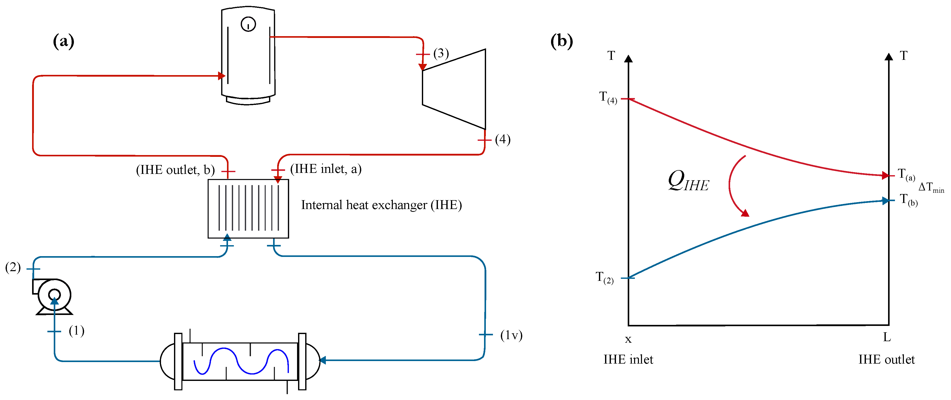
Figure 2.
Depiction of a reversible expansion of an ORC from a saturated condition in the temperature vs. entropy projection for an isentropic working fluid (n-butane is modelled with PC-SAFT). (a) Basic ORC. (b) ORC with an IHE.
Figure 2.
Depiction of a reversible expansion of an ORC from a saturated condition in the temperature vs. entropy projection for an isentropic working fluid (n-butane is modelled with PC-SAFT). (a) Basic ORC. (b) ORC with an IHE.
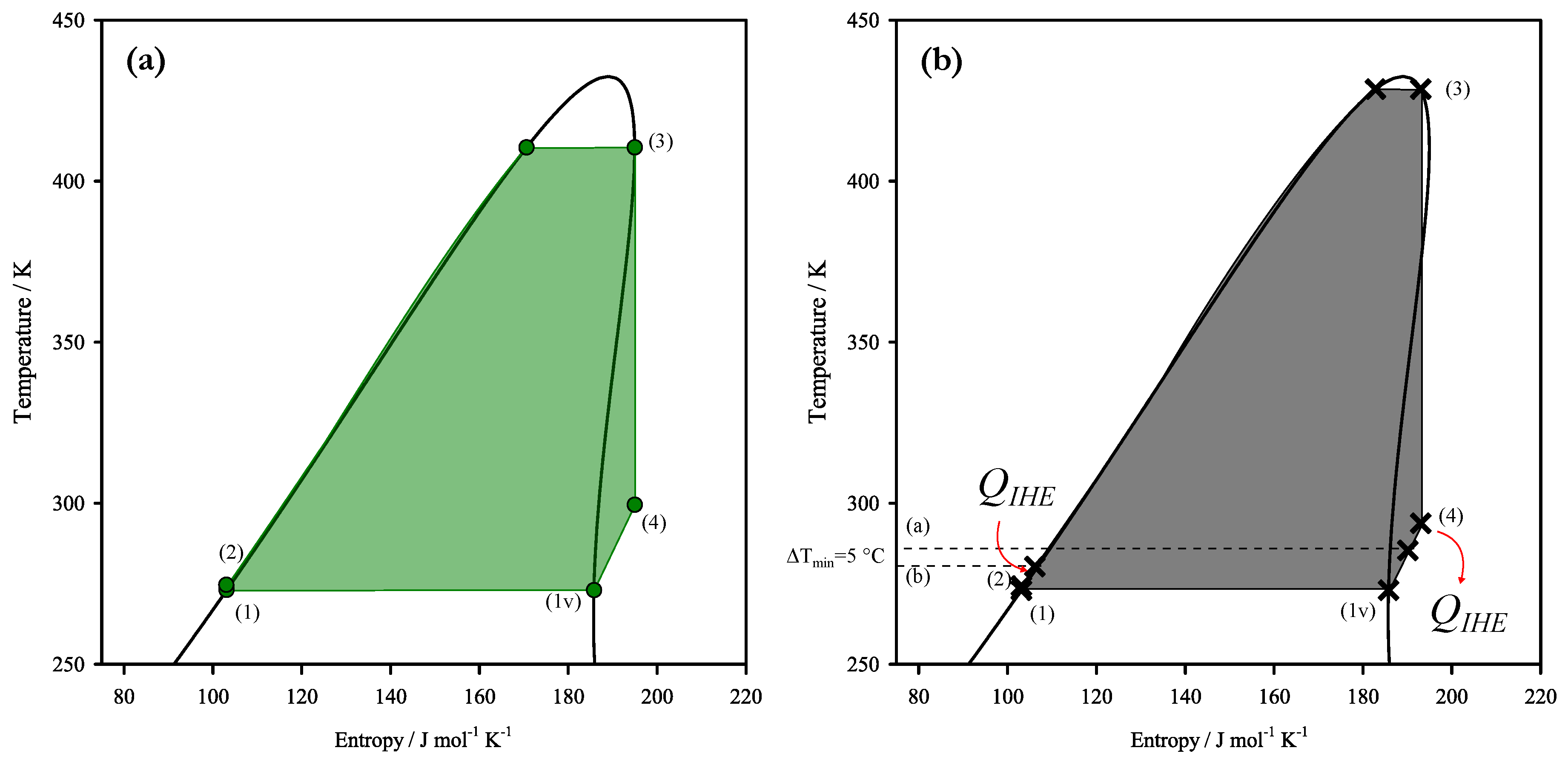
Figure 3.
-function in crimson lines, and -function in blue lines vs. heat capacities of the ideal gas, , as predicted by the van der Waals EOS. Moreover, the expansion regions of the -function and -function are depicted (dry and wet).
Figure 3.
-function in crimson lines, and -function in blue lines vs. heat capacities of the ideal gas, , as predicted by the van der Waals EOS. Moreover, the expansion regions of the -function and -function are depicted (dry and wet).
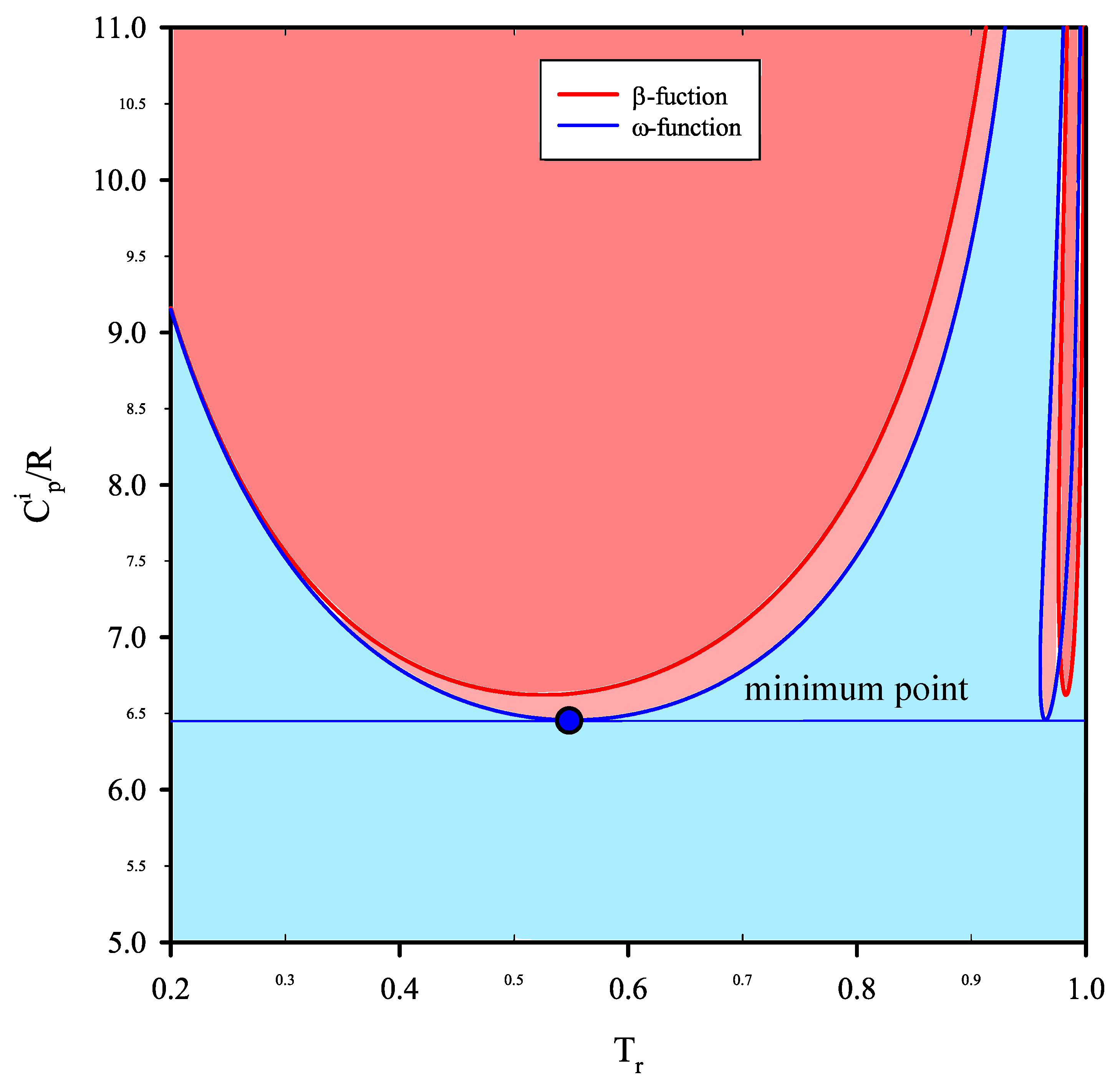
Figure 4.
Schematic representation of an ORC in the temperature vs. entropy projection for a vdW working fluid (=8.0). (a) Graphical representations of ORCs obtained using both the maximum-efficiency equation (crimson points) and the maximum-net-power-output equation (blue points). (b) Graphical representations of ORCs obtained from the fixed condenser temperature and the maximum-entropy point (green points), and from the maximum-efficiency equation, considering an ORC with an IHE (cross points).
Figure 4.
Schematic representation of an ORC in the temperature vs. entropy projection for a vdW working fluid (=8.0). (a) Graphical representations of ORCs obtained using both the maximum-efficiency equation (crimson points) and the maximum-net-power-output equation (blue points). (b) Graphical representations of ORCs obtained from the fixed condenser temperature and the maximum-entropy point (green points), and from the maximum-efficiency equation, considering an ORC with an IHE (cross points).
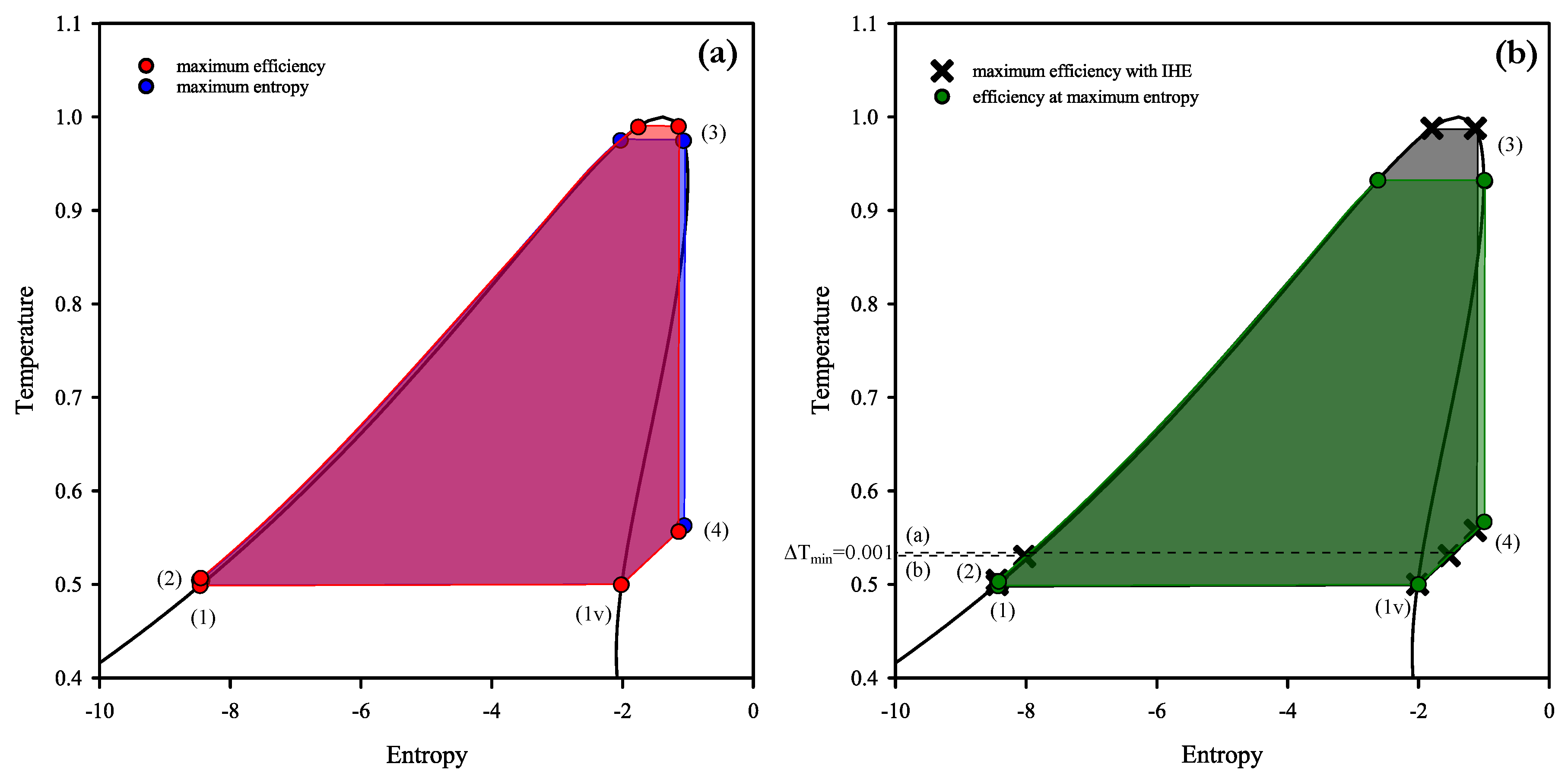
Figure 5.
Efficiency and net power output as functions of boiler temperature for two vdW working fluids. (a) Efficiency for a vdW working fluid represented by =8.0. (b) Net power output for a vdW working fluid, with =8.0. (c) Efficiency for a vdW working fluid represented by =9.0. (d) Net power output for a vdW working fluid, with =9.0.
Figure 5.
Efficiency and net power output as functions of boiler temperature for two vdW working fluids. (a) Efficiency for a vdW working fluid represented by =8.0. (b) Net power output for a vdW working fluid, with =8.0. (c) Efficiency for a vdW working fluid represented by =9.0. (d) Net power output for a vdW working fluid, with =9.0.
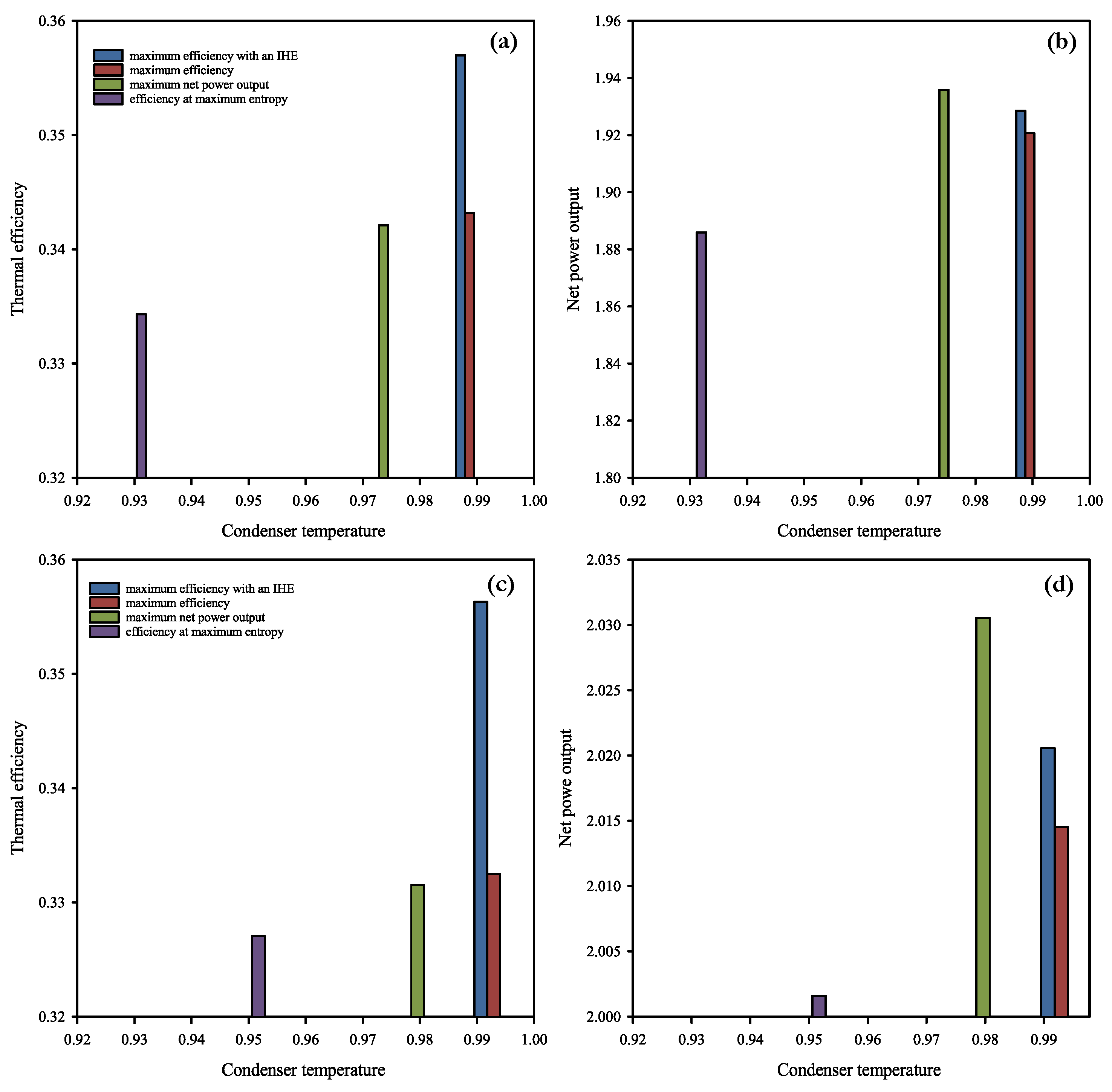
Figure 6.
Boiler temperature and efficiency as functions of the minimum temperature difference in the IHE for two vdW working fluids. (a) Boiler temperature for a vdW working fluid represented by =8.0. (b) Efficiency for a vdW working fluid represented by =8.0. Boiler temperature for a vdW working fluid represented by =9.0. (d) Efficiency for a vdW working fluid represented by =9.0.
Figure 6.
Boiler temperature and efficiency as functions of the minimum temperature difference in the IHE for two vdW working fluids. (a) Boiler temperature for a vdW working fluid represented by =8.0. (b) Efficiency for a vdW working fluid represented by =8.0. Boiler temperature for a vdW working fluid represented by =9.0. (d) Efficiency for a vdW working fluid represented by =9.0.
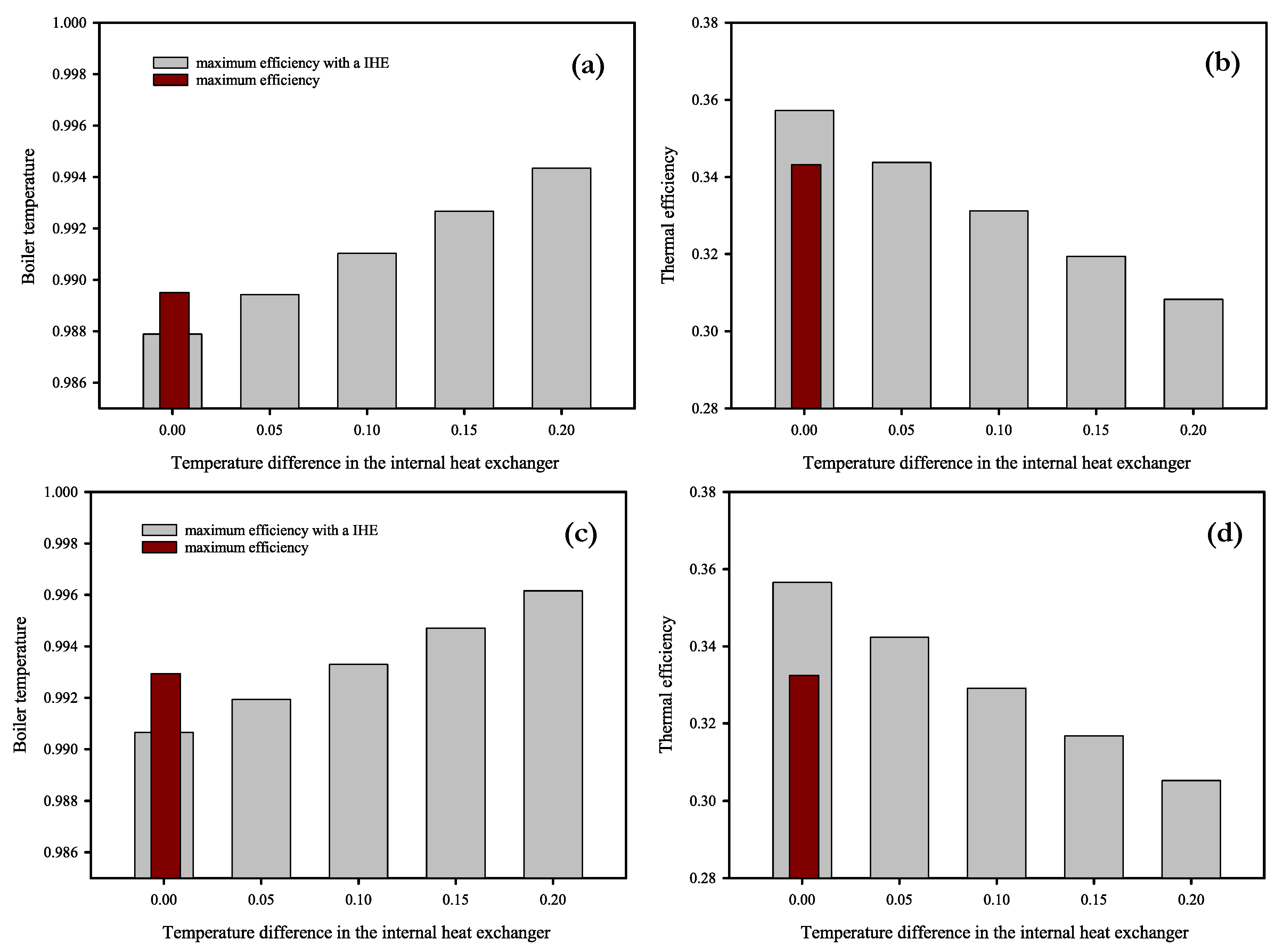
Figure 7.
Variation of the efficiency and the boiler temperature as a function of condenser temperature for several vdW working fluids. vdW working fluids are represented by the blue line (), the black line (), and the crimson line (). The continuous line represents the maximum efficiency obtained with an IHE; the dashed line represents the maximum efficiency obtained without an IHE. (a) Efficiency results. (b) Boiler temperature results.
Figure 7.
Variation of the efficiency and the boiler temperature as a function of condenser temperature for several vdW working fluids. vdW working fluids are represented by the blue line (), the black line (), and the crimson line (). The continuous line represents the maximum efficiency obtained with an IHE; the dashed line represents the maximum efficiency obtained without an IHE. (a) Efficiency results. (b) Boiler temperature results.
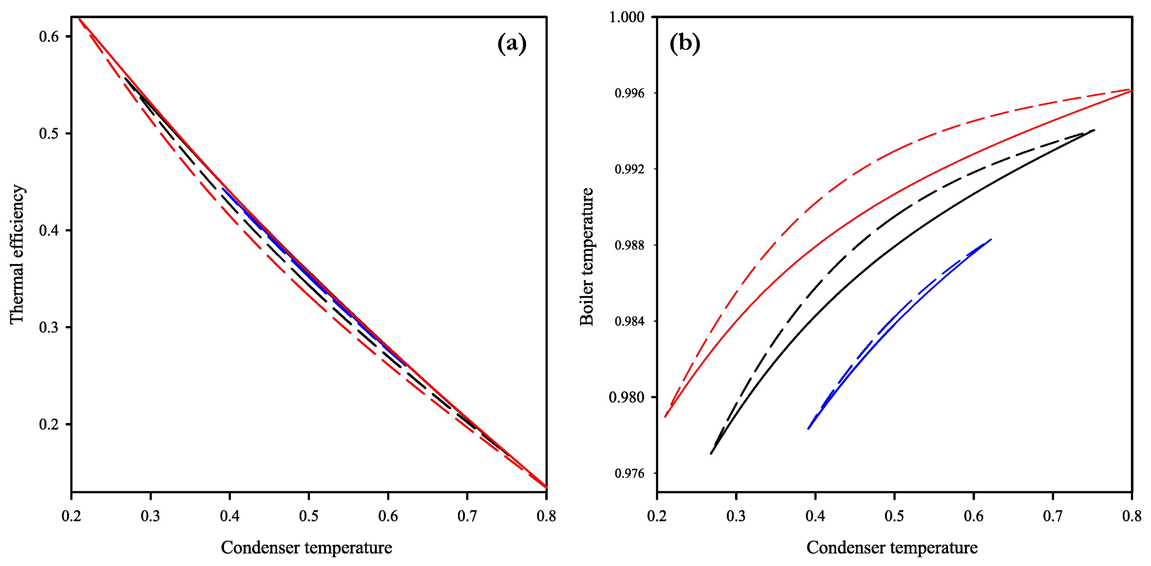
Figure 8.
Relative percentage error as a function of condenser temperature for several vdW working fluids. vdW working fluids are represented by the blue line (), the black line (), and the crimson line (). (a) Efficiency relative percentage error. (b) Boiler temperature relative percentage error.
Figure 8.
Relative percentage error as a function of condenser temperature for several vdW working fluids. vdW working fluids are represented by the blue line (), the black line (), and the crimson line (). (a) Efficiency relative percentage error. (b) Boiler temperature relative percentage error.
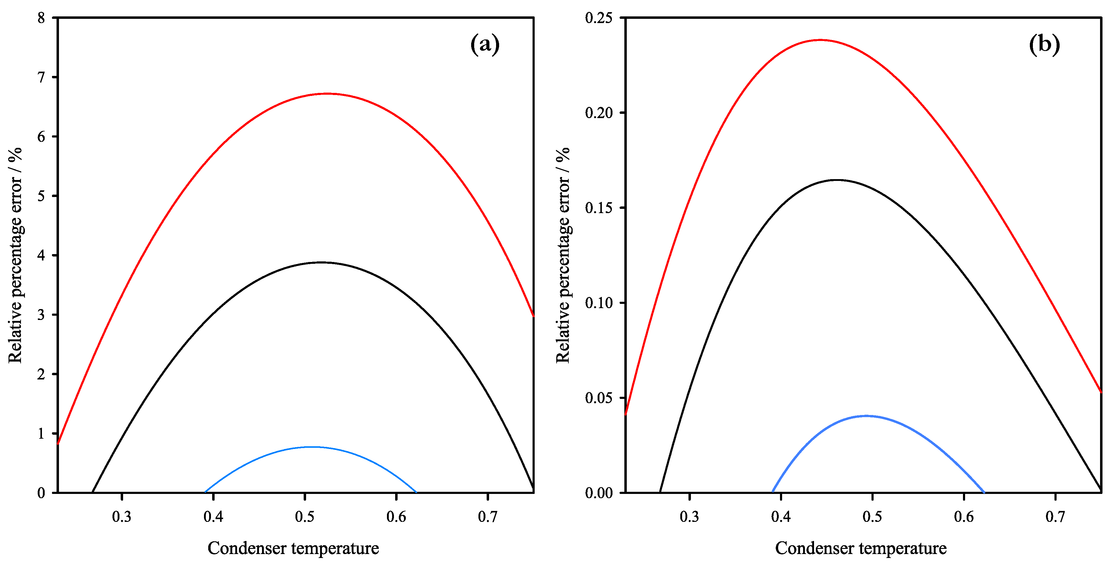
Figure 9.
-function in crimson lines, and -function in blue lines vs. molecular weight, , as predicted by the PC-SAFT EOS. Moreover, the expansion regions of the -function and -function are depicted (dry and wet). In addition, the condenser temperature range analysed in this work for several hydrocarbons is depicted.
Figure 9.
-function in crimson lines, and -function in blue lines vs. molecular weight, , as predicted by the PC-SAFT EOS. Moreover, the expansion regions of the -function and -function are depicted (dry and wet). In addition, the condenser temperature range analysed in this work for several hydrocarbons is depicted.
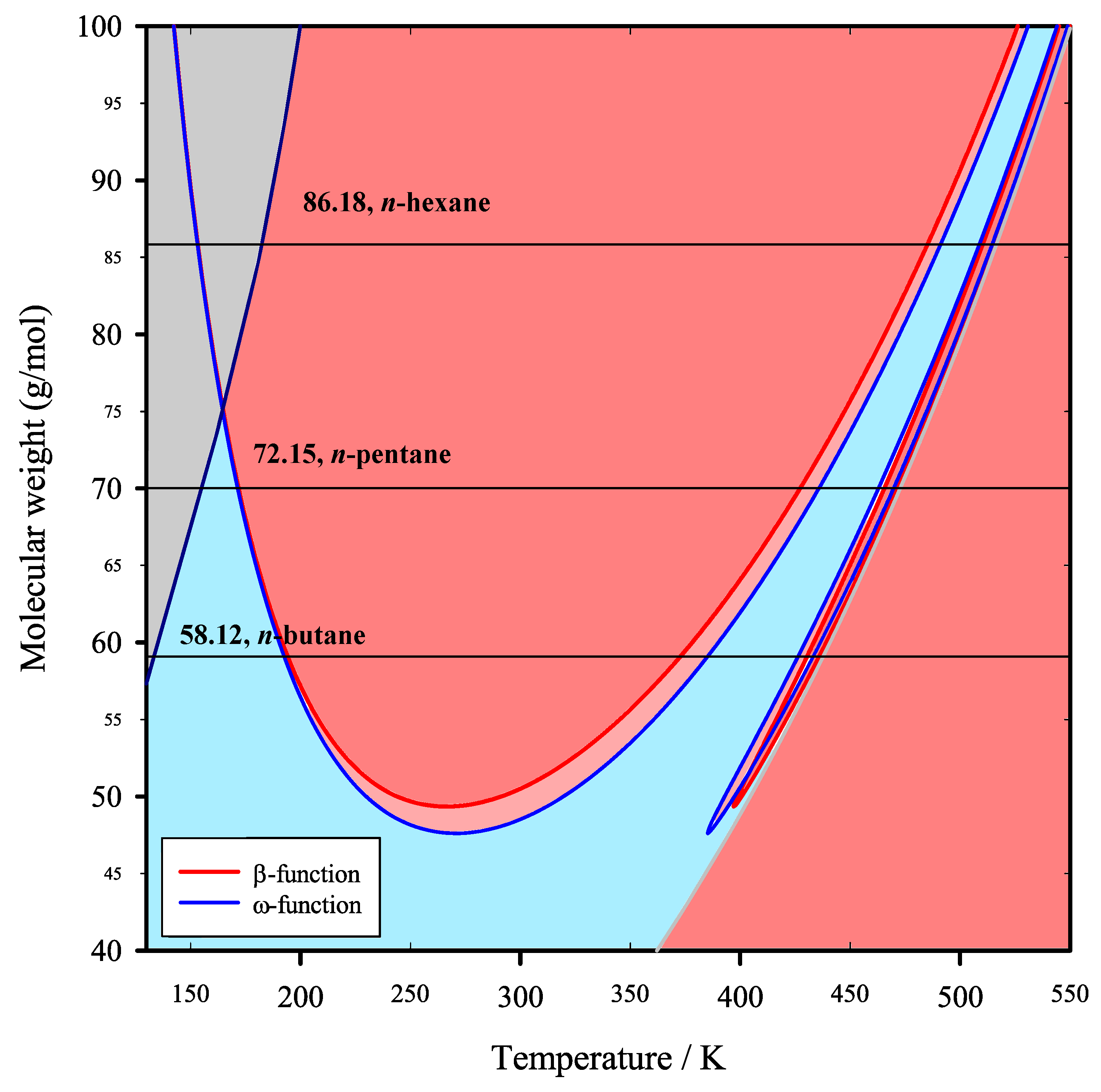
Figure 10.
Efficiency and net power output as functions of boiler temperature for two real working fluids. (a) Efficiency for n-butane. (b) Net power output for n-butane. (c) Efficiency for n-pentane. (d) Net power output for n-pentane.
Figure 10.
Efficiency and net power output as functions of boiler temperature for two real working fluids. (a) Efficiency for n-butane. (b) Net power output for n-butane. (c) Efficiency for n-pentane. (d) Net power output for n-pentane.
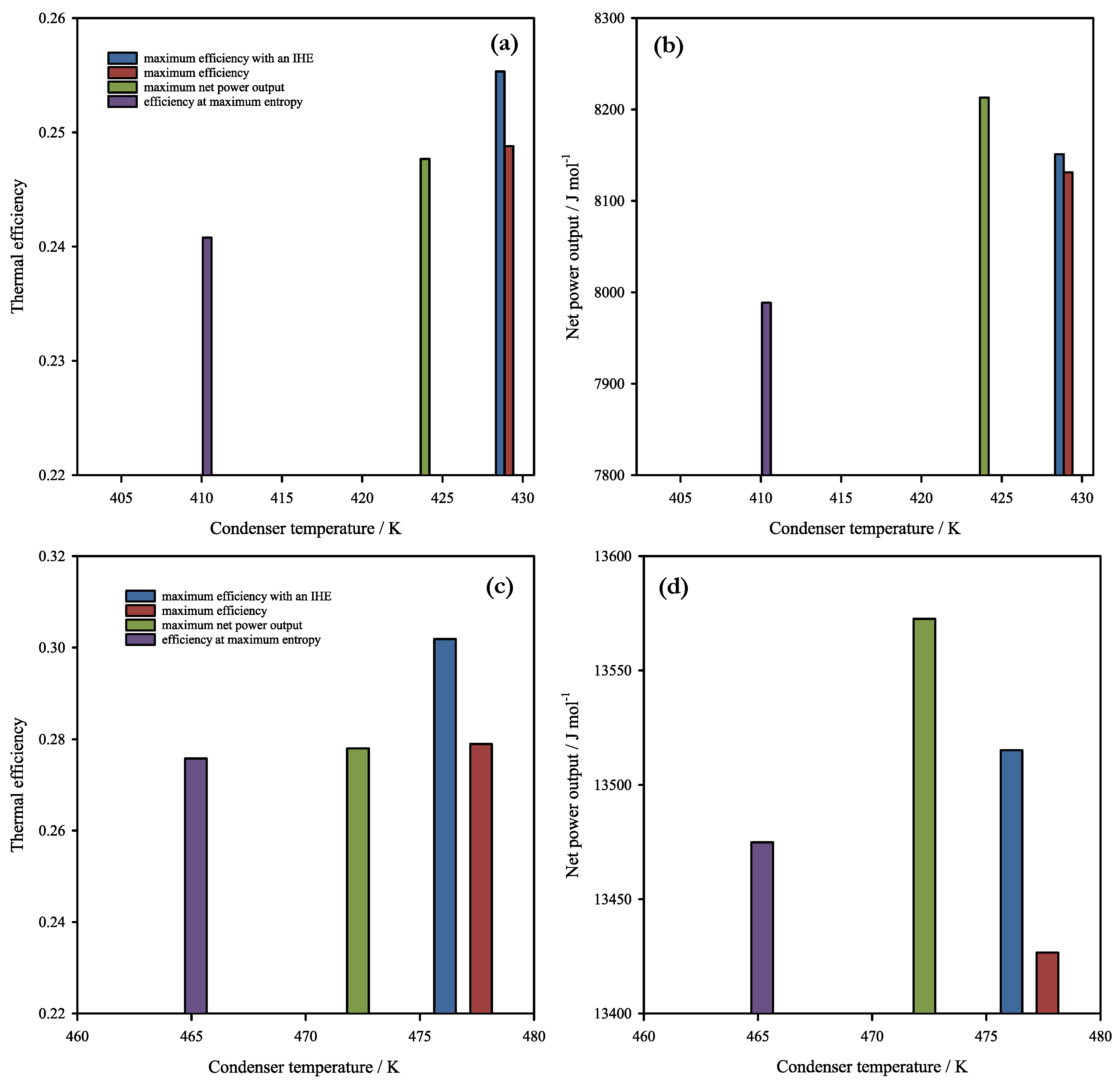
Figure 11.
Boiler temperature and efficiency as functions of the minimum temperature difference in the IHE for two real working fluids. (a) Boiler temperature for a real working fluid represented by n-butane. (b) Efficiency for a real working fluid represented by n-butane. Boiler temperature for a real working fluid represented by n-pentane. (d) Efficiency for a real working fluid represented by n-pentane.
Figure 11.
Boiler temperature and efficiency as functions of the minimum temperature difference in the IHE for two real working fluids. (a) Boiler temperature for a real working fluid represented by n-butane. (b) Efficiency for a real working fluid represented by n-butane. Boiler temperature for a real working fluid represented by n-pentane. (d) Efficiency for a real working fluid represented by n-pentane.
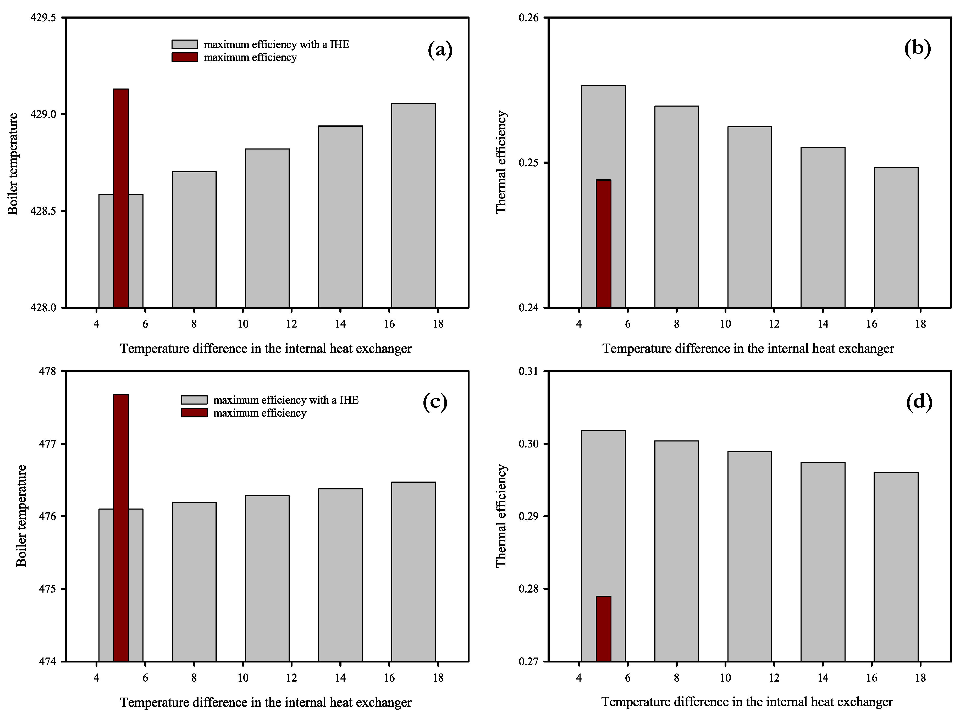
Figure 12.
Efficiency and boiler temperature as functions of condenser temperature for several hydrocarbons as working fluids. The hydrocarbons are represented by the black line (n-butane), the blue line (n-pentane), and the crimson line (n-hexane). In panels (a), (b) and (c), the continuous line represents the results obtained with an IHE and the dashed line those obtained without an IHE. (a) Efficiency. (b) Boiler temperature for n-butane and n-pentane. (c) Boiler temperature for n-pentane and n-hexane.
Figure 12.
Efficiency and boiler temperature as functions of condenser temperature for several hydrocarbons as working fluids. The hydrocarbons are represented by the black line (n-butane), the blue line (n-pentane), and the crimson line (n-hexane). In panels (a), (b) and (c), the continuous line represents the results obtained with an IHE and the dashed line those obtained without an IHE. (a) Efficiency. (b) Boiler temperature for n-butane and n-pentane. (c) Boiler temperature for n-pentane and n-hexane.
Figure 13.
Relative percentage errors as functions of condenser temperature for several hydrocarbons as working fluids. The hydrocarbons are represented by the black line (n-butane), the blue line (n-pentane), and the crimson line (n-hexane). (a) Relative percentage error in efficiency. (b) Relative percentage error in boiler temperature.
Figure 13.
Relative percentage errors as functions of condenser temperature for several hydrocarbons as working fluids. The hydrocarbons are represented by the black line (n-butane), the blue line (n-pentane), and the crimson line (n-hexane). (a) Relative percentage error in efficiency. (b) Relative percentage error in boiler temperature.
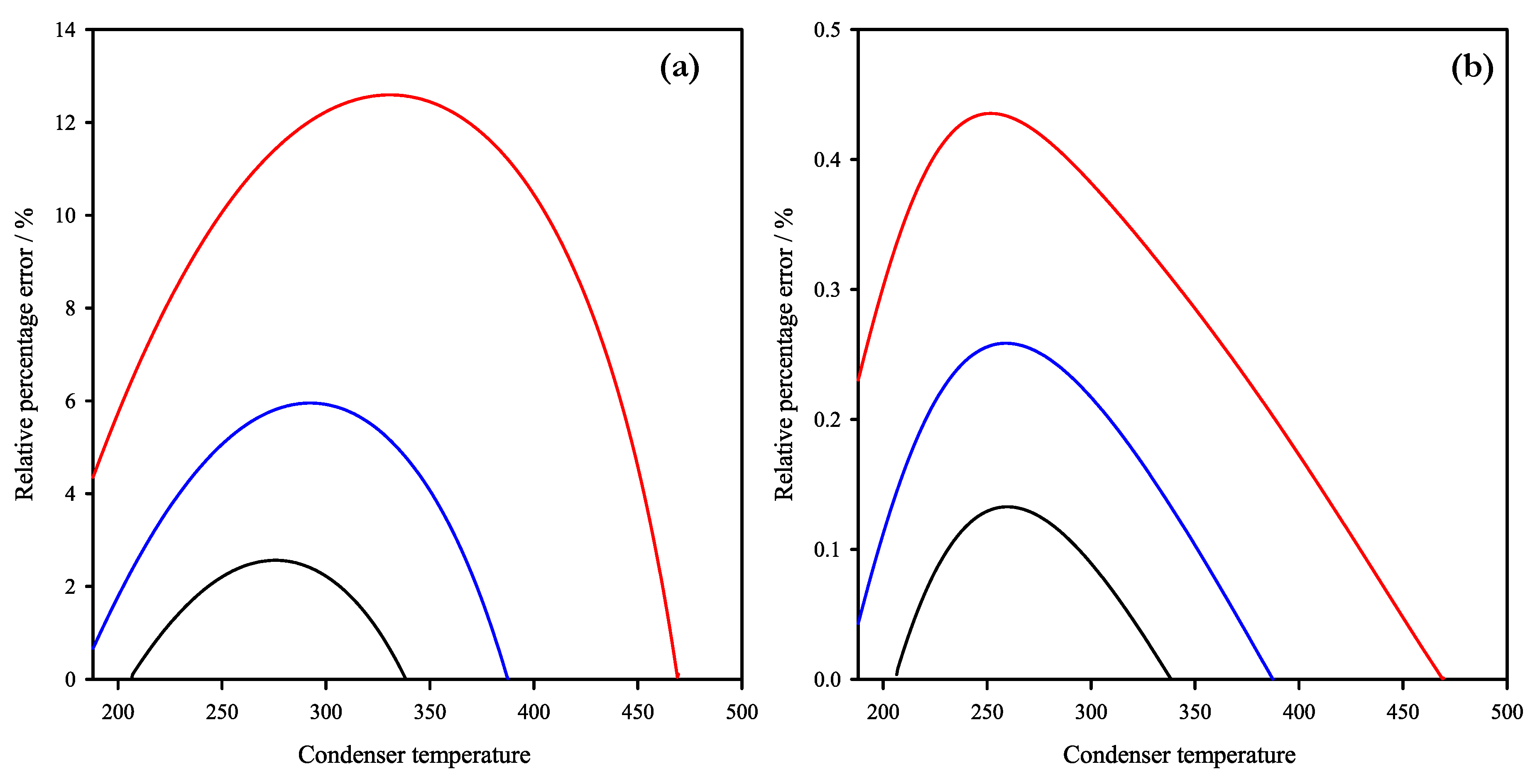
Figure 14.
Efficiency and boiler temperature as functions of condenser temperature for several real working fluids. (a) Thermal efficiency and efficiency relative percentage error. (b) Boiler temperature and boiler temperature relative percentage error.
Figure 14.
Efficiency and boiler temperature as functions of condenser temperature for several real working fluids. (a) Thermal efficiency and efficiency relative percentage error. (b) Boiler temperature and boiler temperature relative percentage error.
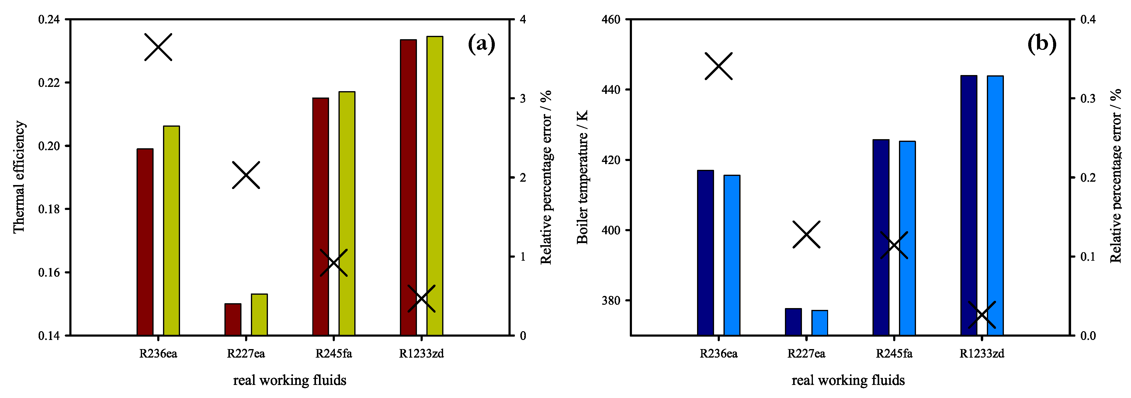

Table 1.
Molecular parameters for the PC-SAFT EOS for the ORC working fluids involved.
| n° | Compound | ASHRAE | m | dev. | Source | ||
|---|---|---|---|---|---|---|---|
| code | Å | K | pph | ||||
| 1 | n-butane | R600 | 2.3316 | 3.7086 | 222.88 | 1.59 | [40] |
| 2 | n-pentane | R601 | 2.6896 | 3.7729 | 231.20 | 0.78 | [40] |
| 3 | n-hexane | - | 3.0576 | 3.7983 | 236.77 | 0.76 | [40] |
| 4 | HFC-236ea | R236ea | 3.6355 | 3.1843 | 180.70 | 0.54 | [26] |
| 5 | HFC-227ea | R227ea | 3.6601 | 3.2621 | 161.06 | 1.09 | [26] |
| 6 | HFC-245fa | R245fa | 3.7492 | 3.1521 | 181.71 | 1.55 | [26] |
| 7 | HCFO-1233zd-E | R1233zd | 3.1368 | 3.3909 | 202.51 | 2.84 | [26] |
Table 2.
Constants for the polynomial correlation of the isobaric heat capacity of the involved ORC working fluids.
Table 2.
Constants for the polynomial correlation of the isobaric heat capacity of the involved ORC working fluids.
| n | ASHRAE | T. range | Source | ||||
|---|---|---|---|---|---|---|---|
| code | K | ||||||
| 1 | R600 | 2.76746 | 3.549044 | –1.0783 | –17384.86 | 200.00-1500.00 | [26] |
| 2 | R601 | 2.80526 | 4.500491 | –1.3805 | –9715.61 | 200.00-1500.00 | [26] |
| 3 | n-hexane | 3.99688 | 5.2209 | –1.61379 | –33903.96 | 200.00-1500.00 | - |
| 4 | R236ea | 9.03210 | 3.180400 | –1.4660 | 199252.44 | 298.15-1000.00 | [26] |
| 5 | R227ea | 11.45250 | 2.994100 | –1.4029 | –250545.45 | 298.15-1000.00 | [26] |
| 6 | R245fa | –18.36220 | 16.266000 | –20.5470 | 157769.57 | 200.00-433.33 | [26] |
| 7 | R1233zd | –3.62707 | 7.990900 | –9.0159 | 20448.70 | 198.15–448.15 | [26] |
Table 3.
Relative percentage error of the saturation boiler temperature and thermal efficiency, and net power output obtained through different operational conditions given by three objective functions and maximum entropy point (vdW working fluids).
Table 3.
Relative percentage error of the saturation boiler temperature and thermal efficiency, and net power output obtained through different operational conditions given by three objective functions and maximum entropy point (vdW working fluids).
| Temperature error/ % | Efficiency error/ % | Net power output error/ % | |||||||
|---|---|---|---|---|---|---|---|---|---|
| 8.0 | 1.5206 | 0.1597 | 5.8124 | 0.3196 | −4.0129 | 2.5870 | 0.7804 | 0.3757 | 2.5761 |
| 9.0 | 1.3403 | 0.2279 | 4.1540 | 0.2931 | −7.1615 | 1.6348 | 0.7882 | 0.2699 | 1.4252 |
Table 4.
Relative percentage error of the saturation boiler temperature and thermal efficiency, and net power output obtained through different operational conditions given by three objective functions and maximum entropy point (real working fluids).
Table 4.
Relative percentage error of the saturation boiler temperature and thermal efficiency, and net power output obtained through different operational conditions given by three objective functions and maximum entropy point (real working fluids).
| Temperature error/ % | Efficiency error/ % | Net power output error/ % | |||||||
|---|---|---|---|---|---|---|---|---|---|
| fluid | |||||||||
| R600 | 1.2166 | 0.1270 | 4.3784 | 0.4496 | −2.6261 | 2.5870 | 0.9970 | 0.7554 | 2.7327 |
| R601 | 1.1282 | 0.3302 | 2.6152 | 0.3402 | −8.2072 | 1.1331 | 1.0756 | 0.4226 | 0.7196 |
Disclaimer/Publisher’s Note: The statements, opinions and data contained in all publications are solely those of the individual author(s) and contributor(s) and not of MDPI and/or the editor(s). MDPI and/or the editor(s) disclaim responsibility for any injury to people or property resulting from any ideas, methods, instructions or products referred to in the content. |
© 2026 by the authors. Licensee MDPI, Basel, Switzerland. This article is an open access article distributed under the terms and conditions of the Creative Commons Attribution (CC BY) license.
Copyright: This open access article is published under a Creative Commons CC BY 4.0 license, which permit the free download, distribution, and reuse, provided that the author and preprint are cited in any reuse.