Preprint
Article

This version is not peer-reviewed.

Chemical Game Theory: Linking Metabolite Diversity, Biosynthetic Architecture, and Realized Payoffs

Submitted:

06 August 2026

Posted:

10 August 2026

You are already at the latest version

Abstract

Plant chemodiversity is generally evaluated through metabolite richness, relative abundance, compositional dissimilarity, and biosynthetic organization. However, these descriptors characterize chemical states without explicitly identifying which metabolites, chemical classes, or biosynthetic pathways gain or lose relative representation during transitions between states. Here, we introduce Chemical Game Theory, an operational framework in which metabolites are treated as elementary chemical strategies, biosynthetic pathways constitute higher-order strategies, and normalized chromatographic abundances define their frequencies within a mixture. Replicator-based equations are used to calculate realized chemical payoffs, which quantify the relative advantage or disadvantage of each strategy during compositional transitions. Shannon diversity describes metabolite-level coexistence, whereas the General Biosynthetic Diversity Index, GBDI, characterizes pathway allocation and intrapathway branching. The framework was applied to previously published GC-MS and GC-FID profiles of essential oils from leaves and four developmental stages of the reproductive organ of Piper mollicomum Kunth, sampled over five months. Leaves exhibited the greatest overall metabolite diversity and biosynthetic architectural complexity, while the reproductive stages followed distinct and temporally variable chemical trajectories. Replicator analysis identified stage-dependent changes in the relative performance of terpenoid, mixed, shikimate-derived, and other biosynthetic strategies. The terpenoid route was consistently favored during specific reproductive-stage transitions, whereas the mixed pathway showed recurrent relative decline. Chemical dominance, Shannon diversity, GBDI, and realized payoff therefore captured distinct but complementary dimensions of chemical organization. Chemical Game Theory provides a quantitative language for interpreting the redistribution of chemical investment across plant compartments and developmental states. In phytochemical and bioprospecting studies, the framework may support the rational selection of plant organs, developmental stages, and collection periods associated with high target-metabolite abundance, emerging chemical strategies, or expanded biosynthetic and structural space.

Keywords: 
;  ;  ;  ;  ;  

1. Introduction

Plants produce chemically complex and dynamic mixtures of specialized metabolites whose composition varies among species, populations, individuals, organs, developmental stages, and environmental conditions. These metabolites participate in defense, signaling, reproduction, stress tolerance, and interactions with other organisms, while also representing a major source of structurally and biologically diverse natural products [1,2,3,4]. Plant chemodiversity should therefore not be regarded as a static inventory of molecular structures, but as a dynamic chemical phenotype generated by the differential allocation of metabolic resources among precursors, enzymes, biosynthetic pathways, and their final products.
Quantitative studies of chemodiversity commonly employ metabolite richness, Shannon and Simpson indices, Hill numbers, evenness, chemical dissimilarities, and metrics incorporating structural or functional distances [4,5,6,7]. These approaches provide valuable information about the number of metabolites, their abundance distribution, and the degree of differentiation among chemical mixtures. However, classical diversity indices generally treat metabolites as independent and exchangeable units, thereby overlooking the nested metabolic relationships that connect chemical products through common precursor pools, catalytic machinery, regulatory controls, and biosynthetic costs. Accordingly, comparable Shannon values can emerge from mixtures characterized by fundamentally different patterns of pathway allocation and internal metabolic branching.
The General Biosynthetic Diversity Index, GBDI, was developed to address this distinction by coupling the abundance of each metabolite with the cumulative abundance of its assigned biosynthetic pathway [8]. GBDI integrates allocation among biosynthetic pathways with diversification occurring within each pathway, thereby distinguishing compound-level diversity from biosynthetic architectural diversity. A mixture dominated by one pathway may still exhibit a relatively high GBDI when that pathway is internally branched into several quantitatively relevant products. Conversely, a mixture containing several pathways may remain architecturally canalized if most chemical abundance is concentrated in a single compound or route. Shannon diversity and GBDI therefore describe complementary properties of chemical organization.
Although these descriptors quantify the structure of a chemical state, they do not directly indicate which chemical components gain or lose relative representation during transitions between states. This distinction is important because chemical dominance and directional advantage are not equivalent. A highly abundant metabolite may remain dominant while already decreasing proportionally, whereas a minor compound or pathway may exhibit rapid relative expansion before becoming quantitatively prominent. Static comparisons can identify compositional differences, but they do not formally quantify the direction and intensity of the redistribution of chemical investment.
Game theory provides a mathematical framework for systems in which the performance of a strategy depends on the composition and behavior of the surrounding system [9,10,11,12]. In evolutionary game theory, strategies do not need to correspond to conscious decisions. They may represent phenotypes, resource-allocation patterns, functional traits, or other alternatives whose relative frequencies change according to their performance. Replicator dynamics formalize this principle by predicting that strategies with performance above the system-wide mean increase in frequency, whereas strategies with below-average performance decline [11,12,13].
However, classical non-cooperative game theory defines a Nash equilibrium as a strategy profile in which no player can improve its payoff through unilateral deviation while the strategies of the other players remain unchanged [14]. The present framework, however, does not attempt to estimate a Nash equilibrium among metabolites. Instead, Chemical Game Theory adopts the relative-performance principle underlying evolutionary game dynamics, particularly the replicator equation, in which the frequency of a strategy changes according to the difference between its performance and the mean performance of the population [15,16]. In the proposed chemical translation, metabolites are not regarded as autonomous biological agents but as chemical strategies whose proportional representation reflects the allocation of biosynthetic investment within a compositional system. The continuous fitness-difference term of the replicator equation is operationalized for discrete chromatographic observations through the logarithmic change in relative metabolite abundance between consecutive biological states. The realized relative payoff of each metabolite is subsequently obtained by subtracting the abundance-weighted mean chemical change from its individual logarithmic change. Thus, the framework quantifies whether a chemical strategy gained or lost proportional representation relative to the overall reorganization of the mixture, allowing ontogenetic stages, plant organs, environmental conditions, or other ordered biological states to be compared using GC–MS or LC–MS data.
Game-theoretical models have been applied to plant competition, resource acquisition, defense allocation, herbivory tolerance, allelopathy, and chemical communication [17,18,19,20,21]. Game theory has also contributed to theoretical discussions concerning the evolution and maintenance of plant chemodiversity, particularly through frequency-dependent interactions among defended and undefended plants or among plants, herbivores, and competing organisms [22,23]. In most of these models, however, the strategies correspond to organisms, phenotypes, or defense-investment levels. Chromatographically measured metabolites and biosynthetic pathways have rarely been operationalized as frequency-distributed strategies whose directional performance can be calculated directly from empirical chemical compositions.
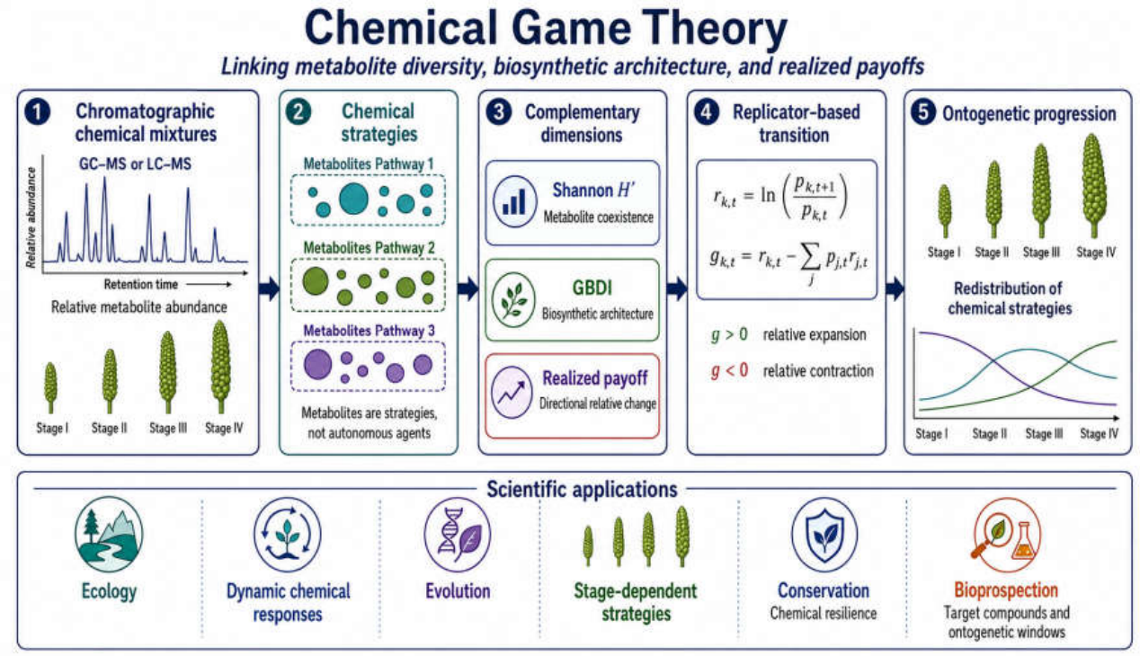
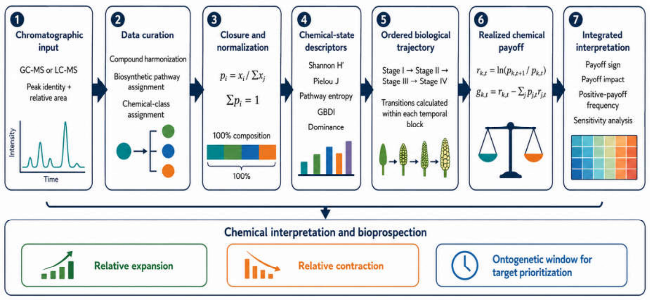
Here, we introduce Chemical Game Theory (Figure 1 and Figure 2) as an operational framework for interpreting dynamic plant chemodiversity. Individual metabolites are represented as elementary chemical strategies, while chemical classes and biosynthetic pathways constitute progressively higher hierarchical levels. Relative chromatographic abundances define the frequencies of these strategies within a mixture. Changes between consecutive chemical states are evaluated using a replicator-based formulation that produces realized chemical payoffs. A positive payoff indicates that a strategy gained proportional representation relative to the mean change of the chemical system, whereas a negative payoff indicates relative decline.
The term chemical strategy is used in an operational and mathematical sense. Metabolites are not considered autonomous agents, and their changes are not interpreted as molecular reproduction or conscious decision-making. Instead, their relative abundances are treated as observable outcomes of metabolic allocation, precursor availability, enzymatic regulation, transport, storage, volatilization, and degradation. Similarly, a realized chemical payoff describes the relative performance observed during a transition but does not independently demonstrate that one metabolite caused the increase or suppression of another.
The proposed framework separates four complementary dimensions of chemical organization. Chemical dominance identifies the most abundant compounds or pathways. Shannon diversity describes metabolite-level coexistence and abundance distribution. GBDI characterizes the abundance-weighted organization of metabolites within and among biosynthetic pathways. Realized chemical payoff quantifies the direction and intensity with which a strategy changes between consecutive chemical states. These dimensions may be related, but they are not interchangeable. A mixture may exhibit high GBDI and low Shannon diversity, or a rare pathway may present a positive payoff without becoming quantitatively dominant.
Developmental and organ-specific chemical variation provides a particularly suitable context for demonstrating the framework. Plant organs differ in physiological function, tissue value, resource availability, storage capacity, and exposure to biotic and abiotic pressures [24,25,26]. Reproductive development may involve changes in enzymatic activity, precursor allocation, oxidation, volatilization, and the relative importance of defensive or signaling compounds. Consequently, successive stages of an organ may occupy distinct regions of compositional and biosynthetic space.
From a phytochemical perspective, these differences are directly relevant to natural-product discovery. Bioprospecting strategies frequently prioritize taxonomic identity, traditional use, preliminary biological activity, or the abundance of known compounds [27,28,29,30]. However, the organ and developmental stage selected for extraction may strongly influence the probability of obtaining a target metabolite, detecting minor compounds, or accessing a broader biosynthetic space. Developmental variation should therefore not be treated only as analytical noise. It may provide a rational criterion for selecting plant material.
Chemical Game Theory introduces an additional distinction for bioprospecting. A plant compartment may be selected because it already contains a high concentration of a target compound, which can be defined as a target-yield window. Alternatively, a transition may be selected because a target compound or biosynthetic pathway has begun to gain proportional representation, even before reaching dominance. This second condition can be defined as a strategic-emergence window. The first favors extraction yield, whereas the second may help identify developmental periods of active chemical reorganization and expanded probability of detecting emerging or minor metabolites.
The framework may also support sample prioritization when combined with untargeted chemical profiling, early recognition of known constituents, molecular-network analysis, and bioactivity screening. High GBDI does not necessarily predict biological activity or structural novelty. Nevertheless, it may identify samples with expanded pathway participation or substantial intrapathway branching. Realized payoffs can complement this information by revealing which compounds or pathways are actively gaining representation. Together, these descriptors may guide the rational allocation of analytical effort toward samples with high target abundance, broader chemical space, or informative metabolic transitions.
As proof of concept, we applied Chemical Game Theory to previously published essential-oil data from Piper mollicomum Kunth [31]. The dataset includes leaves and four developmental stages of the reproductive organ sampled monthly from September to January. Essential oils were characterized by GC-MS and quantified by GC-FID. This design provides two complementary levels of comparison. Leaves serve as a vegetative reference for evaluating compartment-specific chemodiversity, while stages I–IV constitute an ordered reproductive trajectory that can be evaluated independently within each monthly block.
The biosynthetic classification used in the present analysis followed the precursor origin of the detected volatile constituents. Terpenoids were assigned to the terpene pathway, benzyl benzoate was assigned to the shikimate pathway, and eupatoriochromene was treated as a mixed-pathway metabolite. This classification is particularly informative because eupatoriochromene can contribute substantially to some reproductive-stage oils, whereas benzyl benzoate represents a less abundant but biosynthetically distinct strategy. The framework can therefore evaluate not only dominant terpenoid allocation but also the directional behavior of minor and mixed biosynthetic components.
Accordingly, the objectives of this study were: (i) to formulate a game-theoretical representation of chromatographic chemical mixtures; (ii) to derive realized chemical payoffs from changes in relative metabolite abundance; (iii) to integrate payoff analysis with Shannon diversity and GBDI; (iv) to compare the chemodiversity and biosynthetic architecture of leaves and reproductive stages of P. mollicomum; (v) to evaluate stage transitions independently across five monthly blocks; and (vi) to discuss the application of Chemical Game Theory to the rational selection of organs, developmental stages, and collection periods for phytochemical investigation and bioprospection.

2. Results and Discussion

2.1. Construction of the Chemical Game from Ontogenetic Essential-Oil Profiles

The essential-oil dataset of Piper mollicomum provided an appropriate empirical system for demonstrating the proposed Chemical Game Theory framework because it combined chemical composition, biosynthetic organization, organ differentiation, and an ordered reproductive-development sequence. The original dataset comprised essential oils obtained from leaves and four developmental stages of the reproductive organ, sampled monthly from September 2020 to January 2021 [31]. See Supplementary File S1.
Each chromatographic profile was treated as a finite chemical system composed of S detected metabolites. The relative chromatographic abundance of metabolite i , denoted p i , was interpreted as its realized allocation within the mixture. This interpretation recognizes that normalized chromatographic profiles are compositional: the components are constrained by a constant sum and, consequently, cannot vary independently [32,33,34].
For each chemical state, the relative abundances were normalized according to (Figure S1):
p i = x i j = 1 S x j
and therefore:
i = 1 S p i = 1
where x i is the chromatographic abundance originally reported for metabolite i .
Calculations were performed using the complete individual profiles reported as “% in 1” in Supplementary Table S3 of the original study [31]. These profiles were selected because they constituted internally reconcilable compositional vectors. The arithmetic averages reported for selected major constituents in other supplementary tables were retained for descriptive comparisons but were not used as closed input vectors because they did not include every detected constituent.
The metabolites were analyzed at three nested strategic levels:
  • individual metabolites;
  • chemical classes;
  • biosynthetic pathways.
This hierarchical organization recognizes that plant specialized metabolism can be evaluated both through the behavior of individual products and through the broader precursor-generating and enzymatic systems responsible for their formation [23,24,25,26].
The four developmental stages constituted the ordered chemical-game trajectory:
Stage   I Stage   II Stage   III Stage   IV
Leaves were treated as a vegetative reference compartment and not as an ontogenetic Stage 0. A leaf-to-reproductive-organ transition would combine two distinct biological effects, organ identity and developmental progression. Consequently, realized payoffs were calculated only between adjacent reproductive stages within the same monthly block. Leaves were compared with the reproductive stages using diversity, dominance, and biosynthetic-architecture descriptors (Tables S1 and S2).
In classical game theory, payoff describes an outcome associated with a strategy under a defined interaction structure. Evolutionary game theory extends this reasoning to changes in the relative frequencies of strategies within a population [9,10,11,12,13]. In the present framework, metabolites were not regarded as autonomous agents capable of making decisions. Instead, game theory was used as a mathematical language for describing the redistribution of relative chemical investment within a closed metabolomic system.
Accordingly, the terms “chemical player”, “chemical strategy”, and “realized chemical payoff” constitute operational analogies. The realized chemical payoff does not represent biological fitness in the strict Darwinian sense. It measures whether the representation of a metabolite, chemical class, or biosynthetic pathway increased or decreased relative to the abundance-weighted chemical background during a defined transition. This application of game-theoretical reasoning to chromatographic chemodiversity is new and proposed in this article (Tables S1 and S2).

2.2. Vegetative and Reproductive Compartments Occupied Distinct Regions of Chemical Diversity Space

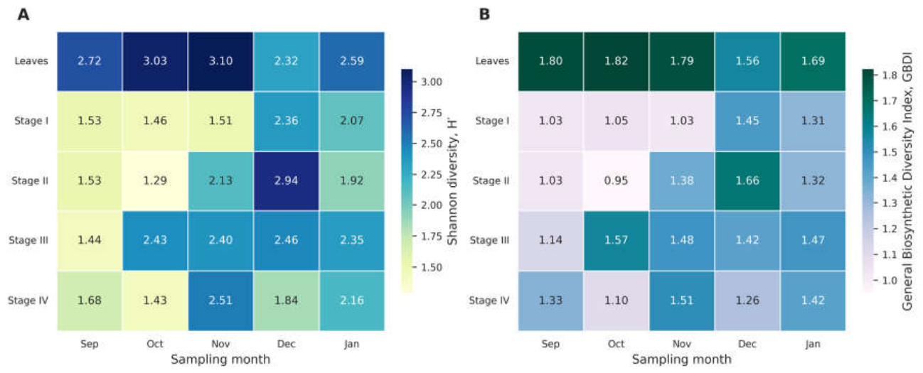
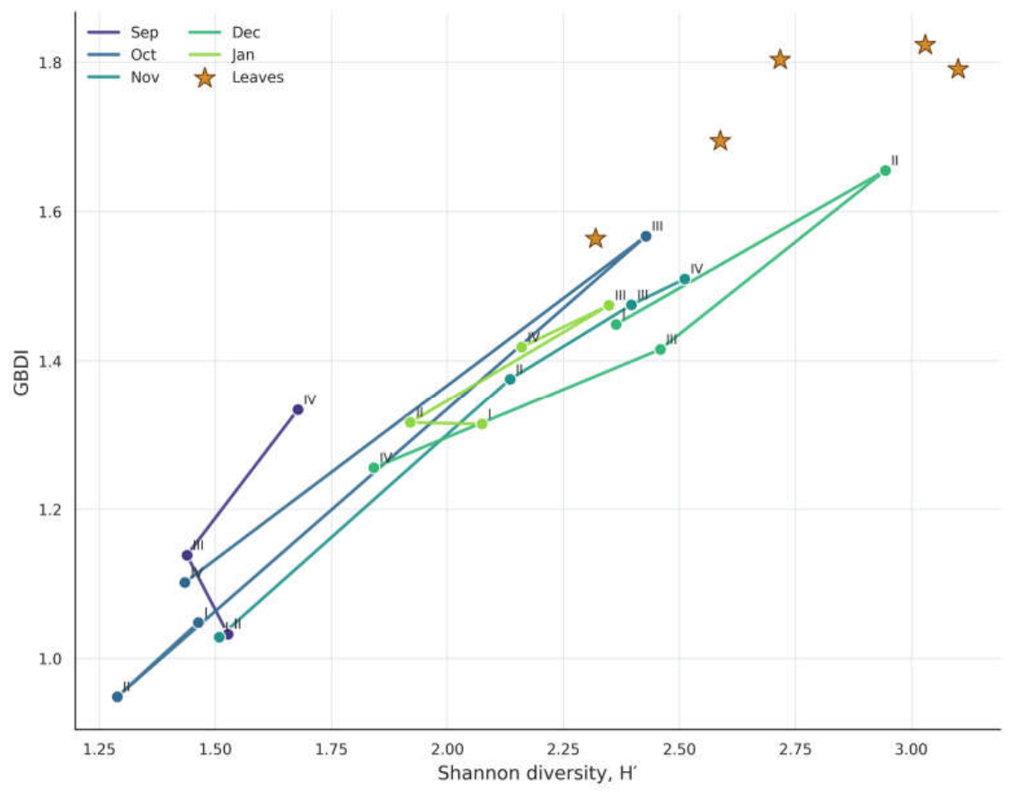
Leaves showed the highest mean Shannon diversity and GBDI among the evaluated compartments, with H ' = 2.751 ± 0.322 and GBDI = 1.735 ± 0.108 , respectively (Table 1 and Tables 1 and S1; Figure 3). Mean Pielou evenness was also relatively high in leaves, J = 0.748 , while the mean proportional abundance of the dominant metabolite was 0.280. Shannon diversity measures the uncertainty associated with the identity of a randomly selected component and is influenced by both richness and abundance distribution [2,3,4,5]. GBDI, in contrast, incorporates both metabolite-level abundance and the organization of those metabolites among biosynthetic pathways [8]. The two indices therefore provide complementary descriptions of chemical diversity.
Reproductive Stage I presented the lowest mean Shannon diversity and GBDI, 1.787 ± 0.408 and 1.175 ± 0.195 , respectively. Stage II exhibited a moderate increase in both indices. This tendency continued at Stage III, which showed the highest mean Shannon diversity and GBDI among the reproductive stages, 2.214 ± 0.435 and 1.414 ± 0.163 , respectively.
The transition from Stage III to Stage IV was accompanied by reductions in Shannon diversity and GBDI. Mean Shannon diversity declined from 2.214 to 1.925, and mean GBDI declined from 1.414 to 1.324. Simultaneously, the mean abundance of the dominant metabolite increased from 0.356 to 0.407. Together, these results indicate that late reproductive development was associated, on average, with greater concentration of chemical abundance around a smaller subset of quantitatively dominant metabolites.
Values are means ± standard deviations calculated from five monthly blocks. Pielou evenness and dominance variables are presented as monthly means. p m a x is the abundance of the dominant metabolite, and P m a x is the abundance of the dominant biosynthetic pathway. Friedman tests compared leaves and the four reproductive stages using month as the temporal block. Bold values indicate p < 0.05. Leaves were treated as a vegetative reference and not as an ontogenetic Stage 0.
The blocked Friedman analysis detected differences among compartments for GBDI ( χ 2 = 10.72 , d f = 4 , p = 0.0299 ), pathway entropy ( χ 2 = 17.12 , p = 0.0018 ), and dominant-pathway abundance ( χ 2 = 17.12 , p = 0.0018 ). Shannon diversity did not differ significantly in the omnibus analysis ( p = 0.1933 ), despite its higher mean in leaves.
No pairwise Wilcoxon comparison remained significant after Holm correction. This absence of significant post hoc contrasts should not be interpreted as evidence that the compartments were chemically equivalent. With only five temporal blocks, the paired tests had limited power, and the adjusted p -values were conservative. The omnibus results should therefore be regarded as exploratory evidence for compartment-dependent chemical organization (Supplementary File S1).

2.2. Shannon Diversity, Pathway Entropy, and GBDI Represented Different Properties of the Chemical System

Although Shannon diversity and GBDI showed broadly similar trends, they did not measure the same chemical property. Shannon diversity was determined by the distribution of abundance among individual metabolites, independently of biosynthetic origin [2,3,4,5]. GBDI additionally considered the relationship between each metabolite and the total abundance of its assigned biosynthetic pathway [8].
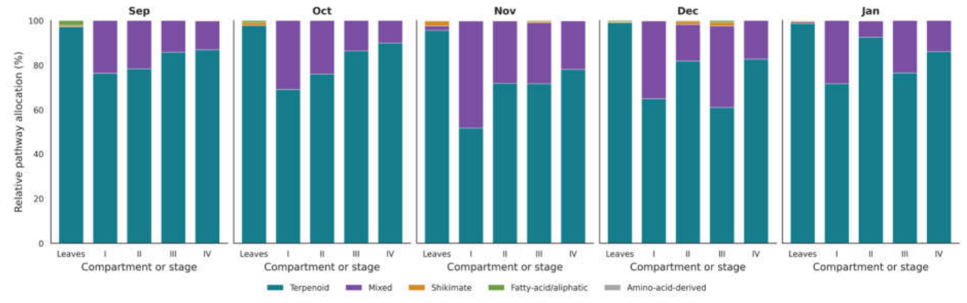
This distinction was particularly evident in leaves. Leaves exhibited the highest mean Shannon diversity and GBDI, although approximately 97.7% of their normalized chemical abundance belonged to the terpenoid pathway. Consequently, leaves displayed very low pathway entropy, H p a t h = 0.125 , and high dominant-pathway abundance, P m a x = 0.977 .
The high GBDI of leaves did not, therefore, result from an even distribution among several biosynthetic pathways. Instead, it reflected extensive chemical diversification within the quantitatively dominant terpenoid pathway. Plant terpenoid metabolism can produce many structurally distinct compounds from a relatively restricted set of precursor pools through the action of terpene synthases and subsequent modifying enzymes [23,24,25,26]. The leaf profile is consistent with this type of intrapathway diversification.
Reproductive stages exhibited a different organization. Their total Shannon diversity and GBDI were generally lower than those of leaves, but their pathway entropy was substantially higher. In Stage I, the terpenoid pathway represented a mean of 66.83% of the normalized profile, while the mixed pathway, represented principally by eupatoriochromene, accounted for 33.07% (Table 2, Figure 4). This more balanced allocation generated the highest mean pathway entropy among the evaluated compartments.
The comparison demonstrates that a chemically diverse system is not necessarily balanced among biosynthetic pathways. Two distinct architectures can therefore be recognized:
  • ✓ high compound diversity associated with extensive branching within one dominant pathway;
  • ✓ greater balance among pathways associated with lower total compound diversity.
Pathway entropy can distinguish these architectures, while GBDI integrates metabolite diversity and biosynthetic organization into a single compound-sensitive descriptor [8]. For this reason, GBDI should not be interpreted as equivalent to pathway evenness.
Values are means ± standard deviations across the five monthly blocks. Eupatoriochromene was assigned to a mixed biosynthetic pathway, and benzyl benzoate was assigned to the shikimate pathway. Other pathways comprised fatty-acid/aliphatic and amino-acid-derived metabolites. Percentages were calculated from normalized individual chemical profiles.

2.3. Ontogenetic Chemical Reorganization Was Dynamic Rather Than Strictly Monotonic

The reproductive trajectory did not follow a single monotonic pattern shared by every monthly block (Figure 5). Stage III represented the highest mean of reproductive diversity, but the magnitude and direction of the transitions varied among months.
Ontogenetic variation in plant-specialized metabolism is expected because metabolite production, storage, conversion, and emission can change with tissue differentiation, organ maturation, resource allocation, and developmental regulation [23,24,25,26]. Environmental and seasonal conditions may additionally modulate the chemical phenotype expressed at a given developmental stage.
Stage I generally represented a chemically concentrated initial reproductive state. Its mean dominant-metabolite abundance was 0.388, and it presented the lowest Shannon diversity of the reproductive trajectory. Stage II was associated with a partial redistribution of abundance and greater evenness, with mean Pielou evenness increasing from 0.701 to 0.764.
Stage III represented the broadest mean of reproductive chemical state. Its higher Shannon diversity and GBDI indicate that a larger collection of metabolites attained quantitatively relevant abundances during this intermediate developmental phase. Stage IV showed renewed chemical concentration, particularly around quantitatively dominant terpenoids.
The absence of a strictly monotonic trajectory does not invalidate the ordered-game representation. Each transition defines a separate chemical context. In game-theoretical terms, the outcome associated with a strategy depends on the state of the system and the frequencies of the other strategies [9,10,11,12,13]. Similarly, the realized chemical payoff of a metabolite can be positive during one ontogenetic transition and negative during another.
A positive payoff should not be interpreted as a prediction that the metabolite will continue increasing in all subsequent stages. Instead, it identifies a transition-specific interval in which the metabolite increased relative to the chemical background. Reversals in payoff sign can therefore reveal transient biosynthetic windows.

2.4. Realized Chemical Payoffs Quantified Directional Redistribution

For each strategy k , corresponding to metabolite, chemical class, or biosynthetic pathway, compositional log growth was calculated as:
r k , t = l n p k , t + 1 p k , t
Log-ratio transformations are appropriate for compositional systems because they express changes in one component relative to other components rather than treating proportions as independent variables [32,33,34].
The realized chemical payoff was defined as:
g k , t = r k , t j p j , t r j , t
The second term is the abundance-weighted mean log growth of the chemical system. Centering the log growth of each strategy relative to this background follows the relative-performance logic underlying evolutionary and replicator game models [9,10,11,12,13]. However, its application as a realized payoff for chromatographic components is proposed in this study.
Under this definition:
g k , t > 0 indicates relative chemical expansion;
g k , t < 0 indicates relative chemical contraction;
g k , t 0 indicates change like the abundance-weighted chemical background.
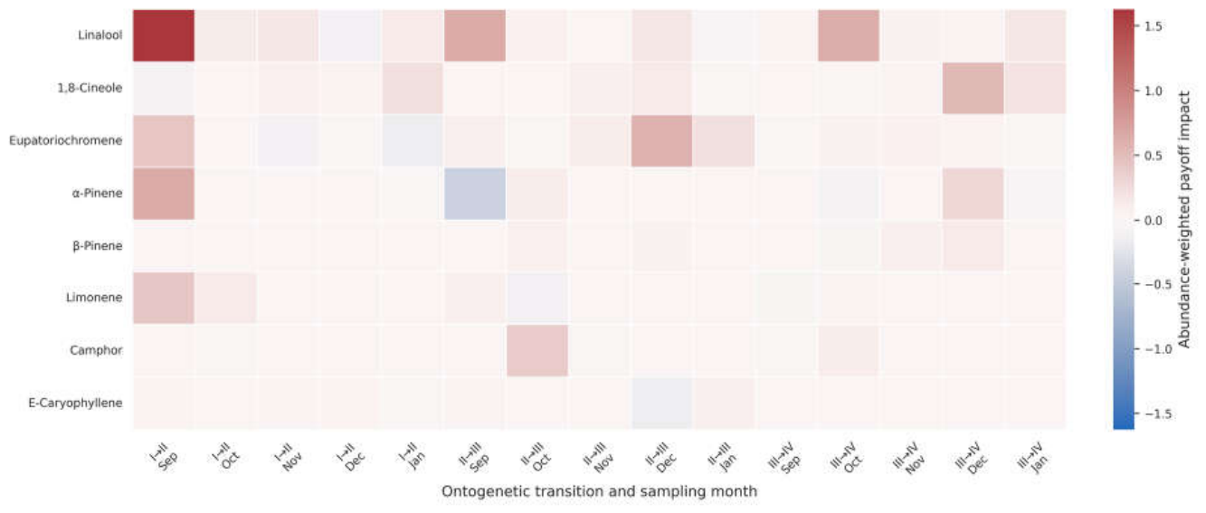
These values are context dependent. A positive chemical payoff is not an intrinsic property of a metabolite and does not imply molecular agency, intentional competition, or Darwinian fitness. It indicates that the metabolite or aggregated chemical strategy gained relative representation during a defined transition (Table 3 and Tables 3 and S4).

2.4.1. Stage I→Stage II

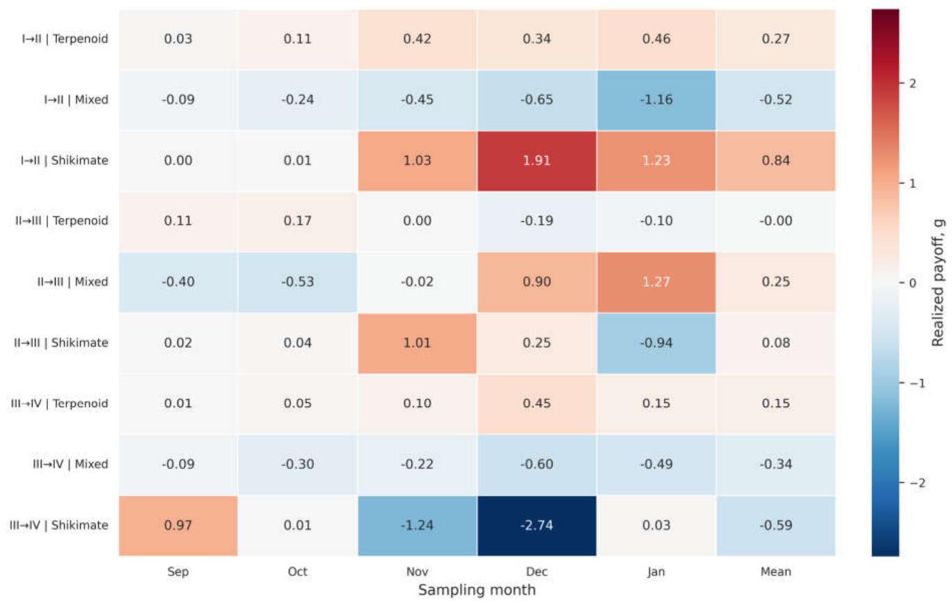
The Stage I→Stage II transition showed a clear redistribution between the terpenoid and mixed pathways. The terpenoid pathway exhibited a positive mean payoff of 0.269 ± 0.191 and was positive in all five monthly blocks. Its mean abundance-weighted impact was also strongly positive, 0.196.
In contrast, the mixed pathway had a consistently negative payoff of 0.518 ± 0.418 , with negative values in all five months. Because this pathway represented approximately one-third of the Stage I profile, its negative payoff produced a substantial mean impact of 0.126 .
This transition can therefore be interpreted as a reproducible relative reallocation from a mixed-pathway-rich initial stage toward greater terpenoid representation. Eupatoriochromene remained an important constituent, but its proportional contribution declined relative to the chemical background.
The shikimate pathway exhibited the highest numerical mean payoff, 0.837 ± 0.824 , and was positive in all months. Nevertheless, its impact was only 0.0037 because the pathway occupied a very small fraction of the mixture. This result demonstrates that payoff magnitude and quantitative influence are not equivalent.

2.4.2. Stage II→Stage III

The Stage II→Stage III transition was comparatively neutral at the pathway level. The terpenoid pathway had a mean payoff close to zero, 0.002 ± 0.146 , and was positive in three of the five monthly blocks.
The mixed pathway had a positive mean payoff of 0.246 but a large standard deviation of 0.802 and was positive in only two months. Therefore, the positive arithmetic mean did not represent a temporally conserved response.
The increase in mean Shannon diversity and GBDI at Stage III occurred without a strong and consistent redistribution between the principal pathways. The expansion of chemical diversity was instead associated mainly with changes among individual metabolites and chemical classes within the pathways.
This distinction illustrates the importance of hierarchical analysis. A pathway may remain quantitatively stable while metabolites belonging to that pathway undergo substantial replacement.

2.4.3. Stage III→Stage IV

The final transition again showed directional separation between terpenoid and mixed-pathway allocation. The terpenoid pathway presented a positive mean payoff of 0.153 ± 0.176 , with positive values in all five months and a mean impact of 0.116.
The mixed pathway exhibited a negative mean payoff of 0.340 ± 0.204 , with negative values in every month. Its mean impact was 0.071 . The shikimate pathway also showed a negative mean payoff, but its values were highly variable, and its quantitative contribution was small.
Together with the decline in Shannon diversity and GBDI, these results indicate that late reproductive development was associated with chemical concentration around terpenoid metabolism. This transition represents a pathway-level reorganization because it involved a reproducible increase in total terpenoid representation and a corresponding contraction of the mixed pathway.
Values are means ± standard deviations across five monthly blocks. A positive payoff indicates expansion relative to the abundance-weighted chemical background, whereas a negative payoff indicates relative contraction. Payoff impact was calculated as the realized payoff multiplied by the mean initial–final abundance of the corresponding pathway. Positive monthly blocks indicate the number of months with g > 0.
Figure 6. Realized pathway payoffs across reproductive transitions and monthly blocks. Positive values indicate expansion relative to the abundance-weighted chemical background, whereas negative values indicate relative contraction. Payoff is a transition-dependent measure derived from relative-performance principles in evolutionary game theory [9,10,11,12,13], adapted here to closed chromatographic mixtures.
Preprints 227202 g006

2.5. Realized Payoff and Payoff Impact Were Complementary Variables

A central conceptual result of the proposed framework is the distinction between realized payoff and payoff impact. In evolutionary games, payoff or fitness describes relative performance and is not equivalent to population size or strategy frequency [9,10,11,12,13]. By analogy, a high realized chemical payoff does not necessarily indicate that a metabolite is abundant or quantitatively dominant.
To distinguish relative directional change from quantitative influence, payoff impact was defined as:
I k , t = g k , t p k , t + p k , t + 1 2
where the term in parentheses is the mean abundance of strategy k across the transition.
Payoff impact is introduced here as a new supporting descriptor. It is not a previously established index in game theory or chemodiversity. Its purpose is to prevent large proportional changes in rare metabolites from being interpreted as the principal drivers of chemical reorganization.
The shikimate pathway during Stage I→II illustrates this distinction. It presented a mean payoff greater than that of the terpenoid pathway, but its impact was approximately 53 times smaller. The shikimate pathway underwent a strong relative increase from a very small initial allocation, while the terpenoid pathway exerted a much greater influence on the total chemical profile.
Four combinations can consequently be distinguished in accordance with Table 4. This classification is proposed as an interpretive tool. A high-payoff, low-impact metabolite may represent strategic emergence, whereas a high-payoff, high-impact metabolite represents both directional expansion and substantial quantitative influence.

2.5. Compound-Level Dynamics Revealed Ontogenetic Windows Relevant to Bioprospection

Leaves and reproductive stages presented distinct distributions of major constituents (Table 5). Leaves contained a broad terpenoid profile, while the reproductive organ introduced a substantial mixed-pathway contribution associated with eupatoriochromene.
Eupatoriochromene attained its greatest mean abundance in Stage I, representing 33.07% of the normalized profile. Its mean abundance decreased to 19.40% in Stage II, increased moderately to 23.00% in Stage III, and declined again to 15.14% in Stage IV. The highest individual value, 47.86%, occurred in Stage I in November.
Linalool presented an opposite late-development tendency. Its mean abundance increased from 10.12% in Stage I to 19.54% in Stage II, 20.59% in Stage III, and 28.34% in Stage IV. Its highest individual abundance, 56.58%, occurred in Stage IV in September.
Limonene showed predominantly early-stage distribution. Its mean abundance decreased from 11.65% in Stage I to 9.41%, 4.39%, and 2.59% in Stages II, III, and IV, respectively. Its highest individual abundance, 41.83%, occurred in Stage I in September (Table 5).
Percentages are means of normalized profiles across the five monthly blocks. The final column reports the compartment or reproductive stage containing the highest individual monthly value when relevant. These windows support a target-yield criterion and should be interpreted together with realized payoff and payoff impact when identifying strategic-emergence windows for bioprospection.
Natural-product discovery increasingly combines metabolomic profiling, dereplication, chemometric comparison, and biological screening to prioritize extracts and metabolites [27,28,29,30]. The Chemical Game Theory framework adds an ontogenetic and directional dimension to this workflow.
Two distinct criteria can be used for rational collection:
target-yield criterion, selecting the compartment, stage, and month with the greatest abundance of a desired metabolite;
strategic-emergence criterion, selecting a transition in which the metabolite shows a positive realized payoff relative to the chemical background.
The target-yield criterion is most relevant when the objective is to maximize extraction or isolation yield. The strategic-emergence criterion may be useful when the objective is to detect active biosynthetic windows, study precursor–product relationships or identify compounds undergoing rapid relative enrichment.
A rare compound with a high positive payoff could be overlooked by abundance-only prioritization. Conversely, an abundant metabolite with a payoff near zero may remain quantitatively important without representing an active transition-specific expansion. Therefore, abundance, payoff, and payoff impact should be evaluated together.
This strategy complements contemporary metabolomics-guided bioprospection [27,28,29,30], including the dereplication and deep-annotation approaches discussed by Wolfender et al. [29]. It does not replace biological screening. Rather, it provides an additional criterion for deciding which organ, developmental stage, or sampling period should be prioritized for extraction and testing (Figure 7).

2.6. Chemical Payoffs Were Dependent on the Hierarchical Level of Analysis

The same ontogenetic transition produced different results when evaluated at metabolite, chemical-class, and biosynthetic-pathway levels. This scale dependence is expected because plant-specialized metabolism is hierarchically organized [23,24,25,26].
At the metabolite level, payoff identifies individual compounds gaining or losing relative representation. At the chemical-class level, it evaluates the collective dynamics of structurally related compounds. At the pathway level, it describes the redistribution of total chemical investment among broader biosynthetic architectures.
The payoff of an aggregated pathway is not expected to equal the sum or arithmetic mean of the payoffs of its constituent metabolites because pathway aggregation occurs before the logarithmic transformation:
l n i p i , t + 1 i p i , t i l n p i , t + 1 p i , t
This mathematical property explains how the terpenoid pathway could exhibit a mean payoff close to zero during Stage II→III while individual terpenoids underwent substantial positive and negative changes.
Such scale dependence is not a methodological inconsistency. Instead, it reflects different levels of biological organization. Compound-level games describe local chemical replacement, whereas pathway-level games describe broader biosynthetic allocation. Both levels are necessary for interpreting dynamic chemodiversity.

2.7. Treatment of Zeros and Sensitivity of Realized Payoffs

Zero values require particular attention because log-ratio calculations are undefined when one or more components equal zero [32,33,34,35,36]. In chromatographic datasets, a zero may represent true absence, concentration below the analytical detection limit, or failure to report a very low-abundance component (Table S5; Figure S2).
For the principal payoff analysis, zero values were replaced by one-half of the smallest positive abundance observed at the corresponding analytical hierarchy. A second analysis used one-tenth of the smallest positive abundance. Both datasets were subsequently reclosed to unit sum.
Replacement of zeros is an established practical requirement in conventional log-ratio analysis, although the selected replacement rule can influence estimates for rare components [35,36]. For this reason, directional stability was evaluated by comparing payoff signs under the two replacement conditions.
Across all calculated metabolite-, chemical-class-, and pathway-level payoffs, 99.64% retained the same sign under the two replacement rules. The principal conclusions concerning chemical expansion and contraction were therefore robust within the tested range.
The greatest numerical sensitivity occurred for strategies that appeared or disappeared between adjacent stages. Payoff magnitudes for these components should be interpreted cautiously, even when their direction was stable. Reporting payoff impact and initial and final abundances reduces the risk of overemphasizing large proportional changes in trace constituents.

2.8. Scope and Limitations of the Proof of Concept

The present results were derived from relative chromatographic abundance. Consequently, a positive realized payoff indicates an increase in the relative representation of a component within the detected mixture. It does not necessarily indicate an increase in absolute metabolite concentration per unit of tissue or an increase in total biosynthetic production.
This distinction follows directly from the compositional nature of the data [32,33,34]. The abundance of one component may increase proportionally because that compound increased in absolute concentration, because other compounds decreased, or through a combination of both processes.
Future applications should combine relative profiles with internal standards, absolute quantification, tissue biomass, and essential-oil yield. Such measurements would allow relative chemical expansion to be distinguished from absolute metabolite production.
Chromatographic peak-area percentages may also be influenced by extraction efficiency, compound-dependent detector response, and analytical conditions. Therefore, the framework should be applied to profiles generated under standardized analytical conditions and interpreted primarily within, rather than across, analytical platforms.
The five sampling months were used as temporal blocks, but they should not be interpreted as five independent populations. The statistical analyses were intentionally exploratory, and the absence of significant Holm-adjusted pairwise contrasts reflects the limited number of blocks.
Future studies should include biological replicates, additional populations, controlled environmental treatments, and, when possible, longitudinal sampling. Experimental manipulation of developmental or environmental conditions would also help determine whether recurrent payoff patterns correspond to regulated biosynthetic changes.
Most importantly, the proposed framework does not demonstrate competition, cooperation, or intentional behavior among metabolites. The game-theoretical terminology represents a mathematical analogy based on constrained allocation and relative change [9,10,11,12,13]. This conceptual boundary should be preserved in subsequent applications.

2.9. General Implications for Chemodiversity and Rational Bioprospection

The joint use of Shannon diversity, GBDI, pathway entropy, realized payoff, and payoff impact produces a multidimensional description of plant chemical organization.
Shannon diversity identifies chemically broad and evenly distributed mixtures [2,3,4,5]. GBDI evaluates compound diversity in relation to biosynthetic architecture [8]. Pathway entropy distinguishes balanced route allocation from diversification within a dominant pathway. Realized payoff identifies transition-dependent chemical expansion or contraction. Payoff impact estimates the quantitative influence of that directional change (Figure S3).
These descriptors can support a sequential bioprospecting workflow:
compartment   selection developmental - stage   selection chemodiversity   analysis payoff   analysis target   prioritization biological   screening A compartment with high Shannon diversity may be prioritized for broad untargeted screening. A state with high GBDI may provide access to a more extensively expressed biosynthetic architecture. A high-payoff, low-impact metabolite may represent a rare emerging target. A high-payoff, high-impact metabolite may combine developmental enrichment with practical extractive relevance.
In P. mollicomum, leaves represented a highly diversified but predominantly terpenoid chemical compartment. The reproductive organs introduced a substantial mixed-pathway contribution, associated primarily with eupatoriochromene. Early reproductive development favored this mixed-pathway-rich organization, whereas late development was associated with increased terpenoid representation. These differences could not be fully summarized by a single diversity index. Leaves displayed high Shannon diversity and GBDI but low pathway entropy. Early reproductive stages displayed lower total compound diversity but greater interpathway balance. Realized payoffs subsequently revealed the directions in which this biosynthetic allocation changed during development.
Chemical Game Theory therefore provides a bridge between descriptive phytochemical profiling and decision-oriented bioprospection. Rather than reporting only which metabolites are present and their relative abundances, the framework evaluates how chemical investment is redistributed, when the redistribution occurs, and whether the directional change has substantial quantitative influence.
The results support the use of P. mollicomum as a proof-of-concept model for applying game-theoretical reasoning to chemodiversity. However, the broader significance lies in the portability of the framework. Any ordered chromatographic dataset, including ontogenetic, seasonal, circadian, stress-induced, cultivation, domestication, or post-harvest trajectories, may be evaluated using the same principles, provided that the chemical profiles are appropriately normalized and transitions are biologically ordered.

3. Materials and Methods

3.1. Study Design and Source of the Chemical Dataset

The present study constitutes a secondary quantitative analysis of a previously published essential-oil dataset obtained from leaves and four developmental stages of the reproductive organ of Piper mollicomum Kunth [31]. No new plant collections, essential-oil extractions, or chromatographic analyses were performed specifically for the present investigation.
The botanical identification, collection site, sampling design, reproductive-stage characterization, essential-oil extraction, GC–MS conditions, constituent identification, and calculation of relative chromatographic abundances were described in the original study [31]. Briefly, the dataset comprised leaf and reproductive-organ essential-oil profiles obtained monthly from September 2020 to January 2021. Reproductive organs were separated into four ordered developmental stages, designated Stage I, Stage II, Stage III, and Stage IV.
Only the chemical-composition data were analyzed in the present study. Data concerning floral visitors or other plant–animal interactions reported in the original publication were not included because the objective was specifically to formulate and demonstrate Chemical Game Theory as a tool for interpreting dynamic chemodiversity.
The experimental design contained five monthly blocks:
b = 1,2 , , 5
and five compartments or chemical states within each block:
c = 1,2 , , 5
corresponding to leaves and reproductive Stages I–IV.
Leaves were treated as a vegetative reference compartment and were not considered an ontogenetic Stage 0. Leaves and reproductive organs are biologically distinct compartments, and a direct leaf-to-reproductive-stage payoff would combine organ identity and ontogenetic progression.
Realized ontogenetic payoffs were therefore calculated only for the following adjacent transitions:
S t a g e I S t a g e I I S t a g e I I S t a g e I I I S t a g e I I I S t a g e I V
Each transition was calculated separately within each monthly block. Thus, Stage I collected in September was compared with Stage II collected in September, rather than with a reproductive stage collected in another month. This blocked approach reduced the confounding of developmental reorganization with temporal variation. All data are presented in Supplementary File S1 of this article.

3.2. General Applicability to GC–MS and LC–MS Data

Although the empirical demonstration employed GC–MS essential-oil profiles, the proposed framework was formulated for general application to relative chemical-abundance matrices generated by GC–MS, LC–MS, or comparable chromatographic platforms.
The minimum input consists of a chemical-abundance matrix:
X = x i , s
where x i , s is the measured abundance of chemical features or metabolites i in chemical state s .
The index i represents metabolites or reproducible chromatographic features:
i = 1,2 , , S
and s represents samples, compartments, treatments, time points, or developmental states:
s = 1,2 , , N
For GC–MS data, x i , s may represent integrated peak area, normalized total-ion-current area, or the reported relative percentage of an identified volatile constituent. For LC–MS data, x i , s may represent the integrated area or intensity of a reproducible mass-spectrometric feature defined by its mass-to-charge ratio and retention time.
For pathway-level GBDI and Chemical Game Theory calculations, chemical features should preferably be annotated to a level that permits assignment to a biosynthetic pathway. Unidentified features may still be included in Shannon diversity and metabolite-level payoff calculations, if they are reproducibly aligned among samples. However, they cannot contribute to pathway-sensitive indices unless they are assigned to an explicit unclassified category.
The following information is recommended for each chromatographic feature:
  • unique feature or compound identifier;
  • metabolite name or feature label;
  • retention time;
  • mass-spectral information;
  • measured abundance in every sample;
  • chemical class;
  • biosynthetic-pathway assignment;
  • identification or annotation confidence.
For untargeted LC–MS applications, feature alignment, blank subtraction, signal filtering, adduct grouping, isotope removal, and normalization should be completed before the Chemical Game Theory analysis. These preprocessing procedures are platform dependent and should be described according to the analytical workflow employed in each study.

3.3. Extraction and Curation of the Piper mollicomum Composition Matrix

The complete individual chemical profiles reported as “% in 1” in Supplementary Table S3 of the original publication were transcribed into a structured data matrix [31]. These profiles were selected because they represented complete and internally reconcilable constituent lists for each chemical state (Supplementary File S1).
Tables containing only averages of selected major constituents were used for descriptive verification but were not employed as compositional input because they did not contain every detected constituent and therefore did not constitute closed chemical profiles.
The following information was extracted for each chromatographic record: compound name; calculated retention index; literature retention index; identification method; reported relative abundance; sampling month; plant compartment or reproductive stage.
Compound names were harmonized before analysis to prevent differences in capitalization, spacing, stereochemical notation, or typography from generating duplicate chemical players. Synonymous entries were consolidated when they clearly represented the same compound.
All abundance values were required to satisfy:
x i , s 0
If a negative abundance produced during data preprocessing had occurred, it would have been replaced by zero according to:
x i , s + = max x i , s 0
No additional abundance threshold was applied to the calculation of Shannon diversity, GBDI, or compound-level payoff. Therefore, every reported constituent was retained in the principal chemical-state calculations.
For graphical visualization of compound-level payoffs, a reduced set of metabolites was selected to preserve figure readability. A compound was retained in the graphical subset when its maximum abundance among reproductive profiles was at least 0.02:
max p i , s 0.02
or when it was detected in at least five reproductive profiles:
s = 1 N 1 p i , s 0 5
The complete compound-level calculations, without graphical filtering, were retained in the Supplementary Materials.

3.4. Biosynthetic-Pathway and Chemical-Class Assignment

Each identified constituent was assigned to a principal biosynthetic pathway and a chemical structural class. Assignments were based on the reported compound identity and established biosynthetic relationships of plant-specialized metabolites [23,24,25,26].
The principal pathway categories were: terpenoid; shikimate; mixed biosynthetic origin; fatty-acid/aliphatic; amino-acid-derived.
Terpenes and terpenoids were assigned to the terpenoid pathway regardless of whether their immediate precursors originated predominantly from the mevalonate or methylerythritol phosphate routes. These routes could be analyzed separately in future studies when sufficient enzymatic, genomic, isotopic, or structural information is available.
Eupatoriochromene was assigned to a mixed biosynthetic pathway because its carbon skeleton combines units of distinct biosynthetic origin. Benzyl benzoate was assigned to the shikimate pathway because its aromatic moieties arise from phenylalanine-derived benzenoid metabolism.
The chemical structural classes used in the analysis were: monoterpene hydrocarbons; oxygenated monoterpenes; sesquiterpene hydrocarbons; oxygenated sesquiterpenes; oxygenated diterpenes; mixed chromenes; shikimate-derived benzenoids; aliphatic derivatives; nitrogenous derivatives.
Assignments were stored in an auditable compound-to-pathway and compound-to-class table provided in the Supplementary Materials. Pathway classification affects GBDI, pathway entropy, and pathway-level payoffs but does not affect Shannon diversity calculated directly from compound abundances.

3.5. Compositional Closure and Within-State Normalization

Chromatographic relative peak areas are compositional because their total is constrained and the values represent relative rather than independent absolute quantities [32,33,34]. Each chemical state was therefore normalized by compositional closure.
For chemical state s , the total reported abundance was calculated as:
T s = i = 1 S s x i , s
where T s is the total abundance of the constituents reported in state s , x i , s is the original abundance of compound i , and S s is the number of reported compounds.
The closed relative abundance of compound i was then:
p i , s = x i , s T s
Substituting the definition of T s :
p i , s = x i , s j = 1 S s x j , s
The resulting relative abundances satisfy:
0 p i , s 1
and:
i = 1 S s p i , s = 1
This normalization ensured comparability among profiles whose reported identified constituents did not sum exactly to 100%.
The closure operation does not transform relative data into absolute concentrations. It expresses every compound as a fraction of the total identified chemical profile. Consequently, all subsequent diversity indices and realized payoffs describe relative chemical organization.

3.6. Compound-Level Chemodiversity Descriptors

3.6.1. Chemical richness

Chemical richness was defined as the number of compounds with positive abundance in state s :
S s = i = 1 S 1 p i , s 0
where 1 is an indicator function equal to 1 when the condition is true and 0 when the condition is false.

3.6.2. Shannon Diversity

Shannon diversity was calculated as:
H s ' = i = 1 S s p i , s l n p i , s
where p i , s is the normalized abundance of compound i in chemical state s .
Compounds with zero abundance were omitted from the summation because:
l i m p 0 + p l n p = 0
Shannon diversity increases when a chemical profile contains more constituents and when abundance is distributed more evenly among them [2,3,4,5].

3.6.3. Pielou evenness

Pielou evenness was calculated as:
J s = H s ' ln S s
for:
S s > 1
Pielou evenness approaches 1 when abundance is distributed uniformly among the detected compounds.

3.6.4. Hill effective diversities

Hill diversity of order 1 was calculated as:
D s 1 = e x p H s '
Hill diversity of order 2 was calculated as:
D s 2 = 1 i = 1 S s p i , s 2
These quantities express diversity as the effective number of equally abundant compounds [4,5].

3.6.5. Compound dominance

The abundance of the dominant compound was calculated as:
p m a x , s = m a x 1 i S s p i , s
The combined abundance of the three most abundant compounds was calculated as:
T o p 3 s = p ( 1 ) , s + p ( 2 ) , s + p ( 3 ) , s
where:
p ( 1 ) , s p ( 2 ) , s p ( 3 ) , s
are the three greatest relative abundances in state s .

3.7. Biosynthetic-Pathway Descriptors

Let k denote a biosynthetic pathway:
k = 1,2 , , K s
The total relative abundance assigned to pathway k in chemical state s was:
P k , s = i k p i , s                                                                        
Because the compound profile was closed:
k = 1 K s P k , s = 1
Pathway richness was defined as:
K s = k = 1 K 1 P k , s 0
Pathway entropy was calculated as:
H p a t h , s = k = 1 K s P k , s l n P k , s                                  
The effective number of biosynthetic pathways was:
D p a t h , s 1 = e x p H p a t h , s
The abundance of the dominant pathway was:
P m a x , s = m a x 1 k K s P k , s
Pathway entropy and dominant-pathway abundance were used to distinguish even allocation among pathways from compound diversification occurring within one dominant pathway.
For descriptive analysis of intrapathway diversity, the abundance of compound i conditional on its membership in pathway k was:
q i k , s = p i , s P k , s
Within each pathway:
i k q i k , s = 1
The effective compound diversity within pathway k was:
F w i t h i n , k , s 1 = e x p i k q i k , s l n q i k , s
This descriptor measures intrapathway diversification independently of the total abundance assigned to the pathway.

3.8. General Biosynthetic Diversity Index

GBDI was calculated according to the previously proposed formulation [8]:
G B D I s = l n 1 i = 1 S s p i , s P k ( i ) , s α                                
where p i , s is the normalized abundance of compound i , P k ( i ) , s is the total abundance of the biosynthetic pathway containing compound i , and k ( i ) identifies the pathway assigned to compound i .
The abundance-sensitivity exponent was fixed at:
α = 0.5
following the original GBDI formulation [8]. The square-root weighting reduces excessive dominance by highly abundant compounds while retaining contributions from quantitatively relevant minor constituents.
The contribution of pathway k to the pre-logarithmic GBDI term was:
C k , s = i k p i , s P k , s α
Consequently:
G B D I s = l n 1 k = 1 K s C k , s                                                                  
GBDI and pathway entropy are not equivalent. Pathway entropy describes the distribution of abundance among pathways, whereas GBDI remains sensitive to the compound-level organization within those pathways [8].

3.9. Game-Theoretical Representation of the Chemical System

In the proposed Chemical Game Theory framework: metabolites constitute elementary chemical players or strategies; chemical classes constitute intermediate aggregated strategies; biosynthetic pathways constitute higher-order aggregated strategies; normalized abundances represent realized strategy frequencies or allocations; reproductive stages represent ordered chemical states; changes between adjacent stages represent chemical-game transitions.
The term “player” does not imply consciousness, intentionality, or autonomous decision-making. It identifies a chemical component whose relative representation changes within a constrained mixture.
The framework was derived from the relative-performance logic of evolutionary games and replicator dynamics, in which the success of a strategy is measured relative to the average performance of the population [9,10,11,12,13]. Chemical Game Theory transfers this logic to chromatographic abundance.
The game was calculated at three hierarchical levels:
L = 1,2 , 3
corresponding to metabolite, chemical class, and biosynthetic pathway.
At the metabolite level:
z k , t = p i , t
At the chemical-class level:
z k , t = i C k p i , t
where C k is the set of metabolites belonging to chemical class k .
At the biosynthetic-pathway level:
z k , t = P k , t = i B k p i , t
where B k is the set of metabolites assigned to biosynthetic pathway k .
The symbol z k , t therefore denotes the abundance of strategy k at the analytical hierarchy being evaluated. This notation prevents confusion between individual-metabolite abundance p i , t and aggregated class or pathway abundance.
Aggregation was performed before log-growth calculation. Therefore, the payoff of an aggregated pathway is not the arithmetic mean or sum of the payoffs of its constituent metabolites.

3.10. Treatment of Zeros

The diversity indices were calculated directly from the normalized chemical profiles, with zero-abundance terms omitted from logarithmic entropy expressions. Realized-payoff calculations required an explicit treatment of zeros because ln 0 is undefined [32,33,34,35,36].
For analytical hierarchy L , the smallest observed positive abundance was:
m L + = m i n z k , t : z k , t > 0                                                        
For the principal analysis, the replacement value was:
δ L 0.5 = 0.5 m L +
The zero-replaced abundance was defined as:
z ~ k , t = z k , t when   z k , t > 0
and:
z ~ k , t = δ L 0.5 when   z k , t = 0
After zero replacement, the strategy vector was reclosed:
z k , t * = z ~ k , t j = 1 K L z ~ j , t                                                                                        
Therefore:
k = 1 K L z k , t * = 1
where K L is the number of strategies at hierarchy L .
For sensitivity analysis, a smaller replacement value was used:
δ L 0.1 = 0.1 m L +
followed by the same reclosure procedure.
Zero replacement is necessary for conventional log-ratio analysis but can influence estimates for rare components [35,36]. For this reason, payoff direction was compared under the two replacement conditions.

3.11. Stepwise Derivation of Realized Chemical Payoff

3.11.1. Transition-specific log growth

For strategy k , changing from state t to adjacent state t + 1 , compositional log growth was calculated as:
r k , t = l n z k , t + 1 * z k , t *
A positive value r k , t > 0 indicates an increase in relative abundance, whereas r k , t < 0 indicates a decrease in relative abundance.
However, log growth alone is not yet the realized payoff because it does not account for the change experienced by the entire chemical system.

3.11.2. Abundance-weighted chemical background

The abundance-weighted mean log growth of the system was calculated as:
r t = j = 1 K L z j , t * r j , t
where z j , t * is the initial zero-treated and reclosed abundance of strategy j , and r j , t is its transition-specific log growth. Substituting Equation (37):
r t = j = 1 K L z j , t * l n z j , t + 1 * z j , t *
This term plays a role analogous to mean population performance in evolutionary game models [9,10,11,12,13].

3.11.3. Realized chemical payoff

The realized chemical payoff of strategy k was defined as:
g k , t = r k , t r t
Substituting Equations (37) and (39):
g k , t = l n z k , t + 1 * z k , t * j = 1 K L z j , t * l n z j , t + 1 * z j , t *
A positive payoff g k , t > 0 indicates that strategy k expanded more rapidly than the abundance-weighted chemical background.
A negative payoff g k , t < 0 indicates relative chemical contraction.
A payoff close to zero g k , t 0 indicates that the strategy changed at approximately the same rate as the abundance-weighted chemical system.
Because the realized payoff is centered:
k = 1 K L z k , t * g k , t = 0
To demonstrate this property, Equation (40) can be substituted into the weighted sum:
k = 1 K L z k , t * g k , t = k = 1 K L z k , t * r k , t r t
Expanding the expression:
k = 1 K L z k , t * g k , t = k = 1 K L z k , t * r k , t r t k = 1 K L z k , t *
Because:
k = 1 K L z k , t * = 1
and:
k = 1 K L z k , t * r k , t = r t
it follows that:
k = 1 K L z k , t * g k , t = r t r t = 0
This zero-centered property is fundamental to the proposed framework. Positive relative gains must be balanced by relative losses elsewhere in the closed chemical system.
The expression “realized chemical payoff” is introduced in this study. It is inspired by relative fitness and replicator-game reasoning [9,10,11,12,13] but does not represent Darwinian fitness, intentional competition, or autonomous molecular behavior.

3.12. Appearance, Persistence, and Disappearance of Chemical Strategies

Each chemical strategy was classified according to its observed abundance before zero replacement.
A persistent strategy satisfied:
z k , t > 0   and   z k , t + 1 > 0
An emergent strategy satisfied:
z k , t = 0   and   z k , t + 1 > 0
A disappearing strategy satisfied:
z k , t > 0   and   z k , t + 1 = 0
A strategy absent from both states satisfied:
z k , t = 0   and   z k , t + 1 = 0
Because chromatographic zeros may indicate true absence or abundance below the detection threshold, emergence and disappearance describe analytical states rather than definitive biosynthetic activation or extinction.

3.13. Payoff Impact

A strategy can present a high positive payoff while occupying only a very small fraction of the chemical mixture. To distinguish relative directional advantage from quantitative influence, payoff impact was introduced as:
I k , t = g k , t z k , t
where the mean abundance of the strategy during the transition was:
z k , t = z k , t + z k , t + 1 2
Substituting Equation (51) into Equation (50):
I k , t = g k , t z k , t + z k , t + 1 2
The original normalized abundances, before zero replacement, were used in this equation.
The following interpretations were adopted:
g k , t > 0   and   I k , t 0
indicate a major expanding chemical strategy;
g k , t > 0   and   I k , t 0
indicate a rare but relatively expanding strategy;
g k , t < 0 and I k , t 0
indicate a quantitatively important contracting strategy;
and:
g k , t < 0   and   I k , t 0
indicate a minor decline strategy.
Payoff impact is a supporting descriptor introduced in this article. It is not a previously established ecological or game-theoretical index.

3.14. Positive-Payoff Frequency and Temporal Consistency

For each strategy k and each ontogenetic transition, positive-payoff frequency was calculated as:
F k + = 1 B b = 1 B 1 g k , b 0
where B = 5   is the number of monthly blocks (September to January).
Therefore:
0 F k + 1
A value of F k + = 1 indicates positive payoff in all five monthly blocks.
A value of F k + = 0 indicates that no monthly block presented a positive payoff.
Positive-payoff frequency measures directional consistency but is not equivalent to a statistical significance test.
For each strategy and transition, the following descriptive measures were calculated across the five monthly blocks mean realized payoff; standard deviation; median realized payoff; mean payoff impact; positive-payoff frequency; number of evaluated blocks.
The mean payoff was:
g k = 1 B b = 1 B g k , b
The payoff standard deviation was:
s g , k = b = 1 B g k , b g k 2 B 1
The mean payoff impact was:
        I k = 1 B b = 1 B I k , b

3.15. Sensitivity of Payoff Direction to Zero Replacement

For every analytical hierarchy, month, transition, and strategy, the payoff obtained with the principal replacement value was denoted g k , t 0.5 The payoff obtained with the alternative replacement value was denoted g k , t 0.1
Directional agreement for an individual payoff was defined as:
A k , t = 1 s g n g k , t 0.5 = s g n g k , t 0.1
The global directional agreement proportion was:
A = 1 N g k , t A k , t
where N g is the total number of paired payoff estimates.
The result satisfies:
0 A 1
A value approaching 1 indicates that payoff direction was largely unaffected by the magnitude of the zero-replacement value within the evaluated range.
This procedure evaluates robustness to the two specified replacement rules. It does not demonstrate robustness to every possible zero-imputation procedure.

3.16. Statistical Analysis

Monthly samples were treated as paired temporal blocks because each month contained leaf profiles and the four reproductive stages. Descriptive statistics were calculated across the five monthly blocks and reported as mean ± standard deviation.
The following state-level descriptors were included in inferential comparisons: Shannon diversity; Pielou evenness; GBDI; pathway entropy; abundance of the dominant pathway; abundance of the dominant metabolite.
For descriptor Y , the blocked data structure was:
Y b , c
where:
b = 1 ,   2 , , 5
represents the monthly block and:
c = 1 ,   2 , , 5
represents leaves or one of the four reproductive stages.
Because only five temporal blocks were available and normality could not be reliably established, differences among compartments were evaluated using the nonparametric Friedman test [37] (Table S6).
For each descriptor, the null hypothesis was:
H 0 : θ 1 = θ 2 = θ 3 = θ 4 = θ 5                                                                      
where θ c represents the central location of descriptor Y in compartment c .
The alternative hypothesis was:
H 1 : θ c θ c '   for   at   least   one   pair   c c '
Within each block, ranks were assigned to the five compartments. Let R c represent the sum of the ranks assigned to compartment c across the B blocks. The Friedman statistic was:
Q = 12 B K ( K + 1 ) c = 1 K R c 2 3 B ( K + 1 )
where: B = 5
and: K = 5
The number of degrees of freedom was:
d f = K 1 = 4                                                                                                                
When appropriate, the Friedman statistic was evaluated against the chi-squared distribution with four degrees of freedom.
Exploratory pairwise comparisons were performed using two-sided paired Wilcoxon signed-rank tests [38,39] (Table S7). For each descriptor, the number of possible pairwise comparisons was:
M = 5 2 = 5 ! 2 ! 3 ! = 10
The raw p -values were ordered as p 1 p 2 p M Holm-adjusted values were calculated sequentially according to [39]:
p H o l m , ( i ) = m a x 1 j i m i n 1 , ( M j + 1 ) p j
The nominal statistical significance level was:
α s t a t = 0.05
The symbol α s t a t was used here to distinguish the statistical significance threshold from the abundance-sensitivity exponent α = 0.5 used in the GBDI calculation.
Because only five transition-specific payoff values were available for each strategy, formal hypothesis tests were not applied to individual metabolite, class, or pathway payoffs. These quantities were summarized using means, standard deviations, medians, impacts, and positive-payoff frequencies.

3.17. Computational Implementation and Reproducibility

All calculations were performed in Python 3.12.13 (Python Software Foundation, Wilmington, DE, USA) [40], using the open-source scientific packages NumPy 2.3.5 [41], Pandas 2.2.3 [42], and SciPy 1.17.0 [43]. Graphical representations were generated using Statistica software 12 (StatSoft Inc., Tulsa, OK, USA) and Matplotlib (Matplotlib Development Team, USA) [44]. Figures and schemes were exported as PNG files at 600 dpi.
The workflow generated the following auditable outputs: (1) normalized compound-composition matrix; (2) compound-to-pathway classification; (3) compound-to-chemical-class classification; (4) state-level chemodiversity descriptors; (5) pathway-abundance profiles; (6) chemical-class profiles; (7) metabolite-level realized payoffs; (8) chemical-class-level realized payoffs; (9) biosynthetic-pathway-level realized payoffs; (10) payoff-impact summaries; (11) zero-replacement sensitivity analysis; (12) Friedman test results; (13) Wilcoxon–Holm pairwise comparisons (Figure 8).

4. Conclusions

Chemical Game Theory provides a new quantitative framework for interpreting directional reorganization in chemical mixtures obtained by GC–MS, LC–MS, and related chromatographic platforms. By treating metabolites, chemical classes, and biosynthetic pathways as hierarchically organized chemical strategies, the framework extends chemodiversity analysis from static description to transition-dependent interpretation.
Application to Piper mollicomum demonstrated that different plant compartments express contrasting forms of chemodiversity. Leaves exhibited the highest Shannon diversity and GBDI through extensive diversification within a strongly dominant terpenoid pathway. Reproductive stages displayed lower total compound diversity but greater participation of the mixed pathway associated with eupatoriochromene. Realized payoffs revealed relative expansion of the terpenoid pathway and contraction of the mixed pathway during the Stage I→II and Stage III→IV transitions, whereas Stage II→III was characterized primarily by redistribution within pathways.
The distinction between realized payoff and payoff impact was essential. Payoff identified relative chemical expansion, including the emergence of rare strategies, whereas payoff impact identified changes with substantial quantitative influence on the entire mixture. Their combined use may support rational bioprospection by distinguishing developmental stages that maximize target abundance from stages representing active windows of relative chemical enrichment.
Chemical Game Theory does not attribute agency or Darwinian fitness to metabolites. Instead, it uses the relative-performance logic of game theory to quantify chemical redistribution under compositional constraint. The framework is transferable to ontogenetic, seasonal, circadian, environmental, cultivation, domestication, stress, and post-harvest datasets. With appropriate replication and absolute quantification, it may provide a general bridge connecting chemodiversity, biosynthetic architecture, chemical dynamics, and rational prioritization of plant material for phytochemical and bioactivity-guided investigation.

Supplementary Materials

The following supporting information can be downloaded at: https://www.mdpi.com/article/doi/s1, Supplementary File S1: complete GC–MS compositional dataset and auditable computational workbook, including original reported abundances, formula-driven compositional closure, normalized constituent proportions, biosynthetic-pathway and chemical-class assignments, state-level chemodiversity descriptors, Shannon diversity, GBDI, pathway and chemical-class profiles, complete constituent-, class-, and pathway-level logarithmic changes and realized relative payoffs, payoff impacts, zero-replacement sensitivity analysis, Friedman tests, paired Wilcoxon–Holm comparisons, variable definitions, and numerical validation outputs for leaves and four reproductive developmental stages of Piper mollicomum. Supplementary File S2: supplementary methodological notes, complete constituent classification, individual monthly chemodiversity and biosynthetic-architecture descriptors, monthly pathway-level realized payoffs, zero-replacement sensitivity results, complete statistical outputs, and supplementary Figures S1–S3.

Author Contributions

Conceptualization, D.d.L.M. and Y.J.R.; methodology, D.d.L.M., R.C.P. and Y.J.R.; software, D.d.L.M. and D.B.M; validation, D.d.L.M., R.C.P. and Y.J.R.; formal analysis, D.d.L.M. and Y.J.R.; investigation, D.d.L.M., D.B.M, R.C.P. and Y.J.R.; resources, D.d.L.M. and Y.J.R.; data curation, D.d.L.M. and D.B.M; writing original draft preparation, D.d.L.M.; writing review and editing, D.d.L.M., R.C.P. and Y.J.R.; visualization, D.d.L.M. and Y.J.R.; supervision, D.d.L.M. and Y.J.R.; project administration, D.d.L.M. and Y.J.R.. All authors have read and agreed to the published version of the manuscript.

Funding

The author(s) declared financial support was received for the research and/or publication of this article. This study was partially supported by Funda̧ção de Amparo à Pesquisa do Estado do Rio de Janeiro (FAPERJ), through the “Scientist of the State” Program for RCP and DLM, grants (Proc. E-26/201.141/2022 and E-26/200.537/2026), respectively. RCP and DLM also thank the Conselho Nacional de Desenvolvimento Científico e Tecnológico (CNPq) for their Research Productivity Fellowships (Proc. 306417/2025-1 and 306861/2023-2, respectively). YJR thanks the Federal University of Bahia for the Young Researcher Fellowship (PRPPG 010/2024) and MCTI/FINEP/FNDCT/Ação Transversal/CT-Agro – 01/2024 - 2629/24.

Institutional Review Board Statement

Not applicable. This study did not involve humans or animals.

Data Availability Statement

The following supporting information can be downloaded at: https://www.mdpi.com/article/doi/s1. Supplementary File S1: complete GC–MS compositional dataset and auditable computational workbook, including original reported abundances, formula-driven compositional closure, normalized constituent proportions, biosynthetic-pathway and chemical-class assignments, state-level chemodiversity descriptors, Shannon diversity, GBDI, pathway and chemical-class profiles, complete constituent-, class-, and pathway-level logarithmic changes and realized relative payoffs, payoff impacts, zero-replacement sensitivity analysis, Friedman tests, paired Wilcoxon–Holm comparisons, variable definitions, and numerical validation outputs for leaves and four reproductive developmental stages of Piper mollicomum. Supplementary File S2: supplementary methodological notes, complete constituent classification, individual monthly chemodiversity and biosynthetic-architecture descriptors, monthly pathway-level realized payoffs, zero-replacement sensitivity results, complete statistical outputs, and supplementary Figures S1–S3.

Acknowledgments

The authors acknowledge the institutional support provided by their respective research institutions. During the preparation of this manuscript, the authors used ChatGPT, developed by OpenAI (Version 5.6, function work), for language refinement, spelling corrections, mathematical/ statistical assistance and support in the preparation of the Figures and Graphical Abstract. The authors reviewed and edited all generated outputs and took full responsibility for the content of this publication.

Conflicts of Interest

The authors declare no conflicts of interest.

Abbreviations

The following abbreviations are used in this manuscript:
A(k,t) = Original reported abundance of strategy k in state t
p(k,t) = Closed relative abundance of strategy k in state t
S = Chemical richness
H′ = Shannon diversity
J = Pielou evenness
GBDI = General Biosynthetic Diversity Index
P(k,t) = Total abundance assigned to biosynthetic pathway k
α = GBDI abundance-sensitivity exponent
r(k,t) = Realized logarithmic change between consecutive states
r̄(t) = Abundance-weighted mean logarithmic change
g(k,t) = Realized relative chemical payoff
I(k,t) = Abundance-weighted payoff impact
GC–MS = Gas chromatography–mass spectrometry
GC–FID = Gas chromatography–flame ionization detection
LC–MS = Liquid chromatography–mass spectrometry
LC–MS/MS = Liquid chromatography–tandem mass spectrometry
RI = Retention index
SD = Standard deviation

References

  1. Wink, M. Evolution of secondary metabolites in legumes (Fabaceae). S. Afr. J. Bot. 2013, 89, 164–175.
  2. Hartmann, T. From waste products to ecochemicals: Fifty years research of plant secondary metabolism. Phytochemistry 2007, 68, 2831–2846.
  3. Pichersky, E.; Lewinsohn, E. Convergent evolution in plant specialized metabolism. Annu. Rev. Plant Biol. 2011, 62, 549–566.
  4. Moore, B.D.; Andrew, R.L.; Külheim, C.; Foley, W.J. Explaining intraspecific diversity in plant secondary metabolites. New Phytol. 2014, 201, 733–750.
  5. Wetzel, W.C.; Whitehead, S.R. The many dimensions of phytochemical diversity: Linking theory to practice. Ecol. Lett. 2020, 23, 16–32.
  6. Petrén, H.; Anaia, R.A.; Aragam, K.S.; Bräutigam, A.; Eckert, S.; Heinen, R.; Jakobs, R.; Ojeda-Prieto, L.; Popp, M.; Sasidharam, R.; et al. Understanding the chemodiversity of plants: Quantification, variation, and ecological function. Ecol. Monogr. 2024, 94, e1635.
  7. Petrén, H.; Köllner, T.G.; Junker, R.R. Quantifying chemodiversity considering biochemical and structural properties of compounds with the R package CHEMODIV. New Phytol. 2023, 237, 2478–2492.
  8. Moreira, D.L.; Pereira, R.C.; Ramos, Y.J. Beyond chemodiversity: A General Biosynthetic Diversity Index for plant metabolic architecture in ecology, evolutionary, and bioprospection. Molecules 2026, 31, 2188. [CrossRef]
  9. von Neumann, J.; Morgenstern, O. Theory of Games and Economic Behavior; Princeton University Press: Princeton, NJ, USA, 1944.
  10. Osborne, M.J.; Rubinstein, A. A Course in Game Theory; MIT Press: Cambridge, MA, USA, 1994.
  11. Weibull, J.W. Evolutionary Game Theory; MIT Press: Cambridge, MA, USA, 1995.
  12. Hofbauer, J.; Sigmund, K. Evolutionary Games and Population Dynamics; Cambridge University Press: Cambridge, UK, 1998.
  13. Nowak, M.A. Evolutionary Dynamics: Exploring the Equations of Life; Belknap Press of Harvard University Press: Cambridge, MA, USA, 2006.
  14. Nash, J.F. Equilibrium points in n-person games. Proc. Natl. Acad. Sci. USA 1950, 36, 48–49.
  15. Taylor, P.D.; Jonker, L.B. Evolutionarily stable strategies and game dynamics. Math. Biosci. 1978, 40, 145–156.
  16. Maynard Smith, J. Evolution and the Theory of Games; Cambridge University Press: Cambridge, UK, 1982.
  17. McNickle, G.G.; Dybzinski, R. Game theory and plant ecology. Ecol. Lett. 2013, 16, 545–555.
  18. Gersani, M.; Brown, J.S.; O’Brien, E.E.; Maina, G.M.; Abramsky, Z. Tragedy of the commons as a result of root competition. J. Ecol. 2001, 89, 660–669.
  19. de Vries, J.; Evers, J.B.; Poelman, E.H.; Anten, N.P.R. Optimal plant defence under competition for light and nutrients: An evolutionary modelling approach. In Silico Plants 2020, 2, diaa008.
  20. McNickle, G.G.; Evans, W.D. Toleration games: Compensatory growth by plants in response to enemy attack is an evolutionarily stable strategy. AoB Plants 2018, 10, ply035.
  21. McCoy, R.M.; Widhalm, J.R.; McNickle, G.G. Allelopathy as an evolutionary game. Plant Direct 2022, 6, e382.
  22. Müller, C.; Bräutigam, A.; Eilers, E.J.; Junker, R.R.; Schnitzler, J.-P.; Steppuhn, A.; Unsicker, S.B.; van Dam, N.M.; Weisser, W.W.; Wittmann, M.J. Ecology and evolution of intraspecific chemodiversity of plants. Res. Ideas Outcomes 2020, 6, e49810.
  23. Thon, F.M.; Müller, C.; Wittmann, M.J. The evolution of chemodiversity in plants: From verbal to quantitative models. Ecol. Lett. 2024, 27, e14365.
  24. Dudareva, N.; Pichersky, E.; Gershenzon, J. Biochemistry of plant volatiles. Plant Physiol. 2004, 135, 1893–1902.
  25. Dudareva, N.; Klempien, A.; Muhlemann, J.K.; Kaplan, I. Biosynthesis, function and metabolic engineering of plant volatile organic compounds. New Phytol. 2013, 198, 16–32.
  26. Boege, K.; Marquis, R.J. Facing herbivory as you grow up: The ontogeny of resistance in plants. Trends Ecol. Evol. 2005, 20, 441–448.
  27. Kellogg, J.J.; Paine, M.F.; McCune, J.S.; Oberlies, N.H.; Cech, N.B. Selection and characterization of botanical natural products for research studies: A NaPDI Center recommended approach. Nat. Prod. Rep. 2019, 36, 1196–1221.
  28. Atanasov, A.G.; Zotchev, S.B.; Dirsch, V.M.; Supuran, C.T. Natural products in drug discovery: Advances and opportunities. Nat. Rev. Drug Discov. 2021, 20, 200–216.
  29. Wolfender, J.-L.; Litaudon, M.; Touboul, D.; Queiroz, E.F. Innovative omics-based approaches for prioritisation and targeted isolation of natural products. Nat. Prod. Rep. 2019, 36, 855–868.
  30. Nothias, L.-F.; Petras, D.; Schmid, R.; Dührkop, K.; Rainer, J.; Sarvepalli, A.; Protsyuk, I.; Ernst, M.; Tsugawa, H.; Fleischauer, M.; et al. Feature-based molecular networking in the GNPS analysis environment. Nat. Methods 2020, 17, 905–908.
  31. de Brito Machado, D.; Felisberto, J.S.; de Queiroz, G.A.; Guimarães, E.F.; Ramos, Y.J.; Moreira, D.L. From leaves to reproductive organs: Chemodiversity and chemophenetics of essential oils as important tools to evaluate Piper mollicomum Kunth chemical ecology relevance in the Neotropics. Plants 2024, 13, 2497.
  32. Aitchison, J. The Statistical Analysis of Compositional Data; Chapman and Hall: London, UK, 1986.
  33. Gloor, G.B.; Macklaim, J.M.; Pawlowsky-Glahn, V.; Egozcue, J.J. Microbiome datasets are compositional: And this is not optional. Front. Microbiol. 2017, 8, 2224.
  34. Brückner, A.; Heethoff, M. A chemo-ecologists’ practical guide to compositional data analysis. Chemoecology 2017, 27, 33–46.
  35. Martín-Fernández, J.A.; Barceló-Vidal, C.; Pawlowsky-Glahn, V. Dealing with zeros and missing values in compositional data sets using nonparametric imputation. Math. Geol. 2003, 35, 253–278.
  36. Palarea-Albaladejo, J.; Martín-Fernández, J.A. zCompositions: R package for multivariate imputation of left-censored data under a compositional approach. Chemom. Intell. Lab. Syst. 2015, 143, 85–96.
  37. Friedman, M. The use of ranks to avoid the assumption of normality implicit in the analysis of variance. J. Am. Stat. Assoc. 1937, 32, 675–701.
  38. Wilcoxon, F. Individual comparisons by ranking methods. Biom. Bull. 1945, 1, 80–83.
  39. Holm, S. A simple sequentially rejective multiple test procedure. Scand. J. Stat. 1979, 6, 65–70.
  40. Van Rossum, G.; Drake, F.L. Python 3 Reference Manual; CreateSpace: Scotts Valley, CA, USA, 2009.
  41. Harris, C.R.; Millman, K.J.; van der Walt, S.J.; Gommers, R.; Virtanen, P.; Cournapeau, D.; Wieser, E.; Taylor, J.; Berg, S.; Smith, N.J.; et al. Array programming with NumPy. Nature 2020, 585, 357–362.
  42. McKinney, W. Data structures for statistical computing in Python. In Proceedings of the 9th Python in Science Conference, Austin, TX, USA, 28 June–3 July 2010; van der Walt, S.; Millman, J., Eds.; pp. 56–61.
  43. Virtanen, P.; Gommers, R.; Oliphant, T.E.; Haberland, M.; Reddy, T.; Cournapeau, D.; Burovski, E.; Peterson, P.; Weckesser, W.; Bright, J.; et al. SciPy 1.0: Fundamental algorithms for scientific computing in Python. Nat. Methods 2020, 17, 261–272.
  44. Hunter, J.D. Matplotlib: A 2D graphics environment. Comput. Sci. Eng. 2007, 9, 90–95.
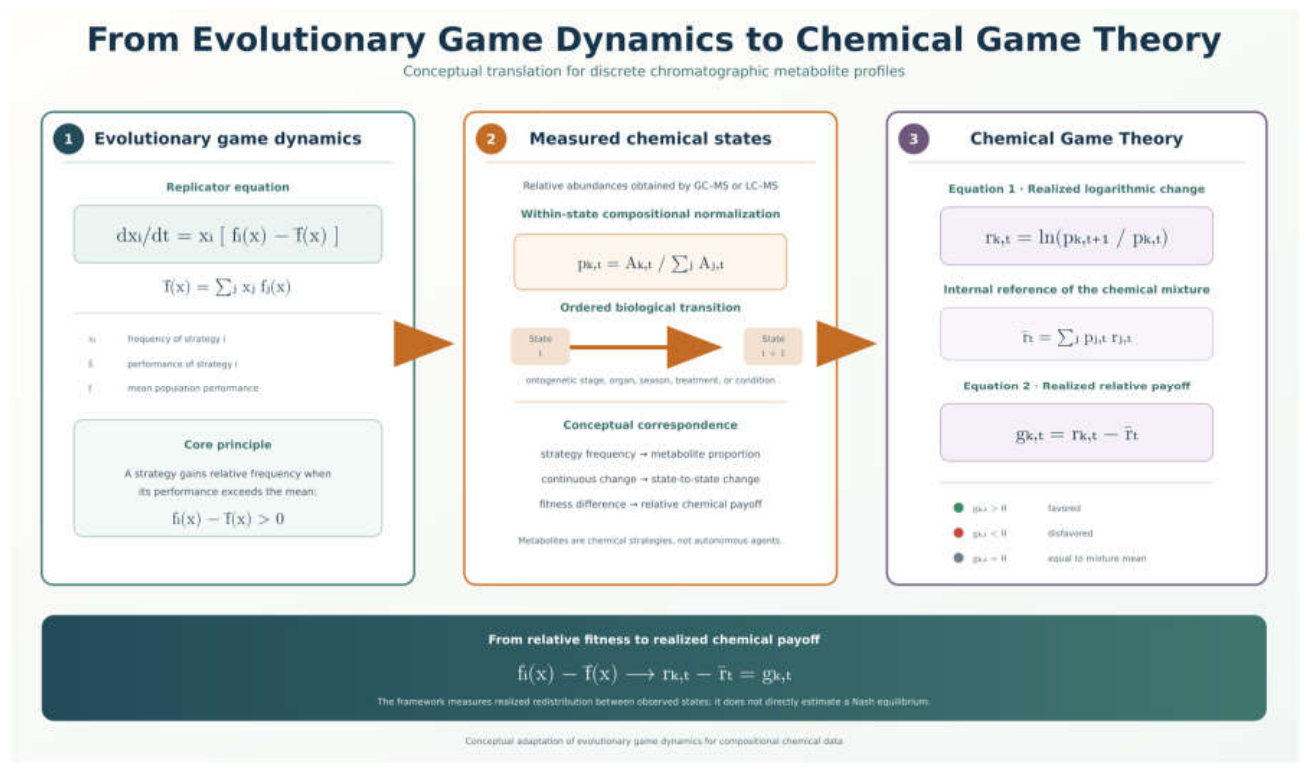
Figure 1. Conceptual translation from evolutionary game dynamics to Chemical Game Theory. The replicator equation describes changes in strategy frequency according to the difference between individual and mean population performance. In Chemical Game Theory, chromatographic relative abundance, p k , t , represents the proportional participation of metabolite k in chemical state t . Continuous evolutionary change is translated into the realized logarithmic change, r k , t , between consecutive biological states. The abundance-weighted mean change of the mixture, r t , provides the internal reference against which the realized relative payoff, g k , t , is calculated. Positive and negative payoffs indicate chemical strategies that gained or lost proportional representation relative to the overall reorganization of the mixture, respectively. Metabolites are treated as chemical strategies within a compositional system, not as autonomous biological agents. The framework quantifies realized redistribution between measured states and does not directly estimate a Nash equilibrium.
Preprints 227202 g001
Figure 2. Conceptual framework of Chemical Game Theory applied to plant chemodiversity. Chromatographic constituents are represented as elementary chemical strategies, whereas biosynthetic pathways constitute higher-order strategies. Shannon diversity describes metabolite coexistence, the General Biosynthetic Diversity Index, GBDI, characterizes biosynthetic architecture, and replicator-based realized payoffs quantify the directional advantage or disadvantage of each strategy between consecutive chemical states. The framework can be applied to ontogenetic, temporal, spatial, environmental, and experimental trajectories. Potential applications include chemical ecology, evolutionary interpretation, conservation, and rational bioprospection.
Preprints 227202 g002
Figure 3. Compound-level Shannon diversity (A) and GBDI (B) across leaves and four reproductive stages of Piper mollicomum. Columns represent monthly sampling blocks. Higher Shannon values indicate greater metabolite richness and evenness, whereas GBDI additionally incorporates the distribution of metabolites within biosynthetic pathways [2,3,4,5,8]. Leaves were used as a vegetative reference and were not included in the ordered reproductive payoff trajectory.
Preprints 227202 g003
Figure 4. Mean biosynthetic-pathway allocation in leaves and reproductive stages of Piper mollicomum. Bars represent normalized pathway abundance averaged across five monthly blocks. The contrast between leaves and reproductive organs demonstrates that high compound-level diversity may occur within one strongly dominant biosynthetic pathway. Sep = September; Oct = October; Nov =November; Dec = December; Jan = January.
Preprints 227202 g004
Figure 5. Joint trajectories of Shannon diversity and GBDI during reproductive-organ development. Lines connect Stages I–IV within each monthly block. Leaf profiles are shown as independent vegetative reference points. Differences among trajectories indicate that ontogenetic chemical reorganization was influenced by the monthly context. Sep = September; Oct = October; Nov =November; Dec = December; Jan = January.
Preprints 227202 g005
Figure 7. Abundance-weighted realized payoff impacts of selected metabolites during reproductive development. Positive values identify metabolites contributing to relative chemical expansion, and negative values identify compounds contributing to contraction. The figure distinguishes high-payoff rare components from quantitatively influential metabolites.
Preprints 227202 g007
Figure 8. General analytical workflow for applying Chemical Game Theory to chromatographic chemodiversity data. GC–MS or LC–MS peak identity and abundance data are curated, harmonized, classified by chemical class and biosynthetic pathway, and normalized by compositional closure. Conventional chemical-state descriptors, including Shannon diversity, Pielou evenness, pathway entropy, dominance, and GBDI, are calculated before ordering samples along a biologically meaningful trajectory. Transition-specific log growth is centered relative to the abundance-weighted chemical background to obtain realized chemical payoff. Payoff sign, payoff impact, positive-payoff frequency, and zero-replacement sensitivity are subsequently integrated to identify relative chemical expansion, contraction, and candidate ontogenetic windows for target prioritization.
Preprints 227202 g008
Table 1. Chemodiversity, biosynthetic architecture, and chemical dominance in leaves and reproductive stages of Piper mollicomum.
Compartment or stage Shannon H′ GBDI Pielou
J
Pathway
entropy Hpath
Dominant-metabolite
abundance pmax
Dominant-pathway
abundance Pmax
Leaves 2.751 ± 0.322 1.735 ± 0.108 0.748 0.125 0.280 0.977
Stage I 1.787 ± 0.408 1.175 ± 0.195 0.701 0.626 0.388 0.668
Stage II 1.963 ± 0.640 1.265 ± 0.283 0.764 0.499 0.318 0.802
Stage III 2.214 ± 0.435 1.414 ± 0.163 0.671 0.554 0.356 0.763
Stage IV 1.925 ± 0.421 1.324 ± 0.156 0.668 0.425 0.407 0.848
Friedman p 0.1933 0.0299 0.0755 0.0018 0.2052 0.0018
Table 2. Mean relative allocation among the principal biosynthetic pathways in leaves and reproductive stages of Piper mollicomum.
Compartment or stage Terpenoid pathway (%) Mixed pathway (%) Shikimate pathway (%) Other pathways (%)
Leaves 97.68 ± 1.37 0.52 ± 0.86 1.03 ± 0.76 0.77
Stage I 66.83 ± 9.31 33.07 ± 9.20 0.05 ± 0.11 0.05
Stage II 80.15 ± 7.81 19.40 ± 7.98 0.38 ± 0.60 0.07
Stage III 76.32 ± 10.54 23.00 ± 9.57 0.46 ± 0.72 0.22
Stage IV 84.78 ± 4.50 15.14 ± 4.46 0.08 ± 0.12 <0.01
Table 3. Realized payoffs of the principal biosynthetic pathways during reproductive development.
Transition Biosynthetic pathway Mean realized payoff g Positive monthly blocks Mean payoff impact Chemical interpretation
Stage I→Stage II Terpenoid 0.269 ± 0.191 5/5 0.196 Consistent relative expansion
Stage I→Stage II Mixed −0.518 ± 0.418 0/5 −0.126 Consistent relative contraction
Stage I→Stage II Shikimate 0.837 ± 0.824 5/5 0.0037 High relative gain but low quantitative influence
Stage II→Stage III Terpenoid −0.002 ± 0.146 3/5 0.0018 Approximately neutral
Stage II→Stage III Mixed 0.246 ± 0.802 2/5 0.0517 Strong temporal dependence
Stage II→Stage III Shikimate 0.076 ± 0.696 4/5 0.0014 Small and variable component
Stage III→Stage IV Terpenoid 0.153 ± 0.176 5/5 0.116 Consistent relative expansion
Stage III→Stage IV Mixed −0.340 ± 0.204 0/5 −0.071 Consistent relative contraction
Stage III→Stage IV Shikimate −0.594 ± 1.431 3/5 −0.0053 Low-abundance, unstable response
Table 4. Relationship between Realized payoff, impact and proposed chemical interpretation.
Realized payoff Abundance or Impact Chemical Interpretation
High High Major expanding chemical strategy
High Low Emerging or rare chemical strategy
Negative High Major contracting chemical strategy
Negative Low Minor or declining chemical strategy
Table 5. Distribution and candidate ontogenetic windows of selected constituents.
Compound Leaves (%) Stage I (%) Stage II (%) Stage III (%) Stage IV (%) Highest observed state
Linalool 14.19 10.12 19.54 20.59 28.34 Stage IV, September, 56.58%
1,8-Cineole 15.64 14.74 15.03 12.57 17.43 Stage IV, December, 37.43%
Eupatoriochromene 0.52 33.07 19.40 23.00 15.14 Stage I, November, 47.86%
α-Pinene 9.54 1.75 4.46 2.41 3.72 Leaves
β-Pinene 8.37 3.63 3.75 4.06 5.61 Leaves
Limonene 1.51 11.65 9.41 4.39 2.59 Stage I, September, 41.83%
Camphor 1.34 0.41 0.02 2.41 2.61 Stage IV, October, 12.70%
E-Caryophyllene 1.51 3.02 3.28 2.93 2.53 Stage II, December, 7.30%
Disclaimer/Publisher’s Note: The statements, opinions and data contained in all publications are solely those of the individual author(s) and contributor(s) and not of MDPI and/or the editor(s). MDPI and/or the editor(s) disclaim responsibility for any injury to people or property resulting from any ideas, methods, instructions or products referred to in the content.
Copyright: This open access article is published under a Creative Commons CC BY 4.0 license, which permit the free download, distribution, and reuse, provided that the author and preprint are cited in any reuse.