
Submitted:
05 August 2026
Posted:
06 August 2026
You are already at the latest version
Abstract
Counter-diabatic Shortcut to Adiabaticity (CDSTA) has been explored in implementing qudit quantum Fourier transforms (QFT) via stimulated Raman adiabatic passage (STIRAP) to suppress non-adiabatic leakage. While direct CD driving may introduce unwanted global microwave couplings, seeking an approach without explicit CD fields is highly desirable. By employing rotating-frame absorption, we implement an all-optical STA strategy to synthesize the QFT. Our systematic comparison of qubit and quartit encodings across Average Gate Fidelity, peak amplitude, and energy cost elucidates the practical advantages brought by qudit architecture and CD driving, demonstrating an acceleration factor of at least 7. Furthermore, we extend our evaluation to open quantum systems. Based on the trade-off analysis, optimized parameters are selected, revealing that the all-optical strategy maintains significant advantages against amplitude noise, pure dephasing, and spontaneous emission, improving robustness against infidelity by an order of magnitude.
Keywords:
counter-diabatic driving
; quantum householder reflection
; quantum fourier transform
; STIRAP
; open system
1. Introduction
The quantum Fourier transform (QFT) forms the basis of quantum algorithms [1], including phase estimation [2], order finding, Shor’s algorithm [3,4], and quantum simulation [5,6]. It is typically implemented via the quantum circuit, utilizing a sequence of Hadamard gates, controlled-phase gates, and SWAPs. For a system of n qubits, this standard approach dictates a circuit complexity of , resulting in prolonged gate execution times.
Two perspectives are used in order to accelerate the operation time. The first focuses on compressing circuit depth, such as improved decompositions [7,8], approximate circuits [9] and hardware-native compilation [10], or high-dimensional (qudit) encoding [11,12,13,14,15,16]. Qudit encodings are being developed both in quantum error correction [17,18] and in quantum communication [19] and being proven to have advantages in specific contexts. Moreover, qudit is often a distinct regime of the same physical carrier rather than a distinct device [20], which indicates that expanding from qubit to qudit is a natural direction. Such a strategy reduces the number of subsystems necessary to represent quantum information and is naturally comparable between different encodings via stimulated Raman adiabatic passage (STIRAP) [21,22], which enables robust adiabatic transfer. The computational states of a single atom may be read either as a quartit or as qubits, which makes the comparison of the two encodings on identical hardware a well-posed question. The explicit mapping uses quantum Householder reflection (QHR), which encodes the quantum information into the Stokes and pumps in STIRAP [23,24,25].
The other method focuses on accelerating physical realization itself, among which the counter-diabatic shortcut to adiabaticity (CDSTA) eliminates the non-adiabatic effect at the Hamiltonian level through inverse engineering [26,27,28,29,30]. Combining CDSTA with STIRAP yields stimulated Raman shortcut-to-adiabatic passage (STIRSAP) [31,32,33,34], which has been demonstrated across various quantum platforms such as cold atoms [35,36,37,38,39,40,41,42,43]. Recently, Ref. [44] realized arbitrary QHR operators via a two-step STIRSAP sequence and applied them to synthesize the quartit QFT, using explicit shortcut pulses.
STIRSAP contains the coupling between ground states, which may involve microwave coupling [27], which generally manifests as a global field and cannot be focused onto a single atom in isolation [45,46,47]. At the same time, CD terms in STIRSAP can be eliminated in a rotating frame [48,49] and absorbed into the modulation of Stokes and pumps [50,51]. Based on this concept, exploring all-optical STIRSAP without explicit CD couplings is meaningful.
In this work, we build on this QHR-STIRSAP route and extend it in three directions. First, instead of explicit shortcut pulses, we use an all-optical STIRSAP that absorbs the CD term into the pump and Stokes fields, removing the ground-state microwave coupling; we address the boundary conditions this requires, left open in Ref. [49], with a super-Gaussian window. Second, we introduce the two-qubit decomposition as a benchmark and perform a three-objective trade-off analysis (fidelity, integrated energy, peak amplitude). Third, we extend the evaluation to open quantum systems under amplitude noise, pure dephasing, and spontaneous emission, using Average Gate Fidelity, in a form that accounts for leakage out of the computational subspace, rather than a single-input state fidelity to remove initial-state bias. We analyze conventional STIRAP, direct STIRSAP, and all-optical STIRSAP throughout.
2. Hamiltonian for QHR-Based QFT
Within a d-dimensional Hilbert space, the QFT is defined by [1,52]
which maps computational basis state to an equal-weight superposition. For an n-qubit register (), conventional circuit architectures dictate a scaling depth of .
Concurrently, the d-dimensional QFT functions as the natural qudit generalization of the Hadamard gate. The unitary operations indispensable for both aforementioned circuit architectures can be synthesized through quantum Householder reflections (QHRs) [23], which are defined as
where denotes a normalized state vector alongside an arbitrary phase shift . Any d-dimensional unitary gate admits a decomposition into at most d sequential QHRs, yielding the product sequence .
To realize the QHR, we employ a -level system (Figure 1) comprising an ancillary ground state and an excited state . Within the rotating-wave approximation, the interaction Hamiltonian for the STIRAP process written in the basis of is given by
where denotes the zero matrix; throughout this work, bold symbols denote column vectors. The pump components share a common temporal envelope and are proportional to the components of the encoded state ,
where is the scalar pump envelope, which also defines the mixing angle .
States orthogonal to remain decoupled, thereby reducing the full -level dynamics to an effective three-level system spanned by [24]. A decoupled dark state, , governs the system evolution. Sweeping from 0 to and back drives the population from the computational basis into the ancillary state and subsequently returns it. By inscribing the required phase during this return trajectory, a complete QHR is synthesized via two consecutive STIRAP sequences. Unfortunately, executing this full population transfer demands a substantial pulse area, inherently bottlenecking the ultimate gate speed.
3. Counter-Diabatic Acceleration and Its All-Optical Implementation
While non-adiabatic leakage fundamentally limits the operational speed of STIRAP, counter-diabatic shortcuts to adiabaticity (CDSTAs) mitigate such errors via the introduction of an auxiliary Hamiltonian [27,31,32],
where denotes the instantaneous eigenstates of . This auxiliary Hamiltonian is designed to cancel the off-diagonal non-adiabatic coupling terms in the adiabatic frame, thereby suppressing transitions between the instantaneous eigenstates and enforcing adiabatic following. Back in the full -dimensional Hilbert space spanned by , this auxiliary drive manifests as a direct coupling between the states and :
where with the scalar amplitude and [38]
Within our framework, the transition constitutes a ground-state-to-ground-state coupling, typically demanding microwave-frequency drives. In atomic arrays, however, such microwave fields can induce spatial crosstalk, thereby violating the strict requirement for site-selective, localized interactions dictated by QFT. To circumvent this limitation, the CD driving can be absorbed into the amplitude and phase modulations of the native Stokes and pump pulses via a unitary transformation [48,49], a framework designated as all-optical STIRSAP. The transformed Hamiltonian is given by
while the modified optical fields are recast as
Note that the formula here differs from that in Ref. [49] due to the different convention used for . Through this approach, the required microwave-frequency coupling is eliminated while the engineered optical pulses retain the original efficacy of CD driving to suppress non-adiabatic transitions.
4. Application to : Quartit vs. Two-Qubit QFT
4.1. STIRAP and STIRSAP Implementation
Our comparative analysis centers on the QFT, defined by
contrasting the implementation performance across qubit and quartit architectures.
Under the conventional qubit mapping, the circuit admits a factorization into Hadamard, controlled-S, and SWAP gates (Figure 2), cumulatively demanding six discrete QHRs. Spanned by the multi-qubit computational basis , the constituent operations are parameterized as and , where the corresponding vectors are given by and . Furthermore, each single-qubit Hadamard operation necessitates two QHRs with a phase shift of . For instance, the tensor product acts on a four-dimensional space that can be decoupled into two independent two-dimensional subspaces: one spanned by and the other spanned by . To synthesize this operation, we construct two state vectors:
The reflection is supported on the subspace , acting as the identity operation on the remaining basis states. Conversely, is supported on . Since the vectors are orthogonal, their corresponding reflections commute. The product of these two reflections transforms each two-dimensional block, yielding . An analogous orthogonal decomposition holds for . The numerical simulations for the two-qubit QFT synthesis are implemented using these constructed vectors.
The native quartit QFT directly coincides with the quartit Hadamard gate, structured as
where and . This alternative paradigm collapses the implementation complexity to a mere two QHR pulses. The quartit encoding reduces the integrated pulse energy by a factor of 3 relative to the two-qubit decomposition, independent of T, reflecting the 4-versus-12 STIRAP-sequence count.
We employ Gaussian pulse profiles parameterized as
with set to the state vector of the k-th QHR. Here we set the peak Rabi frequency to a dimensionless value of . The pulse separation is configured as , and the total integration interval of , thereby scaling all temporal dynamics by the dimensionless pulse width T. This delay is chosen to keep the modulated all-optical waveforms well-conditioned near the pulse edges. Because the peak Rabi frequency is held fixed, varying T does not merely rescale the time axis: the pulse area scales as and the integrated energy as . Throughout, the integrated energy is quantified by
summed over all STIRAP sequences, each integrated over its own duration. All Rabi frequencies are in units of and time in the corresponding dimensionless units, so E carries no prefactor. The CD term vanishes for STIRAP, is counted only for STIRSAP, and for the all-optical scheme is contained in the modulated fields. Since every QHR uses a normalized pump vector, each sequence costs , giving ; at this yields 782 and 261 for the two-qubit and quartit decompositions. Thus, T simultaneously parameterizes the gate duration, the pulse area, and the energy cost, and it is T that controls the degree of adiabaticity.
To enforce the boundary conditions and within finite simulation limits, we introduce a super-Gaussian window function
with hyperparameters and . This mathematical windowing forces the pulse profiles to satisfy the boundary conditions at both temporal extremities.
The numerical scan over the pulse width is shown in Figure 3a to Figure 3d, and each STIRAP is divided into 1000 time steps in . Our findings indicate that the gate fidelity within the non-adiabatic regime exhibits a pronounced sensitivity to the choice of initial states and the STIRSAP protocol eliminates this state-dependent variance.
To dissect this phenomenon, we focus on the quartit STIRAP sequence evaluated at in Figure 4a and Figure 4b. In this regime, non-adiabatic leakage inherently degrades the coupled bright-state branch , leaving its orthogonal complement unperturbed. The initial QHR of this operation targets the state vector . Consider an arbitrary input configuration parameterized by , where the independent angle governs the initial amplitude distribution (, ). Projecting this generic state onto yields the fractional population . Assuming that leakage transitions invariably scatter the population out of the computational manifold, the non-adiabatic attenuation and concomitant phase shift distorting the coupled branch can be encapsulated by a complex error factor . Consequently, the operational fidelity collapses to a deterministic quadratic function of x [53],
To average out the state-dependent deviations discussed above, we evaluate the system performance using the Average Gate Fidelity (AGF) [54,55]. Since the dynamics unfolds in the full -dimensional space, population transferred into and is not guaranteed to return to the computational manifold, so the map obtained by projecting the evolved computational basis states back onto is not unitary. The standard expression for the AGF presumes a unitary U and therefore implicitly attributes the leaked population back to the gate. We instead employ its generalization to non-unitary maps [56],
here and . Eq. (20) reduces to the familiar unitary form whenever , i.e. in the leakage-free limit; retaining ensures that population lost from the computational subspace is correctly counted as infidelity. We set the AGF threshold as 0.99 in Figure 5 and scan . In order to avoid a single point being higher than 0.99, we consider the threshold reached when the five data points after a data point are all higher than 0.99. Without a power constraint, both qubit and quartit STIRAP protocols meet the threshold at under this fixed pulse configuration, while STIRSAP meets it across the entire scanned range down to . CD driving thus removes the adiabatic time floor of STIRAP; the associated peak-power cost is analyzed in Section 5.1.
Here, the decrease in fidelity stems primarily from the non-adiabatic leakage term:
where the represents the root-mean-square (rms) Rabi frequency and the corresponding exponent represents the pulse area, which introduces a dynamical phase during the evolution. By neutralizing non-adiabatic couplings, the STIRSAP suppresses transient excitations to the bright state across the entire evolution. As a direct physical consequence, the operational fidelity becomes decoupled from the accumulated dynamical phase, thereby lifting the stringent constraints previously imposed on the pulse area and enabling high fidelity in small T.
4.2. All-Optical STIRSAP via Rotating-Frame Absorption
CD drivings in STIRSAP act as ground-state couplings, which can be an obstacle in local operations. By transforming the system to a rotating frame with operator , CD drivings are absorbed into Stokes and pumps, as is shown in Eqs. (9)–(). Since second-order derivatives are involved here, the choice of boundary conditions requires greater care to fulfill
Our super-Gaussian window still satisfies the boundary conditions. The resulting temporal waveforms for the first quartit all-optical STIRSAP pulses are delineated in Figure 6 as a demonstration of the modulated waveform.
The AGF of both STIRSAP and all-optical STIRSAP arrives above 0.9999, and Figure 7 shows the difference in AGF between them, exhibiting a ratio that is bounded below and mostly at . This validates that the all-optical STIRSAP replicates the acceleration capabilities of STIRSAP.
The choice of encoding affects circuit depth but does not accelerate the QFT; the acceleration is contributed by CD driving. The encoding still matters once energy and power are considered, as shown next.
5. Discussion
5.1. Comparison
The all-optical protocol suppresses non-adiabatic leakage by reproducing the counter-diabatic coupling through modulated optical fields rather than an explicit microwave drive, thereby canceling the non-adiabatic transitions in the adiabatic frame. Absorbing the CD term into the pump raises the peak amplitude and integrated energy relative to direct STIRSAP; the magnitude of this optical overhead, however, depends strongly on the pulse width T, which motivates the trade-off analysis below.
We employ a three-dimensional Pareto-frontier analysis to simultaneously minimize the maximum instantaneous Rabi frequency , minimize the integrated energy cost (parameterized by ), and minimize the Average Gate Infidelity (AGI=1-AGF). Formulating this as a standard minimization problem, we define the configuration vector as follows:
A configuration dominates if and only if it is less than or equal across all components, and less in at least one:
While direct STIRSAP achieves higher fidelity with lower energy in the idealized closed-system simulation, it requires global microwave driving. Because experimental feasibility is platform-dependent and cannot be easily quantified, we exclude direct STIRSAP from this hardware–cost trade-off analysis.
By scanning the pulse width T from 0.5 to 30, we extract all non-dominated solutions to construct the optimal frontier (Figure 8).
The optical overhead of the all-optical protocol is strongly T-dependent, as shown in Figure 9. For , its peak amplitude exceeds that of direct STIRSAP by less than (e.g., versus at ), with an integrated-energy increase of about at the same T. This overhead arises from absorbing the CD term into the pump; it is bounded, decreases monotonically with T (Figure 9), and does not accumulate with gate count or system size, so it is not amplified in larger circuits. At smaller T, the second-order derivative entering diverges near the pulse edges and the peak amplitude grows rapidly, which is why the all-optical solutions enter the frontier only for . In this regime, the all-optical scheme trades this fixed overhead for the complete removal of the microwave coupling, which is required for site-selective QFT in atomic arrays and cannot be obtained within the direct-STIRSAP framework by spending more energy.
CD driving removes the adiabatic time floor: direct STIRSAP keeps the AGF near unity down to arbitrarily small T while STIRAP requires , so direct STIRSAP sets the acceleration upper bound. This bound is a theoretical limit, since the peak Rabi frequency diverges as . The all-optical scheme is its microwave-free realization: for , it reproduces the CD acceleration and matches the fidelity of direct STIRSAP at the same T (Table 1), at the bounded energy overhead discussed above, while removing the microwave coupling.
Table 1 compares the six protocols. STIRAP is reported at its threshold , and the CD-based protocols at , the smallest width where the all-optical peak overhead remains below . At the same T, the all-optical strategy matches the fidelity of direct STIRSAP at the bounded energy overhead noted above. The factor-of-3 energy reduction is contributed by the quartit encoding, not by the all-optical scheme: it holds across all three protocols and follows exactly from the 4-versus-12 STIRAP-sequence count, since each QHR uses a normalized pump vector and therefore costs the same integrated energy per sequence.
5.2. Noise Resilience in Open Quantum Systems
The noise resilience examined here originates from the CD-accelerated trajectory rather than from the all-optical implementation specifically: by shortening the excited-state exposure, CD driving improves robustness relative to STIRAP. Direct STIRSAP shares this CD trajectory and is therefore expected to perform comparably to the all-optical scheme under noise; we accordingly compare the all-optical protocol against STIRAP, for which the difference is most pronounced. Based on the Pareto analysis, we evaluate whether this advantage holds under realistic noise [57]. At small T, standard STIRAP is dominated by non-adiabatic errors, precluding an open-system comparison. We therefore select , where both protocols lie on the Pareto frontier and maintain an AGF exceeding .
Amplitude noise, originating from laser intensity drifts, is modeled as a static scaling for [58,59]. Pure dephasing is simulated via the Lindblad master equation:
with dephasing rate and the linear-shift jump operator . The AGI was calculated by the density matrix generated by the Monte Carlo method for .
Pure dephasing gives a trajectory-independent error floor, while amplitude noise () induces unitary control errors via dynamic phase mismatch, allowing us to probe both channels.
As is shown in Figure 10, the transition of the contour lines from curved to horizontal marks the threshold where the AGI from amplitude noise is dominated by pure dephasing. When the contour lines become horizontal, it indicates that the system is dominated by pure dephasing and has reached the theoretical limit. In this scenario, the protocol saturates the fidelity upper bound dictated by the environment, rendering the system robust against coherent pulse imperfections [29].
For the standard STIRAP protocol [Figure 10(b)], this transition to dephasing dominance occurs around . The all-optical STIRSAP protocol [Figure 10(a)] exhibits horizontal contours earlier, for , while maintaining a broader high-fidelity plateau in the low-dephasing regime. This earlier decoupling from amplitude noise confirms that the all-optical waveforms rectify the underlying unitary errors. By suppressing the parameter-sensitive unitary defects, the all-optical protocol drives the operational performance closer to the noise limit.
To model spontaneous emission, we assume that the excited state decays with total rate equally into the five ground states (the ancillary state and the four computational states) [60]. The corresponding Lindblad operators are
where denotes the ground-state manifold, which enters the master equation (25). Physically, the fidelity degradation is proportional to the time-averaged population of the leaky state ; the larger the integrated excited-state occupancy, the stronger the impact of spontaneous emission.
Figure 11 visualizes the fidelity decay induced by spontaneous emission for both frontier configurations at . The all-optical STIRSAP protocol maintains an error suppression roughly an order of magnitude stronger than that of standard STIRAP. This robustness is a direct consequence of the CD-accelerated trajectory, which restricts non-adiabatic leakage and minimizes the integrated temporal exposure to excited-state decay channels.
6. Conclusion
In this work, we proposed an all-optical STIRSAP protocol for QFT synthesis that avoids direct microwave counter-diabatic driving. The system is controlled by a single dimensionless characteristic time T.
Our results separate two levers: CD driving removes the adiabatic time floor of STIRAP, and the quartit encoding lowers the integrated energy by a factor of 3. Together, they make the quartit protocol dominate the qubit encoding in the Pareto analysis over AGI, peak amplitude, and energy cost. Direct STIRSAP sets the theoretical acceleration upper bound; how closely a microwave-free implementation can approach it through parameter optimization or optimal control remains an open question.
The all-optical scheme eliminates the ground-state microwave coupling while matching the fidelity of direct STIRSAP, demonstrating its feasibility for quantum algorithms. Its value is thus separable into three contributions: the factor-of-3 energy reduction from the quartit encoding, the noise resilience from CD driving (shared with direct STIRSAP and shown here against STIRAP), and the removal of microwave coupling, which is unique to the all-optical realization. Relative to STIRAP, the suppressed excited-state population further improves robustness against spontaneous emission.
Future work could compare our work with parameter optimization methods or optimal control to deepen the understanding of the underlying dynamics.
Funding
This research received no external funding.
Data Availability Statement
The original contributions presented in the study are included in the article. The numerical simulation code used to generate the results in this work is available on Zenodo at https://doi.org/10.5281/zenodo.21757938.
Acknowledgments
During the preparation of this manuscript, the author used Google Gemini 3.1 Pro and Anthropic Claude Opus 4.8 for the purpose of English language polishing and improving the readability of the text. The author has reviewed and edited all output, confirms that it faithfully reflects the author’s own scientific views and conclusions.
Conflicts of Interest
The authors declare no conflicts of interest.
References
- Nielsen, M.A.; Chuang, I.L. Quantum computation and quantum information; Cambridge University Press: Cambridge, UK, 2010. [Google Scholar] [CrossRef]
- Kitaev, A.Y. Quantum measurements and the Abelian stabilizer problem. arXiv 1995. [Google Scholar]
- Shor, P.W. Algorithms for quantum computation: discrete logarithms and factoring. In Proceedings of the Proceedings 35th Annual Symposium on Foundations of Computer Science; IEEE, 1994; pp. 124–134. [Google Scholar] [CrossRef]
- Shor, P.W. Polynomial-time algorithms for prime factorization and discrete logarithms on a quantum computer. SIAM Rev. 1999, 41, 303–332. [Google Scholar] [CrossRef]
- Vartiainen, J.J.; Niskanen, A.O.; Nakahara, M.; Salomaa, M.M. Implementing Shor’s algorithm on Josephson charge qubits. Phys. Rev. A 2004, 70, 012319. [Google Scholar] [CrossRef]
- Ruiz-Perez, L.; Garcia-Escartin, J.C. Quantum arithmetic with the quantum Fourier transform. Quantum Inf. Process. 2017, 16, 152. [Google Scholar] [CrossRef]
- Hales, L.; Hallgren, S. An improved quantum Fourier transform algorithm and applications. In Proceedings of the Proceedings 41st Annual Symposium on Foundations of Computer Science; IEEE, 2000; pp. 515–525. [Google Scholar] [CrossRef]
- Floratos, E.; Pavlidis, A. A Novel Finite Fractional Fourier Transform and its Quantum Circuit Implementation on Qudits. arXiv 2024. [Google Scholar]
- Choi, J.; Kim, J. A tutorial on quantum approximate optimization algorithm (QAOA): Fundamentals and applications. In Proceedings of the 2019 international conference on information and communication technology convergence (ICTC); IEEE, 2019; pp. 138–142. [Google Scholar] [CrossRef]
- Bäumer, E.; Tripathi, V.; Seif, A.; Lidar, D.; Wang, D.S. Quantum Fourier transform using dynamic circuits. Phys. Rev. Lett. 2024, 133, 150602. [Google Scholar] [CrossRef] [PubMed]
- Deller, Y.; et al. Quantum approximate optimization algorithm for qudit systems. Phys. Rev. A 2023, 107, 062410. [Google Scholar] [CrossRef]
- Kiktenko, E.O.; et al. Single qudit realization of the Deutsch algorithm using superconducting many-level quantum circuits. Phys. Lett. A 2015, 379, 1409–1413. [Google Scholar] [CrossRef]
- Castro, A.; et al. Optimal control of molecular spin qudits. Phys. Rev. Appl. 2022, 17, 064028. [Google Scholar] [CrossRef]
- Wang, Y.; et al. Qudits and high-dimensional quantum computing. Front. Phys. 2020, 8, 589504. [Google Scholar] [CrossRef]
- Bottarelli, A.; de Andoin, M.G.; Chandarana, P.; Paul, K.; Chen, X.; Sanz, M.; Hauke, P. Symmetry-enhanced counterdiabatic quantum algorithm for qudits. Phys. Rev. Res. 2025, 7, 043030. [Google Scholar] [CrossRef]
- Tancara, D.; Albarrán-Arriagada, F. High dimensional counterdiabatic quantum computing. npj Quantum Inf. 2025, 11, 116. [Google Scholar] [CrossRef]
- Brock, B.L.; Singh, S.; Eickbusch, A.; Sivak, V.V.; Ding, A.Z.; Frunzio, L.; Girvin, S.M.; Devoret, M.H. Quantum error correction of qudits beyond break-even. Nature 2025, 641, 612–618. [Google Scholar] [CrossRef] [PubMed]
- Ma, Y.; Hanks, M.; Kim, M. Non–pauli errors can be efficiently sampled in qudit surface codes. Phys. Rev. Lett. 2023, 131, 200602. [Google Scholar] [CrossRef] [PubMed]
- Schmidt, F.; Miller, D.; van Loock, P. Error-corrected quantum repeaters with Gottesman-Kitaev-Preskill qudits. Phys. Rev. A 2024, 109, 042427. [Google Scholar] [CrossRef]
- Maroulakos, D.; Wal, A.; Ugulava, A.; Kharshiladze, O.; Chotorlishvili, L. Quantum skyrmion qudit in a triangular-lattice magnet. Eur. Phys. J. B 2026, 99, 21. [Google Scholar] [CrossRef]
- Vitanov, N.V.; Rangelov, A.A.; Shore, B.W.; Bergmann, K. Stimulated Raman adiabatic passage in physics, chemistry, and beyond. Rev. Mod. Phys. 2017, 89, 015006. [Google Scholar] [CrossRef]
- Unanyan, R.; Fleischhauer, M.; Shore, B.W.; Bergmann, K. Robust creation and phase-sensitive probing of superposition states via stimulated Raman adiabatic passage (STIRAP) with degenerate dark states. Opt. Commun. 1998, 155, 144–154. [Google Scholar] [CrossRef]
- Ivanov, P.A.; Kyoseva, E.S.; Vitanov, N.V. Engineering of arbitrary U(N) transformations by quantum Householder reflections. Phys. Rev. A 2006, 74, 022323. [Google Scholar] [CrossRef]
- Rousseaux, B.; Guérin, S.; Vitanov, N.V. Arbitrary qudit gates by adiabatic passage. Phys. Rev. A 2013, 87, 032328. [Google Scholar] [CrossRef]
- Rezai, M.; Salehi, J.A. Fundamentals of quantum Fourier optics. IEEE Trans. Quantum Eng. 2022, 4, 1–22. [Google Scholar] [CrossRef]
- Torrontegui, E.; et al. Shortcuts to adiabaticity. In Advances in Atomic, Molecular, and Optical Physics; Elsevier: Amsterdam, The Netherlands, 2013; Vol. 62, pp. 117–169. [Google Scholar] [CrossRef]
- Guéry-Odelin, D.; et al. Shortcuts to adiabaticity: Concepts, methods, and applications. Rev. Mod. Phys. 2019, 91, 045001. [Google Scholar] [CrossRef]
- Duncan, C.W.; et al. Taming quantum systems: a tutorial for using shortcuts-to-adiabaticity, quantum optimal control, and reinforcement learning. PRX Quantum 2025, 6, 040201. [Google Scholar] [CrossRef]
- Stefanatos, D.; Paspalakis, E. Optimal shortcuts of stimulated Raman adiabatic passage in the presence of dissipation. Philos. Trans. R. Soc. A 2022, 380, 20210283. [Google Scholar] [CrossRef] [PubMed]
- Singhal, U.; et al. Robust gates inspired by stimulated Raman adiabatic passage for a superconducting dual-rail qubit. Phys. Rev. Appl. 2025, 23, 014044. [Google Scholar] [CrossRef]
- Berry, M.V. Transitionless quantum driving. J. Phys. A Math. Theor. 2009, 42, 365303. [Google Scholar] [CrossRef]
- Demirplak, M.; Rice, S.A. Adiabatic population transfer with control fields. J. Phys. Chem. A 2003, 107, 9937–9945. [Google Scholar] [CrossRef]
- Demirplak, M.; Rice, S.A. Assisted adiabatic passage revisited. J. Phys. Chem. B 2005, 109, 6838–6844. [Google Scholar] [CrossRef] [PubMed]
- Demirplak, M.; Rice, S.A. On the consistency, extremal, and global properties of counterdiabatic fields. J. Chem. Phys. 2008, 129, 154105. [Google Scholar] [CrossRef] [PubMed]
- Hu, C.K.; et al. Experimental implementation of generalized transitionless quantum driving. Opt. Lett. 2018, 43, 3136–3139. [Google Scholar] [CrossRef] [PubMed]
- Black, K.; et al. Shortcut to adiabaticity improvement of STIRAP based qubit rotation. J. Phys. A Math. Theor. 2025, 58, 415304. [Google Scholar] [CrossRef]
- Flament, E.; et al. Unitary transformations using robust optimal control on a cold atom qudit. Phys. Rev. Res. 2025, 7, 033069. [Google Scholar] [CrossRef]
- Chen, X.; et al. Shortcut to adiabatic passage in two-and three-level atoms. Phys. Rev. Lett. 2010, 105, 123003. [Google Scholar] [CrossRef] [PubMed]
- Ruschhaupt, A.; Chen, X.; Alonso, D.; Muga, J.G. Optimally robust shortcuts to population inversion in two-level quantum systems. New J. Phys. 2012, 14, 093040. [Google Scholar] [CrossRef]
- Chen, X.; Muga, J.G. Engineering of fast population transfer in three-level systems. Phys. Rev. A 2012, 86, 033405. [Google Scholar] [CrossRef]
- Corgier, R.; et al. Fast manipulation of Bose–Einstein condensates with an atom chip. New J. Phys. 2018, 20, 055002. [Google Scholar] [CrossRef]
- Masuda, S.; Nakamura, K.; del Campo, A. High-fidelity rapid ground-state loading of an ultracold gas into an optical lattice. Phys. Rev. Lett. 2014, 113, 063003. [Google Scholar] [CrossRef] [PubMed]
- Chen, Y.H.; et al. Shortcuts to adiabaticity for the quantum Rabi model: Efficient generation of giant entangled cat states via parametric amplification. Phys. Rev. Lett. 2021, 126, 023602. [Google Scholar] [CrossRef] [PubMed]
- Ebrahimpour, M.; Saadati-Niari, M.; Shirkhanghah, N. Creation of quantum Householder reflection using shortcut to adiabatic passage. J. Mod. Opt. 2026, 73, 190–200. [Google Scholar] [CrossRef]
- Du, Y.X.; et al. Experimental realization of stimulated Raman shortcut-to-adiabatic passage with cold atoms. Nat. Commun. 2016, 7, 12479. [Google Scholar] [CrossRef] [PubMed]
- Wu, X.; Liang, X.; Tian, Y.; Yang, F.; Chen, C.; Liu, Y.C.; Tey, M.K.; You, L. A concise review of Rydberg atom based quantum computation and quantum simulation. Chin. Phys. B 2021, 30, 020305. [Google Scholar] [CrossRef]
- Stefanatos, D.; Blekos, K.; Paspalakis, E. Robustness of STIRAP shortcuts under Ornstein-Uhlenbeck noise in the energy levels. Appl. Sci. 2020, 10, 1580. [Google Scholar] [CrossRef]
- Ibáñez, S.; et al. Multiple Schrödinger pictures and dynamics in shortcuts to adiabaticity. Phys. Rev. Lett. 2012, 109, 100403. [Google Scholar] [CrossRef] [PubMed]
- Li, Y.C.; Chen, X. Shortcut to adiabatic population transfer in quantum three-level systems: Effective two-level problems and feasible counterdiabatic driving. Phys. Rev. A 2016, 94, 063411. [Google Scholar] [CrossRef]
- Jian, X.X.; et al. All-optical Raman control of ultracold atomic hyperfine states using the pulsed jump protocol. Phys. Rev. A 2025, 112, 013108. [Google Scholar] [CrossRef]
- Ali, A.; et al. Counterdiabatic Raman atom optics for compact high-sensitivity gravimetry. arXiv 2026. [Google Scholar] [CrossRef]
- Cao, Y.; Peng, S.G.; Zheng, C.; Long, G.L. Quantum Fourier transform and phase estimation in qudit system. Commun. Theor. Phys. 2011, 55, 790–794. [Google Scholar] [CrossRef]
- Shore, B.W. Manipulating quantum structures using laser pulses; Cambridge University Press: Cambridge, UK, 2011. [Google Scholar] [CrossRef]
- Nielsen, M.A. A simple formula for the average gate fidelity of a quantum dynamical operation. Phys. Lett. A 2002, 303, 249–252. [Google Scholar] [CrossRef]
- Janković, D.; et al. Noisy qudit vs multiple qubits: conditions on gate efficiency for enhancing fidelity. npj Quantum Inf. 2024, 10, 59. [Google Scholar] [CrossRef]
- Pedersen, L.H.; Møller, N.M.; Mølmer, K. Fidelity of quantum operations. Phys. Lett. A 2007, 367, 47–51. [Google Scholar] [CrossRef]
- Ali, A.; et al. Bright-state source cancellation in dissipative shortcut Raman atom optics. arXiv 2026. [Google Scholar] [CrossRef]
- Laforgue, X.; Dridi, G.; Guérin, S. Optimal robust stimulated Raman exact passage by inverse optimization. Phys. Rev. A 2022, 105, 032807. [Google Scholar] [CrossRef]
- Xu, T.N.; Liu, K.; Chen, X.; Guerin, S. Invariant-based optimal composite stimulated Raman exact passage. J. Phys. B At. Mol. Opt. Phys. 2019, 52, 235501. [Google Scholar] [CrossRef]
- Liu, K.; Sugny, D.; Chen, X.; Guérin, S. Optimal pulse design for dissipative-stimulated Raman exact passage. Entropy 2023, 25, 790. [Google Scholar] [CrossRef] [PubMed]
Figure 1.
Schematic realization of QHR in a -level system. The generalized reflection is implemented via a double-STIRAP sequence mapping the encoded state to the auxiliary state and back.
Figure 1.
Schematic realization of QHR in a -level system. The generalized reflection is implemented via a double-STIRAP sequence mapping the encoded state to the auxiliary state and back.
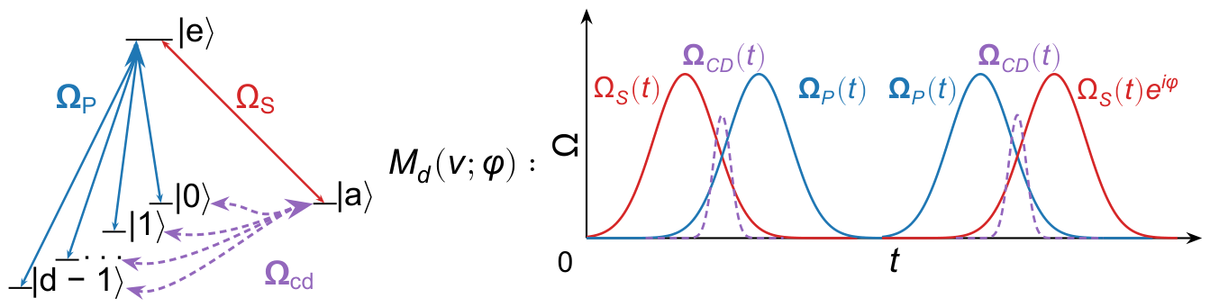
Figure 2.
The two-qubit quantum circuit that realizes the QFT. Hadamard, controlled-S, and SWAP gates are required. These quantum gates serve as the target unitaries for the QHR synthesis.
Figure 2.
The two-qubit quantum circuit that realizes the QFT. Hadamard, controlled-S, and SWAP gates are required. These quantum gates serve as the target unitaries for the QHR synthesis.
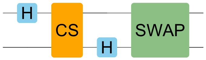
Figure 3.
Initial-state sensitivity of the four protocols. Initial states are generated through the Monte Carlo method. State fidelity is defined as . We scan the dimensionless pulse duration T from 0.1 to 20. Shaded regions depict the minimum-to-maximum fidelity and lines represent the mean fidelity, both after exponential fitting. (a) The two-qubit STIRAP (red dotted line); (b) qubit STIRSAP (orange dashed line); (c) quartit STIRAP (blue dash-dotted line); and (d) quartit STIRSAP (green solid line). This comparison indicates that initial state sensitivity originates from the non-adiabatic effect and can be suppressed by CDSTA.
Figure 3.
Initial-state sensitivity of the four protocols. Initial states are generated through the Monte Carlo method. State fidelity is defined as . We scan the dimensionless pulse duration T from 0.1 to 20. Shaded regions depict the minimum-to-maximum fidelity and lines represent the mean fidelity, both after exponential fitting. (a) The two-qubit STIRAP (red dotted line); (b) qubit STIRSAP (orange dashed line); (c) quartit STIRAP (blue dash-dotted line); and (d) quartit STIRSAP (green solid line). This comparison indicates that initial state sensitivity originates from the non-adiabatic effect and can be suppressed by CDSTA.
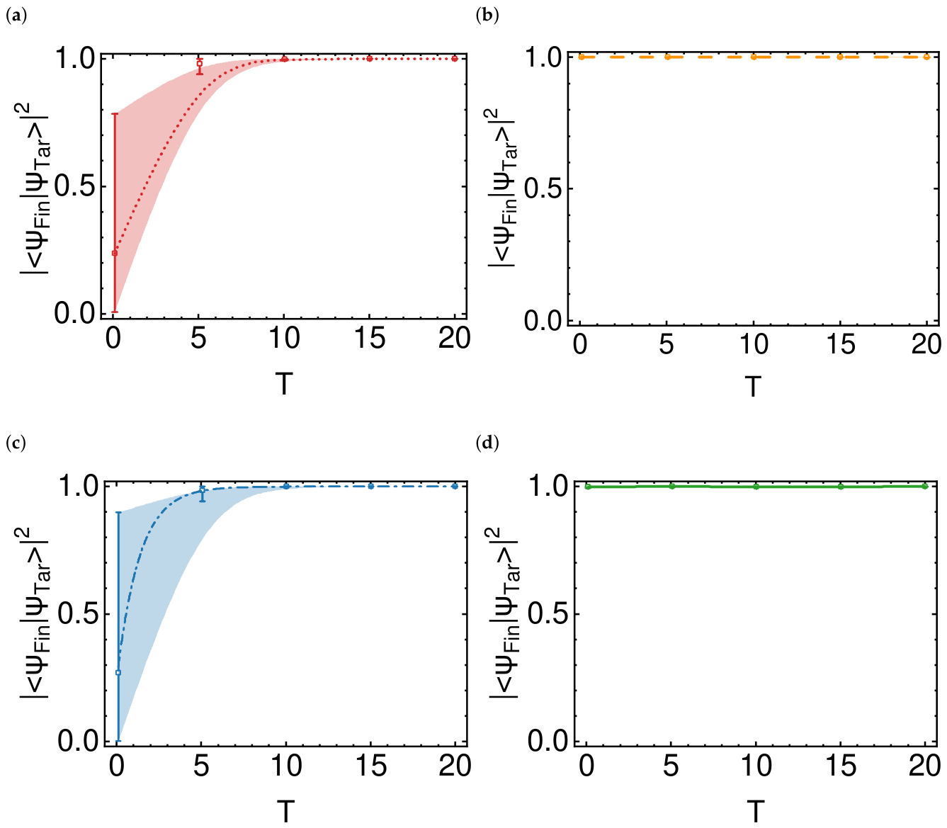
Figure 4.
Initial-state dependence of quartit STIRAP in the non-adiabatic regime (). (a) Heatmap of the operational fidelity scanned over the initial state parameters and the relative phase . This global scan illustrates the sensitivity of the fidelity to the initial state composition when the adiabatic condition is violated. (b) State fidelity at with a minimum at . This occurs when the initial state aligns with the target bright state and maximizes the population leakage.
Figure 4.
Initial-state dependence of quartit STIRAP in the non-adiabatic regime (). (a) Heatmap of the operational fidelity scanned over the initial state parameters and the relative phase . This global scan illustrates the sensitivity of the fidelity to the initial state composition when the adiabatic condition is violated. (b) State fidelity at with a minimum at . This occurs when the initial state aligns with the target bright state and maximizes the population leakage.
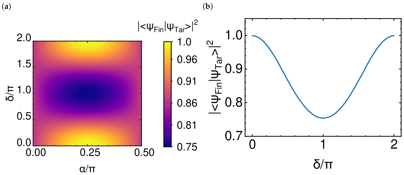
Figure 5.
Average Gate Fidelity (AGF) as a function of pulse width plotted on a logarithmic scale. Each STIRAP/STIRSAP is discretized into 1000 time steps in . Continuous curves are generated via B-spline interpolation of the simulated data points. A protocol is designated to reach when five consecutive data points surpass this threshold. Both the qubit STIRAP decomposition (red dotted line) and the quartit STIRAP (blue dash-dotted line) meet the threshold at . By contrast, both the qubit STIRSAP (orange dashed line) and quartit STIRSAP (green solid line) meet it at , illustrating the speed-up afforded by CDSTA.
Figure 5.
Average Gate Fidelity (AGF) as a function of pulse width plotted on a logarithmic scale. Each STIRAP/STIRSAP is discretized into 1000 time steps in . Continuous curves are generated via B-spline interpolation of the simulated data points. A protocol is designated to reach when five consecutive data points surpass this threshold. Both the qubit STIRAP decomposition (red dotted line) and the quartit STIRAP (blue dash-dotted line) meet the threshold at . By contrast, both the qubit STIRSAP (orange dashed line) and quartit STIRSAP (green solid line) meet it at , illustrating the speed-up afforded by CDSTA.
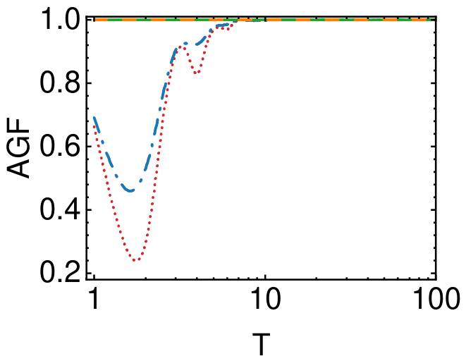
Figure 6.
Modulated Stokes (red solid line) and pumps (blue dashed and green dotted lines) for the first quartit all-optical STIRSAP at , plotted against the normalized time . Guided by explicit CD terms, the optical pulse waveforms are optimized, achieving a shortcut to adiabaticity.
Figure 6.
Modulated Stokes (red solid line) and pumps (blue dashed and green dotted lines) for the first quartit all-optical STIRSAP at , plotted against the normalized time . Guided by explicit CD terms, the optical pulse waveforms are optimized, achieving a shortcut to adiabaticity.
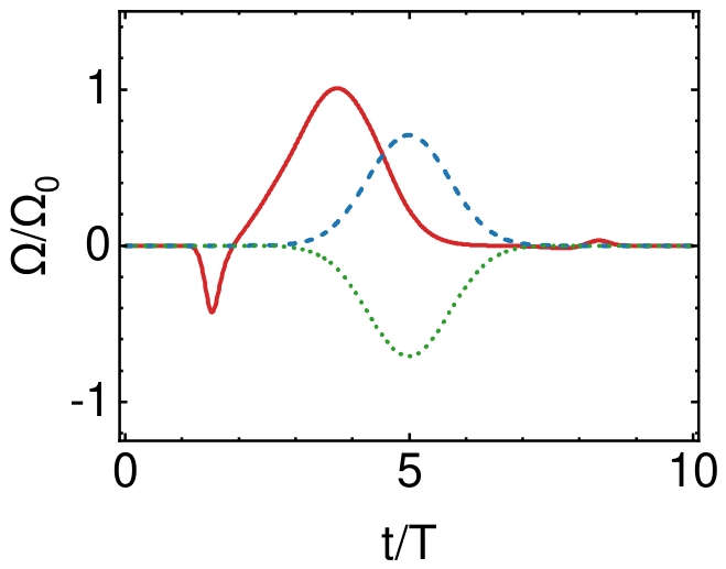
Figure 7.
Statistical verification of the equivalence between the direct and all-optical STIRSAP protocols of the qubit (blue dotted line) and quartit (green solid line) architectures. The histograms display the absolute percentage deviation between them and the lines represent fits to the respective count distributions. Most data points lie within , and the maximum deviation is under . This demonstrates the equivalence between STIRSAP and all-optical STIRSAP.
Figure 7.
Statistical verification of the equivalence between the direct and all-optical STIRSAP protocols of the qubit (blue dotted line) and quartit (green solid line) architectures. The histograms display the absolute percentage deviation between them and the lines represent fits to the respective count distributions. Most data points lie within , and the maximum deviation is under . This demonstrates the equivalence between STIRSAP and all-optical STIRSAP.
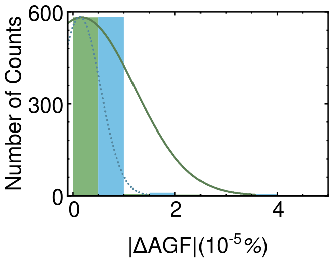
Figure 8.
Pareto-frontier analysis across Average Gate Infidelity (), integrated energy cost (), and maximum Rabi frequency (, color map), shown as the projection. Filled markers are the three-objective Pareto-optimal points (STIRAP, squares; STIRSAP, circles; all-optical, triangles); grey open diamonds are dominated points, with transparency separating qubit and quartit points. All qubit points are dominated, so the frontier consists only of quartit configurations. Inset: Working-region zoom where each STIRSAP (circle) and all-optical (triangle) pair at equal T nearly coincides, with the triangle lying slightly at higher energy.
Figure 8.
Pareto-frontier analysis across Average Gate Infidelity (), integrated energy cost (), and maximum Rabi frequency (, color map), shown as the projection. Filled markers are the three-objective Pareto-optimal points (STIRAP, squares; STIRSAP, circles; all-optical, triangles); grey open diamonds are dominated points, with transparency separating qubit and quartit points. All qubit points are dominated, so the frontier consists only of quartit configurations. Inset: Working-region zoom where each STIRSAP (circle) and all-optical (triangle) pair at equal T nearly coincides, with the triangle lying slightly at higher energy.
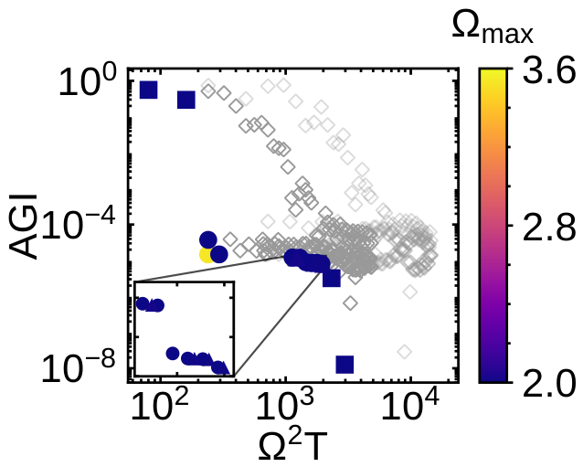
Figure 9.
Relative excess of the all-optical peak amplitude over direct STIRSAP as a function of T. The curve is identical for the qubit and quartit encodings, since it depends only on the ratio . The excess drops below for and diverges at small T due to the second-order derivative in .
Figure 9.
Relative excess of the all-optical peak amplitude over direct STIRSAP as a function of T. The curve is identical for the qubit and quartit encodings, since it depends only on the ratio . The excess drops below for and diverges at small T due to the second-order derivative in .
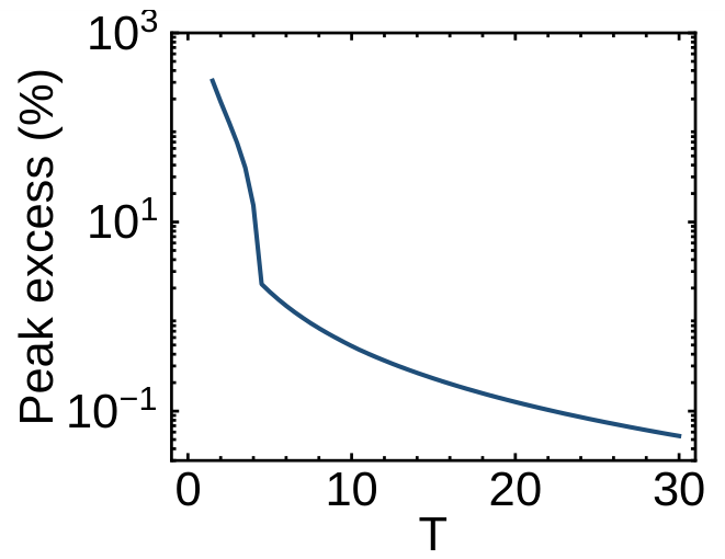
Figure 10.
Noise resilience analysis of the two protocols under pure dephasing and amplitude noise. (a) All-optical STIRSAP, where the contour lines become horizontal (dephasing-dominated) for . In the amplitude-noise-dominated regime (), it maintains a broader high-fidelity plateau, demonstrating robustness against unitary errors. (b) Quartit STIRAP, where the transition to horizontal contours occurs later, around . The earlier onset of dephasing dominance in the all-optical protocol indicates a suppression of unitary control errors, pushing the system’s performance closer to the fidelity upper bound dictated by the environment.
Figure 10.
Noise resilience analysis of the two protocols under pure dephasing and amplitude noise. (a) All-optical STIRSAP, where the contour lines become horizontal (dephasing-dominated) for . In the amplitude-noise-dominated regime (), it maintains a broader high-fidelity plateau, demonstrating robustness against unitary errors. (b) Quartit STIRAP, where the transition to horizontal contours occurs later, around . The earlier onset of dephasing dominance in the all-optical protocol indicates a suppression of unitary control errors, pushing the system’s performance closer to the fidelity upper bound dictated by the environment.
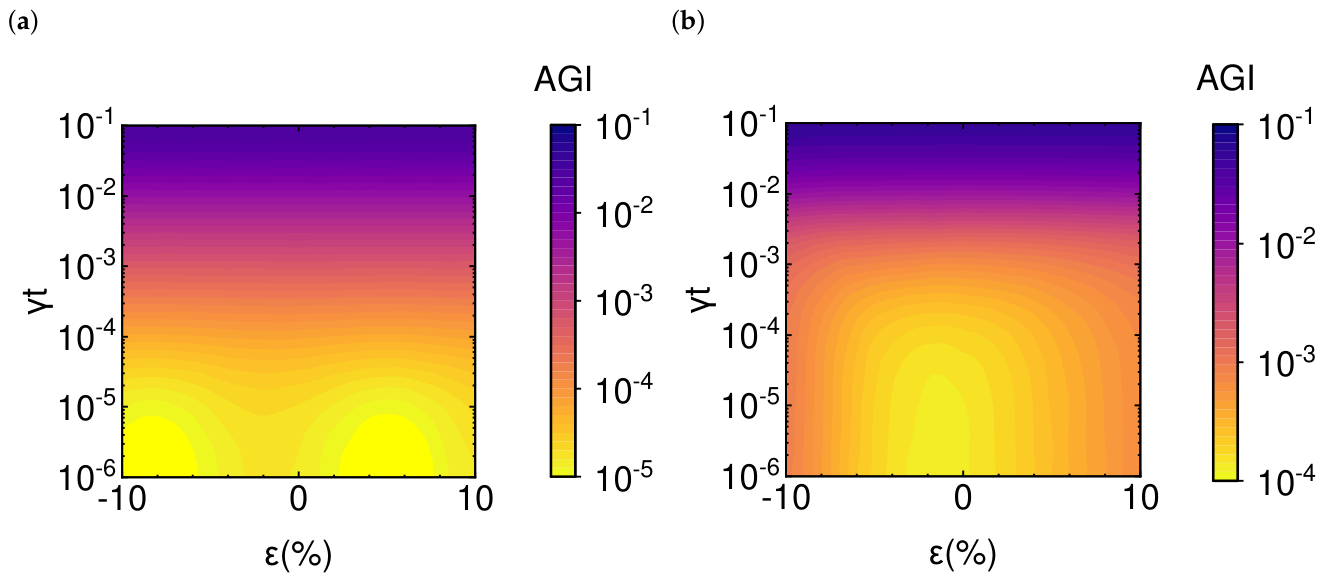
Figure 11.
Effect of spontaneous emission at , quantified by the absolute fidelity deviation as a function of . All-optical STIRSAP exhibits a robustness roughly one order of magnitude higher than that of standard STIRAP, highlighting the reduction in excited-state emission exposure.
Figure 11.
Effect of spontaneous emission at , quantified by the absolute fidelity deviation as a function of . All-optical STIRSAP exhibits a robustness roughly one order of magnitude higher than that of standard STIRAP, highlighting the reduction in excited-state emission exposure.
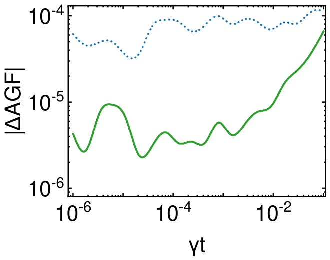

Table 1.
Comparison of the protocols for QFT synthesis. STIRAP is evaluated at its threshold . STIRSAP and the all-optical scheme are shown at ; at the same T, replacing direct STIRSAP by the all-optical scheme adds a bounded overhead (peak , energy ), while the minimal T of direct STIRSAP itself tends to zero. Energy is the integrated cost calculated according to Eq. (17) and is the peak Rabi frequency.
Table 1.
Comparison of the protocols for QFT synthesis. STIRAP is evaluated at its threshold . STIRSAP and the all-optical scheme are shown at ; at the same T, replacing direct STIRSAP by the all-optical scheme adds a bounded overhead (peak , energy ), while the minimal T of direct STIRSAP itself tends to zero. Energy is the integrated cost calculated according to Eq. (17) and is the peak Rabi frequency.
| No. of QHRs | T | AGF | Energy | ||
|---|---|---|---|---|---|
| qubit STIRAP | 6 | 6.5 | 0.99093 | 2.00 | 782 |
| quartit STIRAP | 2 | 6.5 | 0.99499 | 2.00 | 261 |
| qubit STIRSAP | 6 | 4.5 | 0.99995 | 2.00 | 555 |
| quartit STIRSAP | 2 | 4.5 | 0.99997 | 2.00 | 185 |
| qubit all-optical | 6 | 4.5 | 0.99995 | 2.04 | 662 |
| quartit all-optical | 2 | 4.5 | 0.99997 | 2.04 | 221 |
Disclaimer/Publisher’s Note: The statements, opinions and data contained in all publications are solely those of the individual author(s) and contributor(s) and not of MDPI and/or the editor(s). MDPI and/or the editor(s) disclaim responsibility for any injury to people or property resulting from any ideas, methods, instructions or products referred to in the content. |
© 2026 by the authors. Licensee MDPI, Basel, Switzerland. This article is an open access article distributed under the terms and conditions of the Creative Commons Attribution (CC BY) license (http://creativecommons.org/licenses/by/4.0/).
Copyright: This open access article is published under a Creative Commons CC BY 4.0 license, which permit the free download, distribution, and reuse, provided that the author and preprint are cited in any reuse.


