

Submitted:
30 July 2026
Posted:
04 August 2026
You are already at the latest version
Abstract
Finite-distance light-time calculations sometimes subtract physical and reference radial integrals at the same turning radius, even though the two rays then reach different angular endpoints. We formulate the problem for static, spherically symmetric spacetimes and separate this common-turning-point excess from the time-transfer delay between the same source and receiver events. The radial Hamilton--Jacobi characteristic gives \(T=W+b\Phi\) and \(\dd T/\dd\Phi=b\). It follows that endpoint matching is exactly a one dimensional integral in ray space; at first order, δTend=δTr0−brefδΦr0. We derive the corresponding quadratic correction and first-order sensitivity kernels for arbitrary perturbations of the metric functions \(A\), \(B\), and \(C\). Turning-point-regular primitives are then obtained for Schwarzschild, Reissner--Nordstr\"om, and Kottler geometries. Endpoint matching changes the finite Schwarzschild term and halves the far-field coefficient of the leading charge contribution. In Kottler spacetime an exact de~Sitter reference separates background propagation from the static-coordinate lens term; the resulting mixed $M\Lambda$ contribution is a reference-dependent time-transfer building block, not by itself an independent cosmological observable.
Keywords:
Shapiro time delay
; time-transfer function
; optical geometry
; finite-distance lensing
; Hamilton–Jacobi theory
; Kottler spacetime
1. Introduction
In a stationary spacetime, a light-time observable is defined by an emission event, a reception event, and a null-geodesic branch joining them. The coordinate travel time is therefore a time-transfer function of the endpoints, and its derivatives determine the propagation direction and impact parameter [1,2,3]. This endpoint formulation is essential in a lensing configuration, where more than one branch may connect the same events.
Black-hole lensing also provides observables beyond the primary weak-deflection branch. Relativistic images and their differential delays can constrain lens masses and distances, while time-delay and magnification-centroid observables distinguish compact-object geometries [4,5,6]. The strong-field structure is organized geometrically by photon surfaces [7], and complementary image information can be encoded in distortion relations [8]. Plasma and dark-matter environments modify optical propagation [9], whereas eikonal constructions relate unstable null-orbit data to strong lensing, shadows, quasinormal ringing, and grey-body transmission [10]. These developments make it important to distinguish ray-labelled integral differences from delays defined between fixed endpoint events.
Many calculations in black-hole spacetimes instead parameterize a ray by its radial turning point and subtract a reference integral evaluated at the same turning radius. This is a useful intermediate construction, but it is not generally a time-transfer function: the physical and reference angular sweeps differ, so the rays do not share both endpoint events. The distinction is small in a controlled weak-field regime but becomes nonuniform near alignment, where the shift of the reference turning point is enhanced. It is also relevant in nonasymptotically flat geometries, because the reference spacetime and the map between endpoint events must be stated explicitly.
Optical geometry provides a common language for travel time and bending. Null rays in a static spacetime are geodesics of a Riemannian optical metric, and their coordinate travel time is the optical length. The Gauss–Bonnet construction expresses finite-distance deflection through optical curvature and boundary data [11,12,13,14]. In isothermal coordinates the curvature area integral becomes a boundary flux, whereas the first variation of travel time is a line integral of the same conformal perturbation [15,16,17]. These are complementary functionals, but they are not harmonic conjugates.
We develop the endpoint conversion directly from the radial Hamilton–Jacobi characteristic. The exact identity
implies an exact nonlinear matching law in ray space and, at first perturbative order,
Here T is the coordinate travel time, is the continuous azimuthal sweep on a fixed branch, and b is the impact parameter. The label means that the physical and reference quantities are first evaluated at a common turning radius. We also give the quadratic matching term and explicit metric-perturbation kernels that can be applied coefficient by coefficient in a gravitational effective field theory.
Schwarzschild, Reissner–Nordström (RN), and Kottler spacetimes provide closed-form tests. For Schwarzschild we reconcile the areal-coordinate result with the standard first-post-Minkowskian time-transfer function. For Kottler the reference is de Sitter, not Minkowski. This static-patch subtraction must not be confused with an image-to-image cosmological time delay, in which observer motion, angular-diameter distances, and the lens equation reorganize the apparent dependence [18].
We set and use signature . The analysis is restricted to a single-pass weak branch with one simple radial turning point and a reference ray connecting the same endpoint events.
2. Optical Geometry and Complementary Conformal Functionals
2.1. Static Spherical Geometry
Consider
with in the static region. On the equatorial plane, the null condition gives
Thus the coordinate travel time is exactly the optical length,
For conserved and , define . The radial time and azimuthal integrands are
The turning radius satisfies
Unless , is a coordinate turning radius rather than an invariant areal distance.
2.2. Isothermal Coordinates
Introduce an isothermal radius by
Then
In Cartesian coordinates on the conformal plane,
Consequently,
while the travel time is a trace integral of along the ray. The finite-distance deflection additionally contains the geodesic-curvature and corner terms fixed by the closure of the Gauss–Bonnet domain [12,14,16].
For a one-parameter family represented in a common, endpoint-fixing conformal gauge, write . Fermat stationarity then removes the first-order contribution from the displacement of the reference geodesic, and
If the physical and reference isothermal charts are chosen independently, their coordinate identification also moves the endpoint coordinates and the corresponding boundary terms must be retained. The Hamilton–Jacobi construction below instead uses a common chart and is independent of this conformal-gauge choice. Subject to this identification, Equations (12) and (13) show that bending and time transfer probe, respectively, normal-derivative and trace data of the same conformal perturbation. No generic harmonic-conjugate relation follows: black-hole optical curvature is distributed through the vacuum optical manifold, so need not vanish away from the material lens.
3. Endpoint Primitives and Hamilton–Jacobi Matching
3.1. Fixed-Turning-Point Boundary Primitive
For a single-pass ray from S to R through ,
If is an antiderivative of at fixed , then
This is an endpoint representation once the radial integration has been carried out. It does not by itself enforce that a reference ray at the same reaches the same angular endpoints.
Figure 1 illustrates the distinction. The physical ray has turning point P and radius . The endpoint-matched reference ray generally has a different closest approach and radius .
3.2. Radial Characteristic
Define the radial Hamilton–Jacobi characteristic
Because , differentiation of the lower limit gives no contribution. Directly,
Therefore
Differentiating along a fixed pair of endpoint radii yields
This is the relevant conjugacy: travel time is the generating function for the endpoint angular separation. Equivalent derivative relations underlie the time-transfer-function and eikonal approaches of Refs. [1,2].
3.3. From Common to Common Endpoints
Let refer to a perturbed geometry and to a chosen reference geometry, identified in the same chart. At a common , define
The endpoint-matched reference turning radius is determined by
On a branch where is monotonic, Equation (21) gives the exact reference-time shift
Consequently, the exact endpoint conversion is
This form is equivalent to solving Equation (23), but it makes the canonical structure explicit. Expanding the ray-space integral gives
Equation (2) is the first-order truncation.
For equal endpoint radii R in a flat reference, and . Equation (25) then reduces to
which remains useful when the linearized shift of the reference turning point is inaccurate but the same weak reference branch still exists.
3.4. First-order Metric-Perturbation Kernels
The matching formula can be combined with a general perturbation of the static spherical metric. Write
where barred quantities define the reference geometry. At fixed , introduce
The turning-point condition gives and . Varying Equations (6) and (7) yields
Although the last terms contain , they are regular at a simple turning point because . Integrating and on both radial legs gives and , after which Equation (26) performs the endpoint conversion. These kernels apply directly to metric corrections organized by Wilson coefficients; no new geodesic variation is required at first order.
For a Minkowski reference in an areal polar chart, the endpoint-matched kernel takes a particularly simple form. Set
and parameterize each straight reference leg by , with . Fermat stationarity gives directly
Here is the zeroth-order Euclidean closest approach; replacing it by the physical turning radius changes Equation (33) only at second order. This line kernel is equivalent to integrating Equations (30) and (31) and applying the linear term in Equation (26). It supplies a direct route from a static spherical EFT metric to its first-order time-transfer coefficient.
The first-order conversion is local in ray space. It requires the matched reference turning radius to remain perturbatively close to ,
For flat or de Sitter reference rays with , . In a flat reference, For equal distant endpoints in Schwarzschild, Equation (34) reduces parametrically to . The limits and weak endpoint matching are therefore nonuniform near perfect alignment.
The matching is branch dependent. In a lensing configuration there may be several physical rays, and a weak-field reference branch may cease to exist when the continuous angular sweep crosses its limiting value [3]. Near alignment or on multiple-image branches, one should solve Equation (23) without linearization or impose the appropriate lens equation. The closed formulas below apply locally on a single weak, single-pass branch.
4. Example Geometries
For the examples, and . Write
All results retain the exact dependence on at the stated order in M, , and .
4.1. Schwarzschild
For , the turning-point-regular primitive through is
Subtracting the flat primitive at the same gives
The corresponding angular excess is
Since in flat space, Equation (2) yields
Equation (39) agrees with the standard first-post-Minkowskian time-transfer function. To see the coordinate conversion explicitly, let and define the Euclidean endpoint separation
In isotropic Schwarzschild coordinates, . The familiar first-order result is
At fixed angular endpoints,
while
Their sum is Equation (39). The nonlogarithmic term is therefore the radial-coordinate conversion required when the reference endpoints are identified in Schwarzschild areal coordinates, not a disagreement with the usual time-transfer formula [1,2].
In Schwarzschild areal coordinates, the two far-field forms are
The constants are not invariant observables: they depend on the radial coordinate and on the reference matching. Differential arrival times between two rays received by the same observer remove common convention-dependent terms. Equations (42) and (43) are coefficient limits of the finite-distance expressions; the endpoint result must also satisfy Equation (34) and cannot be extrapolated to exact alignment at fixed M.
Figure 2 compares the two definitions for . Both have the same leading logarithm, but the finite matching term separates them. With , the endpoint coefficient obeys
so the quadratic endpoint correction cancels exactly.
4.2. Reissner–Nordstr Öm
For , expand independently in and . The formulas below isolate the coefficient linear in ; terms of order and are not included. At fixed , the charge contribution has integrand and primitive
Thus
The fixed- angular correction is
Endpoint matching therefore gives
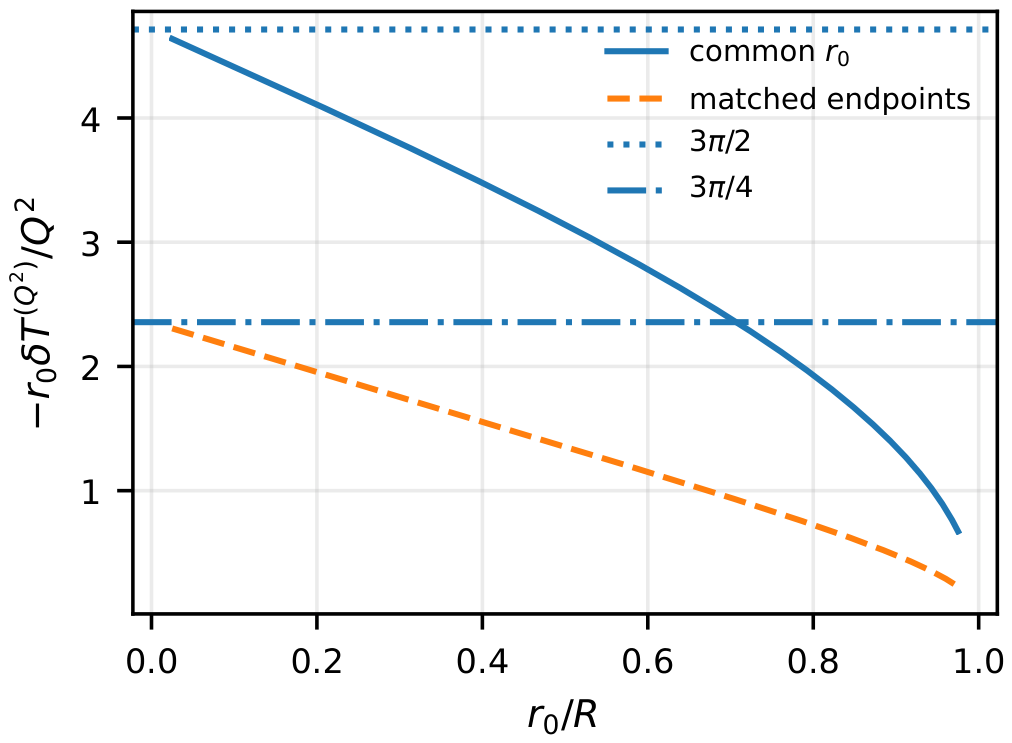
At the displayed order, charge decreases the coordinate light-time coefficient relative to Schwarzschild in both conventions. For ,
The factor-of-two difference is entirely the endpoint-matching term, not a discrepancy in the radial primitive.
Figure 3.
Magnitude of the coefficient linear in for . The ordinate is . The correction vanishes as . The horizontal lines are the far-field limits for common- subtraction and for matched endpoints.
Figure 3.
Magnitude of the coefficient linear in for . The ordinate is . The correction vanishes as . The horizontal lines are the far-field limits for common- subtraction and for matched endpoints.
4.3. Kottler Geometry
For
de Sitter space is the natural background reference in the static patch [19]. Set . The exact de Sitter time primitive is
with . Its small- expansion is
At common , the lens-induced delay relative to de Sitter is
Terms quadratic in M and terms proportional to are omitted. The total common- excess relative to Minkowski additionally contains
which is a background time rather than a lens signal.
The orbit radicand satisfies
so the Kottler angular sweep parametrized by is exactly independent of . The fixed- angular excess relative to de Sitter is therefore Equation (38) at order M. However,
Applying Equation (2) gives
Reference subtraction and endpoint matching are distinct operations. A total delay relative to Minkowski and a lens delay relative to de Sitter must each be defined using endpoint events matched within the corresponding reference problem.
Equation (57) is a static-coordinate time-transfer building block. It does not establish an independent observable effect of in a cosmological lensing delay. In an image-to-image measurement with comoving source and observer, the lens equation, observer motion, proper-time conversion, and angular-diameter distances must be expanded together. An independent analysis of exact Schwarzschild–de Sitter geodesics finds that, at the comparable order considered there, cosmology enters through the unlensed distances and redshift factor rather than an additional local term [18]. The mixed term above instead records how the chosen static de Sitter reference and endpoint identification act before that observable reduction.
Figure 4 uses and remains inside the static patch. The Minkowski subtraction is dominated by the de Sitter background. Subtracting that background exposes the lens coefficient, and endpoint matching adds a finite shift of the same type found in Schwarzschild.
5. Proper Time and Differential Lensing Observables
A static receiver at measures
For two rays a and b received at the same static worldline,
The common lapse factors out, but it does not cancel. It may be set to unity only after normalizing the time coordinate to the receiver or when at the required order.
A measured lensing delay requires each branch to satisfy the same emission event and the appropriate reception condition. Equations (39), (48), and (57) are therefore time-transfer building blocks. Evaluating them at arbitrary values without solving the endpoint condition does not produce an image-to-image observable. Once the branches are fixed, common coordinate- and reference-dependent constants drop from their difference. If the receiver moves, as in a cosmological Kottler setup, the two reception events need not have the same static radius and Equation (59) must be replaced by an integration along the receiver worldline [18].
5.1. Independent Numerical Validation
The primitives and the perturbation kernels were differentiated symbolically. The exact integrals were also evaluated after the change of variable
which removes the square-root turning-point singularity. For the RN–Kottler family,
which is numerically stable near and displays the exact cancellation of from the orbit radicand. A simple turning point requires
which is satisfied throughout the weak-branch tests.
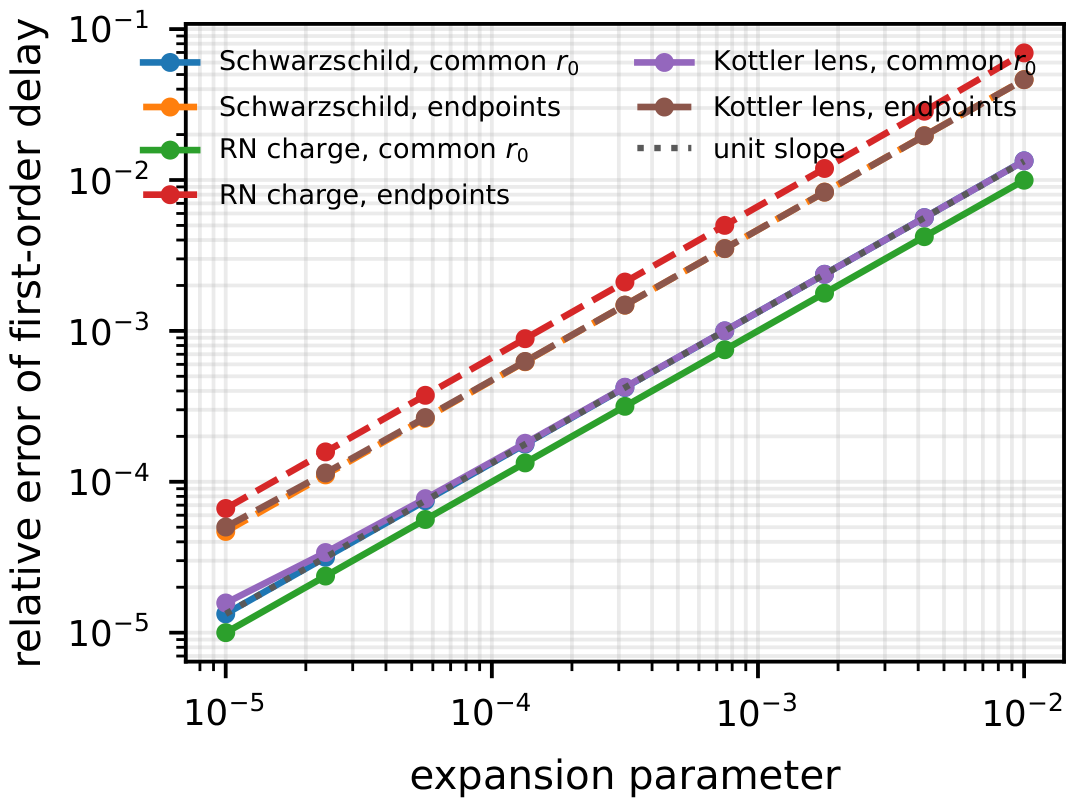
For endpoint-matched tests, the exact physical angular sweep was evaluated first and Equation (23) was then solved for the reference turning radius. Figure 5 uses , expansion parameters from to , and in the Kottler test. The plotted error is . Log–log fits give slopes between and , consistent with an absolute remainder that starts at second order. The upper end of the range also satisfies Equation (34).
6. Discussion
The optical-length identity and the Gauss–Bonnet construction refer to the same two-dimensional optical manifold, but to different data on it. In an endpoint-fixing isothermal chart, the first variation of time samples the conformal perturbation on the reference ray; bending contains its normal derivative together with the boundary closure. Their canonical link is Equation (21), not a harmonic-conjugate relation.
A boundary primitive does not remove the geodesic problem. It performs the radial integration after a branch and turning point have been selected. Equation (25) then supplies the missing endpoint conversion. The distinction matters whenever a common- subtraction is reported as a Shapiro delay: that subtraction compares different angular events unless .
The kernels (30) and (31) separate two effects that are otherwise mixed in a direct expansion: propagation in the perturbed optical metric and displacement of the reference ray needed to keep the endpoints fixed. For a gravitational effective field theory, a, , and c can be expanded in Wilson coefficients and the endpoint conversion applied to each coefficient. A bound on a Wilson coefficient still requires an image or ranging model with the same endpoint convention; an unmatched primitive is not itself an observable.
The present construction assumes a static spherical metric, one simple radial turning point, and no caustic crossing or winding. A static isotropic plasma can be incorporated through its frequency-dependent Riemannian optical metric. Timelike propagation admits a related Jacobi–Maupertuis description [20]. Rotation produces a Randers–Finsler optical geometry; the Hamilton–Jacobi endpoint relation survives, whereas the two-dimensional Riemannian conformal reduction used here does not.
7. Conclusions
Finite-distance time transfer requires both a propagation calculation and an endpoint prescription. A common-turning-radius subtraction provides the first but not, in general, the second. The Hamilton–Jacobi relation converts it to the same-event quantity through the exact ray-space integral (25); Equation (2) and the quadratic term in Equation (26) are its local expansions.
All Schwarzschild, RN, and Kottler primitives pass symbolic derivative checks and exact numerical tests. Endpoint matching changes the finite Schwarzschild contribution and reduces the leading far-field RN charge coefficient from to . In Kottler spacetime, de Sitter subtraction separates background propagation from the static-coordinate lens coefficient, while the final interpretation of any term depends on the complete observable setup. The general perturbation kernels extend the same calculation to static spherical effective metrics without rederiving the endpoint shift for each model.
Data Availability Statement
No external data were used.
Use of Artificial Intelligence
During the preparation of this work the author(s) used ChatGTP in order to improve grammar of paper, and assist with the formatting of LATEX code. After using this tool/service, the author(s) reviewed and edited the content as needed and take(s) full responsibility for the content of the published article. All intellectual content, analysis, and conclusions are the authors’ own.
Acknowledgments
A. Ö. and R. P. would like to acknowledge networking support of the COST Action CA21106 - COSMIC WISPers in the Dark Universe: Theory, astrophysics and experiments (CosmicWISPers), the COST Action CA22113 - Fundamental challenges in theoretical physics (THEORY-CHALLENGES), the COST Action CA21136 - Addressing observational tensions in cosmology with systematics and fundamental physics (CosmoVerse), the COST Action CA23130 - Bridging high and low energies in search of quantum gravity (BridgeQG), and the COST Action CA23115 - Relativistic Quantum Information (RQI) funded by COST (European Cooperation in Science and Technology). R. P. and A. Ö. would also like to acknowledge the funding support of SCOAP3. A. Ö. also thanks to EMU, TUBITAK, ULAKBIM (Turkiye).
Appendix A. Derivative Checks
For Schwarzschild, differentiation of Equation (36) gives
which is the fixed- expansion of Equation (6). The RN derivative follows immediately from
For Kottler,
All perturbative primitives vanish at . The exact de Sitter result also satisfies
which is Equation (6) evaluated in the de Sitter reference metric. For the flat endpoint kernel (33), the Schwarzschild and RN substitutions give, respectively,
Their endpoint evaluations reproduce Equations (39) and (48).
References
- Ashby, N.; Bertotti, B. Accurate light-time correction due to a gravitating mass. Class. Quant. Grav. 2010, 27, 145013, [arXiv:gr-qc/0912.2705]. [CrossRef]
- Linet, B.; Teyssandier, P. New method for determining the light travel time in static, spherically symmetric spacetimes. Calculation of the terms of order G3. Class. Quant. Grav. 2013, 30, 175008, [arXiv:gr-qc/1304.3683]. [Erratum: Class.Quant.Grav. 31, 079502 (2014)], . [CrossRef]
- Linet, B.; Teyssandier, P. Time transfer functions in Schwarzschild-like metrics in the weak-field limit: A unified description of Shapiro and lensing effects. Phys. Rev. D 2016, 93, 044028, [arXiv:gr-qc/1511.04284]. [CrossRef]
- Bozza, V.; Mancini, L. Time delay in black hole gravitational lensing as a distance estimator. Gen. Rel. Grav. 2004, 36, 435–450, [gr-qc/0305007]. [CrossRef]
- Virbhadra, K.S. Relativistic images of Schwarzschild black hole lensing. Phys. Rev. D 2009, 79, 083004, [arXiv:gr-qc/0810.2109]. [CrossRef]
- Virbhadra, K.S.; Keeton, C.R. Time delay and magnification centroid due to gravitational lensing by black holes and naked singularities. Phys. Rev. D 2008, 77, 124014, [arXiv:gr-qc/0710.2333]. [CrossRef]
- Claudel, C.M.; Virbhadra, K.S.; Ellis, G.F.R. The Geometry of photon surfaces. J. Math. Phys. 2001, 42, 818–838, [gr-qc/0005050]. [CrossRef]
- Virbhadra, K.S. Conservation of distortion of gravitationally lensed images. Phys. Rev. D 2024, 109, 124004, [arXiv:gr-qc/2402.17190]. [CrossRef]
- Atamurotov, F.; Abdujabbarov, A.; Han, W.B. Effect of plasma on gravitational lensing by a Schwarzschild black hole immersed in perfect fluid dark matter. Phys. Rev. D 2021, 104, 084015. [CrossRef]
- Lütfüoğlu, B.C.; Rayimbaev, J.; Murodov, S.; Kurbanov, J.; Matyoqubov, M. A First-Order Eikonal Framework for Quasinormal Modes, Shadows, Strong Lensing, and Grey-Body Factors in a Scalarized Black-Hole Metric. Annals Phys. 2026, 491, 170514, [arXiv:gr-qc/2604.14999]. [CrossRef]
- Gibbons, G.W.; Werner, M.C. Applications of the Gauss-Bonnet theorem to gravitational lensing. Class. Quant. Grav. 2008, 25, 235009, [arXiv:gr-qc/0807.0854]. [CrossRef]
- Ishihara, A.; Suzuki, Y.; Ono, T.; Kitamura, T.; Asada, H. Gravitational bending angle of light for finite distance and the Gauss-Bonnet theorem. Phys. Rev. D 2016, 94, 084015, [arXiv:gr-qc/1604.08308]. [CrossRef]
- Ono, T.; Ishihara, A.; Asada, H. Gravitomagnetic bending angle of light with finite-distance corrections in stationary axisymmetric spacetimes. Phys. Rev. D 2017, 96, 104037, [arXiv:gr-qc/1704.05615]. [CrossRef]
- Arakida, H. Light deflection and Gauss–Bonnet theorem: definition of total deflection angle and its applications. Gen. Rel. Grav. 2018, 50, 48, [arXiv:gr-qc/1708.04011]. [CrossRef]
- Pantig, R.C.; Övgün, A. Reference-renormalized curvature-primitive Gauss-Bonnet formalism for finite-distance weak gravitational lensing in static spherical spacetimes. Phys. Rev. D 2026, 113, 104037, [arXiv:gr-qc/2604.16807]. [CrossRef]
- Övgün, A.; Pantig, R.C. Boundary-only weak deflection angles from isothermal optical geometry. Class. Quant. Grav. 2026, 43, 085011, [arXiv:gr-qc/2601.06864]. [CrossRef]
- Pantig, R.C. Endpoint-controlled shadows and the collapse of photon spheres at singular horizons. Phys. Lett. B 2026, 879, 140643. [CrossRef]
- Teodori, L.; Blum, K.; Bai, Z. Gravitational lensing time delay beyond the Shapiro/geometry split 2026. [arXiv:astro-ph.CO/2605.18182].
- Kagramanova, V.; Kunz, J.; Lammerzahl, C. Solar system effects in Schwarzschild-de Sitter spacetime. Phys. Lett. B 2006, 634, 465–470, [gr-qc/0602002]. [CrossRef]
- Jia, J.; Liu, H. Time delay of timelike particles in gravitational lensing of the Schwarzschild spacetime. Phys. Rev. D 2019, 100, 124050, [arXiv:gr-qc/1906.11833]. [CrossRef]
Figure 1.
Finite-distance matching in the conformal plane. The physical optical geodesic connects S and R and turns at P. The dotted reference ray is constrained to have the same and therefore misses R. The dashed reference ray connects the prescribed endpoints and has turning point , with in general. The drawing is schematic; the physical geodesic is not assumed to be a Euclidean conic.
Figure 1.
Finite-distance matching in the conformal plane. The physical optical geodesic connects S and R and turns at P. The dotted reference ray is constrained to have the same and therefore misses R. The dashed reference ray connects the prescribed endpoints and has turning point , with in general. The drawing is schematic; the physical geodesic is not assumed to be a Euclidean conic.
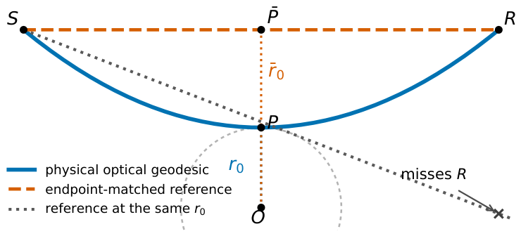
Figure 2.
Schwarzschild first-order coefficient for . The solid and dashed curves show common- and endpoint-matched subtraction, respectively. The dotted and dash-dotted curves are the corresponding far-field expansions. Both finite-distance coefficients vanish as ; the far-field curves do not apply in that limit.
Figure 2.
Schwarzschild first-order coefficient for . The solid and dashed curves show common- and endpoint-matched subtraction, respectively. The dotted and dash-dotted curves are the corresponding far-field expansions. Both finite-distance coefficients vanish as ; the far-field curves do not apply in that limit.
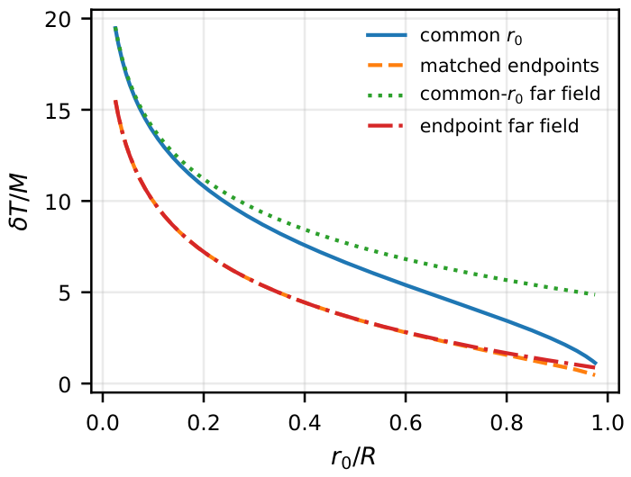
Figure 4.
Kottler decomposition for and . The dotted curve is the exact de Sitter background. The dashed and dash-dotted curves retain the lens terms of order M and at common and matched endpoints, respectively; the solid curve is the sum of the exact background and the common- lens truncation. Here . The value of is chosen to separate the curves visually and is not an astrophysical forecast.
Figure 4.
Kottler decomposition for and . The dotted curve is the exact de Sitter background. The dashed and dash-dotted curves retain the lens terms of order M and at common and matched endpoints, respectively; the solid curve is the sum of the exact background and the common- lens truncation. Here . The value of is chosen to separate the curves visually and is not an astrophysical forecast.
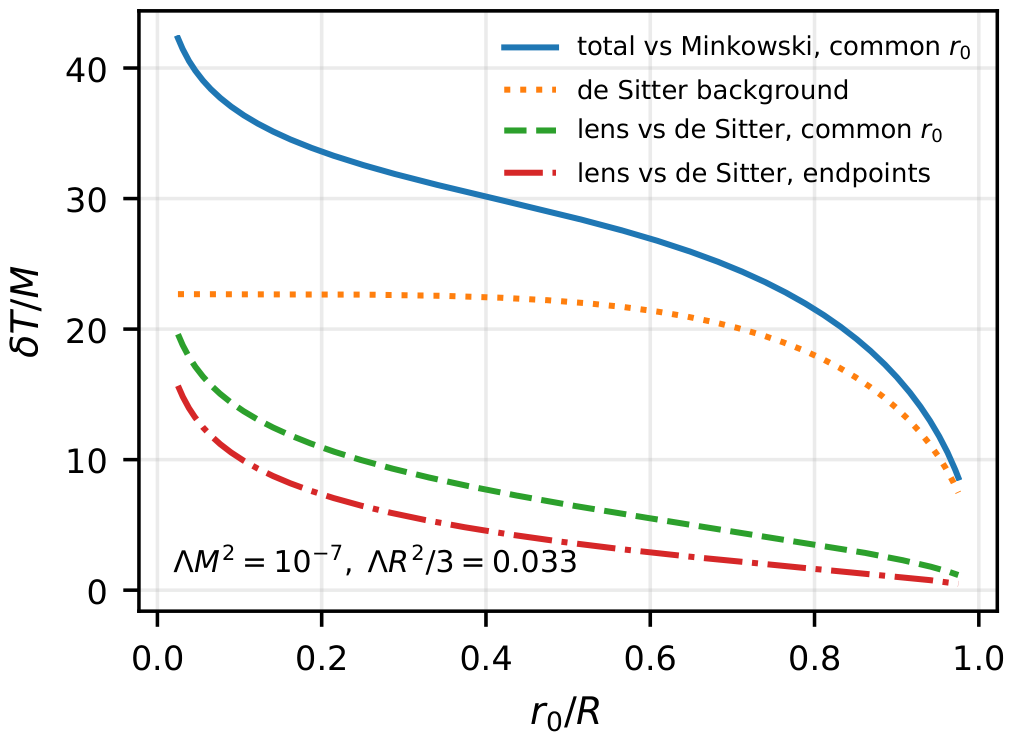
Figure 5.
Relative error of the first-order formulas against exact quadrature for . Solid curves use common- subtraction; dashed curves use exact endpoint matching. The horizontal variable is for Schwarzschild and Kottler and for the RN coefficient. The Kottler curves use . Fitted slopes lie between and .
Figure 5.
Relative error of the first-order formulas against exact quadrature for . Solid curves use common- subtraction; dashed curves use exact endpoint matching. The horizontal variable is for Schwarzschild and Kottler and for the RN coefficient. The Kottler curves use . Fitted slopes lie between and .
Disclaimer/Publisher’s Note: The statements, opinions and data contained in all publications are solely those of the individual author(s) and contributor(s) and not of MDPI and/or the editor(s). MDPI and/or the editor(s) disclaim responsibility for any injury to people or property resulting from any ideas, methods, instructions or products referred to in the content. |
© 2026 by the authors. Licensee MDPI, Basel, Switzerland. This article is an open access article distributed under the terms and conditions of the Creative Commons Attribution (CC BY) license (http://creativecommons.org/licenses/by/4.0/).
Copyright: This open access article is published under a Creative Commons CC BY 4.0 license, which permit the free download, distribution, and reuse, provided that the author and preprint are cited in any reuse.


