

Submitted:
03 August 2026
Posted:
04 August 2026
You are already at the latest version
Abstract
Radiometric interferometry is a powerful technique for angular spacecraft navigation, traditionally implemented through ground-based Very Long Baseline Interferometry (VLBI) and Delta Differential One-Way Ranging. A previously proposed concept, Radiometric Interferometry Navigation using GEO Satellites (RINGS), replaces terrestrial VLBI stations with geostationary satellites in order to create a space-based interferometric baseline for deep-space navigation. The present paper extends the initial RINGS concept by developing a time-position error analysis and by evaluating the impact of practical clock and GEO orbit-determination uncertainties on the reconstructed angle of arrival. The analysis focuses on two main practical error sources: residual relative clock misalignment between the GEO satellites and uncertainty in the GEO station positions that define the interferometric baseline. First, analytical models are developed to map clock timing error and GEO baseline uncertainty into angular error. The clock analysis shows that timing-induced path error is divided by the long GEO-GEO baseline, providing a baseline-leverage advantage relative to terrestrial VLBI. The paper then evaluates GNSS-based synchronization, passive-hydrogen-maser-class clock stability, two-way inter-satellite synchronization and ranging, relativistic and moving-endpoint timing corrections, and GEO orbit-determination uncertainty. A Monte Carlo simulation framework is then used to propagate clock and position perturbations through a dual-frequency RINGS angle-of-arrival estimator. The results show that picosecond to tens-of-picoseconds residual timing errors contribute only small stochastic angular scatter when considered alone. After PHM-class timing and two-way inter-satellite synchronization, a 10ps residual timing level contributes approximately 0.04nrad for a 120∘ three-GEO baseline, while a conservative 100ps residual contributes approximately 0.4nrad. GEO position uncertainty is found to be the dominant error driver once meter-level orbit-determination errors are assumed. Under sub-meter GEO baseline knowledge and picosecond-level inter-satellite synchronization, the simulations support nanoradian-level angular performance. The results strengthen the feasibility case for GEO-based VLBI as a complementary deep-space navigation observable. The main practical requirements identified are accurate relative GEO-GEO baseline knowledge, high-stability onboard timing, two-way inter-satellite synchronization and ranging, deterministic timing-correction modeling, and robust phase-ambiguity resolution.
Keywords:
deep-space navigation
; VLBI
; Delta-DOR
; GEO satellites
; radiometric interferometry
; clock synchronization
; passive hydrogen maser
; inter-satellite time transfer
; orbit determination
; Monte Carlo simulation
1. Introduction
Very Long Baseline Interferometry (VLBI) and Delta Differential One-Way Ranging are established radiometric techniques for deep-space navigation [12]. These methods provide highly accurate angular information by measuring the differential arrival time or phase of a spacecraft radio signal at widely separated receiving stations. In conventional deep-space navigation, the receiving stations are located on Earth, and the achievable angular accuracy depends on baseline length, signal-to-noise ratio, atmospheric calibration, station-location knowledge, clock stability, and observation geometry.
The RINGS concept, Radiometric Interferometry Navigation using GEO Satellites, was introduced as a space-based extension of terrestrial VLBI [11]. Instead of using ground stations as the interferometric receivers, RINGS uses geostationary satellites as the receiving stations. This architecture creates a GEO-to-GEO interferometric baseline of several tens of thousands of kilometers, approaching about for near-antipodal GEO longitude slots. The actual baseline depends on the final orbital slots and longitude separation, based on regulatory and operational constraints. Even when the satellites are not separated by , the resulting baseline remains substantially longer than terrestrial VLBI baselines. The space-based architecture also removes receiver-side tropospheric and ionospheric path errors and improves geometric measurement availability for deep space targets.
The first RINGS study introduced the basic measurement concept and provided a top-down stochastic estimate of the expected angle of arrival (AOA) accuracy. The present paper continues that work by analyzing the two main practical uncertainty mechanisms that dominate a GEO-based implementation: relative clock bias between the GEO receivers and uncertainty in the GEO station positions. These two effects directly affect the interferometric phase observable and therefore the reconstructed angular direction to the spacecraft.
The paper separates analytical modeling from simulation-based validation. The analytical part develops timing requirements, clock stability estimates, two-way inter-satellite synchronization, relativistic timing corrections, and GEO orbit-determination uncertainty ranges. The simulation part then injects these uncertainties into a dual-frequency RINGS AOA estimator and evaluates the resulting angular error through Monte Carlo analysis.
The remainder of this paper is organized as follows. Section 2 develops the analytical error models for clock-error mapping, clock synchronization requirements, passive hydrogen maser stability, two-way inter-satellite time transfer, deterministic timing corrections, and GEO baseline uncertainty. Section 3 presents the simulation methodology and Monte Carlo setup used to propagate clock and GEO position errors through the RINGS angle-of-arrival estimator. Section 4 presents the numerical simulation results, including clock-only sensitivity, GEO position sensitivity, representative AOA reconstruction cases, and combined position-clock performance. Section 5 discusses the dominant error drivers and implications for practical RINGS implementation. Section 6 summarizes the main conclusions and future work.
2. Analytical Error Modeling
This section develops the analytical models used to quantify the two main implementation level uncertainty sources in the RINGS interferometric system: residual clock and timing error between the GEO receivers, and uncertainty in the GEO satellite positions that affects the phase stability and GEO-GEO baseline.
The section first derives the linear relationship between residual relative clock misalignment and angular uncertainty. This derivation also shows the baseline leverage advantage of RINGS: the same timing induced path error is divided by a much longer interferometric baseline than in terrestrial VLBI. The resulting timing requirement is then used to assess GNSS-based synchronization and to motivate the need for a high-stability onboard clock and direct inter satellite synchronization. The following subsections then examine passive hydrogen maser clock stability over the coherent integration window, the two-way inter-satellite time transfer concept, deterministic relativistic and moving-endpoint timing corrections, and finally the GEO orbit determination and baseline error representation used later in the Monte Carlo simulations.
2.1. Clock Error Mapping and Synchronization Requirement
Precise relative timing between the GEO receivers is essential for RINGS. The interferometric observable is based on the relative phase of the spacecraft signal received at two separated GEO stations. A residual synchronization error between the receiver clocks therefore appears as a path-delay error and maps directly into angular error.
A residual timing error corresponds to a path-length uncertainty
where c is the speed of light. The interferometric observable is proportional to the projected GEO-GEO baseline,
where B is the GEO-GEO baseline length and is the angle between the baseline and the line of sight to the spacecraft. Linearizing Eq. (2) gives
A residual clock offset produces the equivalent path-length error
Thus, the clock-induced angular error is linear in the residual clock misalignment. For representative RINGS geometries away from the singular case , the characteristic clock contribution can be written as
Equation (6) is the key clock-sizing relation for RINGS. A clock misalignment produces the same path-delay error regardless of the interferometer architecture, but the resulting angular error is divided by the interferometric baseline. Since the GEO-GEO baseline is much longer than a terrestrial VLBI baseline, the same residual timing error produces a smaller angular perturbation. For two systems with the same timing residual, the relative clock-induced angular error scales as
In nanoradians, Eq. (6) becomes
For a practical three-GEO configuration with approximately separation, the GEO-GEO chord length is
For RINGS, the GEO-GEO baseline depends on the selected orbital slots, satellite longitude separation, and instantaneous GEO geometry. A near-antipodal GEO configuration can approach the maximum GEO chord length,
where . In practice, regulatory approval of GEO slots, line-of-sight constraints, and operational considerations may lead to a shorter baseline. Therefore, the following analysis uses a representative RINGS baseline range of
The timing uncertainty required to support a desired angular uncertainty follows by rearranging Eq. (6):
The first RINGS study estimated terrestrial-VLBI-order angular performance at the few-nanoradian level, with a representative value of approximately [11]. If the full clock contribution were allowed to reach this value, Eq. (12) would give
However, the clock contribution should be only a fraction of the total angular error budget because GEO position uncertainty, receiver noise, calibration residuals, and phase ambiguity also contribute. A more appropriate clock-allocation reference is therefore . For the representative RINGS baseline range, Eq. (12) gives
Equation (14) provides the basic timing boundary: residual relative clock error must be kept below the few-hundred-picosecond level to keep the clock contribution below . In practice, a more conservative synchronization design target is useful in order to preserve margin:
For the representative RINGS baseline range, this corresponds to an angular contribution of approximately
Thus, clock synchronization at the few tens of picoseconds level keeps the clock-induced stochastic angular contribution well below the nanoradian level across the representative RINGS baseline range.
Before considering high-stability onboard clocks, it is useful to examine whether GNSS-based synchronization alone could satisfy this timing requirement. GNSS can provide valuable absolute time anchoring and long-term time reference support, including for spacecraft at GEO altitude when signal availability, receiver sensitivity, and tracking geometry are sufficient [21]. However, GNSS is not sufficient by itself as the primary relative inter-satellite timing observable for RINGS.
Public GPS performance specifications report time-transfer accuracy relative to UTC(USNO), the United States Naval Observatory realization of Coordinated Universal Time, at the tens-of-nanoseconds level [20]. Dedicated GNSS time-transfer methods with high-quality equipment and post-processing can provide improved timing performance under favorable conditions [24]. Therefore, this study uses
as an optimistic representative one-sigma GNSS-based timing uncertainty. This value is not used as a guaranteed GEO performance level, but as a favorable reference case for assessing whether GNSS-based synchronization alone could satisfy the RINGS relative timing requirement.
For two GEO satellites independently synchronized to GNSS time, the relative timing uncertainty is approximately
For the representative RINGS baseline range, this maps into an angular uncertainty of approximately
This value is already within the terrestrial VLBI order of magnitude, but it is too large if the clock contribution is required to remain a small fraction of the total RINGS angular error budget. GNSS-based synchronization can therefore support absolute time anchoring and long-term reference alignment, but it is not sufficient as the primary relative timing observable. A dedicated onboard frequency reference and direct inter-satellite synchronization are required.
The above estimates assume that phase ambiguity is resolved and that the estimator remains on the correct local phase branch. Under that assumption, Eq. (8) provides the direct first-order mapping between residual clock misalignment and RINGS angular uncertainty.
2.2. Clock Stability over the Coherent Integration Window
The short-term stability of an onboard frequency reference is commonly described by the Allan deviation , where is the averaging time [8,9,10]. Allan deviation is a fractional frequency-stability measure. It does not directly represent clock time offset. Rather, it quantifies fractional frequency fluctuations, which accumulate into timing error over a finite observation interval.
For RINGS, the relevant time interval is the coherent VLBI phase-collection window at the two GEO receiving stations. In this study, the representative coherent integration interval is taken as
The desired onboard clock must therefore maintain residual time variation below the required level over the coherent phase-collection interval. Passive hydrogen masers are a natural candidate for this requirement because they combine excellent short-term frequency stability, low long-term frequency drift, and demonstrated space qualification.
Passive hydrogen maser clocks have already been developed, qualified, and flown in European satellite-navigation missions, including Galileo [18]. As a representative onboard clock technology for RINGS, this study considers a space-qualified passive hydrogen maser of the Mini-PHM class. The Mini-PHM is used here as a reference performance level, not as a final payload selection. Representative Allan deviation values reported for the Leonardo space PHM and Mini-PHM class are summarized in Table 1 [19].
The coherent integration window used in the RINGS simulation, , is between the tabulated and values. Assuming white frequency-modulation noise over this interval, the Allan deviation scales approximately as
Therefore, when the averaging time is reduced from to , the Allan deviation increases. This is expected because frequency stability improves with longer averaging time in the white-frequency-noise regime. Using the reference value from Table 1, the corresponding estimate is
This value is also consistent, at order-of-magnitude level, with interpolation between the and Allan deviation values in Table 1.
To estimate the timing impact during the coherent integration window, the fractional frequency stability is converted into an RMS time deviation. For white frequency-modulation noise, an approximate relation is
where represents the short-term stochastic time wander accumulated over the interval . This quantity is different from slowly varying clock offset, frequency bias, clock aging, and calibration residuals.
Substitution of gives
For two independent GEO satellite clocks, the relative timing uncertainty between the two receiving stations is approximately
This value represents the short-term stochastic timing instability over the phase-collection interval. It does not include slowly varying clock offset, residual temperature sensitivity, aging, or calibration residuals. These terms must be estimated and removed through clock calibration, two-way inter-satellite time transfer, and periodic synchronization updates.
Periodic compensation is feasible because Mini-PHM-class passive hydrogen masers exhibit very low long-term frequency drift and temperature sensitivity, with reported values below per day and below , respectively [19]. These characteristics allow slowly varying clock terms to be tracked and calibrated on timescales much longer than the few-minute RINGS phase-collection window.
This result indicates that Mini-PHM-class passive hydrogen maser clocks can support the short-term timing stability required by RINGS over a few-minute coherent integration interval, provided that clock offset, aging, temperature sensitivity, and calibration residuals are handled separately by the synchronization and calibration architecture.
2.3. Two-Way Synchronization and Subsequent Clock Residuals
The clock-stability result in Eq. (25) shows that hydrogen-maser-class clocks can provide approximately relative stochastic timing stability over the coherent integration interval. However, onboard clock stability alone is not sufficient. Slowly varying clock offset, internal hardware delays, and long-term drift must be calibrated. RINGS therefore uses a two-way inter-satellite synchronization concept analogous to classical Two-Way Satellite Time and Frequency Transfer [1,2,3,4]. The method is adapted here to a direct GEO-GEO link.
A two-satellite RINGS geometry with nearly opposite GEO longitudes maximizes baseline length but may not always provide direct inter-satellite line of sight because of Earth blockage. A three-GEO configuration, with satellites separated by approximately , improves inter-satellite connectivity, timing-transfer availability, and baseline diversity. This geometry is shown in Figure 1.
The three-GEO configuration reduces the maximum interferometric baseline moderately relative to the ideal two-satellite separation. However, the added line-of-sight connectivity, redundancy, and geometric diversity make it more suitable for practical implementation. The two-way synchronization and ranging concept is illustrated in Figure 2.
Let be the transmission time from spacecraft 1 and the corresponding reception time at spacecraft 2. Similarly, let and denote the reverse transmission and reception times. The timestamp equations are
where is the one-way light time between the satellites, is the clock offset of spacecraft 2 relative to spacecraft 1, and are internal hardware and processing delays.
The two-way clock-offset estimator is
where
is the calibrated differential internal delay between the two GEO satellites. This term can be measured and updated periodically, and in particular before the VLBI phase-measurement window.
Equivalently, after applying the calibration term,
This expression is independent of the absolute reciprocal propagation delay , which is the main benefit of the two-way approach for clock synchronization. Non-reciprocal propagation terms are addressed separately in Section 2.4.
The sum of the two timestamp equations preserves the geometric light-time information:
Defining the calibrated sum of internal delays as
the one-way light time can be estimated as
In free space,
and therefore the inter-satellite range can be estimated as
This provides an important additional benefit for RINGS. The same inter-satellite link used for two-way time transfer can also contribute to GEO-GEO baseline estimation. If the GEO satellites are equipped with a dedicated laser ranging link, the baseline estimate can be further improved and calibrated independently of the RF timing channel. Thus, direct inter-satellite communication provides both relative clock synchronization and a navigation aid for maintaining the GEO-GEO baseline knowledge required by the interferometric measurement.
The residual clock contribution after synchronization can now be evaluated using Eq. (8). For the three-GEO baseline in Eq. (9), the PHM-class short-term stochastic timing level from Eq. (25) gives
A residual timing case, representing a conservative residual after imperfect correction of slowly varying or deterministic propagation effects, gives
Representative values are summarized in Table 2. The table compares a representative terrestrial VLBI-scale baseline with the three-GEO RINGS baseline and a near-maximum RINGS baseline.
Table 2 shows the baseline-leverage advantage of RINGS after the expected clock residuals have been established. The same residual timing error produces approximately on an terrestrial baseline, but only approximately on a RINGS baseline. Thus, after PHM-class timing and two-way inter-satellite synchronization, the residual stochastic clock contribution is expected to remain well below the nanoradian level.
2.4. Relativistic and Moving-Endpoint Timing Corrections
At picosecond-level timing accuracy, the GEO-GEO time-transfer model must include relativistic and moving-endpoint corrections. A passive hydrogen maser provides a highly stable proper-time reference, but it does not inherently correct relativistic effects. These corrections must be applied in the time-tag reduction, two-way light-time solution, and GEO-GEO baseline-estimation model.
For a representative RINGS baseline of to , the GEO-GEO light time is
The light time in Eq. (38) is long enough that the spacecraft motion during signal propagation and the relativistic propagation correction through the Earth gravitational field must be included in the timing model. Three effects are relevant.
The first effect is the differential relativistic clock-rate correction between the two GEO clocks. To first order, the relation between spacecraft proper time and a common reference coordinate time is
where is the gravitational potential at spacecraft i, and is its inertial speed [5,6,7]. For two GEO receivers, Eq. (39) gives the approximate differential rate
where , is the nominal GEO speed, and is the differential speed error between the two spacecraft. For two nominal GEO satellites in the same orbital shell, the gravitational and kinematic terms are nearly common-mode. A small radial mismatch gives the approximate differential clock-rate sensitivity
Using , Eq. (41) gives
Over a observation interval, Eq. (42) gives
Thus, even a radial mismatch gives only about over the RINGS phase-collection window. The differential relativistic clock-rate effect is therefore negligible compared with the few-picosecond to tens-of-picoseconds timing levels considered in this work.
The second effect is the general-relativistic propagation delay through the Earth gravitational field. The dominant first-order term is the Shapiro delay,
where and are the GEO radii and B is the inter-satellite distance [5,25]. For and to , Eq. (44) gives approximately
The correction in Eq. (45) is significant relative to a clock-alignment target if left unmodeled. However, it is not a stochastic clock-misalignment term. It is a deterministic propagation correction to the inter-satellite light time. If ignored, it would move the effective timing error toward the class, which is still within the degraded timing cases evaluated in this work, but it should be modeled and removed in the time-transfer and baseline-estimation process.
The third effect is the moving-endpoint, or Sagnac-type, correction. Although the instantaneous GEO-GEO distance is the same in the two directions, the forward and reverse signals connect different transmission and reception events. During the light time in Eq. (38), the GEO satellites move, and therefore the forward and reverse coordinate light times are not generally identical.
The non-reciprocal part can be written as
where and are the forward and reverse coordinate light times. For a simplified circular GEO geometry with angular separation , the leading scale of this term is
where is the GEO angular rate. Equation (47) represents the deterministic light-time asymmetry caused by signal propagation between moving endpoints. This term vanishes in the ideal symmetric case of exactly separation, but it is generally nonzero for other GEO separations, including a three-GEO configuration. It can be larger than the Shapiro correction in the raw two-way observable, but it is determined by the GEO states and is removed by solving the two-way light-time equations.
The corrected two-way clock-offset estimator may therefore be written as
where is the calibrated differential internal hardware delay. Equation (48) shows that two-way synchronization removes the common reciprocal propagation delay, but non-reciprocal moving-endpoint and hardware-delay terms must still be modeled or calibrated.
In summary, the differential relativistic clock-rate effect between nominal GEO receivers is negligible over a arc. The Shapiro delay is the main purely relativistic propagation correction and is significant at the level if unmodeled. The moving-endpoint correction can be larger in the raw two-way observable, but it is deterministic and geometry-dependent. After these corrections are applied, the remaining residual timing error is governed mainly by GEO state knowledge, hardware-delay calibration, and inter-satellite ranging accuracy, rather than by an independent stochastic relativistic clock error.
2.5. GEO Position Knowledge and Baseline Error Representation
In a practical RINGS implementation, GEO orbit determination would have to be performed at the highest available precision level, using high-fidelity force modeling, high-quality tracking data, direct inter-satellite measurements, and advanced estimation and filtering methods [22,23]. The full development of such a dedicated GEO OD solution is outside the scope of this paper. Instead, this study uses representative residual GEO position uncertainty levels after OD and calibration, and propagates them through the RINGS interferometric measurement model.
For the RINGS interferometric measurement, the critical quantity is the relative GEO-GEO baseline vector during the VLBI measurement arc. The baseline is
where and are the position vectors of the two GEO receiving satellites. Residual errors in the GEO position solutions perturb the estimated baseline. Therefore,
with
Thus, RINGS is sensitive not only to the absolute GEO position errors, but mainly to the residual error in the relative baseline vector. This distinction is important because inter-satellite ranging, two-way time transfer, and post-processed baseline estimation can improve the effective GEO-GEO baseline knowledge used in the interferometric solution.
Using standard statistical orbit-determination notation [23], the linearized measurement model around an a priori trajectory can be written as
where is the measurement residual vector, is the state correction, is the measurement sensitivity matrix, and is the measurement noise.
For a standard weighted least-squares or batch-estimation formulation [23], the formal state covariance is
where is the measurement weighting matrix and is the a priori covariance matrix.
The GEO position covariance submatrix for satellite i is denoted by , such that
The corresponding baseline-error covariance is
where and are the cross-covariance terms between the two GEO position errors. If the two position errors are treated as independent, these cross-covariance terms vanish.
In the following simulation sections, the detailed OD covariance is replaced by equivalent Cartesian GEO position uncertainty levels. These uncertainty levels represent residual GEO station-position errors after orbit determination and calibration, and are propagated through the RINGS angle-of-arrival estimator to quantify the sensitivity of the interferometric solution to GEO baseline knowledge.
Published GEO precise orbit-determination studies indicate that sub-meter GEO orbit knowledge is feasible under favorable post-processing and tracking assumptions [14,15,16,17]. Complementary tracking approaches, such as time-difference-of-arrival methods, have also been used to support GEO orbit determination for satellite operators [13]. For RINGS, the key requirement is accurate knowledge of the relative GEO-GEO baseline vector during the VLBI measurement arc, rather than absolute real-time positioning alone.
The following Cartesian ECI coordinate uncertainty levels are therefore examined, expressed as a per-axis standard deviation :
The and cases represent optimistic and high-performance GEO OD assumptions for a dedicated RINGS implementation. The and cases represent conservative but still high-quality OD conditions. The case is included as a degraded stress case.
3. Simulation and Analysis Methodology
This section describes the numerical simulation framework used to propagate the analytical clock and GEO position uncertainty models through the RINGS measurement chain. The simulation includes GEO station geometry, a representative deep-space target trajectory, dual-frequency phase observables, angle-of-arrival reconstruction, and Monte Carlo perturbation models.
The overall simulation flow is shown in Figure 3.
3.1. RINGS Measurement Geometry
The two GEO receivers are modeled as circular equatorial GEO satellites. Their position vectors are denoted by and . The GEO-GEO baseline is
with magnitude
The deep-space spacecraft position is denoted by , and the line-of-sight unit vector is
The true angle of arrival relative to the GEO-GEO baseline is
where
3.2. Signal and Phase Observable Model
The received complex baseband field at GEO receiver m is modeled as
where is amplitude, is carrier phase, and is receiver noise. The measured phase difference is
For a narrowband far-field signal,
Using
the phase observable becomes
The corresponding angle estimate is
3.3. Dual-Frequency Angle-of-Arrival Reconstruction
The simulation uses a dual-frequency wide-lane observable. For two carrier frequencies and , with
the differential phase observable is
The angle estimate is therefore
The dual-frequency observable reduces phase sensitivity relative to the carrier-wavelength ambiguity scale and provides a more suitable observable for the Monte Carlo sensitivity analysis.
3.4. Monte Carlo Statistical Metrics
For Monte Carlo realizations, the angle estimate in realization k is denoted by . The ensemble mean is
The angular standard deviation is
For each Monte Carlo run, the RMS residual over the full observation arc is
This metric is particularly useful when the dominant uncertainty is quasi-static over the short VLBI arc.
3.5. Clock-Bias Perturbation Model
The residual relative clock offset in Monte Carlo realization k is modeled as
For the dual-frequency observable, the corresponding phase perturbation is
The clock offset is treated as constant over each observation arc. This represents a stable residual synchronization bias over a short coherent VLBI measurement interval. The clock cases examined are
An additional case is included in the combined position-clock sweep to test degraded timing sensitivity.
3.6. GEO Position-Perturbation Model
The nominal GEO position vector of satellite m in the ECI frame is
A random Cartesian position perturbation is applied as
where
and
In the absence of mission-specific GEO orbit-determination covariance data, the main three-dimensional cases model the GEO position uncertainty as isotropic Cartesian uncertainty in the ECI frame:
For low-declination observation geometries, a reduced two-dimensional approximation is also considered:
with
3.7. Combined Position-Clock Simulation Model
The combined position-clock sweep evaluates the joint sensitivity of the RINGS estimator to GEO position uncertainty and relative clock misalignment. In the combined plot, the horizontal axis is the total three-dimensional position RMS, , rather than the per-axis standard deviation used in Section 2.5 and in the position-only sweep of Section 4.2. The corresponding per-axis Cartesian standard deviation is
The combined simulation uses common normalized random samples across all tested position and clock levels. This reduces Monte Carlo draw-to-draw variation and makes the ordering of the curves reflect the physical sensitivity to the uncertainty level.
4. Simulation Results and Analysis
This section presents the numerical results obtained from the Monte Carlo simulation framework. The simulations quantify how residual relative clock offset between the GEO receivers, GEO position-tracking uncertainty, and their combined effect propagate through the RINGS interferometric measurement model into angle-of-arrival estimation error.
4.1. Clock-Error Simulation Results
The clock-error simulation evaluates the sensitivity of the RINGS AOA estimator to residual inter-satellite timing uncertainty while setting GEO position uncertainty to zero. Each Monte Carlo realization contains one stable relative timing offset over the observation arc.
Rather than plotting directly for a small number of clock cases, the clock sensitivity is summarized by averaging the angular standard deviation over the full phase-collection window. The clock uncertainty is swept from to in increments. Figure 4 shows the resulting mean angular scatter as a function of clock misalignment. The upper panel shows the averaged Monte Carlo result and a linear fit, while the lower panel shows the residual from the linear fit.
Figure 4 shows that the clock-only sensitivity is nearly linear over the examined range. The fitted slope is approximately , with . This behavior is expected in the small-error regime because a residual timing error produces a phase perturbation proportional to , and the angle estimator maps this perturbation approximately linearly as long as the solution remains within the local phase branch.
The residuals in the lower panel are small, remaining at the level of a few to . These residuals are consistent with finite Monte Carlo sampling, time averaging over a slowly changing geometry, and weak nonlinearity of the inverse angle reconstruction. They should not be interpreted as a phase-ambiguity signature.
Table 3 summarizes selected representative clock-misalignment cases, including the original , , , , and cases used in the broader Monte Carlo analysis. These values are consistent with the fine sweep shown in Figure 4 and provide discrete reference points for comparison with the clock-stability analysis.
The clock-error results are therefore consistent with the analytical timing-to-angle mapping. Picosecond-level timing errors contribute only sub-nanoradian angular scatter when considered alone. Increasing the relative clock misalignment from to increases the mean angular scatter from approximately to , while even remains near . This confirms that, after calibration of deterministic bias and drift, the residual stochastic clock term is not expected to dominate the RINGS error budget.
4.2. GEO Position-Uncertainty Impact Simulation Results
The GEO position-uncertainty simulations evaluate the sensitivity of the RINGS AOA estimator to residual GEO station-position errors. In these simulations, the GEO coordinate uncertainty is applied independently to both GEO receiving satellites in the ECI frame. In the absence of mission-specific GEO orbit-determination covariance data, the uncertainty is modeled as isotropic Cartesian uncertainty, such that .
Two representative reconstruction cases were first examined. The first is a high-accuracy case with per-axis GEO position uncertainty and clock misalignment. The second is a conservative degraded case with per-axis GEO position uncertainty and clock misalignment. These two cases represent different levels of achievable GEO orbit-determination accuracy and are used to illustrate the time-domain behavior of the reconstructed RINGS AOA.
Figure 5 shows that the reconstructed RINGS AOA follows the true AOA closely over the observation arc. The residuals remain bounded at the nanoradian level, consistent with the expected high-performance GEO OD and timing case.
Figure 6 shows the degraded case. The residual spread increases, but the estimator remains stable and follows the true AOA without divergence.
The per-run RMS residuals for the two representative reconstruction cases are shown in Figure 7. This metric captures the accumulated effect of quasi-static position and clock residuals over the full observation arc.
The conservative case produces a wider residual distribution and larger outliers, as expected from the larger GEO position uncertainty. This behavior confirms that degraded GEO position knowledge increases the AOA error spread, but does not cause estimator divergence over the examined range.
To quantify the dependence on GEO position uncertainty more directly, a position-only sensitivity sweep was also performed by setting the clock perturbation to zero. The position sensitivity is summarized by averaging over the full phase-collection window. The GEO coordinate uncertainty is swept from to per axis in increments. Figure 8 shows the resulting averaged angular scatter as a function of GEO position uncertainty. The upper panel shows the averaged Monte Carlo result and linear fit, while the lower panel shows the residual from the linear fit.
Figure 8 shows a nearly linear dependence of angular scatter on GEO coordinate uncertainty. The fitted slope is approximately , with , when the horizontal axis is interpreted as the per-axis ECI coordinate uncertainty . This confirms that GEO baseline knowledge is a dominant practical driver of RINGS angular performance.
The residuals from the linear fit remain below approximately across the examined range. These residuals are not indicative of phase ambiguity. They are consistent with finite Monte Carlo sampling, the nonlinear transformation from baseline projection to angle through the inverse estimator, and the fact that the sensitivity of the baseline projection varies slightly with geometry over the arc. The dominant first-order behavior remains linear, as expected from the perturbation of the GEO-GEO baseline vector.
Taken together, the representative reconstruction cases and the position-only sensitivity sweep show that GEO position uncertainty increases the RINGS angular scatter in a predictable and approximately linear manner. Sub-meter GEO position uncertainty is compatible with nanoradian-level performance, while several-meter uncertainty leads to a larger but still bounded AOA scatter.
4.3. Combined Position-Clock Sensitivity
The combined sensitivity analysis evaluates the joint effect of GEO position uncertainty and residual relative clock misalignment. Unlike the position-only sweep in Section 4.2, position uncertainty here is reported as the three-dimensional RMS, , following Eq. (84). Table 4 summarizes representative values from the combined sweep.
The combined results show that GEO position uncertainty dominates once the position RMS reaches the meter level. Residual clock misalignment remains visible primarily in the low-position-uncertainty regime. For example, at position RMS, increasing the clock misalignment from to increases the mean angular scatter from to . At position RMS, the same clock degradation changes the mean scatter only from to .
Figure 9 highlights the low-position-uncertainty regime, where residual clock misalignment has a visible contribution. As position uncertainty increases, the clock curves converge, indicating that further clock improvement provides diminishing benefit unless GEO baseline uncertainty is also reduced. This confirms that, after clock stability reaches the picosecond to tens-of-picoseconds regime, the dominant practical performance driver becomes GEO baseline knowledge.
5. Discussion
The analytical and simulation results clarify the practical feasibility conditions for the RINGS concept. The two central questions addressed in this work are whether the relative GEO-GEO baseline can be known accurately enough, and whether inter-satellite clock alignment can be maintained well enough, to support nanoradian-class angle-of-arrival estimation. The results indicate that both requirements are demanding, but not prohibitive.
5.1. Removal of the Main Feasibility Barriers
The main feasibility concern for RINGS is whether GEO satellites can serve as sufficiently well-known interferometric stations. Unlike terrestrial VLBI, where ground-station coordinates are known with very high accuracy, the RINGS receiving stations are moving GEO satellites. Therefore, the critical quantity is not simply the absolute position of each GEO satellite, but the accuracy of the relative GEO-GEO baseline vector during the VLBI measurement arc.
The position-only averaged sensitivity analysis in Figure 8 provides a direct estimate of how GEO coordinate uncertainty maps into RINGS angular scatter. For the isotropic ECI coordinate-noise model used in the simulation, the mean angular scatter increases almost linearly with GEO position uncertainty, with a fitted slope of approximately per axis. This result is important because it translates the GEO orbit-determination requirement into a direct RINGS performance sensitivity. Sub-meter GEO position uncertainty is therefore compatible with terrestrial-VLBI-order nanoradian performance, while several-meter uncertainty leads to angular scatter at the tens-of-nanoradians level.
This confirms that GEO baseline knowledge is the dominant practical feasibility barrier, but also shows that the barrier is not prohibitive. The requirement is not centimeter-level absolute real-time GEO positioning. Rather, RINGS requires sufficiently accurate relative GEO-GEO baseline knowledge over a short VLBI measurement arc. This can be supported through high-end GEO orbit determination, inter-satellite ranging, post-processed baseline estimation, and dedicated calibration.
The second apparent obstacle is inter-satellite clock alignment. The clock-only averaged sensitivity analysis in Figure 4 shows that, over the small-error range relevant to high-stability onboard clocks, the stochastic clock contribution is nearly linear, with a fitted sensitivity of approximately . This means that a residual relative clock offset contributes only about , and a residual offset contributes only about , when considered alone.
The interpretation is therefore clear: clock synchronization matters, but its role must be separated into two parts. The first role is short-term stochastic timing stability over the coherent integration window. With hydrogen-maser-class onboard clocks, the expected short-term timing instability over a window is in the few-picosecond to tens-of-picoseconds range. In this regime, the stochastic clock contribution is small compared with the position-driven error once GEO position uncertainty reaches the sub-meter or meter level.
The second role of clock synchronization is removal of deterministic or slowly varying timing bias. This includes clock offset, aging, calibration residuals, and long-term drift. These effects cannot be ignored, because an uncalibrated timing bias appears directly as a phase bias in the interferometric observable. Therefore, the clock is not necessarily the dominant stochastic error source after calibration, but it remains an essential enabling subsystem. RINGS requires high-stability atomic clocks, regular calibration of long-term bias and aging, and direct inter-satellite links that allow two-way time transfer and tracking of residual clock misalignment during the measurement interval.
The combined position-clock sensitivity results further support this interpretation. Once GEO position uncertainty reaches the meter level, the position-driven contribution dominates the total AOA scatter, and the contribution of residual clock misalignment becomes comparatively small. Residual clock effects remain most visible in the low-position-uncertainty regime, where the GEO baseline error has already been reduced enough for timing errors to be distinguishable. This indicates that further improvement in clock performance provides diminishing benefit unless the GEO baseline uncertainty is also reduced.
The residual panels in Figs. Figure 4 and Figure 8 are also consistent with this interpretation. The deviations from the linear fits are small relative to the total angular scatter. They are consistent with finite Monte Carlo statistics, weak nonlinearity of the inverse angle reconstruction, and time-varying geometric sensitivity over the arc.
Under these conditions, the main practical obstacles identified in the initial RINGS concept are substantially reduced. A dedicated GEO platform with sub-meter orbit-determination support, hydrogen-maser-class timing, and inter-satellite time-transfer and ranging links can provide the basic measurement stability required for terrestrial-VLBI-order nanoradian accuracy.
5.2. Implications for Practical RINGS Implementation
The simulation results indicate that the practical design of RINGS should focus on maintaining an accurately known GEO-GEO baseline and preserving a stable phase reference over a few-minute observation window. The measurement arc used in this work is short enough that clock drift and GEO dynamics can be treated as slowly varying residuals, but long enough to support coherent phase collection and averaging at both GEO receiving stations.
A practical RINGS implementation should therefore include several dedicated system elements. First, the GEO platform must support precise orbit determination. This requires suitable navigation aids, accurate dynamic modeling, tracking support, and preferably inter-satellite ranging so that the relative GEO-GEO baseline can be estimated directly. The position-only slope in Figure 8 shows why this requirement is central: every meter of GEO coordinate uncertainty produces a measurable increase in angular scatter. Therefore, orbit-determination support is not only a platform service, but a direct driver of the interferometric measurement quality.
Second, the payload must include an RF antenna directed toward deep-space spacecraft with sufficient gain to provide useful SNR for phase extraction. Antenna size and receive-chain sensitivity are therefore direct system design drivers. SNR remains important because the present position and clock sensitivity sweeps isolate two specific error mechanisms. A practical payload must still support reliable phase extraction, Doppler correction, and robust processing under realistic link-budget conditions.
Third, the timing subsystem must include a high-stability atomic reference clock, preferably hydrogen-maser-class, together with a calibration concept that removes long-term bias and aging. The inter-satellite link should support two-way time and frequency transfer, allowing the relative clock offset between GEO satellites to be estimated and calibrated. The same inter-satellite link can also contribute to baseline ranging, making it valuable for both timing and geometry. The clock-only slope in Figure 4 shows that once this timing architecture reaches the few-picosecond to tens-of-picoseconds regime, the stochastic clock term becomes a minor contributor compared with meter-level GEO position uncertainty.
Fourth, the ground segment must support broadband command, telemetry, and data transfer from the GEO satellites to the processing center. The raw or partially processed phase data do not necessarily need to be delivered in real time, because deep-space navigation dynamics allow post-processing over minutes to hours. Nevertheless, the communication architecture must support reliable transfer of the recorded observation data, calibration data, timing information, and orbit-determination products. The ground-processing chain is also where combined estimation of phase, clock products, GEO baseline knowledge, and ambiguity handling is expected to occur.
Finally, the three-GEO configuration remains attractive from an implementation perspective. A trio architecture improves inter-satellite line of sight, supports more continuous timing and ranging links, provides additional baseline diversity, and improves operational robustness. The reduced maximum baseline relative to a two-satellite separation is compensated by improved connectivity, calibration capability, and redundancy.
5.3. Phase Ambiguity Considerations
Phase ambiguity is a typical challenge in long-baseline interferometry and VLBI systems, and it is therefore also expected to be relevant for the RINGS architecture. In the present analysis, phase ambiguity resolution is assumed to be handled by a parallel processing effort, using either analytical or numerical methods.
This assumption allows the present work to focus specifically on the propagation of GEO position uncertainty and residual relative clock misalignment into the reconstructed angle of arrival. Under this assumption, the clock-only and position-only sensitivity results are interpreted within the local small-error regime, where the estimator remains on the correct phase branch.
The lower residual panels in Figs. Figure 4 and Figure 8 should therefore not be interpreted as ambiguity signatures. They are more naturally explained by finite Monte Carlo statistics, weak estimator nonlinearity, and time-dependent geometry over the observation arc.
A complete treatment of phase-ambiguity resolution remains an important topic for later stages of the RINGS development.
6. Conclusion
This paper analyzed the RINGS space-based interferometry concept as a continuation of the initial formulation presented in [11]. The previous work introduced the basic GEO-based VLBI measurement concept and provided a top-down stochastic estimate of the expected angle-of-arrival accuracy. The present study refined the analysis by focusing on two dominant practical error sources: residual relative clock offset between the GEO satellites and uncertainty in the GEO station positions.
The analytical clock analysis shows that high-stability onboard atomic clocks, together with two-way inter-satellite synchronization, can support picosecond to tens-of-picoseconds timing stability over a few-minute coherent integration window. Under representative RINGS baseline conditions, such timing stability keeps the stochastic clock contribution well below the nanoradian level. The clock sensitivity simulations confirm this result, showing an approximately linear mapping of residual relative clock offset into AOA scatter, with a slope of approximately .
The GEO position uncertainty analysis shows that the RINGS AOA estimator remains stable over the examined orbit-determination uncertainty range. The position-only sensitivity sweep shows an approximately linear mapping from GEO coordinate uncertainty to AOA scatter, with a fitted slope of approximately per axis for the isotropic ECI coordinate-noise model used in the simulation. Sub-meter GEO position knowledge is compatible with terrestrial-VLBI-order nanoradian performance, while degraded cases of several meters increase the angular scatter but do not cause estimator divergence.
The combined position-clock analysis shows that, once hydrogen-maser-class timing and clock calibration are assumed, GEO baseline knowledge becomes the dominant practical performance driver. Residual clock misalignment remains visible mainly in the low-position-uncertainty regime. As GEO position uncertainty increases, the combined sensitivity curves converge, indicating that further clock improvement provides diminishing benefit unless the GEO baseline uncertainty is also reduced.
The main system requirement is therefore accurate knowledge of the relative GEO-GEO baseline vector during the VLBI measurement arc. This requirement is not identical to absolute real-time GEO positioning. It can be supported by precise GEO orbit determination, inter-satellite ranging, two-way time transfer, and post-processed baseline estimation. This result is important because it indicates that the main feasibility barriers identified for the RINGS concept can be addressed using technologies that are already available or within current engineering reach.
The results also support the use of a three-satellite GEO configuration. A trio architecture improves inter-satellite line of sight, provides additional baseline diversity, increases operational robustness, and supports timing and ranging continuity. Although the effective baseline length is reduced compared with the maximum two-satellite separation case, the added geometric redundancy and calibration capability make the trio configuration preferable for practical RINGS implementation.
Phase ambiguity remains a known challenge in long-baseline interferometry and VLBI systems, and it is therefore also relevant to RINGS. In the present analysis, phase ambiguity resolution was assumed to be handled by a parallel processing effort, using either analytical or numerical methods. A complete treatment of this topic remains necessary in later stages of the RINGS development.
Overall, the results strengthen the feasibility case for RINGS as a complementary space-based VLBI navigation infrastructure. With sub-meter GEO baseline knowledge, high-stability onboard timing, calibrated inter-satellite synchronization, and robust ground processing, the proposed architecture can support terrestrial-VLBI-order nanoradian angular navigation performance.
The next step is system engineering of a dedicated RINGS GEO architecture. This includes definition of a GEO platform that supports precise orbit determination, an RF antenna system directed toward deep-space spacecraft, broadband command and telemetry links to the ground segment, an onboard atomic reference clock such as a hydrogen maser, and an inter-satellite link capable of supporting TWSTFT and baseline ranging. In parallel, further work is required on phase-ambiguity resolution for the RINGS processing chain, under realistic measurement noise, imperfect GEO baseline knowledge, residual clock bias, Doppler dynamics, and changing spacecraft geometry.
Author Contributions
Conceptualization, M.G.; methodology, M.G.; software, M.G.; validation, M.G., Y.R. and H.R.; formal analysis, M.G.; investigation, M.G.; resources, M.G.; data curation, M.G.; writing-original draft preparation, M.G.; writing-review and editing, M.G., Y.R. and H.R.; visualization, M.G.; supervision, Y.R. and H.R.; project administration, M.G. All authors have read and agreed to the published version of the manuscript.
Funding
This research received no external funding.
Data Availability Statement
The original contributions presented in this study are included in the article. Further inquiries can be directed to the corresponding author.
Conflicts of Interest
The authors declare no conflicts of interest.
Acknowledgments
The authors sincerely thank Riccardo Lasagni Manghi of the Department of Industrial Engineering and the Radio Science and Planetary Exploration Laboratory, University of Bologna, Italy, for his extensive GEO orbit determination research effort, which provided important support for the development and validation of the RINGS approach. The authors also gratefully acknowledge Rotem Maman of the Technion Department of Electrical and Computer Engineering and Eilay Segal-Benedek of the Technion Physics Department for their dedicated support in the simulations and performance analysis conducted in this work.
References
- Levine, J. A review of time and frequency transfer methods. Metrologia 2008, 45, S162. [Google Scholar] [CrossRef]
- Kirchner, D. Two-way time transfer via communication satellites. Proc. IEEE 2002, 79, 983–990. [Google Scholar]
- Kirchner, D. Two-Way Satellite Time and Frequency Transfer (TWSTFT): Principle, Implementation, and Current Performance. In Review of Radio Science 1996-1999; Stone, W.R., Ed.; Oxford University Press: Oxford, UK, 1999; pp. 27–44. [Google Scholar]
- Hanson, D.W. Fundamentals of two-way time transfers by satellite. In Proceedings of the 43rd Annual Symposium on Frequency Control, Piscataway, NJ, USA, 1989; IEEE; pp. 174–178. [Google Scholar]
- Blanchet, L.; Salomon, C.; Teyssandier, P.; Wolf, P. Relativistic theory for time and frequency transfer to order. Astron. Astrophys. 2001, 370, 320–329. [Google Scholar] [CrossRef]
- Caldwell, E.D.; Triano, T.M.; Sinclair, L.C. High-precision optical time and frequency transfer. Adv. Opt. Photonics 2025, 17, 375–440. [Google Scholar] [CrossRef]
- Le Poncin-Lafitte, C.; Delva, P.; Meynadier, F.; Guerlin, C.; Wolf, P.; Laurent, P. Time and frequency transfer with a microwave link in the ACES/PHARAO mission. Journées 2014 “Systèmes de référence spatio-temporels”, 2014. [Google Scholar]
- Allan, D.W. Statistics of atomic frequency standards. Proc. IEEE 1966, 54, 221–230. [Google Scholar] [CrossRef]
- Rutman, J. Characterization of frequency stability: precision measurement and analysis. Proc. IEEE 1978, 66, 1048–1075. [Google Scholar] [CrossRef]
- Riley, W.J. Handbook of Frequency Stability Analysis. NIST Special Publication 2008, 1065.
- Golani, M.; Rozen, Y.; Rotstein, H. Radiometric Interferometry for Deep Space Navigation Using Geostationary Satellites. Aerospace 2025, 12, 982. [Google Scholar] [CrossRef]
- Fiori, F.; Tortora, P.; Zannoni, M.; Ardito, A.; Menapace, M.; Bellei, G.; Budnik, F.; Morley, T.; Mercolino, M.; Orosei, R. Deep space orbit determination via Delta-DOR using VLBI antennas. CEAS Space J. 2022, 14, 421–430. [Google Scholar] [CrossRef]
- Öz, İ.; Yılmaz, Ü.C.; Güler, Ü. TDOA based tracking measurement for GEO satellites orbit determination: Evaluation for the satellite operators. Eskişehir Tech. Univ. J. Sci. Technol. A-Appl. Sci. Eng. 2022, 23, 137–148. [Google Scholar] [CrossRef]
- Lou, Y.; Zheng, F.; Gu, S.; Wang, C.; Guo, H.; Feng, Y. Precise orbit determination of BeiDou satellites with contributions from different ground networks. Remote Sens. 2017, 9, 810. [Google Scholar] [CrossRef]
- Yang, Y.; Xu, Y.; Li, J.; Yang, C. Precise orbit determination for BDS satellites. Satell. Navig. 2021, 2, 18. [Google Scholar] [CrossRef]
- Guo, R.; Hu, X.; Tang, C.; Zhou, S.; Liu, L. Precise orbit determination for geostationary satellites with multiple tracking techniques. Chin. Sci. Bull. 2010, 55, 687–692. [Google Scholar] [CrossRef]
- Lu, W.; Zhang, Q.; Li, X.; et al. Orbit determination for all-electric GEO satellites based on spaceborne GNSS measurements. Remote Sens. 2022, 14, 2627. [Google Scholar] [CrossRef]
- European Space Agency. Galileo’s Clocks Description of passive hydrogen maser clocks developed and qualified for Galileo. ESA Web Page.
- Leonardo. Space Passive Hydrogen Maser PHM and Mini PHM. Product data sheet. Allan deviation values for space PHM and Mini PHM, including Mini PHM values at 1, 10, 100, 1000, 10000, and 50000 s. [PubMed]
- GPS.gov. GPS Accuracy. Official GPS.gov web page. Reports GPS time-transfer accuracy relative to UTC(USNO) at the tens-of-nanoseconds level, including ≤30. Ns, 95 Percent Time 2026. [Google Scholar]
- Bauer, F.H.; Moreau, M.C.; Dahle-Melsaether, M.E.; Petrofski, W.P.; Stanton, B.J.; Thomason, S.; Harris, G.A.; Sena, R.; Parker, J.J.K. The GPS Space Service Volume; NASA: Washington, DC, USA, 2015. [Google Scholar]
- Montenbruck, O.; Gill, E. Satellite Orbits: Models, Methods, and Applications; Springer: Berlin/Heidelberg, Germany, 2000; ISBN 978-3-642-58351-3. [Google Scholar]
- Tapley, B.D.; Schutz, B.E.; Born, G.H. Statistical Orbit Determination; Elsevier Academic Press: Amsterdam, The Netherlands, 2004; ISBN 978-0-12-683630-1. [Google Scholar]
- Bureau International des Poids et Mesures. Clock Comparisons Using GNSS. BIPM training material. Summarizes GNSS time-transfer methods, including pseudorange and PPP time transfer.
- Petit, G.; Luzum, B. IERS Conventions (2010), Chapter 11: General Relativistic Models for Space-Time Coordinates and Equations of Motion. In IERS Technical Note 36; International Earth Rotation and Reference Systems Service: Frankfurt am Main, Germany, 2010. [Google Scholar]
Figure 1.
RINGS configuration with three GEO satellites separated by approximately .
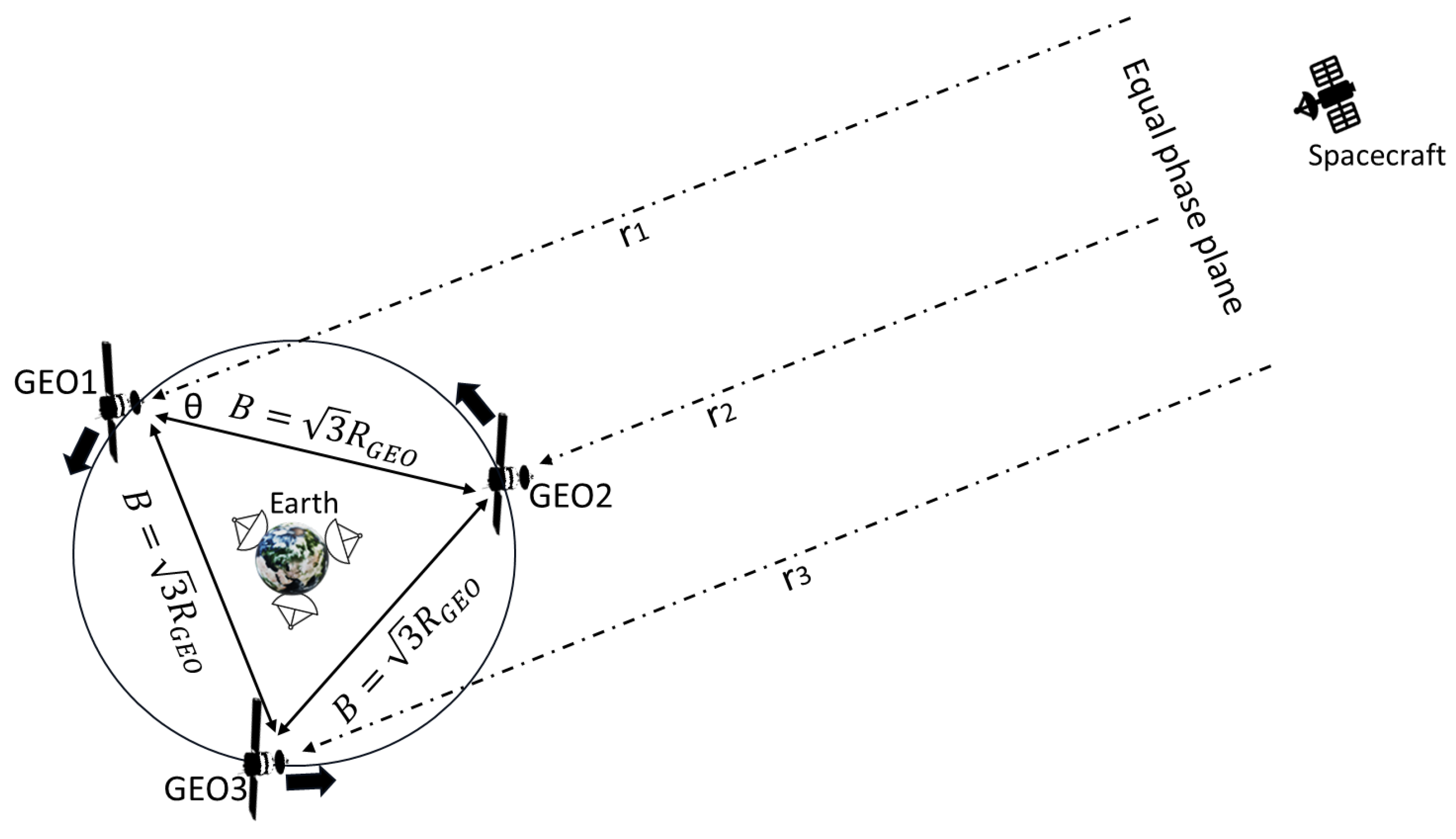
Figure 2.
Two-way time and frequency transfer implemented in the RINGS system using a bidirectional inter-satellite link.
Figure 2.
Two-way time and frequency transfer implemented in the RINGS system using a bidirectional inter-satellite link.
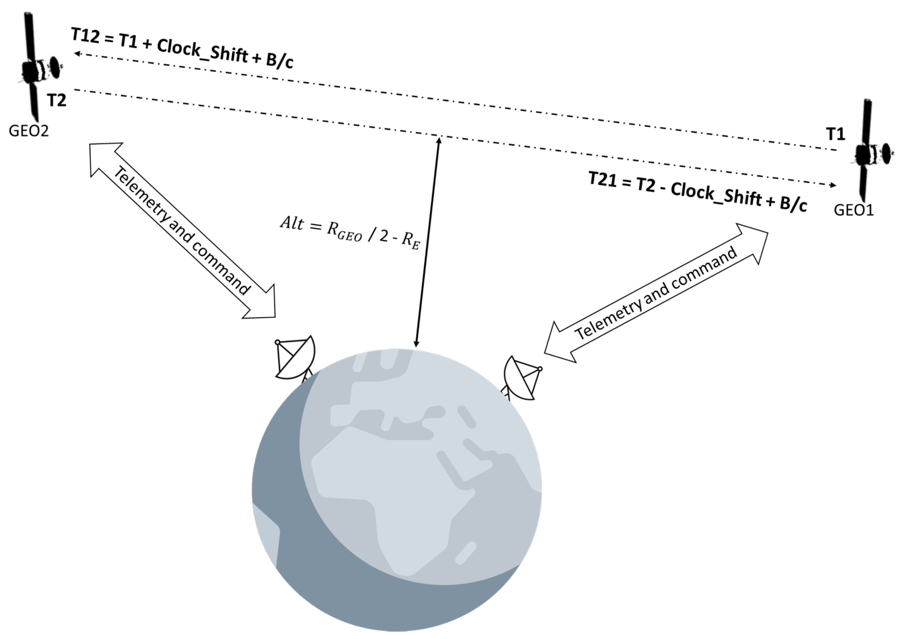
Figure 3.
RINGS simulation-based performance-analysis flow.
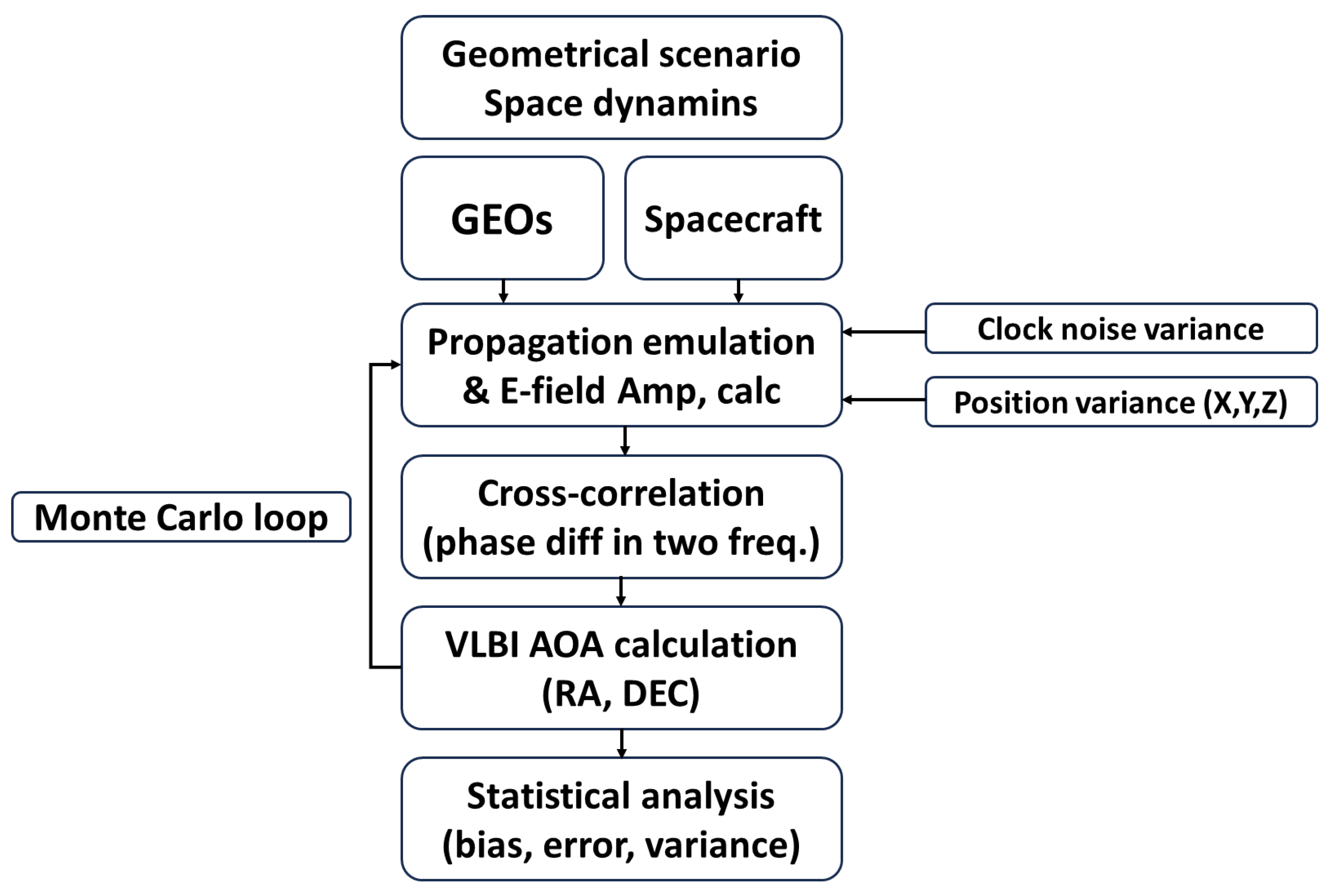
Figure 4.
Clock-only averaged AOA sensitivity. The upper panel shows the mean AOA standard deviation over the arc as a function of residual relative clock misalignment. The lower panel shows the residual from a linear fit.
Figure 4.
Clock-only averaged AOA sensitivity. The upper panel shows the mean AOA standard deviation over the arc as a function of residual relative clock misalignment. The lower panel shows the residual from a linear fit.
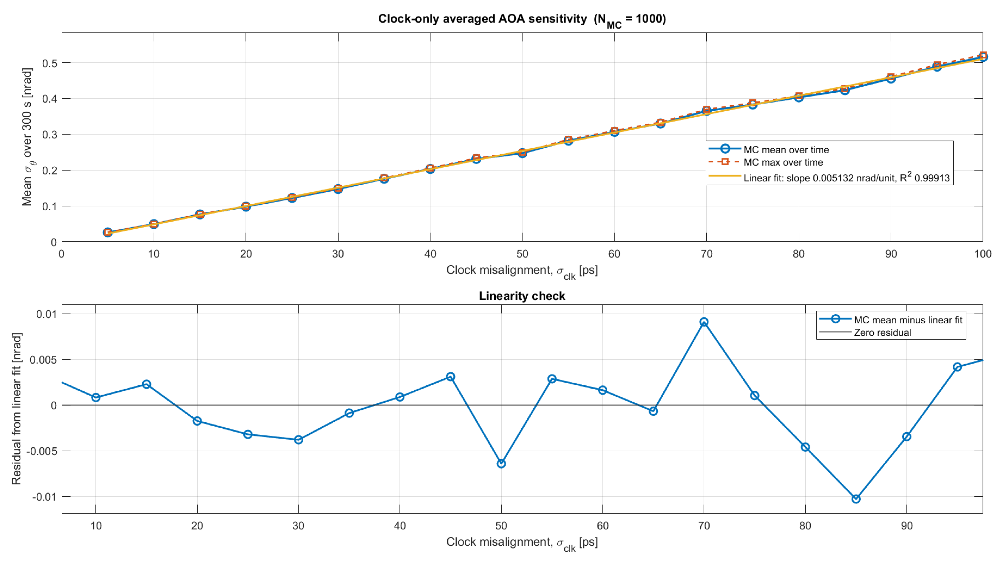
Figure 5.
RINGS AOA reconstruction for the high-accuracy case of per-axis GEO position uncertainty and clock misalignment.
Figure 5.
RINGS AOA reconstruction for the high-accuracy case of per-axis GEO position uncertainty and clock misalignment.
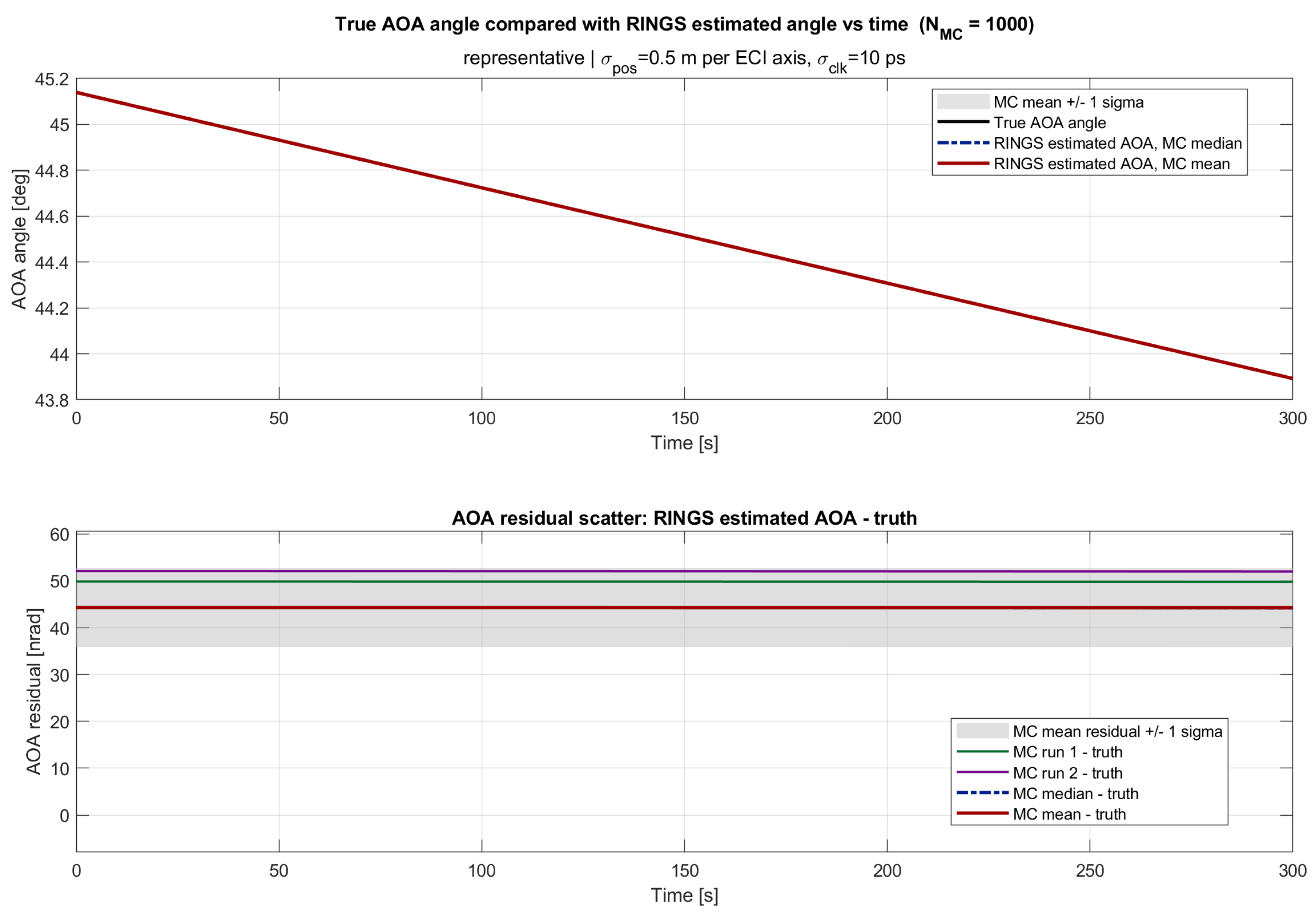
Figure 6.
RINGS AOA reconstruction for the conservative case of per-axis GEO position uncertainty and clock misalignment.
Figure 6.
RINGS AOA reconstruction for the conservative case of per-axis GEO position uncertainty and clock misalignment.
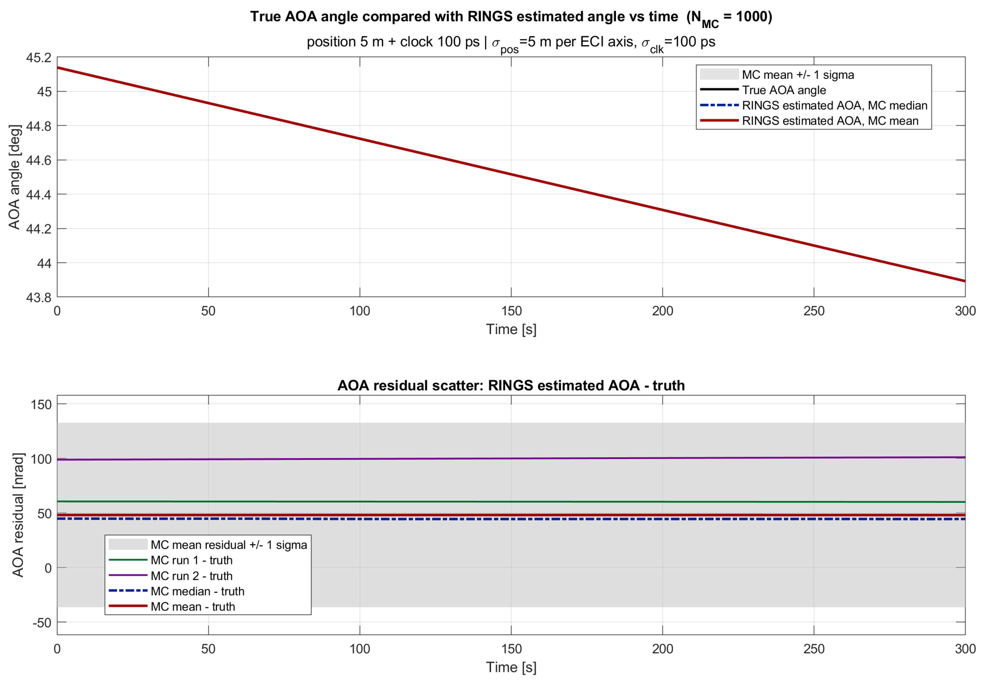
Figure 7.
RMS AOA residual for each Monte Carlo run. Each point represents the RMS residual over the full arc.
Figure 7.
RMS AOA residual for each Monte Carlo run. Each point represents the RMS residual over the full arc.
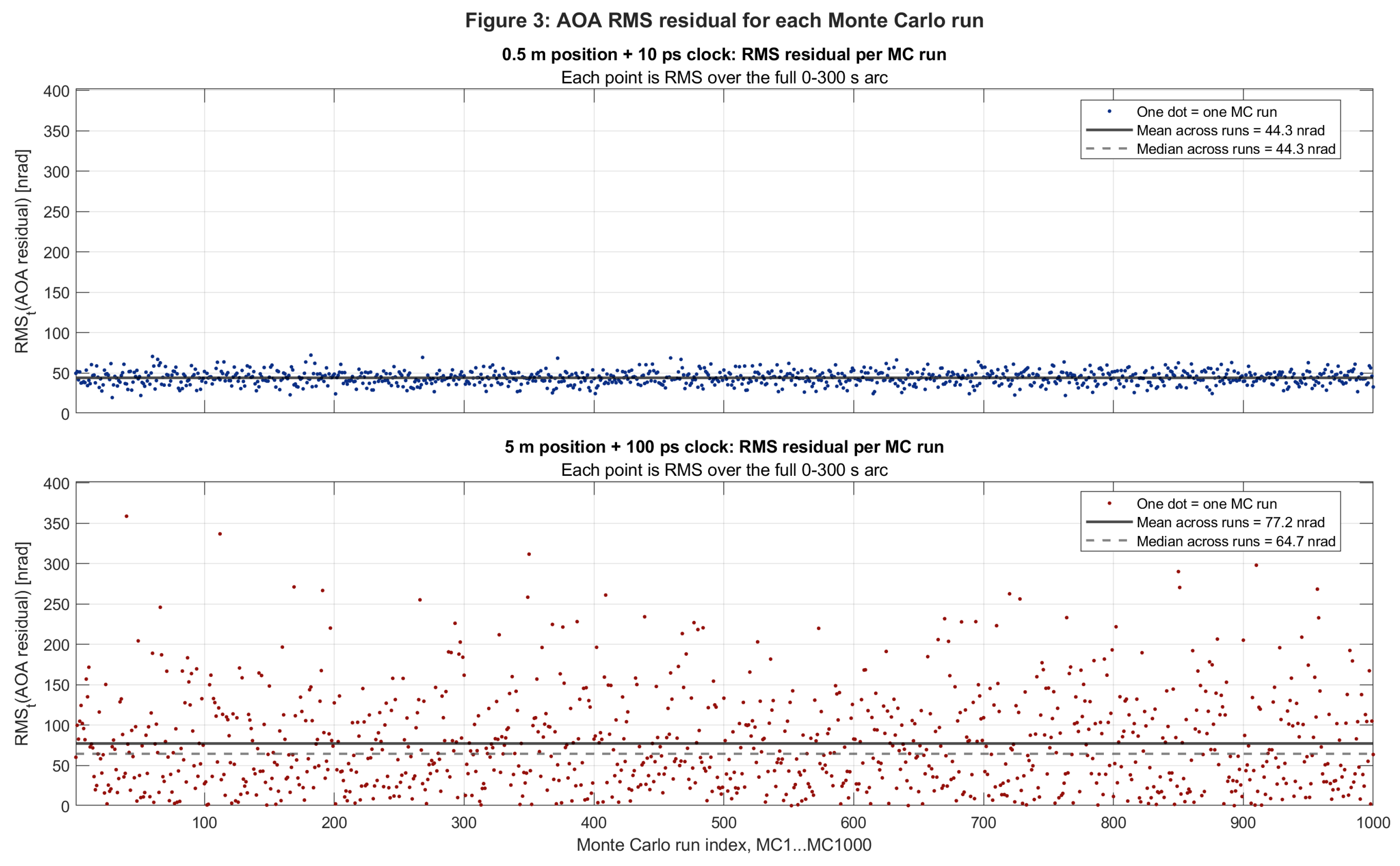
Figure 8.
Position-only averaged AOA sensitivity. The upper panel shows the mean AOA standard deviation over the arc as a function of isotropic, per-axis GEO position uncertainty in the ECI frame. The lower panel shows the residual from a linear fit.
Figure 8.
Position-only averaged AOA sensitivity. The upper panel shows the mean AOA standard deviation over the arc as a function of isotropic, per-axis GEO position uncertainty in the ECI frame. The lower panel shows the residual from a linear fit.
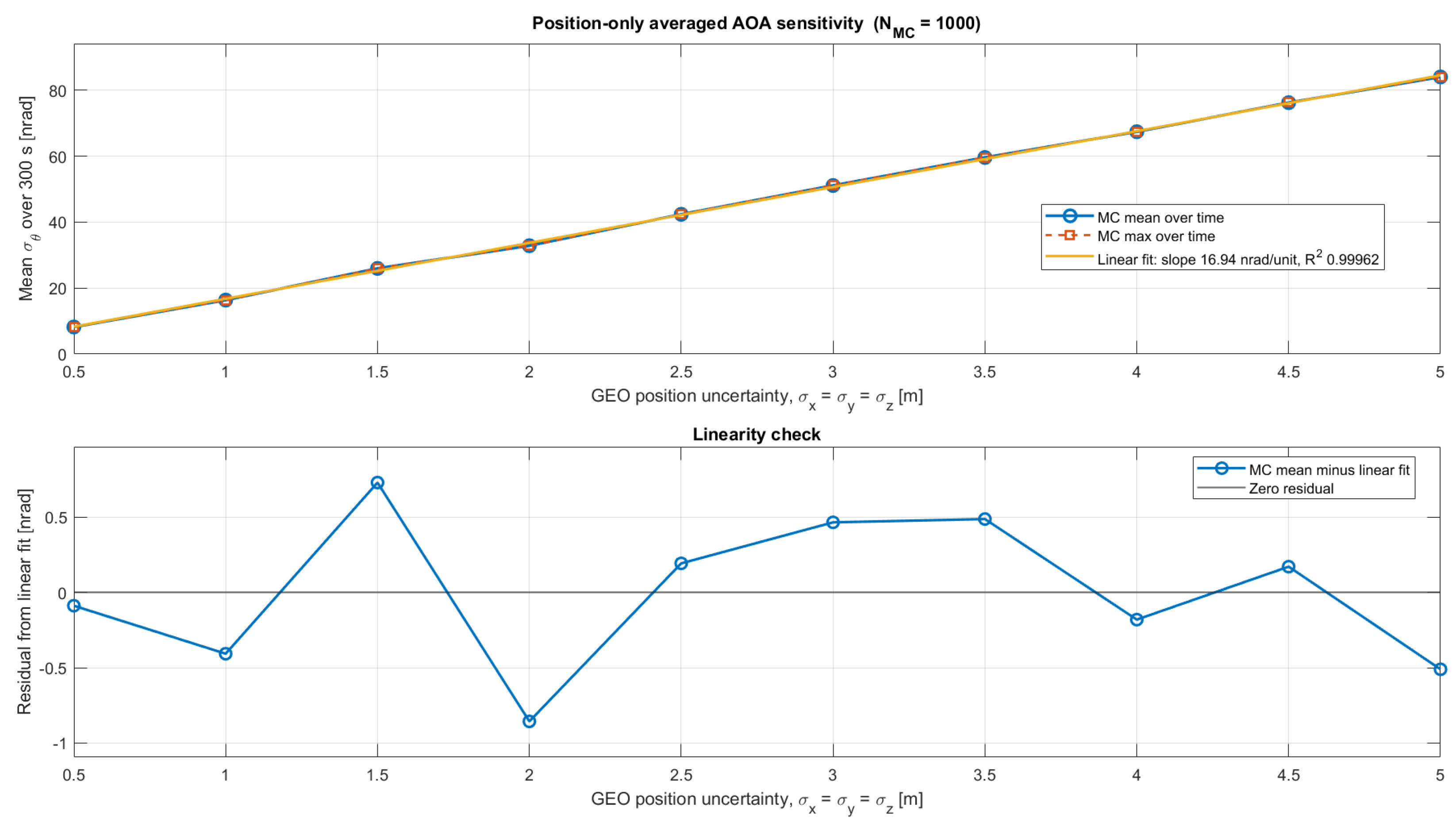
Figure 9.
Zoomed-in combined AOA sensitivity at low GEO position uncertainty.
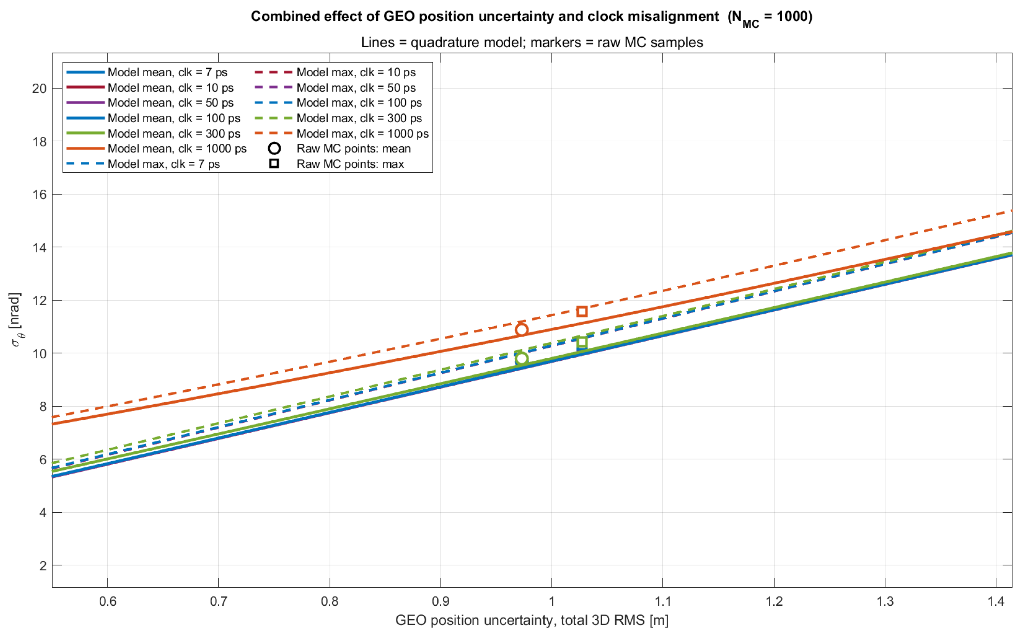

Table 1.
Allan deviation values for a space-qualified Mini-PHM-class passive hydrogen maser.
| Averaging time [s] | Allan deviation |
|---|---|
| 1 | |
| 10 | |
| 100 | |
| 1000 | |
| 10000 | |
| 50000 |
Table 2.
Analytical clock contribution to angular uncertainty for terrestrial and RINGS-scale baselines.
Table 2.
Analytical clock contribution to angular uncertainty for terrestrial and RINGS-scale baselines.
| Residual clock error | Terrestrial baseline | RINGS baseline | Near-max RINGS baseline |
|---|---|---|---|
| [ps] | |||
| 10 | 0.375 | 0.041 | 0.036 |
| 30 | 1.125 | 0.123 | 0.107 |
| 100 | 3.750 | 0.411 | 0.357 |
| 300 | 11.250 | 1.233 | 1.071 |
Table 3.
Representative clock misalignment contribution to RINGS AOA scatter.
| Clock misalignment | Mean |
|---|---|
| [ps] | [nrad] |
| 7 | 0.036 |
| 10 | 0.052 |
| 50 | 0.251 |
| 100 | 0.511 |
| 300 | 1.514 |
Table 4.
Combined GEO position and clock sensitivity.
| Position RMS | Clock misalignment | Mean | Max |
|---|---|---|---|
| 3D [m] | [ps] | [nrad] | [nrad] |
| 0.5 | 10 | 4.85 | 5.14 |
| 0.5 | 100 | 4.87 | 5.18 |
| 0.5 | 1000 | 6.94 | 7.29 |
| 1.0 | 10 | 9.69 | 10.28 |
| 1.0 | 100 | 9.70 | 10.30 |
| 1.0 | 1000 | 10.88 | 11.57 |
| 2.0 | 10 | 19.38 | 20.56 |
| 2.0 | 100 | 19.39 | 20.58 |
| 2.0 | 1000 | 20.00 | 21.30 |
| 5.0 | 10 | 48.45 | 51.40 |
| 5.0 | 100 | 48.45 | 51.41 |
| 5.0 | 1000 | 48.69 | 51.78 |
Disclaimer/Publisher’s Note: The statements, opinions and data contained in all publications are solely those of the individual author(s) and contributor(s) and not of MDPI and/or the editor(s). MDPI and/or the editor(s) disclaim responsibility for any injury to people or property resulting from any ideas, methods, instructions or products referred to in the content. |
© 2026 by the authors. Licensee MDPI, Basel, Switzerland. This article is an open access article distributed under the terms and conditions of the Creative Commons Attribution (CC BY) license (http://creativecommons.org/licenses/by/4.0/).
Copyright: This open access article is published under a Creative Commons CC BY 4.0 license, which permit the free download, distribution, and reuse, provided that the author and preprint are cited in any reuse.


