

Submitted:
02 August 2026
Posted:
04 August 2026
You are already at the latest version
Abstract
We present a compact, parameter-free expression for the inverse low-energy fine-structure constant, α⁻¹(0) = 4π³ + π² + π - 1/(32π⁴) + 1/(64π⁶). It evaluates to 137.035 999 216 and agrees with the 2020 LKB precision rubidium-recoil measurement to 7.6 × 10⁻¹¹ in relative terms (<1σ). The expression is not an arbitrary construction, but emerges as the static transverse electromagnetic susceptibility derived from the relative-entropy Hessian of a published, finite-resolution, background-independent causal-diamond framework, whose spectral modular history is the canonical S³ × S¹. Its four terms represent the bulk history volume, spin-twist, waist gluing and six-direction tip defect. This note isolates the result for better discovery, independent verification, comparison and criticism. The numerical agreement is a postdiction; it does not by itself prove uniqueness or establish a physical derivation of α.
Keywords:
fine-structure constant
; analytical expression
; parameter-free formula
; precision metrology
; atom recoil
; LKB rubidium recoil
; Berkeley caesium recoil
; relative entropy
; S3 × S1
; causal diamond
; Kubo–Mori susceptibility
; spectral geometry
; semiclassical gravity
1. Purpose and Scope
The geometric expression for originates from a broader semiclassical-gravity framework published in Entropy [1]. Built on seven natural axioms organized around three basic principles (operational locality, finite modular resolution, minimal transport), the parent work establishes a relative-entropy variational principle, a Kubo–Mori response Hessian, and a matching scale . At this scale, the vector response obeys .
This nontrivial expression for , however, appears only in a companion note [2], where it was quietly presented as an epistemic test for the gauge sector. Because the expression remains hidden within that larger architectural apparatus, this note isolates it and places it where it can be discovered, checked, compared, and challenged.
2. The Analytical Expression
The static projection for the fine-structure constant proposed in [2] is
It contains only , integer powers and multiplicities, and dyadic denominators (powers of two). No continuous fit parameter enters. The four terms are:
| Channel | Term | Contribution |
| Bulk history | ||
| Spin-twist | ||
| Waist gluing | ||
| Tip defect | ||
| Sum |
While this final residue contributes only at the level, the completed sum aligns with empirical measurements down to . An asymptotic curve fit would require additional arbitrary insertions to bridge this six-order-of-magnitude gap. The absence of such a tail indicates that the response is structurally locked by the architecture, not manually calibrated.
3. Relative-Entropic Origin
In the underlying framework [1], dynamics emerge as local statistical inference rather than global time evolution. Relative entropy measures the informational cost of explaining the fixed causal-diamond boundary data with a deformed semiclassical background. At the matched KMS equilibrium reference, the second variation of this relative entropy (the Kubo–Mori Hessian) defines the local stiffness matrix of the vacuum. By Schur’s lemma and boundary symmetries, this Hessian orthogonally decouples into independent tensor (gravitational), vector (gauge) and scalar (mass) response blocks.
The gauge sector is governed by the vector block, which measures the entropic stiffness of conserved boundary currents. Quantum consistency under large gauge transformations restricts the current algebra to integer levels . Evaluating the thermal two-point function over the finite-resolution modular orbit and normalizing it against the endpoint aperture yields a constant pixel susceptibility. Matching this discrete stiffness to the canonical transverse continuum action fixes:
Because this high-scale coupling and the static low-energy susceptibility project from the same finite current inventory, their normalizations are rigidly linked.
After isolating the static transverse electromagnetic response and integrating out the internal constraints, the vector block reduces to its zero-momentum geometric projection. Because any additional term would require an extra boundary or transport structure, this projection decomposes across exactly four defining channels. Each contributes a respective volume, holonomy, capacity or closure factor, leaving only powers of [2].
Bulk history volume ().
Modular locality fixes the compact response arena to , over which the geometric trace sums all resolved modes. This dimensionless volume provides the dominant baseline stiffness, computed as the product of the volume and the modular period :
Spin-twist ().
Spin-compatible transport requires lifting rotations to their double cover, together with the associated grading. The rotational configuration space contributes the quotient volume , while antiperiodic closure around the modular circle adds the half-cycle holonomy . These are distinct spin-closure responses, not additional spacetime volume; together they encode the rotational and holonomy data required for a closed thermal fermionic loop.
Waist-gluing interface ().
Boundary completion joins the past and future light-cone halves through a closed waist. Unlike the other terms, the waist is a shared constrained interface. Eliminating this mode allows the system to relax, lowering the effective stiffness via a negative Schur-complement correction. Gauss–Bonnet fixes its scalar-curvature capacity to . Normalized against the bulk history volume , the correction factorizes as
Octahedral tip-defect closure ().
Near the past and future tips, sub-resolution geometry manifests as localized Regge-type defects. Continuous flux transport is replaced by the minimal octahedral router, whose coordination number counts six signed directions rather than three unoriented axis pairs. Both tips are already included in the closed modular history, so no extra factor of two appears. Orientation-complete closure acts multiplicatively across the six signed transport channels. Normalization by the modular period gives
These four terms are not adjustable coefficients, but closed projections of the vector Hessian onto the boundary invariants. The resulting coefficients are strictly dyadic, fixed by the underlying architecture rather than chosen via small-integer search. The geometric inventory is exhausted at the final tip-closure term .
The construction is fragile in a useful sense: periodic spin closure removes , omitting the rotational quotient removes , removing the shared waist shifts the result by , and altering the six-channel router changes the final residue. This comparison is unusually precise because is already a static susceptibility.
4. Comparison with Metrological Measurements
The two most precise atom-recoil determinations of the fine-structure constant are the 2020 LKB rubidium measurement [3] and the 2018 Berkeley caesium measurement [4], which differ by more than . Since no empirical coefficient enters the derivation, the present result discriminates between them.
| Benchmark | Rel. diff. | Std. dev. | |
| Nusbaumer (2026) [2] | — | — | |
| LKB 87Rb (2020) [3] | |||
| Berkeley 133Cs (2018) [4] | |||
| CODATA 2022 recommendation [5] | |||
| Electron inference (2023) [6] |
5. Comparison with Analytical Proposals
The following table compares this geometric result with a non-exhaustive selection of historical and recent compact expressions by their relative deviations from the LKB 2020 benchmark [3] and the CODATA 2022 recommended value [5].
| Proposal | Character | vs LKB | vs CODATA | |
| Nusbaumer (2026) [2] | -only from response | |||
| Pellis (2022) [7] | Golden-ratio expression | |||
| de Vries (2004) [8] | Implicit series in , , and e | |||
| Wyler (1969) [9] | Symmetric-domain volume |
Among the compact expressions considered here, the present formula gives the most precise agreement with LKB 2020. The Pellis expression is closest to the CODATA 2022 value. Notably, numerical proximity alone does not establish physical validity.
6. Computational Verification
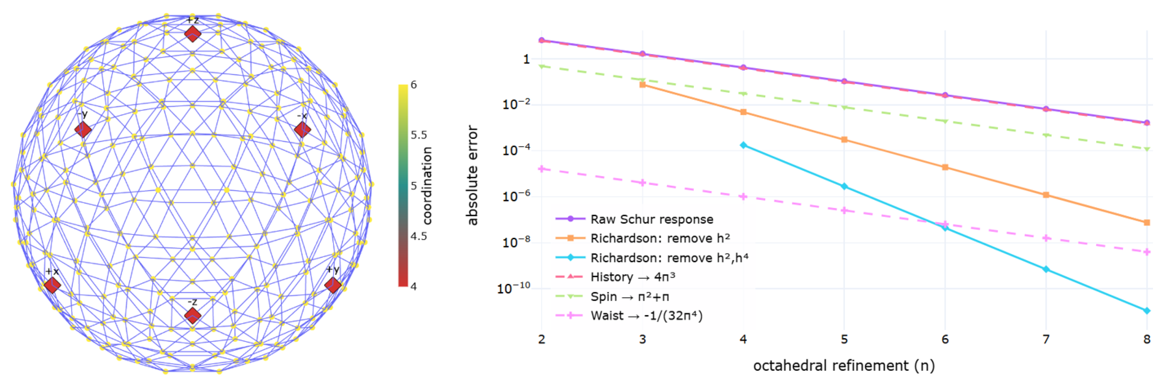
The standalone computational diagnostic fine_structure_constant.py [10] simulates the axiomatic architecture [1] on a finite mesh and tests its convergence (Figure 1). It begins with a base octahedral mesh and iteratively refines it, preserving the six transport poles at every subdivision (mesh refinement level).
The calculated mesh area generates the history and spin terms. Because the six poles are connected via local edge transport, eliminating the interior nodes collapses this network into a six-pole transition matrix. The steady state of this matrix sets the source–waist coupling, and its coherent polar factor supplies the positive tip term.
All four terms and their signs thus emerge from the framework without fitted coefficients. The waist term is a particularly clear example: its negative sign is not inserted by hand, but follows from the Schur reduction of a strictly positive source–waist Hessian. As the mesh approaches a smooth sphere, Richardson cancellation of and errors recovers the analytical expression for . At subdivision , the extrapolated response differs from the exact value by only , with no metrological input.
7. Structural Rigidity and Falsifiability
The derivation does not proceed from an integer-relation search. The four channels are evaluated from the fixed geometric and boundary constraints and then summed. No parameter is tuned.
This argument is not yet a uniqueness theorem. It does not formally exclude other geometric invariants of the same order within the admissible space. Because the physical value of was already known, the result remains a parameter-free postdiction rather than a blind prediction.
Nevertheless, the construction is structurally rigid rather than numerologically assembled. Its terms and signs emerge from the underlying axioms, requiring absolutely no metrological input.
The framework is falsifiable on three fronts. Empirically, it fails if future high-precision measurements exclude this exact value. Structurally, it fails if an independent calculation alters one of the coefficients, identifies a missing invariant, or shows that the result is regulator-dependent. Physically, it fails if the calculated static response cannot be identified with the low-energy electromagnetic coupling .
Supplementary Materials
The following supporting information can be downloaded at the website of this paper posted on Preprints.org.
References
- Nusbaumer, O. Relative-Entropy Variational Principle for Semiclassical Gravity with Finite-Resolution Boundaries. Entropy 2026, 28, 606. [Google Scholar] [CrossRef] [PubMed]
- Nusbaumer, O. Relative-Entropy Variational Principle for Semiclassical Gravity with Finite-Resolution Boundaries. Zenodo 2026, Preprint. [Google Scholar] [CrossRef]
- Morel, L.; Yao, Z.; Cladé, P.; Guellati-Khélifa, S. Determination of the fine-structure constant with an accuracy of 81 parts per trillion. Nature 2020, 588, 61–65. [Google Scholar] [CrossRef] [PubMed]
- Parker, R.H.; Yu, C.; Estey, B.; Müller, H. Measurement of the fine-structure constant as a test of the Standard Model. Science 2018, 360, 191–195. [Google Scholar] [CrossRef] [PubMed]
- Tiesinga, E.; Mohr, P.J.; Newell, D.B.; Taylor, B.N. The 2022 CODATA Recommended Values of the Fundamental Physical Constants. NIST Stand. Ref. Database 2024. [Google Scholar] [CrossRef]
- Fan, X.; Myers, T.G.; Sukra, B.A.D.; Gabrielse, G. Measurement of the Electron Magnetic Moment. Phys. Rev. Lett. 2023, 130, 071801. [Google Scholar] [CrossRef] [PubMed]
- Pellis, S. Exact Formula for the Fine-Structure Constant α in Terms of the Golden Ratio φ. SSRN Electron. J. 2022. [Google Scholar] [CrossRef]
- de Vries, H. An exact formula for the Electro Magnetic coupling constant, 2004. Online note.
- Wyler, A. L’espace symétrique du groupe des équations de Maxwell. C. R. Acad. Sci. Paris A 1969, 269, 743–745. [Google Scholar]
- Nusbaumer, O. Supplementary Simulation Toolbox for Semiclassical Gravity as Local Statistical Inference. Zenodo 2026. [Google Scholar] [CrossRef]
Figure 1.
Finite-mesh realization of the boundary response. Left: octahedral mesh generated by recursive subdivision, preserving the six degree-four transport poles as the bulk approaches coordination six. Refinement from to scales the mesh from 66 to 262,146 vertices. Right: convergence of the raw and Richardson-extrapolated responses. The history, spin, and waist contributions approach , , and ; the six-channel closure fixes the tip term at . Their sum converges to the proposed expression for .
Figure 1.
Finite-mesh realization of the boundary response. Left: octahedral mesh generated by recursive subdivision, preserving the six degree-four transport poles as the bulk approaches coordination six. Refinement from to scales the mesh from 66 to 262,146 vertices. Right: convergence of the raw and Richardson-extrapolated responses. The history, spin, and waist contributions approach , , and ; the six-channel closure fixes the tip term at . Their sum converges to the proposed expression for .
Disclaimer/Publisher’s Note: The statements, opinions and data contained in all publications are solely those of the individual author(s) and contributor(s) and not of MDPI and/or the editor(s). MDPI and/or the editor(s) disclaim responsibility for any injury to people or property resulting from any ideas, methods, instructions or products referred to in the content. |
© 2026 by the authors. Licensee MDPI, Basel, Switzerland. This article is an open access article distributed under the terms and conditions of the Creative Commons Attribution (CC BY) license (http://creativecommons.org/licenses/by/4.0/).
Copyright: This open access article is published under a Creative Commons CC BY 4.0 license, which permit the free download, distribution, and reuse, provided that the author and preprint are cited in any reuse.


