

Submitted:
31 July 2026
Posted:
04 August 2026
You are already at the latest version
Abstract
This paper presents a 3D-printed wind-tunnel model of the Active Aeroelastic Aircraft Testbed developed to support experimental flutter studies. Laboratory and wind-tunnel ground vibration tests were performed using accelerometers, high-density fiber optic strain sensing, and a motion capture system to characterize the as-built structure, recover mode shapes, and reconstruct wing deformation during testing. The measurements identified an approximately 7-Hz in-plane mode that was also found to be flutter-critical by the subsequent shaker-based analysis. Updating the finite element model to represent the actual wind-tunnel mounting compliance shifted this mode to the measured frequency and reduced the frequency errors of the first five wind-tunnel-mounted modes to about 1% or less. The characterized model and wind-tunnel response data were then used in complementary flutter-prediction workflows. Multi-output autoregressive analyses of acceleration and strain data predicted nominal flutter onset between 39.7 and 40.1 m/s, while the Parametric Flutter Margin workflow used an embedded wingtip shaker to estimate flutter at 39.5 m/s and 7.3 Hz. Supporting experimental data are publicly available. The study integrates model updating, distributed sensing, deformation reconstruction, and complementary flutter-boundary identification methods into a unified experimental workflow for flexible 3D-printed aircraft structures.
Keywords:
aeroelasticity
; ground vibration testing
; model updating
; fiber optic sensing
; motion capture
; flutter prediction
; wind tunnel testing
1. Introduction
Wind-tunnel testing and ground vibration testing (GVT) provide the experimental basis for validating aircraft structural and aeroelastic models before flight testing and certification [1,2,3,4]. These tests identify modal frequencies, damping, and mode shapes while resolving coupled bending, torsion, control-surface motion, and changes introduced by the test boundary condition [2,5]. Measurement quality therefore depends not only on sensor accuracy and bandwidth, but also on spatial observability and sensor placement across the structure [6]. Aircraft GVT campaigns can require substantial instrumentation, setup, calibration, and data-reduction effort, motivating methods that reduce test time while retaining adequate modal information [3,7]. Conventional accelerometers remain the established technology for input-output modal testing, but their discrete spatial coverage, cabling requirements, installation effort, and potential mass loading can be limiting for lightweight and highly flexible structures [2,8]. No single measurement system is optimal for all these requirements; combining acceleration, distributed strain, and optical displacement measurements can improve spatial observability and provide independent checks on the identified structural response.
Distributed fiber optic sensing offers high spatial density with relatively little added mass and has been applied to structural-dynamics measurements on aerospace components [9]. Fiber optic measurements have identified natural frequencies and operational mode shapes of a full-scale helicopter rotor blade and have been compared directly with accelerometer and finite element model results [9]. Distributed strain measurements have also been used to reconstruct the bending and twist of a full-scale aircraft wing during structural loading, with photogrammetry providing an independent displacement reference [10]. Strain-to-displacement formulations have been developed for real-time deformation prediction of flexible aerospace structures, including the Helios flying wing, with applications to shape sensing, loads monitoring, and feedback control [11]. Related studies have examined fiber Bragg grating layouts for aircraft-wing shape measurement and model-based reconstruction using inverse finite element methods [12,13,14]. These capabilities also provide a foundation for structural-condition monitoring because changes in distributed strain, reconstructed shape, or modal properties can indicate changes in the structural system, although damage detection is not addressed in the present work [15,16].
Optical displacement measurements provide complementary information because they measure structural motion without attaching transducers or cables to the test article. Photogrammetry and digital image correlation are established methods for obtaining displacement and deformation fields from calibrated images [17]. In full-scale aerospace testing, photogrammetry has been used to validate wing shapes reconstructed from distributed fiber optic strain measurements [10]. Marker-based motion capture applies the same general principle using multiple calibrated cameras and identifiable targets to obtain three-dimensional displacement histories at selected structural locations. Such measurements are particularly useful for visualizing mode shapes and time-dependent wing deformation and for validating strain-based shape reconstruction. Their limitations differ from those of bonded sensors and include camera calibration, finite field of view, marker occlusion, reflections, lighting sensitivity, and spatial resolution determined by the marker layout [10,17]. Combining optical displacement measurements with acceleration and strain data therefore increases the range of observable structural behavior while exposing source-specific uncertainty.
Taken together, prior studies establish the individual value of conventional modal instrumentation, distributed strain sensing, and optical deformation measurements, but comparatively few experimental campaigns carry the same flexible aircraft structure from as-built characterization through boundary-condition correction, aeroelastic-response measurement, deformation reconstruction, and flutter-boundary identification. There remains a need for integrated demonstrations that compare complementary sensing systems under both laboratory and installed wind-tunnel boundary conditions and then connect those measurements to model updating and independent flutter-prediction workflows. This connection is important because errors in structural boundary conditions, modal observability, or data reduction can propagate directly into aeroelastic-stability estimates.
Structural characterization ultimately supports the assessment of aeroelastic stability. Flutter prediction during testing commonly uses modal frequencies and damping identified at stable, pre-flutter conditions to evaluate and extrapolate a stability parameter [18]. Autoregressive and autoregressive moving-average models have been applied to turbulence-excited wind-tunnel responses for system identification and flutter prediction [19]. Multi-output vector autoregressive moving-average (VARMA) and vector autoregressive (VAR) formulations extend this approach by accounting for dependencies among multiple acceleration or strain channels and have been applied directly to the A3TB wind-tunnel data [20,21]. The Parametric Flutter Margin (PFM) method provides a complementary strategy in which a stabilizing parameter and controlled excitation are introduced so that the nominal flutter boundary can be inferred while the tested configuration remains stable [22,23]. For the A3TB-WT, this method was implemented using a small electromechanical shaker embedded in the wingtip [24]. The embedded shaker connects safe flutter-boundary identification with the broader objective of using onboard actuation to counter aeroelastic disturbances and suppress flutter [24,25].
The Active Aeroelastic Aircraft Testbed (A3TB) unmanned aerial vehicle (UAV) was developed as a modular, low-cost platform for flutter-identification and active flutter-control studies [26]. Its flexible, replaceable, additively manufactured wings and the design objective of placing flutter within the intended operating envelope make it suitable for evaluating structural-modeling, sensing, system-identification, and control methods on a common configuration. The A3TB wind-tunnel article (A3TB-WT) is a full-scale, half-span derivative of the flight vehicle developed to provide the controlled experimental setting used in this work. The test article and its preliminary characterization and wind-tunnel results were introduced in Ref. [27]; its geometry and relationship to the parent vehicle are described together in Section 2.
Against this background, the paper makes four connected contributions. First, it characterizes the same as-built A3TB-WT structure through laboratory and wind-tunnel-mounted GVT using accelerometers, high-density fiber optic strain sensing, and a motion capture system. Second, it traces discrepancies between the measured and predicted dynamics to the test boundary condition and updates the finite element model, including the approximately 7-Hz in-plane mode that participates in the flutter mechanism. Third, it connects the characterized model and wind-tunnel response data to independent turbulence-based VARMA/VAR and shaker-based PFM flutter-prediction workflows. Fourth, it demonstrates full-field deformation reconstruction from complementary strain and optical displacement measurements and makes the supporting experimental data publicly available. The nominal configuration was not deliberately driven through flutter; instead, the campaign progressively approached the boundary and used complementary methods to infer it from stable measurements. The wingtip-shaker configuration additionally supports the longer-term objective of active flutter suppression.
This paper is organized as follows. Section 2 relates the A3TB-WT test article to the parent vehicle and summarizes the test configurations, instrumentation, and wind-tunnel campaign. Section 3 presents the GVT results from the different measurement systems and the finite element model updates. Section 4 presents the aeroelastic tests, flutter-boundary estimates, and reconstructed wing shapes. Section 5 synthesizes the findings, practical lessons from the experimental campaign, and opportunities for future work.
2. Methodology
The A3TB is a 3-m-span flying-wing configuration with geometry similar to the Lockheed Martin X-56A Multi-Utility Technology Testbed [28]. As shown in Figure 1, its rectangular wings are swept by and have of washout from root to tip. A symmetric NACA 0012 airfoil provides structural depth without introducing an aerodynamic pitching moment at zero angle of attack. Eight trailing-edge flaperons provide control authority, and wingtip fins increase lateral stability. Reference structural and geometric details are listed in Table 1.
The parent vehicle was conceived as a reusable research platform rather than a one-off demonstrator. Additive manufacturing and detachable wing panels support rapid, economical replacement or modification of flexible wings while retaining the centerbody, propulsion, and avionics. The principal design requirements included a vehicle mass of no more than 10 kg, low-subsonic sea-level operation, maneuvers up to a load factor of 1.5, closed-loop velocity and altitude control, and trim through multiple control surfaces. These choices support repeated flutter-identification and control experiments while limiting the cost and consequence of modifying or replacing the structure.
The test article studied here, designated A3TB-WT, is a full-scale half-span derivative of the parent A3TB and retains one swept and twisted wing, four flaperons, and a wingtip fin. Figure 2 shows its geometry. The wing is printed in PA-12 Nylon segments connected by a -mm woven-carbon-fiber spar and is wrapped in polyester film that provides the aerodynamic surface and additional structural stiffness. The flight-vehicle root was replaced by a clamp adapter for attachment to the pitch and plunge apparatus (PaPA) at the wind-tunnel wall, as detailed in Section 4.1. The A3TB-WT was designed at the Technion and assembled and instrumented at the University of Michigan.
Once assembled, the A3TB-WT was characterized experimentally both in the laboratory and in its wind-tunnel-mounted condition. The A3TB-WT was instrumented with two accelerometers attached to the main and rear spars on the last wing segment before the wingtip (1.43 m along the span), a high-density fiber optic sensing (FOS) system, and infrared reflectors for a motion capture camera system (MCS), both along the entire span. The instrumentation is shown in Figure 6. The optical fibers provide strain data at 6.53-mm intervals over the front and rear spars (see Section 3.2.2), and the MCS tracks the coordinates of 32 points on the wing spars and control surfaces (see Section 3.2.3). During wind tunnel tests, a 6-axis load cell attached to the root of the wing provides root load measurements and adds to the suite of collected data.
The A3TB-WT was tested in two configurations. The nominal configuration (configuration 1) has a wingtip fin identical to that of the flying A3TB. The second configuration (configuration 2), shown in Figure 3, added a tip shaker device inside the wingtip to excite the wing for flutter prediction in support of the PFM studies [22,24].
The wind-tunnel campaign was conducted over two progressively expanded airspeed ranges for each A3TB-WT configuration. Initial envelope-assessment tests were conducted at a root angle of attack of 3 degrees over 16–26 m/s for configuration 1 and 20–28 m/s for configuration 2. These lower-speed measurements established the modal trends and stability margins used to proceed safely toward the expected flutter boundary. Testing was then extended at a root angle of attack of 5 degrees over 26–39 m/s for configuration 1 and 26–42 m/s for configuration 2. Table 2 summarizes the combined test envelopes. For configuration 1, the A3TB-WT’s basic response to tunnel turbulence was characterized, followed by individual and combined step flaperon deflections, individual and combined flaperon sine sweeps, and finally dynamic combined flaperon impulse responses at different control-surface deflection amplitudes. For configuration 2, the flaperons were actuated together at different amplitudes. These tests were followed by tip-shaker actuation using a 2-min sine sweep from 3 to 15 Hz and a short 0.2 s combined flaperon impulse. At the beginning, transition, and ending of each of these sets of tests, load cell measurements for calibration verification and GVT (with the MCS and the fiber optic system) were conducted. Table 2 provides a summary of the wind tunnel tests performed on the A3TB-WT and results from the wind tunnel tests are provided in Section 4.3. Since the shaker for configuration 2 was added at a location that increases the flutter velocity, the wind tunnel tests were conducted starting with configuration 2 first, up to 42 m/s, and then with configuration 1, up to 39 m/s.
The instrumentation and data products collected during the campaign are summarized in Table 3. The table is intended to set the scope for the model-characterization, flutter-prediction, and shape-reconstruction results discussed in the following sections.
These wind tunnel tests provided additional data close to the flutter boundary and were used to evaluate the dynamic behavior of the A3TB-WT as it approaches flutter. Overall, the tests conducted in the wind tunnel with this extensive instrumentation setup provide a large amount of static and dynamic data.
3. Structural Dynamics Characterization
3.1. Baseline Numerical Model
A detailed Nastran finite element model (FEM) that was originally created during the design of the A3TB [26] was adapted for the A3TB-WT and is shown in Figure 4. The results of the modal analysis for configurations 1) wing only (with and without skin) and 2) wing with a small wingtip shaker are given in Table 4.
3.2. Ground Vibration Tests
The GVT campaign combined impact-hammer and shaker excitations with on- and off-wing instrumentation to identify modal frequencies and mode shapes for the A3TB-WT. The response was measured using high-resolution strain-sensing optical fibers, high-sensitivity vibration accelerometers, and an MCS with multiple cameras and infrared (IR) reflective markers on the wing. The layout of the fiber-optic cables, IR markers, and accelerometers installed on the A3TB-WT wing is shown in Figure 6. This combination allowed conventional accelerometer-based modal results to be compared with distributed strain and optical displacement measurements while limiting added mass and cabling on the lightweight structure. The comparison is important because the masses of accelerometers and cables can have a non-negligible impact on the modal parameters of lightweight structures [8], whereas the FOS cable and IR markers provide complementary measurements with relatively small installation mass.
The wing was tested in both the skin-off and skin-on states to determine the impact of the skin on the natural frequencies and mode shapes as well as the ability of the detailed FEM to capture the effects of the skin. Configuration 2 was also included in the GVT to characterize the effect of the wingtip shaker. Figure 5 shows the A3TB-WT wing setup for these tests.
The different data collected during GVT are:
- 1.
- Acceleration data from high-sensitivity vibration accelerometers, shown in Section 3.2.1;
- 2.
- Strain data from fiber optic strain sensors, shown in Section 3.2.2;
- 3.
- Displacement data from motion capture system, shown in Section 3.2.3.
3.2.1. Accelerations from High-Sensitivity Vibration Accelerometers
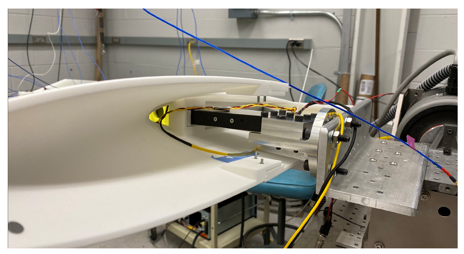
During GVT, the wing was instrumented with 16 uniaxial and 2 triaxial accelerometers. The uniaxial accelerometers were uniformly spaced over 6 stations along the span and each station had one accelerometer near the front spar and another near the rear spar to capture both out-of-plane bending and torsional vibrations. One uniaxial accelerometer was placed on each of the control surfaces to resolve the contribution of the control surfaces’ resonances to the overall structural response. The triaxial accelerometers were set up along the front spar in order to resolve the in-plane bending vibrations. The process of installing the accelerometers involves using wax to stick the accelerometer on the wing surface and routing the cable overhead using a strut to support the accelerometer cable weight to minimize its interference with the structure. It also involves setting up the geometry of the test article in the Siemens LMS Test.Lab1 software along with creating a connection between the nodes of the geometry and measurement points. It was observed that the accelerometers do not stick to the rough 3D-printed Nylon 12 surface as well as they do to metals and oven-cured composite materials. This is a potential source of error in the data collected from these sensors. t The wing was tested using both an impact hammer excitation and a shaker excitation, in which the wing was mounted on the shaker table to allow for base excitation, as shown in Figure 7. The impact hammer test was conducted with a soft rubber tip for excitation. The test software was configured to resolve frequencies up to 100 Hz. Similarly, the shaker excitation was set up as a stepped sine excitation from 2.0 Hz to 100.0 Hz with increments of 0.1 Hz and 10 cycles at each increment. The results for the natural frequencies identified using the Siemens LMS.TestLab software and the vibration accelerometers for configuration 1 with and without skin are given in Table 5. The corresponding results for configuration 2 with skin are given in Table 6.
Figure 6.
FOS layout (blue line), vibration accelerometers (red markers), and IR markers (purple and orange markers) over the A3TB-WT computer-aided design model.
Figure 6.
FOS layout (blue line), vibration accelerometers (red markers), and IR markers (purple and orange markers) over the A3TB-WT computer-aided design model.
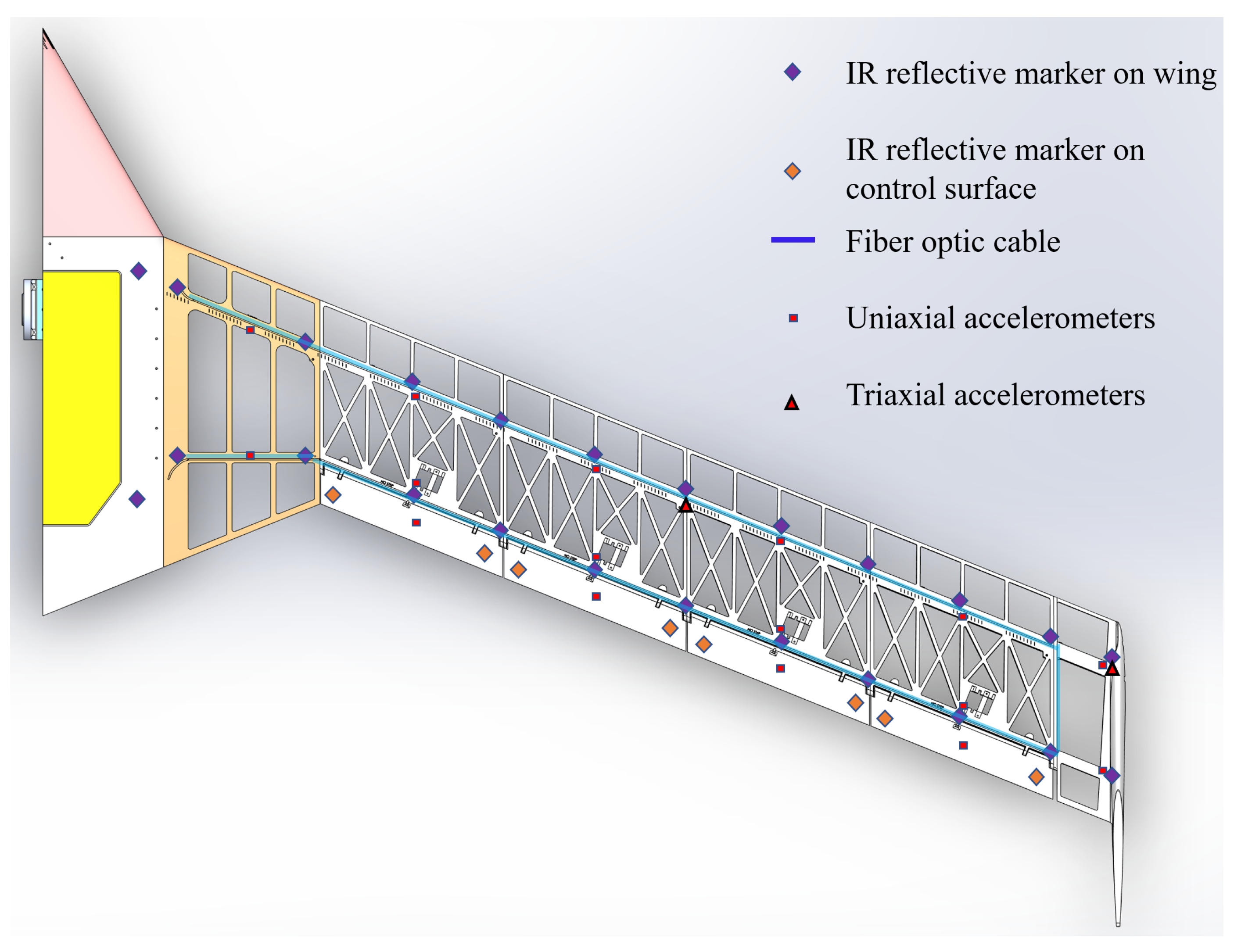
Figure 7.
The A3TB-WT model clamped to the shaker table during GVT.
The results shown in Table 5 corresponding to configuration 1 without skin are from the first round of GVT performed as a shakedown on the fully assembled wing (without the tip shaker) and did not include accelerometers measuring the in-plane response of the wing. However, all subsequent GVT performed with the LMS Test.Lab system and the vibration accelerometers included accelerometers measuring the in-plane response. Interestingly, even without accelerometers measuring the in-plane response, there was a resonant mode identified at 6.78 Hz in this test using shaker excitation. Once the skin and in-plane accelerometers were added, a first in-plane mode was identified at 7.1 Hz for the configuration 1 with skin.
Table 7 shows the comparison of the initial numerical model and the experimentally identified modal frequencies for configuration 1 of the A3TB-WT with the skin installed outside the tunnel.
These results indicate that the discrepancy between the initial FEM and the as-built A3TB-WT was mode-dependent rather than a uniform stiffness offset. The initial model overpredicted the first out-of-plane and first in-plane frequencies, while the first torsion and third out-of-plane frequencies were lower than the corresponding GVT values. These differences are attributed to uncertainties in the 3D-printed material properties, the variability of the pre-stress caused by shrinking the polyester skin over the wing, and the idealized root boundary condition in the initial model. The first in-plane mode was present in the initial FEM, but it was predicted at a substantially higher frequency than the experimentally observed mode near 7 Hz because the initial boundary condition did not represent the actual mounting region and adapter.
3.2.2. Strains from the Fiber Optic System
A single optical fiber of length 3.2 m was installed on the wing’s upper surface and provides strain data every 6.53 mm over the front and rear spars. The layout of the fiber is shown in Figure 6. The process of installing the optical fiber is similar to that of strain gauges. The surface must be prepared and the optical fiber is glued gently over the specified path. Once the installation is finished, the sensor is installed permanently with negligible impact on the rest of the structure. Attaching the fiber to a 3D-printed surface was found to be more difficult than attaching it to a metallic surface. To facilitate the alignment, a 2-mm wide groove was designed into the surface along the path where the fiber was to be installed. This groove, however, could prevent the fiber from maintaining full contact with the structure and occasionally allow it to float in the adhesive used to attach it. This is a potential source of error in the optical-fiber measurements from the A3TB-WT and an important practical consideration for future fiber optic installations.
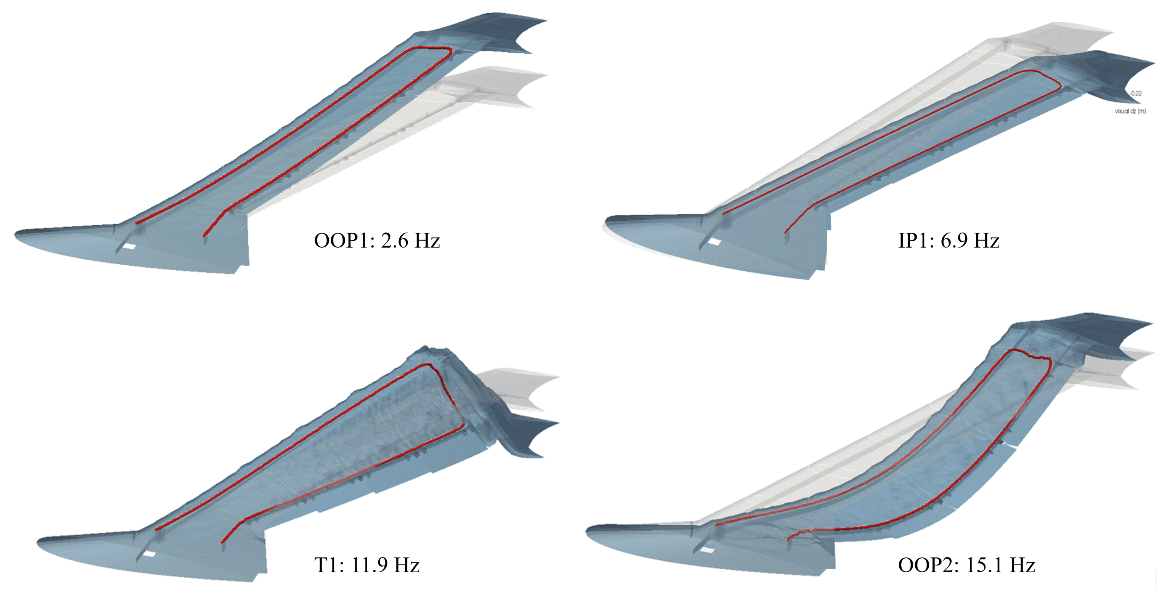
Strain data from the fiber optic system were recorded during impact GVT in both the laboratory and the wind tunnel. Each hammer impact was processed as an independent transient response: the strain channels were screened for missing or faulty measurements, baseline trends were removed, and the remaining channels were mapped to their physical locations along the leading- and trailing-edge fiber paths. Modal frequencies were identified from the spectral content of the strain response, using the fast Fourier transform (FFT) of selected channels for quick inspection and the spatially resolved response over the full fiber path to distinguish bending, torsion, and in-plane deformation. The fiber provides nearly continuous strain measurements, making it possible to resolve motion in both out-of-plane and in-plane directions from the strain measured along the leading and trailing edges. This is evident in Figure 9, where the FFT performed on the strain data indicates a resonance around 7 Hz that was also identified by the other measurement systems once the test setup included sufficient in-plane observability. Once modal frequencies are identified, the complex spectral response over the fiber path is used to extract strain mode shapes, and the strain histories can be converted to curvature and integrated along the span to estimate displacement histories and deformed shapes. The time history of an impact test recovered from the FOS point near the wingtip is shown in Figure 8. The comparison of root reconstruction assumptions in that figure shows that the recovered FOS displacement depends on how the uninstrumented root region is treated, because the fiber starts outboard of the actual wing root and the displacement integration requires an assumed root constraint. The MCS measurements described in Section 3.2.3 therefore provide an independent displacement reference for assessing the strain-based shape reconstruction. The corresponding wingtip spectrum is shown in Figure 9, and representative postprocessed FOS mode-shape visualizations are shown in Figure 10 for strain modes and Figure 11 for displacement-mode visualizations.
Figure 8.
Representative wingtip displacement time history recovered from FOS strain measurements during GVT.
Figure 8.
Representative wingtip displacement time history recovered from FOS strain measurements during GVT.
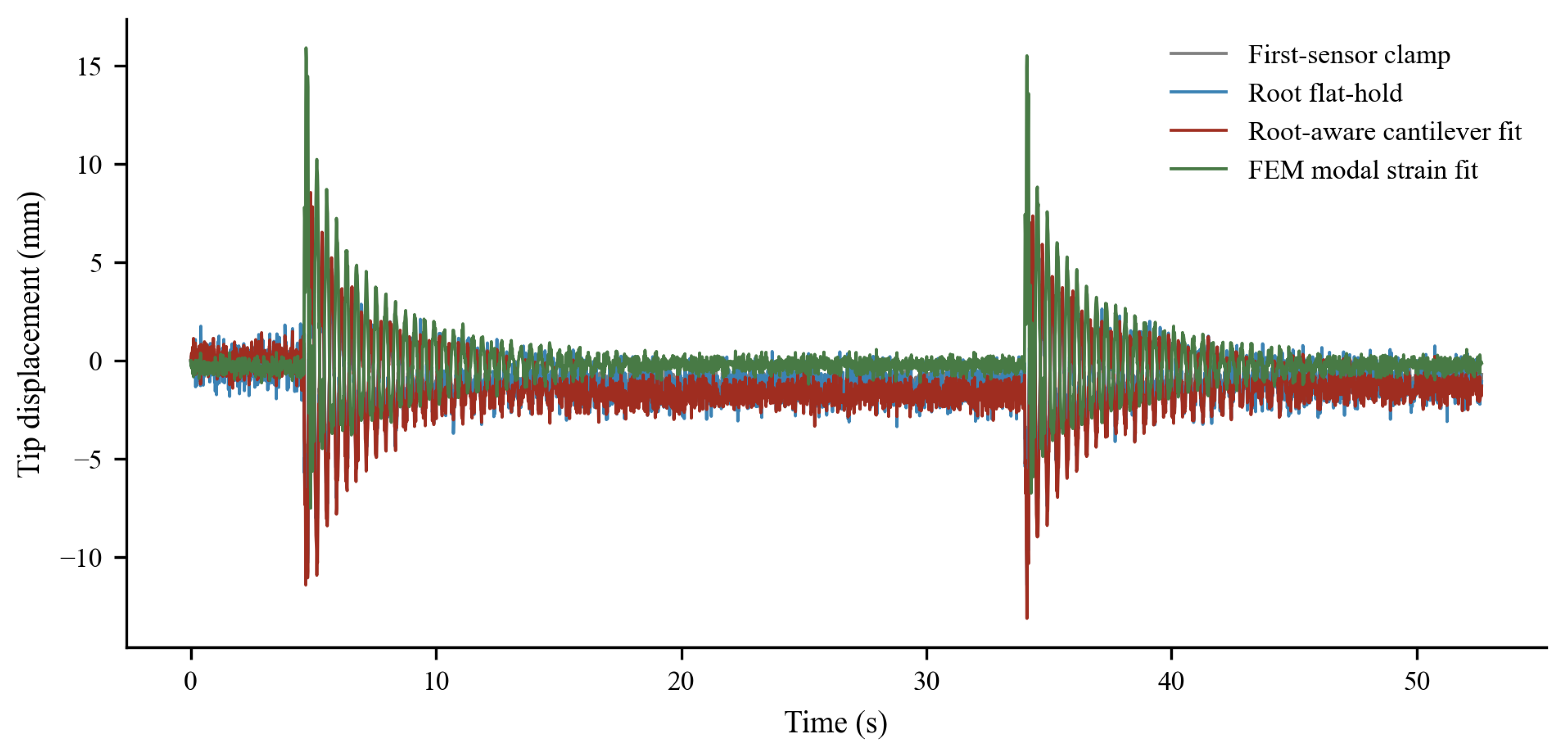
Figure 9.
FFT of the time history on the wing tip for configuration 1 recovered using the FOS data.
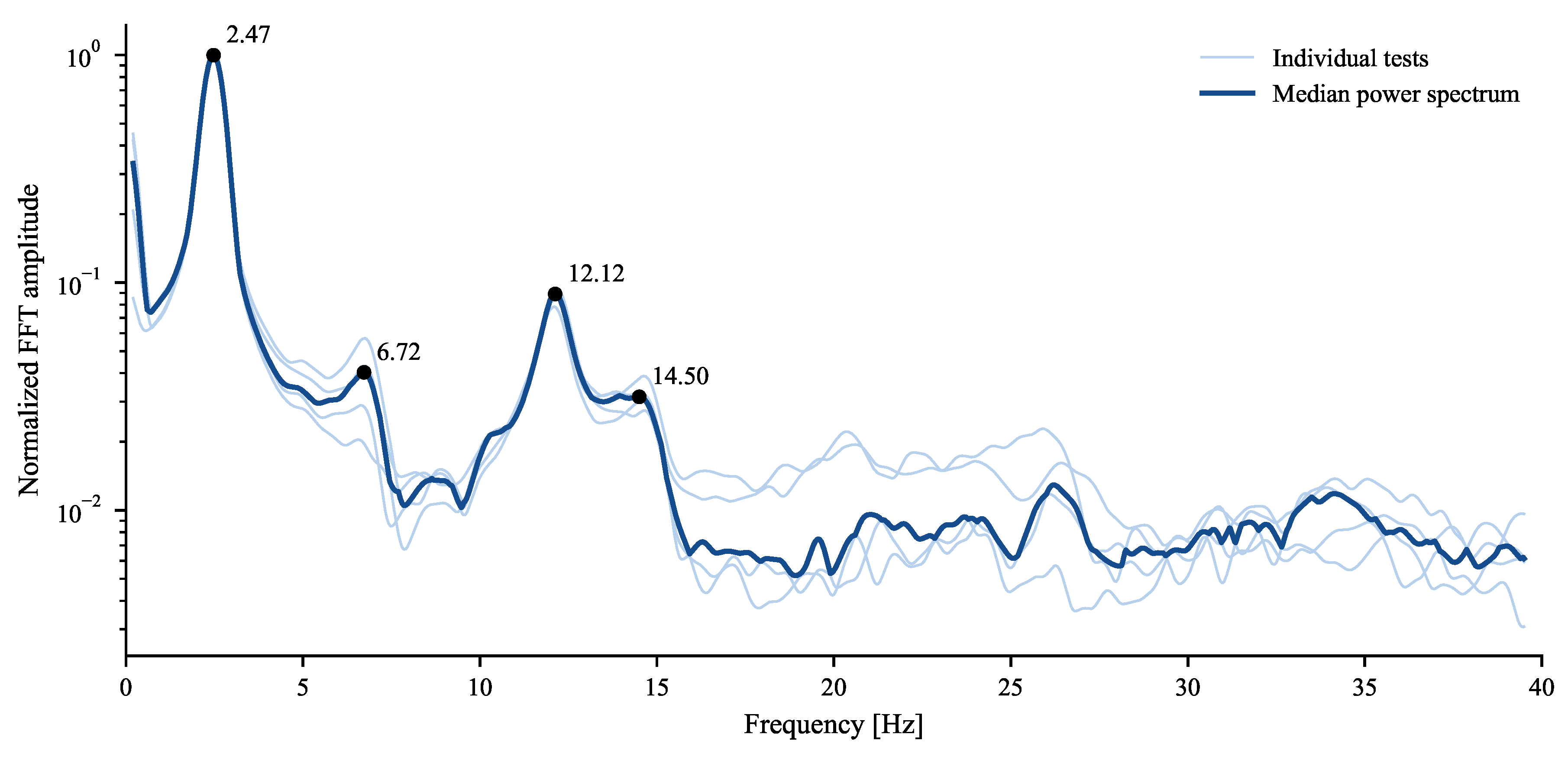
Figure 10.
Strain modes from the FOS obtained from an impact hammer GVT. Leading-edge fiber strains are shown in black and trailing-edge fiber strains in purple. First out-of-plane bending (left), first in-plane (middle), and second out-of-plane bending (right).
Figure 10.
Strain modes from the FOS obtained from an impact hammer GVT. Leading-edge fiber strains are shown in black and trailing-edge fiber strains in purple. First out-of-plane bending (left), first in-plane (middle), and second out-of-plane bending (right).
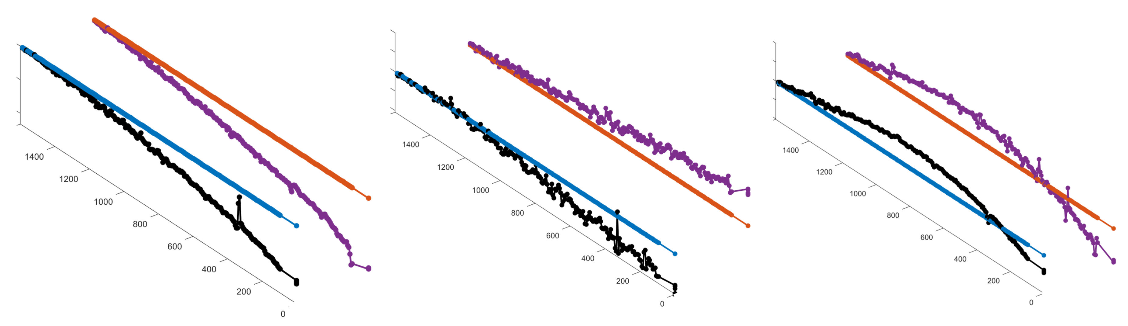
Figure 11.
First four FOS-derived mode shapes from impact GVT. Red line traces fiber optic cable as installed.
Figure 11.
First four FOS-derived mode shapes from impact GVT. Red line traces fiber optic cable as installed.
3.2.3. Displacements from the Motion Capture System
Wing deformations were captured by an OptiTrack2 motion capture system that tracks 32 infrared markers taped onto the wing, as shown in Figure 6, with a sampling rate of 240 Hz. The system measures translations in the X, Y, and Z directions, defined during the initial calibration procedure (X is in the chord-wise direction, Y is in the wing span-wise direction, and Z is the out-of-plane direction). Thirty-two infrared reflector stickers were attached to the wing along three lines:
- 1.
- Along the main spar;
- 2.
- Along the rear spar; and
- 3.
- Along the flaps at the trailing edge of the wing.
These markers were used with the MCS for both the GVT conducted in the labs as well as in the wind tunnel. The process of installing the IR markers requires attaching them at pre-specified points and is the simplest in terms of installation time and user effort compared to the vibration accelerometers or the fiber optic strain-sensing cables. However, the calibration of the motion capture system requires substantial effort to ensure the markers are captured by the cameras and do not go out of frame, where the system can lose tracking. The system is sensitive to light, and shiny objects (including floors or metallic items) can affect the quality of the calibration and, in turn, the quality of the displacement data the MCS provides. Masking sources of reflection in the capture volume requires special care during the calibration process; otherwise, marker data can be incomplete during tests. The marker trajectories were postprocessed by removing outliers, filling short gaps where possible, transforming the data from the camera calibration frame to the calibrated model axes, and applying a low-pass filter before modal analysis. The cleaned displacement histories provide direct measurements of the wing motion at the marker locations and are useful for identifying the same bending, torsion, and in-plane modes observed in the accelerometer and FOS data, including the approximately 7-Hz in-plane mode. Experimental mode shapes, described at the three marker lines, were extracted from the transient response using spectral proper orthogonal decomposition (SPOD) analysis [29]. The sparse marker-based shapes were then visualized on the wing geometry by interpolating the marker displacements or by fitting the measured response to the corresponding FEM modal basis. The representative postprocessed MCS tip displacement and mode-shape visualizations are shown in Figure 12 and Figure 13.
The comparison of the results from the different systems used during the GVT, i.e., the conventional accelerometers, the MCS, and the FOS system, is given in Table 8. All tests were conducted under laboratory conditions. The MCS and the FOS results were obtained from the impact hammer tests, and they did not record data during the shaker excitation. The results for the conventional accelerometers were obtained from both the impact hammer and shaker excitation.
3.3. FEM Updating
Four stages of the A3TB-WT model are distinguished in the following discussion. The baseline design FEM is the model adapted from the full-aircraft design model and summarized in Section 3. The physically corrected FEM incorporates measured mass and material information and a more representative root connection before numerical optimization. The laboratory-calibrated FEM is obtained by updating the physically corrected model against the shaker-table GVT. Finally, the wind-tunnel-mounted calibrated FEM carries the laboratory-calibrated structural properties forward and updates only the mounting compliance using the wind-off GVT conducted after the model was installed in the wind tunnel.
After reviewing the A3TB-WT GVT experimental setup and comparing it to the baseline design FEM and its boundary condition, an effort was made to identify the sources of error. The significant mismatch between the baseline design FEM and the GVT was attributed to:
- 1.
- An imperfectly clamped boundary condition
- 2.
- Variability in material properties of the 3D printed material
- 3.
- Unknown prestress caused by the skin shrinkage process
The following adjustments were made to obtain the physically corrected FEM before optimization:
- 1.
- The wing frame is made of Nylon 12. Its Young’s modulus was adjusted from 1.65 GPa to 1.8 GPa (material specifications provided by the 3D-printing company were different than those used in the baseline design FEM).
- 2.
- Nylon 12 material density was changed from 950 to 890 . This was done based on the measured weight of the parts.
- 3.
- In the original FEM, all nodes on the symmetry plane were clamped. For the physically corrected model, this full-face constraint was replaced by a simplified root spring connected through rigid body elements to the nodes between the spars on the fuselage and the first segment’s interface plane. At this stage, the spring admitted only out-of-plane translation; its rotational stiffness had not yet been calibrated. Another modification was to clamp the two spar nodes that connect to the load-cell adapter (see the two screws on the carbon fiber spar near the root of the A3TB-WT in Figure 7).
After these modifications, the physically corrected FEM was compared with the experiment. The results are summarized in Table 9 for configuration 1 without skin and Table 10 for configuration 1 with skin.
Although the initial physical corrections improved agreement for the first out-of-plane and torsional modes, the FEM did not reproduce the experimentally observed first in-plane-dominated mode near 7 Hz. Instead, the corresponding in-plane motion remained coupled to a torsion-dominated mode at a substantially higher frequency.
To address the remaining discrepancy, measurements of the laboratory mounting hardware were used to relocate the spar attachment points and connect them through rigid body elements to a grid point representing the clamp adapter. Translational and rotational spring components parameterized this connection, and the rotational stiffness components were treated as active design variables. This refinement shifted the first in-plane-dominated mode to approximately 7 Hz without degrading the out-of-plane- and torsion-dominated modes. The corresponding wind-tunnel-mounted representation is described separately in Section 4.2.
Figure 14.
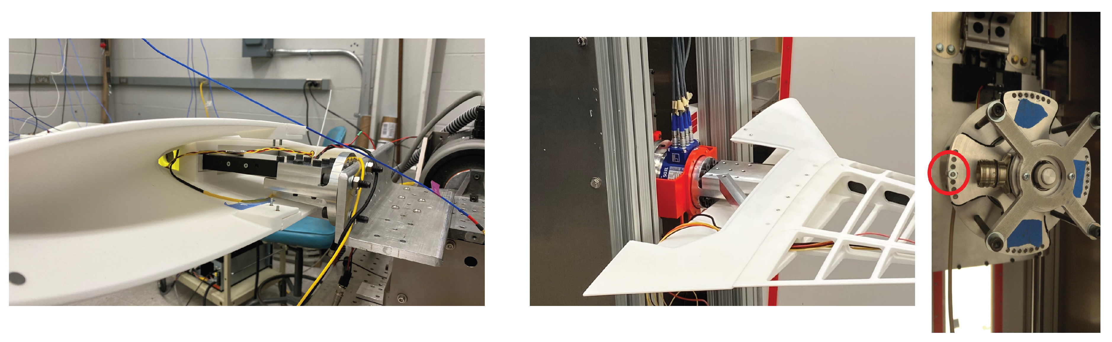
Shaker table boundary condition (left) and wind tunnel boundary condition (center and right).
Figure 14.
Shaker table boundary condition (left) and wind tunnel boundary condition (center and right).
Furthermore, a finite element model updating procedure developed by Sharqi and Cesnik [30] was modified as discussed in [31] and applied to the A3TB-WT FEM to calibrate it against the experimental GVT results. The FEM updating process is shown in Figure 15.
3.3.1. Optimization Problem: Design Variables, Bounds, and Constraints
Material properties of the different components and the root spring’s stiffness coefficients were chosen as the design variables for the A3TB-WT FEM update. Before optimization, the carbon fiber spar was characterized independently by applying static tip loads and measuring the resulting deflections. The inferred equivalent bending stiffness provided an experimentally informed starting value for the laminate properties and allowed tighter, physically defensible bounds to be imposed on the spar design variables.
The material properties were initially defined as constant along the entire structure for the respective component. Variable properties associated with the individual printed segments were also explored in Ref. [31] to represent manufacturing and joint variability. Allowing segment-dependent properties produced only a marginal improvement in the first five modal frequencies; therefore, the simpler constant-property representation was retained for the overarching calibration and aeroelastic analyses. Inequality constraints are imposed on the total mass, inertia, and center of gravity properties. The design variables have variable bounds placed on them based on the level of uncertainty in their original values. The mass- or density-related design variables have the tightest bounds since mass of individual components and the entire structure can be measured. The design variables related to the 3D-printed material and the skin stiffness were the most relaxed since those material properties are the least certain. The root spring design variables affect the in-plane bending and torsion related modes since they capture the boundary condition related to the setup of the A3TB-WT during GVT. The spring related design variables had their bounds defined based on which spring component showed the highest sensitivity to the minimization of the objective function (i.e., improved the match with the experimental results). The constraint variables had upper and lower limits set within of their original values. The design variables chosen for the optimization problem are shown in Table 11, along with their values before and after the FEM updating process.
Two calibration cases were considered, based on the different boundary conditions in the shaker-table laboratory GVT (Section 3.2.1) and the wind-off GVT in the wind tunnel (Section 4.2). The laboratory update used the natural frequencies identified from the high-sensitivity accelerometers in the frequency objective and allowed both the structural material properties and root spring properties to vary. Its results are shown in Table 12. The wind-tunnel-mounted update began from this laboratory-calibrated FEM and is discussed in Section 4.2.
4. Aeroelastic Tests
4.1. Wind Tunnel Experimental Setup
The University of Michigan’s subsonic wind tunnel was the testing facility used for this work. It features a 335-ft center-line closed return loop configuration, a 15:1 contraction ratio, and a 25-ft long, 5-ft by 7-ft test section. Airspeeds up to 76 m/s can be reached in the test section.
The A3TB-WT was mounted on the PaPA at the tunnel sidewall (see Figure 16). Although it allows pitch and plunge motions, the model was constrained in both plunge and pitch for this experiment. The PaPA setup also features its own 6-axis load cell and a rotary encoder that recorded the root angle of attack. The A3TB-WT was attached to the PaPA at its root, using holes drilled in the carbon fiber spar that are bolted into the clamp adapter that connects to the load cell onboard the PaPA, as seen in Figure 14.
The command signals to the servos controlling the flaperons were sent using a real-time Linux server running ADEPT 3 while the small wingtip shaker commands (for configuration 2) were sent using a National Instruments (NI) data acquisition (DAQ) system through LabVIEW. The NI DAQ also served as one of the main data recording devices during the tests, along with the MCS and the FOS systems. A schematic of the data flow during the wind tunnel test is shown in Figure 17.
Once the control surface deflection commands were sent to the servos, the response from the various sensors was recorded and synchronized by looping one of the control surface commands to the NI DAQ. This allowed aligning the beginning of the test (or excitation to the control surfaces) with the time stamp associated with the data being read from the accelerometers and other instrumentation in the wing and in the PaPA. A sample flaperon sweep from 1 Hz to 10 Hz conducted on configuration 2 is shown in Figure 18. The spike at the beginning of the signal is sent to allow the signal from the real-time Linux server sending control surface commands to line up with the NI DAQ and allow for time synchronization between the different systems. Similarly, the signal at the end (after 70 s) is also used to synchronize the systems.
4.2. GVT and FEM Updating in the Wind Tunnel
Once the model was assembled in the wind tunnel and mounted on the PaPA, the connection of the model’s root section to the apparatus provided a different boundary condition than the one imposed during the shaker-table GVT. The laboratory setup clamped the aluminum plate at the root of the wing (see Figure 7), whereas the PaPA locked pitch using 3-mm-diameter pins, as shown in Figure 14. The location of the central hole in the PaPA clamp adapter and the spar attachment points were measured and represented explicitly in the FEM. Rigid body elements representing the spar bolts and metallic root struts were connected to a central grid point, which was attached to ground through a six-component spring, as shown in Figure 19. This representation separates the previously calibrated structural properties from the compliance introduced by the wind-tunnel mounting hardware.
This difference in the boundary conditions necessitated performing an additional GVT with the model installed in the wind tunnel and the tunnel off. Both the MCS and FOS systems were employed for these tests. Figure 20 shows the FFT of a representative wind-off GVT time history recovered using the FOS. A comparison of the natural frequencies measured experimentally and the corresponding FEM is shown in Table 13.
The wind-tunnel-mounted calibration began from the laboratory-calibrated FEM shown in Table 12. The structural material properties were held fixed, and only the root spring components were used as design variables. The resulting changes therefore represent the compliance of the locked PaPA mounting condition rather than a second recalibration of the wing structure. The design variables and their values before and after the optimization are shown in Table 14.
The results from this FEM updating (using FOS wind-off impact GVT data as the experimental source) are shown in Table 15 and indicate errors of about 1% or less for the first five modes. This agreement applies specifically to the unloaded, wind-off configuration with the wing mounted on the locked PaPA.
4.3. Flutter Prediction from Wind Tunnel Tests
4.3.1. Aeroelastic System Parameter Identification and Flutter Prediction
The measured OOP accelerations in the two wingtip accelerometers and the strain data in response to the random turbulence excitation in the wind tunnel were used to assess the aeroelastic system’s frequencies and modal damping ratios at safe airspeeds, remote from flutter onset. The modal frequencies and damping ratios were used to evaluate the Flutter Margin (FM), representing the amount of stability left in the system at each airspeed [18]. For a two-degree-of-freedom (2-DOF) flutter, under some assumptions, the FM reduces quadratically with dynamic pressure. Thus, fitting a quadratic trend line to the data and extrapolating it to provides an estimate of flutter onset dynamic pressure (i.e., the speed at which the system has zero FM). The FM is computed from the aeroelastic system’s frequencies and damping ratios at the tested pre-flutter airspeeds. The accuracy of the flutter estimate from the FM depends on the quality of system identification and the accuracy of the estimated modal parameters.
For system identification, Ref. [21] modeled the test-recorded acceleration and strain responses using multi-output autoregressive models applied to the A3TB-WT wind-tunnel data. In the VARMA formulation, the structural responses are driven by past values of the responses and by the turbulence excitation in the wind tunnel. Compared with independent single-output autoregressive moving-average (ARMA) models, the VARMA model accounts for the mutual dependencies between the measured responses and avoids averaging modal parameters identified separately from individual sensors [19]. The same companion study also considered VAR models fitted to the correlation functions of the filtered data. The VAR approach is computationally more compact, but produces more closely spaced roots and therefore makes mode tracking more challenging, particularly for the large FOS data sets. The full parameter-identification and mode-tracking details are given in Ref. [21]. Here, we summarize the workflow and the resulting flutter predictions to show how the A3TB-WT data support multiple flutter-identification approaches. The VARMA model is expressed as
where is the vector of responses at time n, p and q are the autoregressive and moving-average orders, respectively, and and are the coefficient matrices to be estimated.
The coefficient matrices of the VARMA models are estimated by fitting the recorded data at each airspeed. The response model in Eq. 1 is written in state-space form using a companion matrix. If is an eigenvalue of the discrete-time companion matrix and is the sampling interval, then, assuming small modal damping, the circular frequency and damping ratio are obtained as [21]
The figures report the cyclic frequency in hertz and modal damping as in percent. The stability of the system at each airspeed is evaluated by the FM stability parameter [18], computed as
where
where and are the identified circular frequency and damping ratio of the two aeroelastic branches used to evaluate the FM. The FM is computed at the tested airspeeds and extrapolated to zero for flutter prediction. Although the classical FM is evaluated using two tracked branches, the PFM and higher-order VARMA analyses indicate a three-mode mechanism at higher airspeeds. The approximately 7-Hz fore-and-aft, or in-plane, mode couples with the first OOP bending and first torsion modes, and the identified aeroelastic modes contain varying contributions from all three structural modes [21,24]. The GVT-identified in-plane mode therefore participates in the flutter mechanism through this modal coupling rather than as an isolated in-plane flutter mode.
System identification and flutter prediction were based on accelerometer and FOS strain data [21]. We present here the strain-based prediction as a representative high-density sensing result. The FOS measured axial strain at 211 and 170 points over the main and rear spars, respectively, with a sampling rate of 80 Hz. Some faulty strain sensors had to be removed from the data before using it for system identification. Additionally, since the VARMA method solves an eigenvalue problem of dimensions equal to the number of sensors times the model order, the size of the data had to be reduced.
The strain data were cleaned and reduced by examining the time correlation between spatially close sensors. The front spar sensors were divided into groups of five sensors, with 50% overlap, and the time correlations between sensors in each group were computed. Since the sensors in each group are spatially close, their time data are expected to be similar, and their correlation should be high. Sensors with low correlation are likely faulty and were removed. After cleaning the data, tens of sensor channels remained at each airspeed. To avoid an excessively large problem size, only 20 sensors were used at each airspeed from different locations on the two spars.
Figure 21 shows the estimated frequencies (left), modal damping ratios (middle), and FM stability parameter (right). The mode numbering follows Ref. [21]: Modes 1 and 2 are the two flutter-critical branches that originate as the first OOP bending and first torsion modes, respectively, while Mode 4 is the tracked second OOP bending branch. The FM is evaluated using only Modes 1 and 2.
As summarized in Section 2, the flutter-prediction campaign progressively expanded the test envelope. The lower-speed measurements at a 3-degree root angle of attack were used to estimate modal trends and obtain an initial flutter-margin extrapolation while remaining well inside the expected stable envelope. That extrapolation indicated sufficient margin to proceed to the higher-speed measurements at a 5-degree root angle of attack. These additional data extended the test envelope closer to the predicted flutter boundary and allowed the FM trend to be recomputed; strain data were available up to 34 m/s in the higher-speed range.
The estimated frequencies vary smoothly with airspeed. The first OOP bending branch increases slightly in frequency, while the flutter-critical torsion-dominated branch decreases in frequency with increasing airspeed. Both branches remain stable throughout the measured airspeed range, with increasing modal damping. This indicates that the flutter of this configuration might be explosive, with damping that switches from positive to negative only very close to flutter onset.
The right panel of Figure 21 shows the stability parameter values at the tested airspeeds. The dashed line is the quadratic trend line for the lower-speed FM values over 16–26 m/s. Based on this trend line, flutter onset was estimated at 34 m/s, motivating the higher-speed portion of the campaign. Based on the FM quadratic trend line for the higher-speed strain data over 28–34 m/s, flutter is predicted at 40.1 m/s. A similar onset prediction of 39.7 m/s was obtained from the acceleration data using the VARMA workflow [21]. VAR models based on correlated acceleration or strain data provided similar trends, with somewhat less smooth damping estimates and slightly higher flutter-onset estimates depending on the data set and mode-tracking choices. The agreement among the acceleration- and strain-based predictions is important for the present paper because it shows that the instrumentation and model-characterization campaign produced data suitable for independent flutter-prediction workflows.
The acceleration-based VARMA analysis used the measured OOP accelerations from the two wingtip accelerometers in response to random turbulence excitation to identify the aeroelastic frequencies and modal damping ratios at airspeeds within the stable regime [20,21]. Figure 22 summarizes the updated higher-speed analysis: the left panel shows the convergence of the first OOP bending and torsion-dominated branches, while the approximately 16-Hz branch remains nearly constant; the middle panel shows the identified modal damping; and the right panel extrapolates the FM to predict flutter onset at 39.7 m/s. This acceleration-based prediction is distinct from, but closely agrees with, the 39.5 m/s shaker-based PFM estimate presented below and the other workflows summarized in Table 16.
The predicted flutter was also re-evaluated with the small tip shaker and corresponding component masses added to the A3TB-WT finite element model. The results indicated that the shaker configuration increased the flutter boundary of the tested system, allowing the wing to be tested at higher speeds while still providing information about the nominal, no-shaker flutter condition. More details about the wingtip-mounted shaker study can be found in Ref. [24].
4.3.2. Evaluation of Flutter Characteristics Using the PFM Method
The application of PFM, with an added mass used as the flutter parameter and the system excited by a co-located external force, is outlined in Ref. [23]. Ref. [24] applied this approach to the A3TB-WT using the tip shaker shown in Figure 3. In this companion workflow, the shaker had two roles: the moving mass, , provided a controlled excitation over the 3–15 Hz frequency range, while the base mass, , acted as a stabilizing mass margin relative to the nominal configuration. This allowed the test article to be exercised at airspeeds above the predicted nominal flutter speed while still remaining stable in the tested configuration. The corresponding accelerations were measured at the velocity points associated with the configuration 2 test points. According to Newton’s laws, the transfer function from the excitation force to the base acceleration, multiplied by the base mass, is
where, in our case, g. It can be shown [23,24] that the nominal flutter boundary, namely that of configuration 1 without the shaker, is at the velocity and frequency pair where . The FFT of the measured moving-mass and base accelerations provides and , from which is evaluated. Bode plots of the complex provide its gain and phase variations with frequency. This analysis is therefore complementary to the VARMA/VAR approach: the VARMA/VAR workflow estimates modal parameters from turbulence-excited structural responses and extrapolates the FM, while the PFM workflow uses a controlled shaker excitation and the mass-margin transfer function to infer the nominal flutter boundary. Details regarding the instrumentation, data acquisition, and data analysis used in our test are given in Ref. [24].
The variations of gain and phase of with frequency, obtained at various velocities between 26 and 42 m/s, are shown in Figure 23. The phase-cross-over frequency points, , are first identified for each velocity in the phase (bottom) plot. The gain values at these frequencies, , are then interpolated for the velocity at which , where V is the flutter-onset velocity . The corresponding cyclic flutter frequency is .
Figure 23 shows that the nominal system is clearly stable at m/s (gain ) and unstable at m/s (gain ). The signal is noisy due to air turbulence, but adequately accurate flutter velocity and frequency values can still be interpolated to yield m/s, which is consistent with the flutter velocity identified in Section 4.3.1, and Hz. With added to the nominal system, the flutter velocity increases up to about 42 m/s, where configuration 2 is still stable because it also includes the moving mass that serves as an extra safety measure. The close agreement between the turbulence-based FM predictions and the shaker-based PFM estimate provides a useful cross-check on the wind-tunnel data set and supports the use of A3TB-WT as a common test case for flutter-identification methods.
The wingtip shaker was also used for tunnel GVT to identify frequencies and damping values using the PFM instrumentation [24]. When time-domain shape data are recorded as in Section 4.4, the and values can be combined with the FFT of the shape time history to extract the flutter mode. Ref. [32] outlines and demonstrates this process.

Table 16.
Summary of flutter-prediction workflows applied to the A3TB-WT wind-tunnel data.
| Workflow | Data and excitation | Estimated flutter condition | Role in this paper |
|---|---|---|---|
| VARMA with FM [21] | Wingtip acceleration response to tunnel turbulence | m/s | Independent acceleration-based estimate from turbulence-excited response data. |
| VARMA with FM [21] | FOS strain response to tunnel turbulence | m/s | High-density strain-based estimate using the FOS data set discussed in this paper. |
| VAR with FM [21] | Correlation functions of filtered acceleration or FOS strain data | – m/s | Compact system-identification alternative; estimates are similar but more sensitive to mode tracking. |
| PFM [23,24] | Tip-shaker moving-mass and base accelerations | m/s, Hz | Shaker-based mass-margin estimate of the nominal flutter boundary. |
4.4. Wing Shape Estimation During Wind Tunnel Testing
Wing deformations during wind tunnel tests were recovered from the FOS and MCS measurements using complementary postprocessing procedures. For the FOS data, the measured strain histories along the leading- and trailing-edge fiber paths were screened, filtered, converted to curvature, and integrated along the span to estimate the dynamic wing shape. The recovered shapes provide continuous spanwise deformation estimates and can be visualized as time histories, instantaneous deformed shapes, or animations of the reconstructed motion. For the MCS data, the calibrated marker trajectories were cleaned, transformed to the model coordinate system, and interpolated over the wing geometry to obtain sparse but direct displacement-based shape estimates. Figure 24 compares the FOS- and MCS-derived wingtip histories for representative static-hold, frequency-sweep, and impulse control-surface excitations at 26 m/s. The agreement in timing and dominant response trends confirms that the two systems capture the same wind-tunnel events, while differences in amplitude reflect the distinct measurement quantities and reconstruction assumptions: the FOS response is inferred from strain integration and root treatment, whereas the MCS response is measured directly at discrete marker locations. The postprocessing tools developed as part of this work allow us to reconstruct the wind-tunnel dynamics and play them back on the FEM mesh using FOS data (Figure 25) and separately using MCS data (Figure 26). This enables improved visualization of the aeroelastic response and provides additional context for interpreting the system-identification results from the wind-tunnel test structure.
Together, the two shape estimates provide a consistency check on the recovered dynamic response across control-surface excitations and flow conditions. Future work can combine the measurements through sensor fusion and quantify the uncertainty in the reconstructed deformation.
5. Concluding Remarks
This study demonstrated an integrated experimental workflow in which structural characterization, model updating, distributed sensing, deformation reconstruction, and complementary flutter-identification methods were applied to the same flexible wind-tunnel article. The A3TB-WT is a 3D-printed, blended-wing-body half-model developed for structural-dynamics and aeroelastic studies in the University of Michigan’s 5-ft by 7-ft wind tunnel. Laboratory and wind-tunnel-mounted GVT established the effects of the model configuration and test boundary conditions. Conventional accelerometers supplied established input-output modal-analysis results, the high-density FOS measurements resolved distributed strain and supported continuous shape reconstruction, and the MCS provided direct displacement measurements at the marker locations. Together, the structural-response data summarized in Table 3 supported characterization of the as-built structure, finite element model updating, full-field deformation reconstruction, and mutually consistent estimates of the nominal flutter boundary.
The experiments demonstrated that accurate representation of the test boundary condition was essential for model correlation. The approximately 7-Hz first in-plane mode was identified by multiple measurement systems during the laboratory and wind-tunnel-mounted GVT and was subsequently identified as a flutter-critical mode by the PFM analysis. The initial FEM contained an in-plane mode, but predicted it at a substantially different frequency because its root boundary condition clamped the entire root face rather than representing the actual mounting region and adapter. Replacing that idealized constraint with a compliant root-spring representation shifted the predicted in-plane mode to the measured frequency without degrading the principal out-of-plane and torsional modes. Updating the wind-tunnel-mounted model using the root-spring properties reduced the frequency differences for the first five modes to approximately 1% or less.
The updated structural model and wind-tunnel measurements supported several independent flutter-prediction workflows. VARMA analyses predicted nominal flutter onset at 39.7 m/s using acceleration data and 40.1 m/s using FOS strain data. The PFM analysis used a small electromechanical shaker embedded in the wingtip to provide controlled excitation and independently estimated flutter onset at 39.5 m/s and a flutter frequency of 7.3 Hz. The shaker base and moving masses increased the stability margin of the tested configuration, allowing it to remain stable to approximately 42 m/s while the nominal no-shaker flutter boundary was inferred. Beyond its role in the PFM test, the embedded shaker represents an onboard actuation concept for countering aeroelastic disturbances and supporting active flutter-suppression studies. The nominal configuration was not deliberately driven through flutter; consequently, these values are boundary estimates inferred from stable, pre-flutter measurements rather than direct observations of flutter onset. Their close agreement nevertheless provides an independent cross-check and demonstrates that the same campaign can support turbulence-based system identification, controlled-excitation flutter-margin estimation, and full-field deformation reconstruction.
The campaign also yielded practical lessons for planning similar multisensor tests. Fiber optic installation should be designed to maintain continuous contact and reliable strain transfer along the sensing path; the groove used on the A3TB-WT aided alignment but could allow portions of the fiber to float in the adhesive. Routing, bonding, and protecting the fiber and its lead cables should therefore be completed and inspected before the skin limits access. A conventional strain gauge near the root, colocated with the fiber path, would provide an independent reference strain for extrapolating across the uninstrumented root region and improve strain-based recovery of wing shape and tip displacement. For the MCS, reflections from the polyester-film skin should be masked or otherwise controlled before camera calibration, and marker visibility should be verified over the complete range of model attitudes and expected deformations. Sensor coordinates, timing references, and end-to-end channel checks should likewise be established before tunnel access becomes constrained and repeated after mounting or configuration changes.
More broadly, the comparison showed that sensor selection involves tradeoffs among installation effort, spatial resolution, directness of the measured quantity, and postprocessing maturity. Robust, repeatable processing tools are therefore as important as the sensing hardware for reducing GVT turnaround time and making large experimental data sets useful for model updating and aeroelastic interpretation. The supporting data are publicly available through the repository identified in the Data Availability Statement, providing a reusable test case for evaluating structural-characterization, deformation-reconstruction, and flutter-identification methods. Future work can extend the data-processing and visualization tools to additional excitation cases and to A3TB derivatives with coupled propulsion and aeroelastic effects.
Author Contributions
Conceptualization, B.S., C.E.S.C., D.E.R. and M.K.; Methodology, B.S., C.E.S.C., D.E.R. and M.K.; Software, B.S., D.E.R. and M.K.; Validation, B.S., C.E.S.C., D.E.R. and M.K.; Formal analysis, B.S., C.E.S.C., D.E.R. and M.K.; Investigation, B.S. and T.J.; Data curation, B.S.; Visualization, B.S.; Writing, original draft preparation, B.S.; Writing, review and editing, B.S., C.E.S.C., D.E.R. and M.K.; Supervision, C.E.S.C., D.E.R. and M.K.; Project administration, C.E.S.C., D.E.R. and M.K.; Funding acquisition, C.E.S.C., D.E.R. and M.K. D.E.R. led the VARMA-based flutter analysis, M.K. led the PFM-based flutter analysis, and T.J. supported the experimental setup and motion-capture data acquisition. All authors have read and agreed to the published version of the manuscript.
Funding
This research was funded by the D. Dan & Betty Kahn Foundation, Mega Project 2.
Institutional Review Board Statement
Not applicable.
Informed Consent Statement
Not applicable.
Data Availability Statement
The data supporting the findings of this study are publicly available in the A3TB-WT experimental data repository.
Acknowledgments
This research was funded by the D. Dan & Betty Kahn Foundation, Mega Project 2. The authors thank Drs. Braden Frigoletto, Rafael Bertolin, Guilherme Barbosa, and Thiago Versiani of the Active Aeroelasticity and Structures Research Laboratory for their support during the laboratory and wind-tunnel tests. The authors also thank Professor Matthew McCrink, Dr. Dhuree Seth, and Ross Heidersbach of The Ohio State University for their participation in and support of the wind-tunnel tests.
Conflicts of Interest
The authors declare no conflicts of interest. The funder had no role in the design of the study; collection, analysis, or interpretation of data; writing of the manuscript; or decision to publish the results.
References
- Ambur, D.; Kegelman, J.; Kilgore, W. Langley Ground Facilities and Testing in the 21st Century. In Proceedings of the 48th AIAA Aerospace Sciences Meeting Including the New Horizons Forum and Aerospace Exposition, 2010. [Google Scholar] [CrossRef]
- Ewins, D.J. Modal Testing: Theory, Practice and Application, 2 ed.; Research Studies Press: Baldock, UK, 2000. [Google Scholar]
- Peeters, B.; Debille, J.; Climent, H. Modern Solutions for Ground Vibration Testing of Small, Medium and Large Aircraft. SAE Int. J. Aerosp. 2008, 1, 732–742. [Google Scholar] [CrossRef]
- Covioli, J.V.; Coppotelli, G. Experimental and Operational Modal Analysis in Support of Modal Model Updating - A Test Case. In Proceedings of the 8th IOMAC - International Operational Modal Analysis Conference, Proceedings, October 2019; pp. 283–293. [Google Scholar]
- Maia, N.M.M.; Silva, J.M.M. Theoretical and Experimental Modal Analysis; Research Studies Press: Taunton, England, 1997. [Google Scholar]
- Kammer, D.C. Sensor Placement for On-Orbit Modal Identification and Correlation of Large Space Structures. J. Guid. Control Dyn. 1991, 14, 251–259. [Google Scholar] [CrossRef] [PubMed]
- Koksal, S.; Yildiz, E.N.; Yazicioglu, Y.; Ozgen, G.O. Minimization of Ground Vibration Test Configurations for F-16 Aircraft by Subtractive Modification. Shock Vib. 2019. [Google Scholar] [CrossRef]
- Sharqi, B.; Cesnik, C.E.S. Ground Vibration Testing on Very Flexible Aircraft. In Proceedings of the AIAA Scitech Forum, Orlando, FL, January 2020. [Google Scholar] [CrossRef]
- Weber, S.; Kissinger, T.; Chehura, E.; Staines, S.; Barrington, J.; Mullaney, K.; Fragonara, L.Z.; Petrunin, I.; James, S.; Lone, M.; et al. Application of Fibre Optic Sensing Systems to Measure Rotor Blade Structural Dynamics. Mech. Syst. Signal Process. 2021, 158, 107758. [Google Scholar] [CrossRef]
- Jutte, C.V.; Ko, W.L.; Stephens, C.A.; Bakalyar, J.A.; Richards, W.L.; Parker, A.R. Deformed Shape Calculation of a Full-Scale Wing Using Fiber Optic Strain Data from a Ground Loads Test; Technical Report NASA/TP-2011-215975; NASA Dryden Flight Research Center: Edwards, CA, 2011. [Google Scholar]
- Ko, W.L.; Richards, W.L.; Tran, V.T. Displacement Theories for In-Flight Deformed Shape Predictions of Aerospace Structures; Technical Report NASA/TP-2007-214612; Edwards, CA, NASA Dryden Flight Research Center, 2007. [Google Scholar]
- Ma, Z.; Chen, X. Fiber Bragg Gratings Sensors for Aircraft Wing Shape Measurement: Recent Applications and Technical Analysis. Sensors 2019, 19, 55. [Google Scholar] [CrossRef] [PubMed]
- Gherlone, M.; Cerracchio, P.; Mattone, M.; Di Sciuva, M.; Tessler, A. Shape Sensing of 3D Frame Structures Using an Inverse Finite Element Method. Int. J. Solids Struct. 2012, 49, 3100–3112. [Google Scholar] [CrossRef]
- Roy, R.; Tessler, A.; Surace, C.; Gherlone, M. Shape Sensing of Plate Structures Using an Inverse Finite Element Method: Investigation of Efficient Strain-Sensor Patterns. Sensors 2020, 20, 7049. [Google Scholar] [CrossRef] [PubMed]
- Raghavan, A.; Cesnik, C.E.S. Review of Guided-Wave Structural Health Monitoring. Shock Vib. Dig. 2007, 39, 91–114. [Google Scholar] [CrossRef]
- Fan, W.; Qiao, P. Vibration-Based Damage Identification Methods: A Review and Comparative Study. Struct. Health Monit. 2011, 10, 83–111. [Google Scholar]
- Sutton, M.A.; Orteu, J.J.; Schreier, H.W. Image Correlation for Shape, Motion and Deformation Measurements; Springer: New York, 2009. [Google Scholar] [CrossRef]
- Zimmerman, N.H.; Weissenburger, J.T. Prediction of Flutter Onset Speed Based on Flight Testing at Subcritical Speeds. J. Aircr. 1964, 1, 190–202. [Google Scholar] [CrossRef]
- Nahom Jidovetski, T.; Raveh, D.E.; Iovnovich, M. Wind-tunnel study of the autoregressive moving-average flutter prediction method. J. Aircr. 2019, 56, 1441–1454. [Google Scholar] [CrossRef]
- Ben-Asher, T.; Raveh, D.E. Multioutput Autoregressive Method for Aeroelastic System Identification and Flutter Prediction. In Proceedings of the Israeli Conference on Aerospace Sciences, March 2022. [Google Scholar]
- Ben-Asher, T.; Raveh, D.E. Improvements to Wind-Tunnel Flutter Prediction with Application to the Active Aeroelastic Aircraft Testbed Wind-Tunnel Model. In Proceedings of the AIAA Scitech Forum, National Harbor, MD, January 2023. [Google Scholar] [CrossRef]
- Roizner, F.; Karpel, M. Parametric Flutter Margin Method for Aeroservoelastic Stability Analysis. AIAA J. 2018, 56, 1011–1022. [Google Scholar] [CrossRef]
- Roizner, F.; Raveh, D.E.; Karpel, M. Safe Flutter Tests Using Parametric Flutter Margins. J. Aircr. 2019, 56, 228–238. [Google Scholar] [CrossRef]
- Karpel, M.; McCrink, M.; Heidersbach, R.; Seth, D. Safe Wind-Tunnel Flutter Test Using a Shaker and Mass Margins. In Proceedings of the International Forum on Aeroelasticity and Structural Dynamics, Number IFASD 2022-066. Madrid, Spain, June 2022. [Google Scholar]
- Karpel, M. Design for active flutter suppression and gust alleviation using state-space aeroelastic modeling. J. Aircr. 1982, 19, 221–227. [Google Scholar] [CrossRef] [PubMed]
- Joels, T.; Mayer, A.; Naftaly, D.; Schachter, R.; Yechiely, N.; Levi, G.; Levinson, K.; Kantor, A.; Arazani, L.; Edery-Azulay, L.; et al. Design, Analysis, and Testing of the Active Aeroelastic Aircraft Testbed (A3TB) Platform. In Proceedings of the AIAA Scitech Forum, Virtual, January 2021. [Google Scholar] [CrossRef]
- Sharqi, B.; Cesnik, C.E.S.; Joels, T.; Raveh, D.E. 3D-Printed Swept-Wing Wind Tunnel Model Characterization for Aeroelastic Studies. In Proceedings of the International Forum on Aeroelasticity and Structural Dynamics, Madrid, Spain, June 2022; p. Number IFASD 2022-079. [Google Scholar]
- Burnett, E.L.; Beranek, J.A.; Holm-Hansen, B.T.; Atkinson, C.J.; Flick, P.M. Design and Flight Test of Active Flutter Suppression on the X-56A Multi-Utility Technology Test-Bed Aircraft. Aeronaut. J. 2016. [Google Scholar] [CrossRef]
- Schmidt, O.T.; Colonius, T. Guide to Spectral Proper Orthogonal Decomposition. AIAA J. 2020, 58, 1023–1033. [Google Scholar] [CrossRef]
- Sharqi, B.; Cesnik, C.E.S. Finite Element Model Updating for Very Flexible Wings. J. Aircr. 2022, 1–14. [Google Scholar] [CrossRef]
- Sharqi, B.; Cesnik, C.E. Finite Element Model Updating of a 3D Printed Swept Wing. In Proceedings of the AIAA SciTech Forum, Orlando, FL, January 2024. [Google Scholar] [CrossRef]
- de Boer, S.; Karpel, M.; Sodja, J. Safe Flutter Determination for Wings Undergoing Large Deflections. In Proceedings of the AIAA SciTech Forum, Reno, MD, January 2023. [Google Scholar]
| 1 | |
| 2 | |
| 3 |
Figure 1.
A3TB reference geometry.
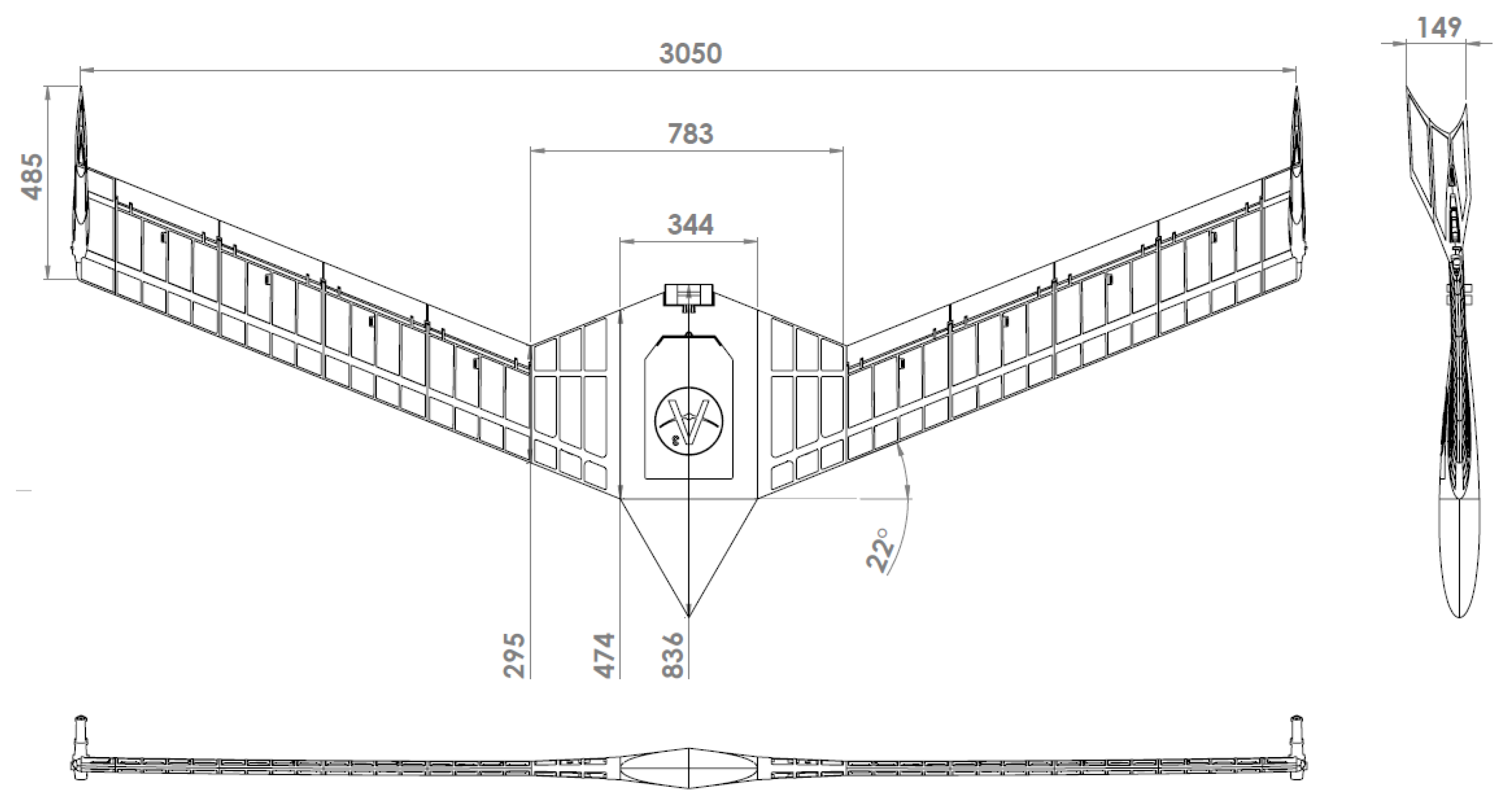
Figure 2.
A3TB-WT half-model geometry (measurements in mm). The wind tunnel apparatus is attached to the clamp adapter at the root shown at the left side of the image.
Figure 2.
A3TB-WT half-model geometry (measurements in mm). The wind tunnel apparatus is attached to the clamp adapter at the root shown at the left side of the image.
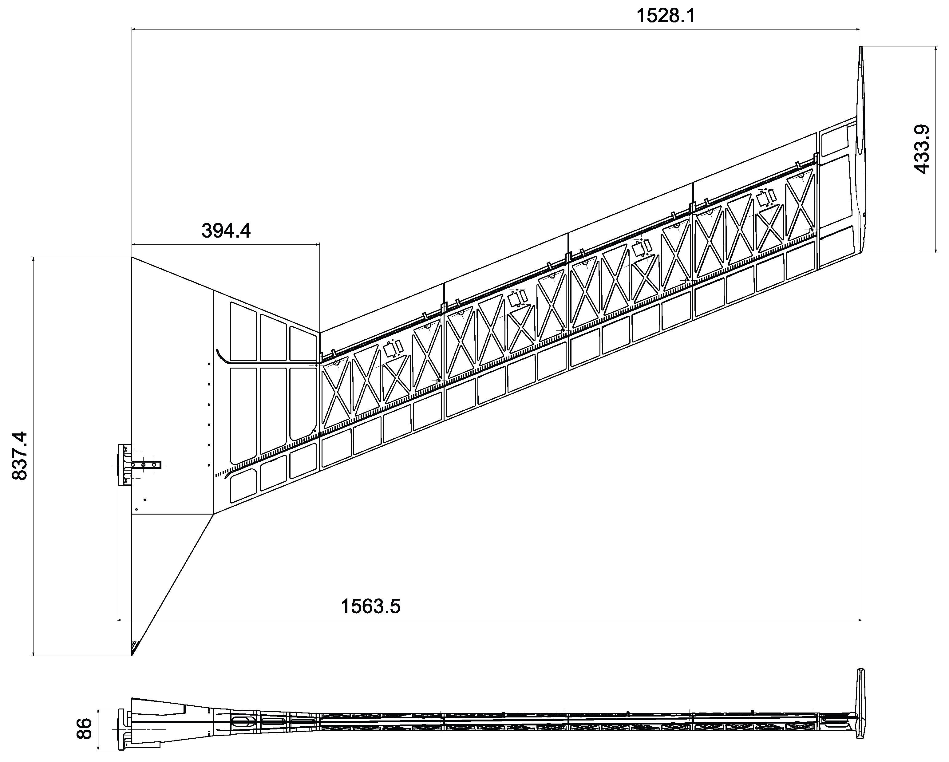
Figure 3.
A3TB-WT configuration 2 highlights (left) the housing of a small shaker at its tip, and (right) the wall-mounted arrangement in the University of Michigan 5-ft.× 7-ft. wind tunnel.
Figure 3.
A3TB-WT configuration 2 highlights (left) the housing of a small shaker at its tip, and (right) the wall-mounted arrangement in the University of Michigan 5-ft.× 7-ft. wind tunnel.
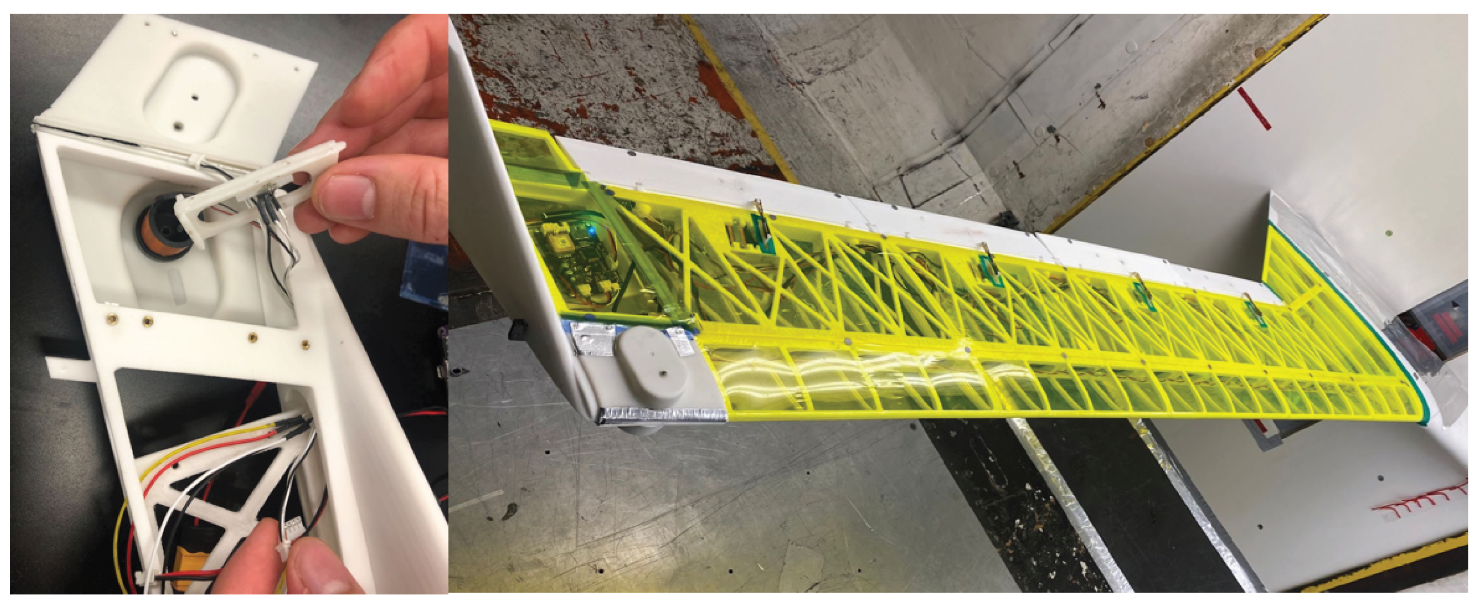
Figure 4.
Overview of the A3TB-WT FEM.
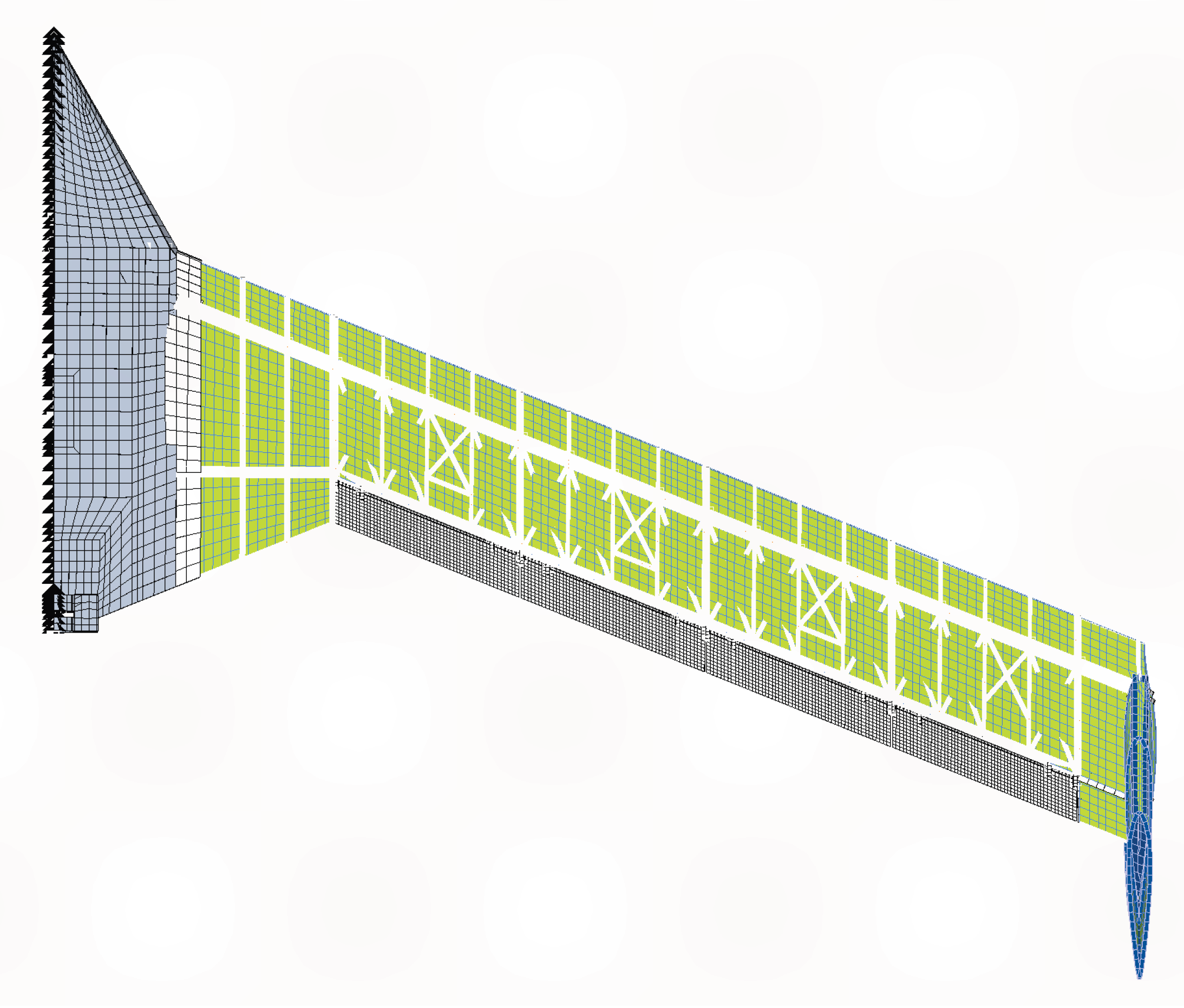
Figure 5.
Overview of the as-built A3TB-WT model without skin (left) and with skin (right) during GVT.
Figure 5.
Overview of the as-built A3TB-WT model without skin (left) and with skin (right) during GVT.
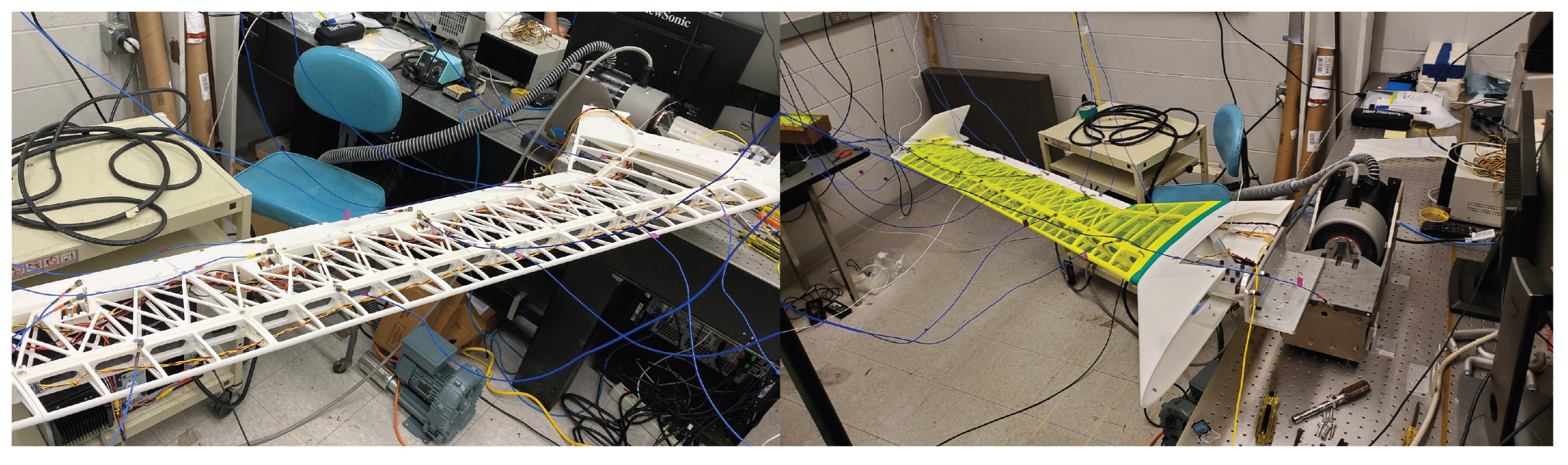
Figure 12.
Wingtip vertical displacement time history recovered from MCS marker measurements during GVT.
Figure 12.
Wingtip vertical displacement time history recovered from MCS marker measurements during GVT.
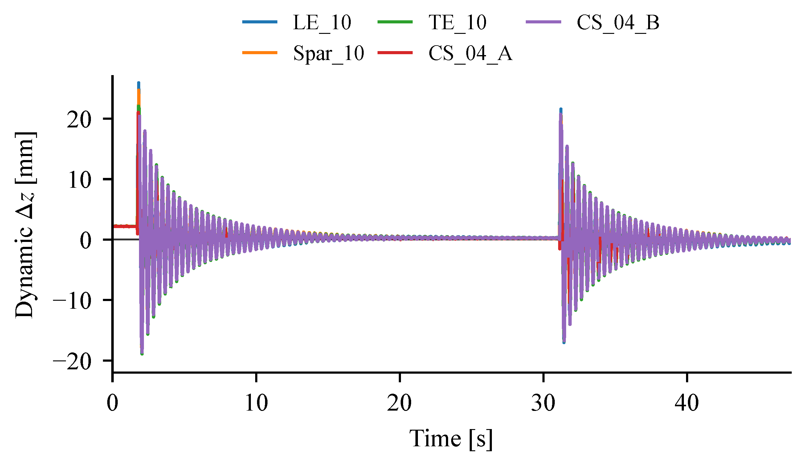
Figure 13.
First four MCS-derived mode-shape visualizations from impact GVT. Red dots indicate installed MCS markers.
Figure 13.
First four MCS-derived mode-shape visualizations from impact GVT. Red dots indicate installed MCS markers.
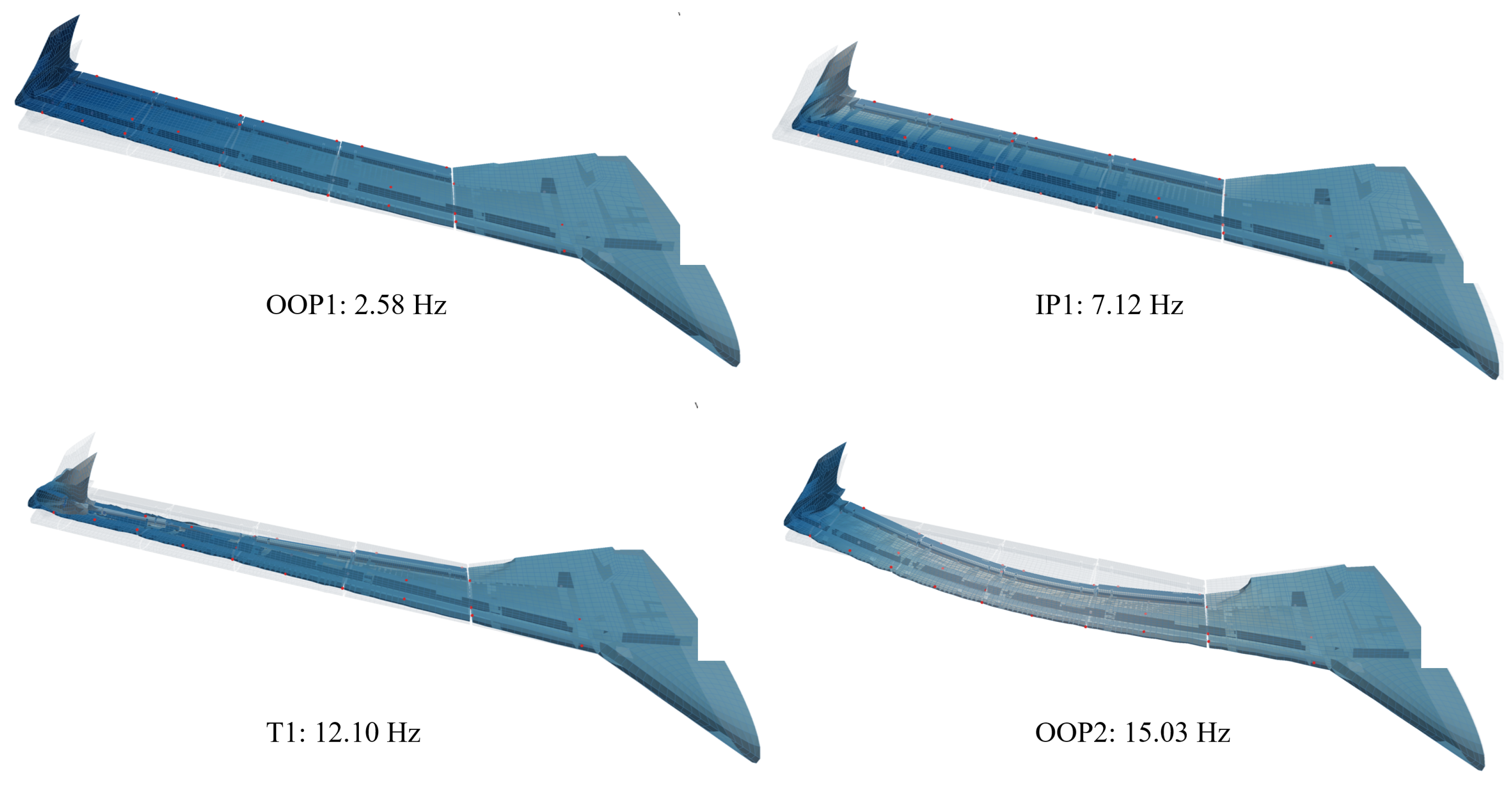
Figure 15.
Finite element model updating process modified to account for 3D-printed structures.
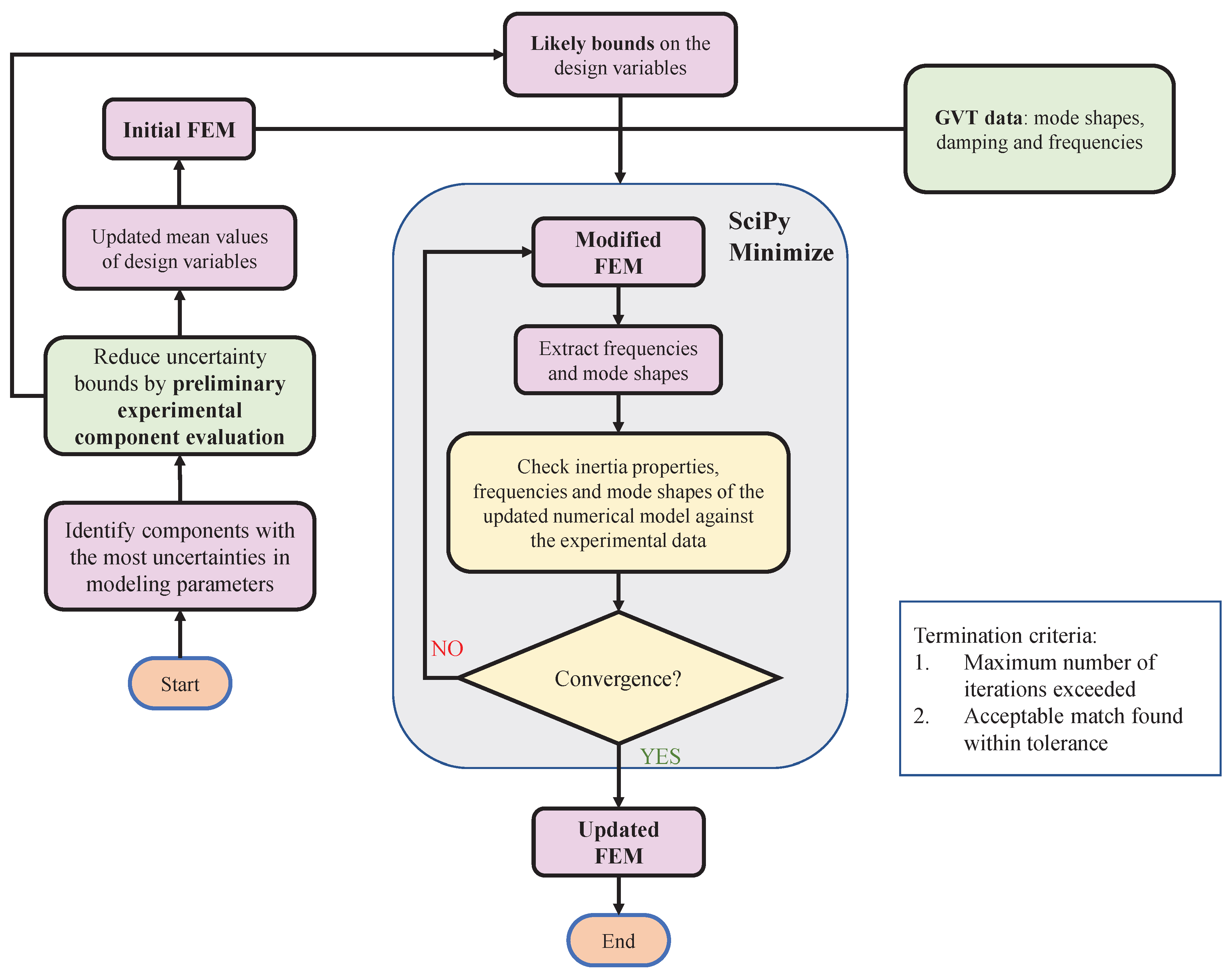
Figure 16.
Schematic of the PaPA (left) and its location in the University of Michigan 5-ft by 7-ft subsonic wind tunnel (right).
Figure 16.
Schematic of the PaPA (left) and its location in the University of Michigan 5-ft by 7-ft subsonic wind tunnel (right).
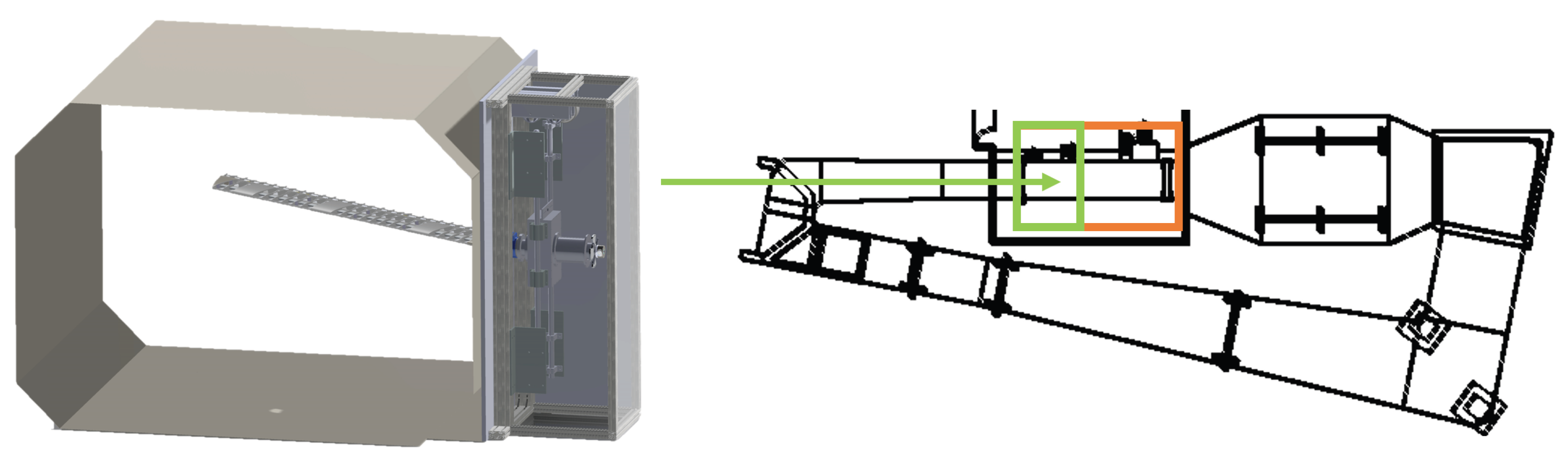
Figure 17.
Data flow during the A3TB-WT wind tunnel tests.
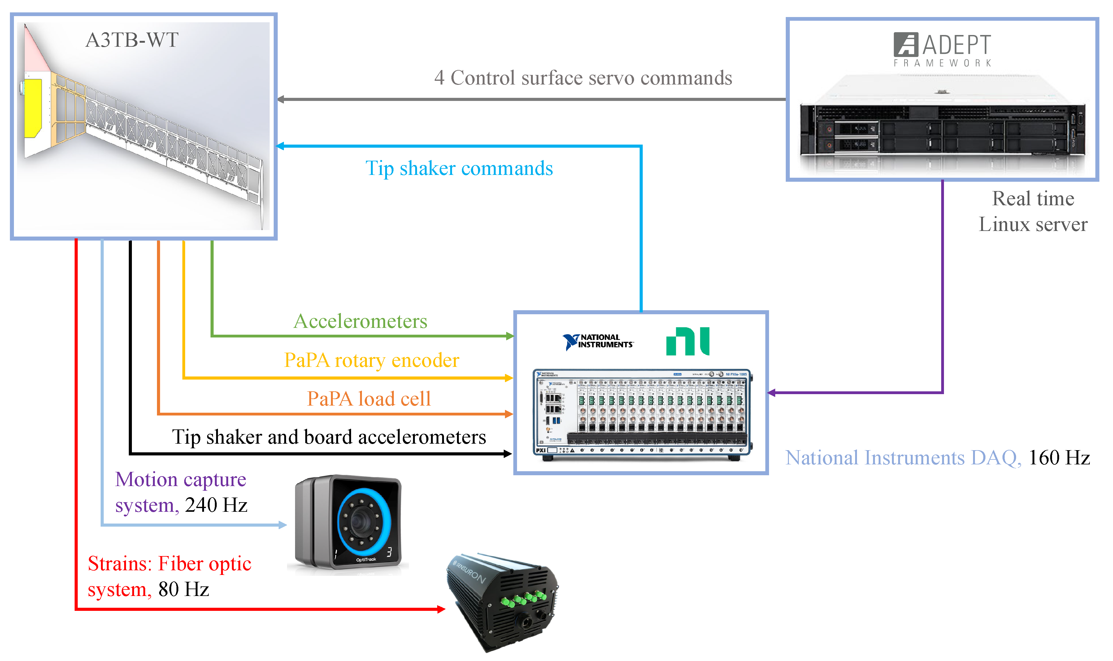
Figure 18.
Sample signal sent to control surfaces for flaperon sweep tests.
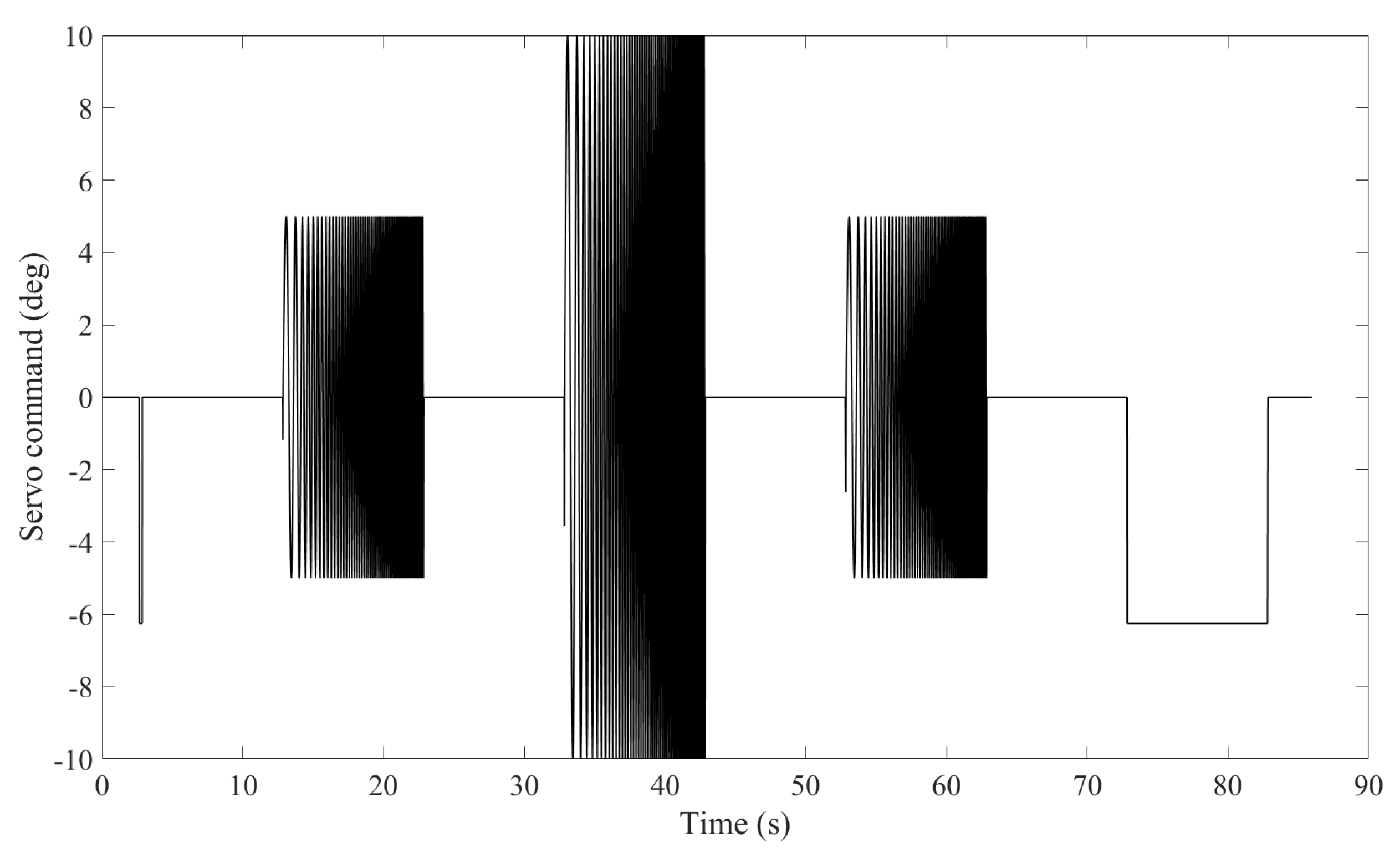
Figure 19.
CAD layout of the A3TB-WT with the root area highlighted in black (left) and the FEM representation of the PaPA mounting region and root spring (right).
Figure 19.
CAD layout of the A3TB-WT with the root area highlighted in black (left) and the FEM representation of the PaPA mounting region and root spring (right).
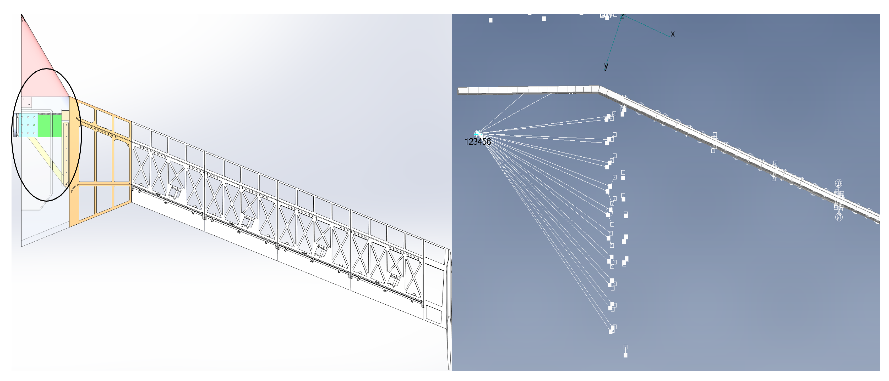
Figure 20.
FFT of the wind-tunnel GVT time history for configuration 1 recovered using FOS data.
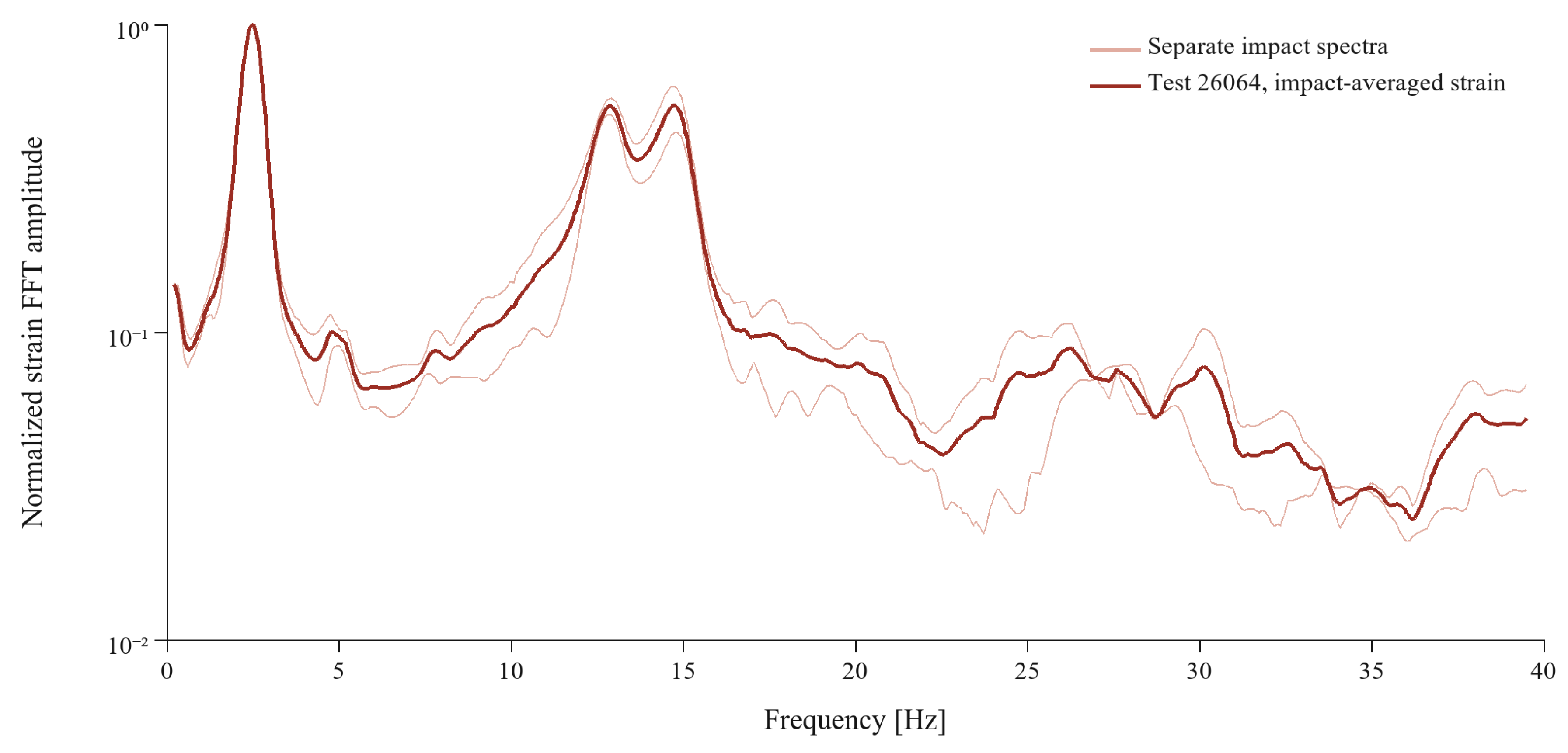
Figure 21.
Estimated aeroelastic frequencies, modal damping ratios, and stability parameter based on strain data.
Figure 21.
Estimated aeroelastic frequencies, modal damping ratios, and stability parameter based on strain data.
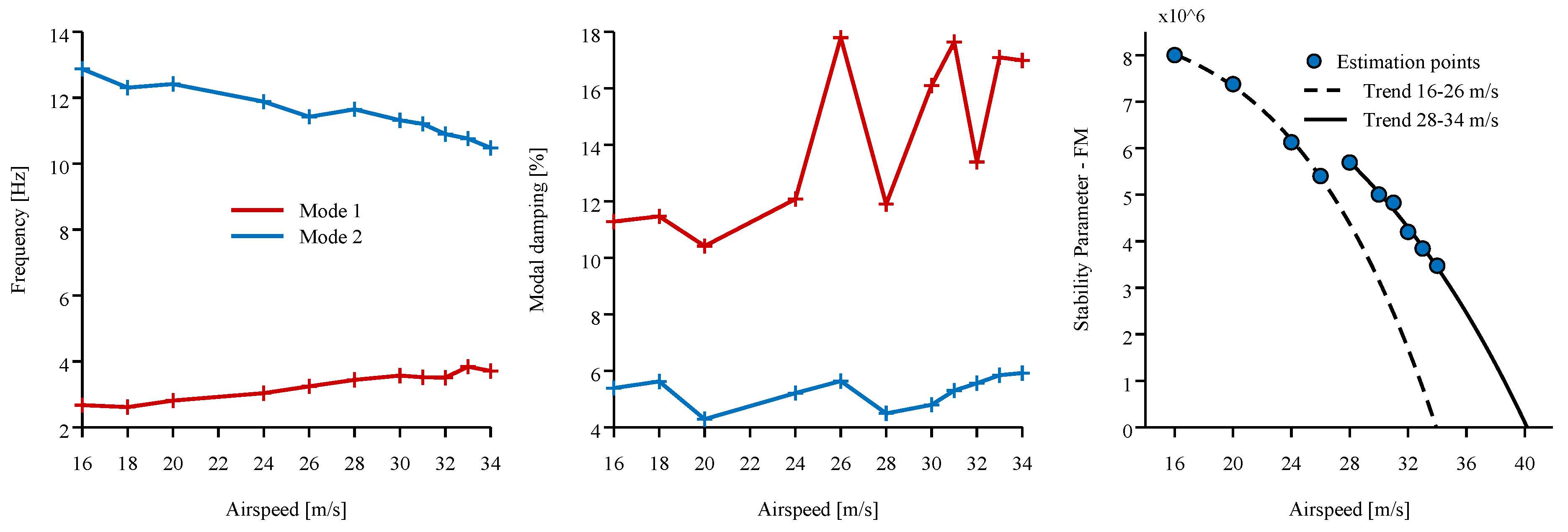
Figure 22.
Estimated aeroelastic frequencies, modal damping ratios, and flutter margin from the acceleration-based VARMA analysis.
Figure 22.
Estimated aeroelastic frequencies, modal damping ratios, and flutter margin from the acceleration-based VARMA analysis.
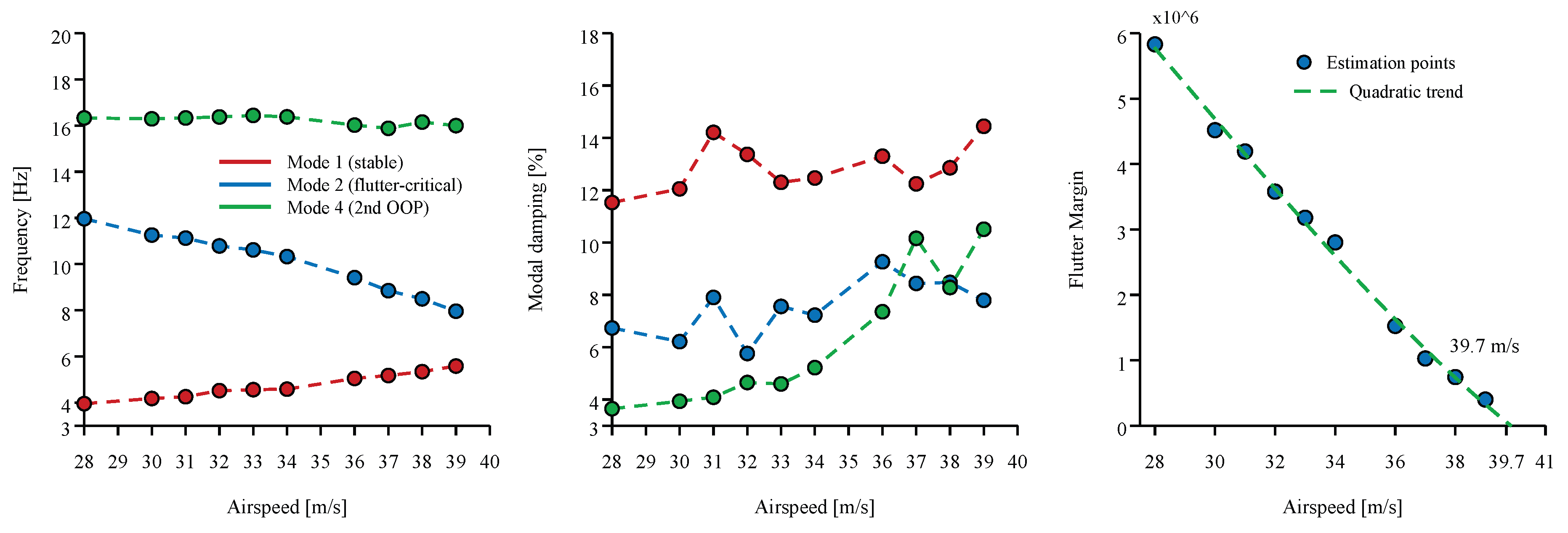
Figure 23.
Gain (top) and phase (bottom) of from test, –42 m/s. The nominal flutter condition is inferred from the unity-gain crossing at the phase-cross-over frequency.
Figure 23.
Gain (top) and phase (bottom) of from test, –42 m/s. The nominal flutter condition is inferred from the unity-gain crossing at the phase-cross-over frequency.
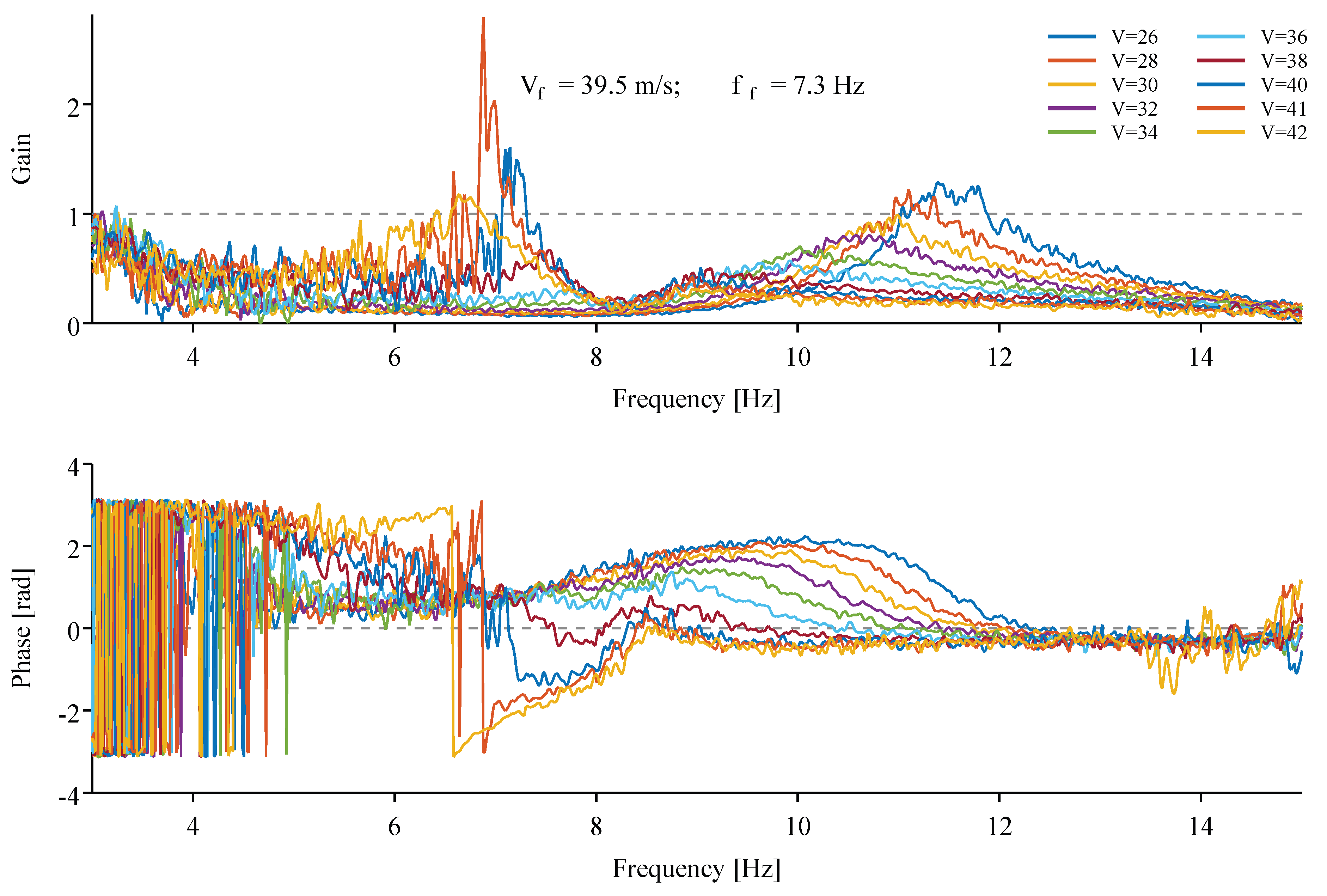
Figure 24.
Postprocessing data from the FOS and MCS during wind tunnel tests at 26 m/s. Three different test profiles with various control surface excitations reconstructed from the data are shown.
Figure 24.
Postprocessing data from the FOS and MCS during wind tunnel tests at 26 m/s. Three different test profiles with various control surface excitations reconstructed from the data are shown.
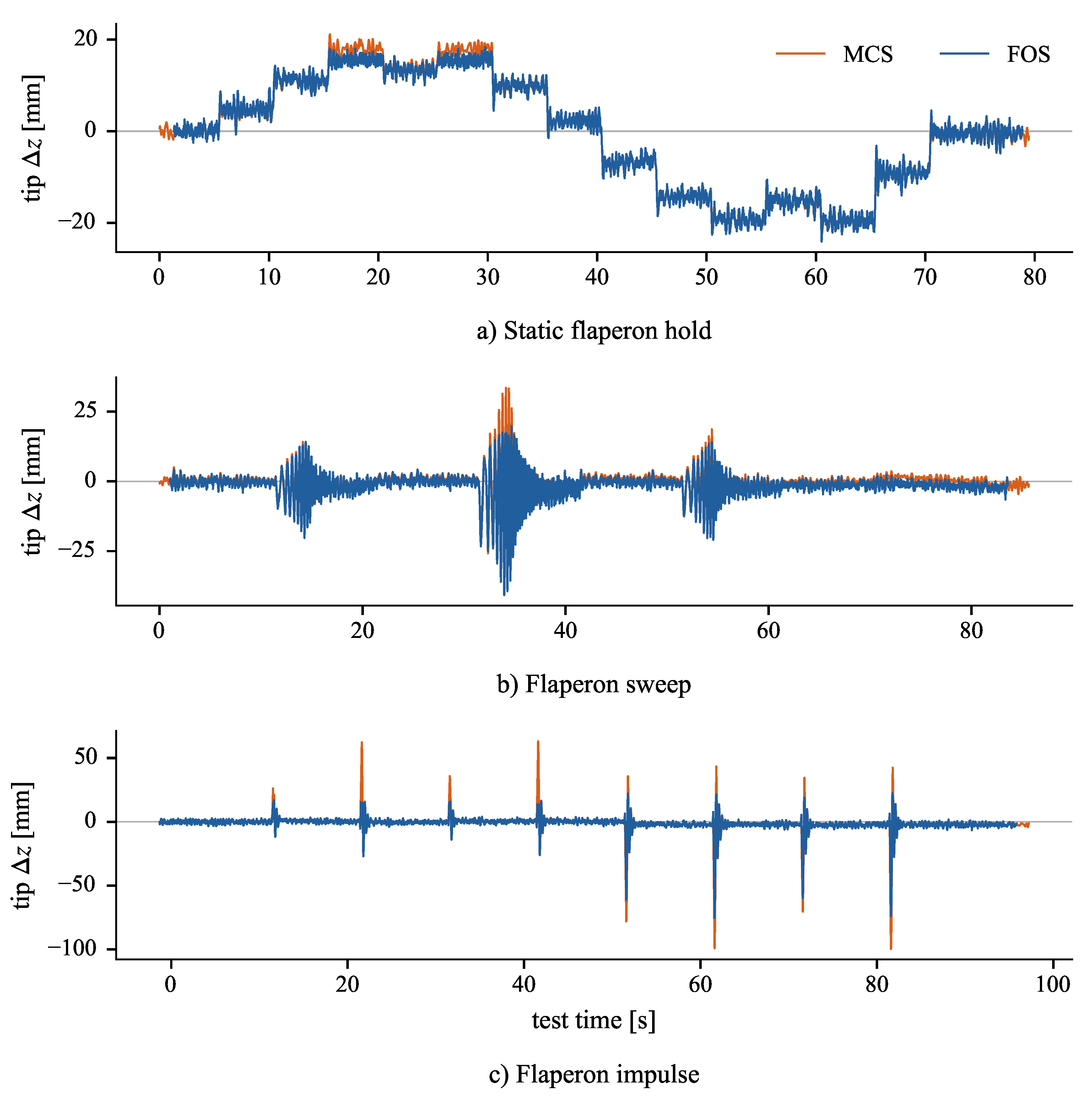
Figure 25.
Wing deformation recovered from FOS strain measurements during a 26 m/s static flaperon test in which the most outboard control surface followed a stepped deflection profile.
Figure 25.
Wing deformation recovered from FOS strain measurements during a 26 m/s static flaperon test in which the most outboard control surface followed a stepped deflection profile.
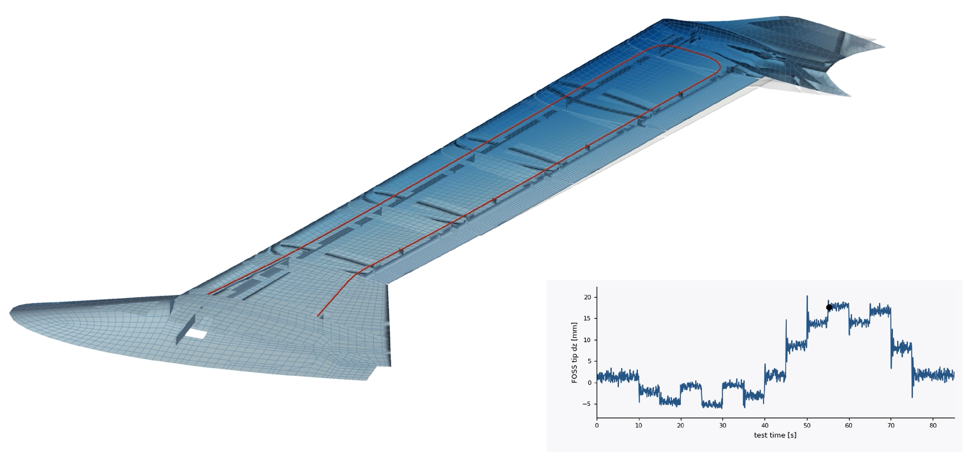
Figure 26.
Wing deformation recovered from MCS marker measurements during a 26 m/s static flaperon test in which the most outboard control surface followed a stepped deflection profile.
Figure 26.
Wing deformation recovered from MCS marker measurements during a 26 m/s static flaperon test in which the most outboard control surface followed a stepped deflection profile.
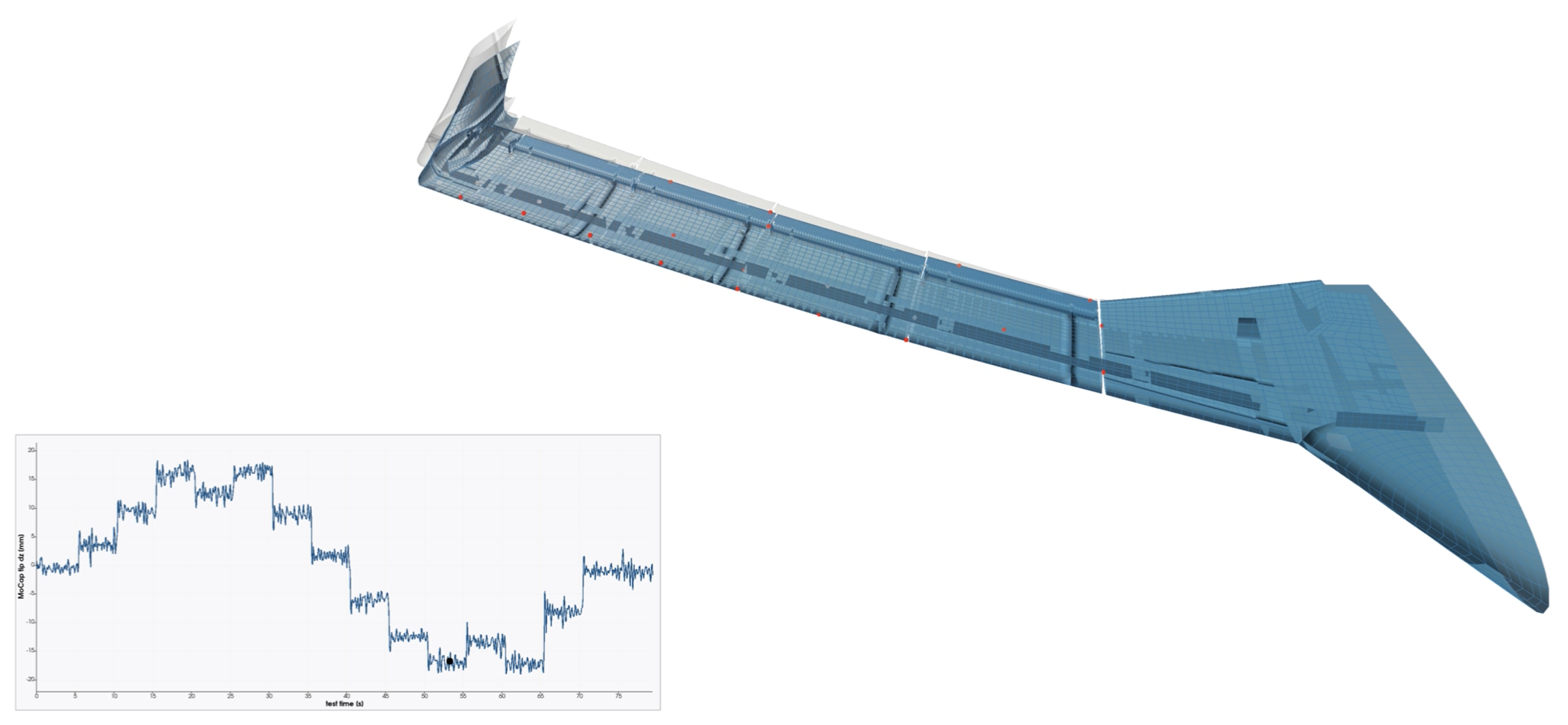
Table 1.
Reference A3TB model details.
| Item | Value | Units |
|---|---|---|
| Wingspan | 3 | m |
| Sweep angle | 22 | deg |
| Geometric pretwist at the tip | −3 | deg |
| Airfoil | NACA 0012 | N/A |
| Control surfaces | 8 trailing-edge flaperons | N/A |
| Main 3D printing material | PA-12 Nylon | N/A |
| Spar cross-section dimensions | 20 × 5 | mm × mm |
| Spar material | Woven carbon fiber | N/A |
Table 2.
Combined wind-tunnel test envelope for both configurations of the A3TB-WT.
| Variable term | Ranges | Increments | Unit | Type | |
|---|---|---|---|---|---|
| Configuration 1 | Root angle of attack | 3 or 5 | − | deg | Fixed by airspeed range |
| Airspeed | 16 to 39 | 1 or 2 | m/s | Fixed at each interval | |
| Flaperon | to +1 | 0.33 | Normalized | Static, individual and combined | |
| Flaperon | 1 to 10 | − | Hz | Sweep (10 s duration) | |
| Flaperon | to | Variable | Normalized | Impulse | |
| Variable term | Ranges | Increments | Unit | Type | |
| Configuration 2 | Root angle of attack | 3 or 5 | − | deg | Fixed by airspeed range |
| Airspeed | 20 to 42 | 1 or 2 | m/s | Fixed at each interval | |
| Flaperon | to | variable | Normalized | Impulse | |
| Tip shaker | 3 to 15 | − | Hz | Sweep | |
| Tip shaker | − | s | Impulse |
Table 3.
Summary of data collected during the A3TB-WT wind tunnel test (WTT) campaign.
| Type of test | Instrumentation | Type of data |
|---|---|---|
| GVT | Motion capture system | Marker displacement |
| Vibration accelerometers | Accelerations and frequency-response functions | |
| Fiber optic system | Strains along span | |
| WTT | Motion capture system | Marker displacement |
| Fiber optic system | Strains along span | |
| Accelerometers | Accelerations at wingtip | |
| Shaker board | Shaker and board accelerations | |
| Control surface commands | Normalized pulse-width-modulation signal | |
| PaPA rotary encoder | Root angle of attack | |
| PaPA load cell | Three forces and three moments |
Table 4.
Natural frequencies (Hz) for configuration 1 with and without skin and configuration 2 of the initial A3TB-WT finite element model. Modes labeled as OOP are out-of-plane bending, IP are in-plane bending, T are torsion, and CS are control surface modes.
Table 4.
Natural frequencies (Hz) for configuration 1 with and without skin and configuration 2 of the initial A3TB-WT finite element model. Modes labeled as OOP are out-of-plane bending, IP are in-plane bending, T are torsion, and CS are control surface modes.
| Configuration 1 | Configuration 2 | |||||
|---|---|---|---|---|---|---|
| Mode # | Skin-off | Mode type | Skin-on | Mode type | Skin-on | Mode type |
| 1 | 3.25 | 1 OOP | 3.29 | 1 OOP | 2.96 | 1 OOP |
| 2 | 10.09 | 1 T | 11.02 | 1 T | 9.54 | 1 T |
| 3 | 12.38 | 1 IP | 13.76 | 1 IP | 12.22 | 1 IP |
| 4 | 17.05 | 2 OOP | 17.76 | 2 OOP | 17.62 | 2 OOP |
| 5 | 27.57 | Wingtip | 31.48 | 3 OOP | 31.13 | 3 OOP |
| 6 | 30.55 | 3 OOP/CS | 35.17 | T 2/CS | 33.97 | T 2/CS |
| 7 | 34.30 | T 2/CS | 36.28 | T 2/CS | 36.15 | T 2/CS |
| 8 | 35.01 | CS | 37.28 | T 2/CS | 37.17 | CS |
| 9 | 36.25 | CS | 50.40 | CS | 50.53 | CS |
| 10 | 44.89 | 2 IP | 52.21 | CS | 51.50 | CS |
| 11 | 49.12 | CS | 52.89 | 2 IP | 52.53 | 2 IP |
Table 5.
GVT results (frequencies in Hz) using the vibration accelerometers for configuration 1 with and without skin.
Table 5.
GVT results (frequencies in Hz) using the vibration accelerometers for configuration 1 with and without skin.
| Configuration 1 without skin | Configuration 1 with skin | |||||||
|---|---|---|---|---|---|---|---|---|
| Impact Hammer | Shaker | Impact Hammer | Shaker | |||||
| Mode # | Frequency | Mode type | Frequency | Mode type | Frequency | Mode type | Frequency | Mode type |
| 1 | 2.46 | 1 OOP | 2.47 | 1 OOP | 2.48 | 1 OOP | 2.49 | 1 OOP |
| 2 | – | 1 IP | 6.78 | Unknown | – | 1 IP | 7.15 | 1 IP |
| 3 | 11.40 | 1 T | 11.44 | 1 T | 12.10 | 1 T | 11.78 | 1 T |
| 4 | 13.20 | 2 OOP | 13.18 | 2 OOP | 14.70 | 2 OOP | 14.83 | 2 OOP |
| 5 | 25.20 | 3 OOP | 25.44 | 3 OOP | 33.7 | 3 OOP | 33.03 | 3 OOP |
Table 6.
GVT results (frequencies in Hz) using the vibration accelerometers for configuration 2 with skin.
Table 6.
GVT results (frequencies in Hz) using the vibration accelerometers for configuration 2 with skin.
| Impact Hammer | Shaker | |||
|---|---|---|---|---|
| Mode # | Frequency | Mode type | Frequency | Mode type |
| 1 | 2.3 | 1 OOP | 2.32 | 1 OOP |
| 2 | – | 1 IP | 6.78 | 1 IP |
| 3 | 11.86 | 1 T/ 2 OOP | 11.81 | 1 T |
| 4 | 12.98 | 1 IP/1T | 12.64 | 2 OOP |
| 5 | 26.72 | 3 OOP | 26.52 | 3 OOP |
Table 7.
Comparison of natural frequencies (Hz) between the initial configuration 1 with-skin FEM and the as-built structure outside the wind tunnel.
Table 7.
Comparison of natural frequencies (Hz) between the initial configuration 1 with-skin FEM and the as-built structure outside the wind tunnel.
| Mode # | FEM | Mode type | GVT | Mode type | % Error |
|---|---|---|---|---|---|
| 1 | 3.29 | 1 OOP | 2.49 | 1 OOP | 32.1% |
| 2 | 13.76 | 1 IP | 7.15 | 1 IP | 92.4% |
| 3 | 11.02 | 1 T | 11.78 | 1 T | −6.5% |
| 4 | 17.76 | 2 OOP | 14.83 | 2 OOP | 19.8% |
| 5 | 31.48 | 3 OOP | 33.03 | 3 OOP | −4.7% |
Table 8.
Comparison of natural frequencies (Hz) for configuration 1 with skin between the different experimental systems used for GVT conducted under laboratory conditions. MCS and FOS results are from the impact hammer excitation only.
Table 8.
Comparison of natural frequencies (Hz) for configuration 1 with skin between the different experimental systems used for GVT conducted under laboratory conditions. MCS and FOS results are from the impact hammer excitation only.
| Mode # | MCS Impact | FOS Impact | Accel. Impact | Accel. Shaker | Mode type |
|---|---|---|---|---|---|
| 1 | 2.6 | 2.6 | 2.48 | 2.49 | 1 OOP |
| 2 | 7.1 | 6.9 | – | 7.15 | 1 IP |
| 3 | 12.1 | 11.9 | 12.1 | 11.8 | 1 T |
| 4 | 15.0 | 15.1 | 14.7 | 14.8 | 2 OOP |
| 5 | – | – | 33.7 | 33.03 | 3 OOP |
Table 9.
Comparison of the physically corrected FEM with GVT for configuration 1 without skin.
| Type | MCS | FOS | LMS Impact | LMS Shaker | FEM |
|---|---|---|---|---|---|
| 1 OOP | 2.3 | 2.5 | 2.5 | 2.5 | 2.4 |
| 1 T | 11.3 | 11.4 | 11.4 | 11.4 | 10.1 |
| 1 T/1 IP | – | 6.8 | – | – | 11.7 |
| 2 OOP | 13.1 | 13.4 | 13.2 | 13.2 | 15.1 |
Table 10.
Comparison of the physically corrected FEM with GVT for configuration 1 with skin.
| Type | MCS | FOS | LMS Impact | LMS Shaker | FEM |
|---|---|---|---|---|---|
| 1 OOP | 2.6 | 2.6 | 2.5 | 2.5 | 2.6 |
| 1 IP | 7.1 | 6.9 | – | 7.1 | 13.4 |
| 1 T | 12.1 | 11.9 | 12.1 | 11.8 | 11.1 |
| 2 OOP | 15.0 | 15.1 | 14.7 | 14.8 | 15.9 |
Table 11.
Design variables for the FEM updating using shaker table GVT results.
| Variable type | Component | Normalized bounds | Initial value | Final value | Units | Difference (vs. initial) % |
|---|---|---|---|---|---|---|
| Density | 3D printed | 0.95, 1.05 | 890.00 | 889.11 | 0.1 | |
| Density | Composite spar | 0.95, 1.05 | 1471.50 | 1465.61 | 0.4 | |
| Density | Fin | 0.95, 1.05 | 824.41 | 788.96 | 4.3 | |
| Density | Fuselage | 0.95, 1.05 | 950.00 | 950.48 | 0.1 | |
| Young’s Modulus | 3D printed | 0.75, 1.25 | 1.80 | 1.36 | GPa | 24.5 |
| Young’s Modulus | skin | 0.5, 5.0 | 1.83 | 5.84 | GPa | 220. |
| or | Composite spar | 0.8, 1.2 | 45.00 | 54.00 | GPa | 20.0 |
| Composite spar | 0.8, 1.2 | 2.01 | 2.07 | GPa | 2.8 | |
| Young’s Modulus | Fuselage | 0.75, 1.25 | 1.65 | 1.49 | GPa | 10.0 |
| Root spring | 0.75, 1.5 | 0.0 | ||||
| Root spring | 0.75, 1.5 | 0.0 | ||||
| Root spring | 0.75, 1.5 | 0.0 | ||||
| Root spring | 0.75, 2.0 | 100.0 | ||||
| Root spring | 0.75, 1.5 | 0.0 | ||||
| Root spring | 0.75, 1.5 | 41.0 |
Table 12.
Results from the FEM calibration using the shaker table GVT data for configuration 1.
| GVT on shaker base | Physically corrected FEM | Laboratory-calibrated FEM | ||||
|---|---|---|---|---|---|---|
| Mode # | Mode type | Frequency [Hz] | Frequency [Hz] | Difference (vs. GVT) % | Frequency [Hz] | Difference (vs. GVT) % |
| 1 | 1 OOP | 2.49 | 2.21 | −11.4 | 2.50 | 0.5 |
| 2 | 1 IP | 7.15 | 6.31 | −11.7 | 7.15 | 0.0 |
| 3 | 1 T | 11.78 | 10.58 | −10.2 | 11.79 | 0.1 |
| 4 | 2 OOP | 14.83 | 13.04 | −12.1 | 14.55 | −1.9 |
| 5 | 3 OOP | 33.03 | 30.68 | −7.1 | 33.37 | 1.0 |
Table 13.
Comparison of natural frequencies (Hz) for GVT performed in the wind tunnel. MCS and FOS results are from wind-off testing with the model mounted on the wind tunnel apparatus.
Table 13.
Comparison of natural frequencies (Hz) for GVT performed in the wind tunnel. MCS and FOS results are from wind-off testing with the model mounted on the wind tunnel apparatus.
| Mode # | MCS | FOS | FEM | Mode type |
|---|---|---|---|---|
| 1 | 2.6 | 2.5 | 2.50 | 1 OOP |
| 2 | 7.1 | 7.1 | 7.15 | 1 IP |
| 3 | 11.9 | 12.0 | 11.79 | 1 T |
| 4 | 15.3 | 15.1 | 14.55 | 2 OOP |
| 5 | – | 35.5 | 33.37 | 3 OOP |
Table 14.
Design variables for the FEM updating using wind tunnel GVT results.
| Variable type | Component | Normalized bounds | Initial value | Final value | Units | Difference (vs. initial) % |
|---|---|---|---|---|---|---|
| Root spring | 0.75, 1.5 | 0.0 | ||||
| Root spring | 0.75, 1.5 | 0.0 | ||||
| Root spring | 0.75, 1.5 | 0.0 | ||||
| Root spring | 0.75, 2.0 | 54.1 | ||||
| Root spring | 0.75, 1.5 | 0.0 | ||||
| Root spring | 0.75, 1.5 | 2.0 |
Table 15.
Results from the wind tunnel FEM calibration for configuration 1.
| GVT in wind tunnel | Laboratory-calibrated FEM | Mounted calibrated FEM | ||||
|---|---|---|---|---|---|---|
| Mode # | Mode type | Frequency [Hz] | Frequency [Hz] | Difference (vs. GVT) % | Frequency [Hz] | Difference (vs. GVT) % |
| 1 | 1 OOP | 2.6 | 2.50 | −4.5 | 2.62 | −0.1 |
| 2 | 1 IP | 7.1 | 7.15 | 0.7 | 7.12 | 0.2 |
| 3 | 1 T | 12.0 | 11.79 | −1.7 | 11.89 | −0.9 |
| 4 | 2 OOP | 15.1 | 14.55 | −3.7 | 15.23 | 0.9 |
| 5 | 3 OOP | 35.5 | 33.37 | −6.0 | 35.13 | −1.0 |
Disclaimer/Publisher’s Note: The statements, opinions and data contained in all publications are solely those of the individual author(s) and contributor(s) and not of MDPI and/or the editor(s). MDPI and/or the editor(s) disclaim responsibility for any injury to people or property resulting from any ideas, methods, instructions or products referred to in the content. |
© 2026 by the authors. Licensee MDPI, Basel, Switzerland. This article is an open access article distributed under the terms and conditions of the Creative Commons Attribution (CC BY) license (http://creativecommons.org/licenses/by/4.0/).
Copyright: This open access article is published under a Creative Commons CC BY 4.0 license, which permit the free download, distribution, and reuse, provided that the author and preprint are cited in any reuse.


