

Submitted:
31 July 2026
Posted:
03 August 2026
You are already at the latest version
Abstract
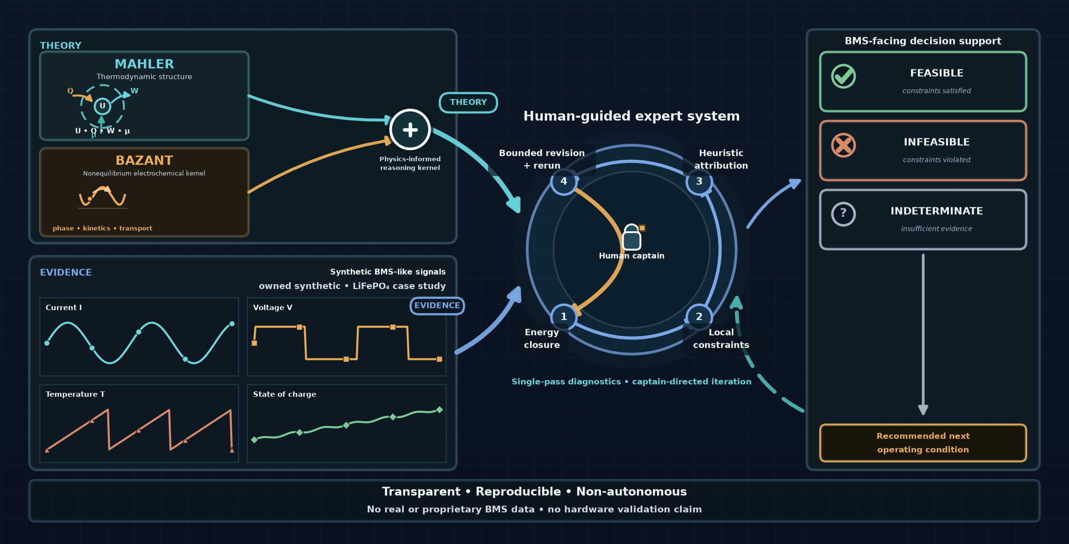
This methodological case study demonstrates how a human-guided AI expert system applies heuristic reasoning to synthetic signals representative of those from an onboard battery-management system, using the LiFePO₄ single-particle electrochemical model as an analytical test bed. The work is conducted as a structured dialogue between a human domain expert and an AI expert system. The framework grounds the bivariate kernel V = μ + W — equilibrium chemical potential μ plus non-equilibrium reaction work W — in the Mahler bivariate first law of nonequilibrium thermodynamics, exploits the regular-solution symmetry of LiFePO₄ at c = 1/2 to identify W as a directly observable thermodynamic field, and develops a reference logic and three-stage attribution heuristic discriminating concentration-polarization memory, phase morphology change, and thermal feedback contributions to the measured W under GITT protocol. A lumped enthalpy balance runs alongside as a local thermal-constraint instrument on the convective heat-transfer coefficient, returning a per-iteration constraint margin and flag rather than a terminal verdict; the joint report combines the mechanism attribution with the local thermal-constraint flag as two independent, non-terminal diagnostic signals. An integral solver/model energy-closure check gates each candidate simulation for admissibility before the thermal-constraint and iterative-feasibility stages, so only energetically consistent candidates are interpreted.
Keywords:
AI-assisted reasoning
; nonequilibrium thermodynamics
; LiFePO4
; single-particle model
; Mahler
; symmetry-point identity
; local thermal-constraint instrument
1. Introduction
1.1. The Artifact and the Claim
This paper presents a case study in AI-assisted heuristic reasoning, conducted as a dialogue between a human domain expert and a large language model acting as an expert system. The dialogue constructs a falsifiable framework for extending the single-particle lithium iron phosphate (LFP) electrochemical model into operating regimes where its standard derivation breaks down. The artifact produced — a reference logic that calibrates a bare Butler–Volmer kernel at the regular-solution symmetry point and tests, through a controlled deviation metric, whether the coupled exchange-current term of the Cahn–Hilliard reaction theory of Zeng and Bazant [1] is statistically distinguishable from measurement noise in a given dataset — is documented in Section 4. The artifact is not, however, the principal contribution.
The principal contribution is the methodological framework under which the artifact was constructed. The work claims that AI-assisted heuristic reasoning, when properly disciplined, can extend a partially closed physical theory into a region where neither pure first-principles derivation nor pure data fitting is adequate, and that the required discipline is identifiable, describable, and reproducible. The LFP single-particle model serves as the diagnostic test bed: its closed regime is rigorously derived [1,2], its breakdown modes are diagnosable through specific symmetry and scaling tests, and its constitutive structure admits a clean partition between equilibrium thermodynamic and kinetic content. These features let the dialogue’s structural moves be checked against well-posed mathematical objects rather than intuition, and each provides a falsifiability anchor that distinguishes disciplined extension from speculation.
The framework’s contribution is therefore not a new electrochemical model. It is a documented protocol — and an account of how that protocol was generated — for the heuristic extension of partially closed physical theories where the canonical derivation does not reach the operating regime of interest. The LFP application demonstrates that the protocol converges to a falsifiable artifact within a finite number of exchanges; the protocol itself is what is offered as transferable.
Many engineering inference problems are neither model-free nor fully closed. Conservation relations and qualitative physical structure restrict admissible behavior, but uncertain parameters, unmodeled mechanisms, and limited observability may prevent a unique inverse conclusion [3]. Qualitative simulation therefore represents behavior as a set of physically possible trajectories [4], while consistency-based diagnosis generates and revises candidate explanations as additional evidence becomes available [5]. The present framework extends this lineage by placing transparent heuristic attribution between a physical admissibility gate and a human-directed bounded-rerun process, with indeterminate retained as a legitimate outcome rather than treated as a failed classification.
1.2. Roles and Responsibilities in the Dialogue
A central methodological commitment of this work is the explicit, asymmetric partition of responsibility between the human captain and the AI expert system. The two roles are not interchangeable and the dialogue’s convergence depends on each being executed within its proper scope.
The AI expert system functions in two capacities. First, as a generator of structural candidates: it proposes decompositions, identifies functional forms compatible with the imposed constraints, retrieves and verifies canonical equations of the domain literature, and generates hypotheses against which the captain’s domain knowledge is brought to bear. Second, as a checker of dimensional and structural consistency: it tests whether proposed kernels satisfy required symmetries (charge-discharge invariance, asymptotic limits, dimensional homogeneity), whether asymptotic behaviors are mutually compatible, and whether the partition of a measured signal among postulated contributions is unique under the stated assumptions. The AI is thus a tireless generator-checker whose value lies in maintaining structural discipline across an extended sequence of moves, not in supplying domain-specific scientific judgment.
The human captain holds three responsibilities the AI cannot discharge. First, domain-specific scoping: which physical questions are well-posed, which observables are accessible, which canonical limits must be respected, and which simplifications are admissible without abandoning the phenomenon. Second, corrective filtering: identifying AI proposals that are structurally permissible but physically inappropriate, rejecting digressions from the load-bearing question, and retracting prior commitments when new considerations invalidate them. Third, final structural selection: the authoritative choice among AI-generated candidates of kernel components, reference states, symmetry anchors, and diagnostic metrics. The captain’s authority is not advisory and AI proposals are not adopted by default; selection is an explicit act for which the captain is responsible.
The asymmetry is essential. The AI generates more candidates than are correct, and correctness cannot be settled by structural checking alone; the captain’s filtering is therefore the load-bearing operation guarding against plausibly-structured but physically vacuous models. Conversely, the captain’s intuition is no substitute for the AI’s sustained structural bookkeeping — dimensional consistency, asymptotic compatibility, and partition uniqueness tracked across many exchanges — which guards against physically motivated but structurally incoherent models. Each role guards against a failure the other cannot detect. This governance posture — an AI reasoning layer whose symbolic proposals are validated and corrected by a human expert to control hallucination — has a direct precedent in the use of large language models to draft expert-system knowledge that domain experts then verify [6].
1.3. The Diagnostic Value of the LFP Test Bed
The single-particle LFP model is not an arbitrary test bed. It is selected for three properties that make AI-assisted heuristic extension diagnostically informative rather than merely demonstrative.
First, the model possesses an exact symmetry point: the regular-solution chemical potential vanishes identically at half-lithiation under the homogeneous, uniform-composition derivation, providing a calibration anchor at which the equilibrium and kinetic voltage contributions are structurally separable without fitting. This anchor is what permits Section 4’s deviation metric to be a falsifiable test rather than a model-selection criterion.
Second, the model has a well-characterized derivation envelope. The Cahn–Hilliard reaction theory of Bazant [2] and the spherical-particle treatment of Zeng and Bazant [1] are derived under explicit assumptions — uniform composition, symmetric Butler–Volmer kinetics, regular-solution thermodynamics with a single interaction parameter, single-particle isolation from population effects — each identifiable, independently testable, and known to fail in a specific regime. Captain domain expertise can therefore locate the envelope boundary unambiguously, and AI structural checking can test whether a proposed extension respects the boundary it claims to cross.
Third, the model’s known limitations are themselves quantitative: uniform-composition breakdown at finite current is characterized by the diffusion-limited current and the current at which phase separation is dynamically suppressed; single-particle-isolation breakdown by population integrals whose moments depend on cell architecture; isothermal breakdown by the Arrhenius temperature coupling of the exchange current.
Together — exact symmetry, a well-bounded derivation envelope, and quantified limitations — these render the LFP single-particle model a diagnostic instrument rather than a target application. The framework’s success or failure here is informative about the framework itself in a way a less rigorously characterized system would not be; the paper’s claim is about the framework’s structure and discipline, with the LFP outcome as evidence that it can converge on a falsifiable artifact within the dialogue’s resource constraints.
The remainder of the paper documents the dialogue process (Section 2), the implications for AI-assisted reasoning in partially closed physical theories (Section 3), the reference logic (Section 4), the attribution metrics by which the artifact may be tested against experimental data (Section 5), the illustrative worked example (Section 6), and the discussion of related modeling approaches and transfer limits (Section 7).
This methodological case study demonstrates how a human-guided AI expert system applies heuristic reasoning to synthetic signals representative of those available from an onboard battery-management system. The signals are synthetic by design: current, voltage, temperature, state of charge, pulse and rest timing, and the derived reaction-work residual channel are produced by a fully owned, deterministic Python generator with fixed configurations and seeds and declared physics-informed constraints (an analytical open-circuit-voltage form, a lumped thermal balance, and a cited entropic term). They are controlled perturbations on a known baseline, not proprietary or inaccessible measurements, and the study evaluates the reasoning’s transparency, consistency, traceability, falsifiability, and recognition of insufficient evidence rather than empirical accuracy. Using physically grounded synthetic signals to exercise battery-management algorithms is established practice — for example, virtual battery packs built from equivalent-circuit and lumped-thermal models [7] — and grounding a diagnostic method on simulation-generated signals, with explicit validation of the synthetic stream as a named pipeline step, is standard in simulation-based diagnosis [8].
1.4. The Symmetry-Point Identity and Its Derivational Grounding
The bivariate kernel V = μ + W introduced in §1.1 is not posited by this framework. It is the electrochemical instance of a nonequilibrium bivariate first law derived by Gemmer, Michel, and Mahler in Quantum Thermodynamics §4.3 [9]. The present section establishes the derivation chain, identifies the framework’s interpretive choices, and develops the symmetry-point identity on which the reference logic of Section 4 and the attribution heuristics of Section 5 depend.
1.4.1. Mahler’s Bivariate First Law
Mahler establishes the bivariate first law for a single thermodynamic system through Eqs. (4.75)–(4.86) of his §4.3. The internal energy of a system characterized by two control parameters α and γ admits the differential decomposition
The first term, after manipulation through the von Neumann entropy, becomes the heat contribution (Definition 4.14):
The second term is identified as work (Definition 4.16):
The first law follows (Eq. 4.86):
The structural content of these equations is that internal energy admits a bivariate decomposition into a heat contribution coupled to entropy change and a work contribution coupled to change in a non-thermal control parameter. The two terms are independent: one varies α at fixed γ, the other varies γ at fixed α.
Mahler then generalizes the non-thermal control parameter in Definition 4.23, Eq. (4.91), with the explicit qualifier “where Z2 need not even be mechanical in the strict sense.” This generalization is load-bearing: it authorizes the non-thermal control axis to be any parameter whose conjugate variable is intensive. The instances Mahler enumerates on p. 200 include volume against pressure (d_V U = -p dV), polarization against electric field (d_P U = E · dP), magnetization against magnetic field (d_M U = B · dM), and — most relevantly for the present framework — particle number against chemical potential (Definition 4.24):
The Gibbs fundamental form (Definition 4.25, Eq. 4.102) collects the contributions in differential form:
with T, ξ2, ξ3, … the intensive conjugates of the extensive control parameters S, Z2, Z3, …. The framework adopts this as the structural form for the bivariate kernel.
1.4.2. The Classical Limit and Its Applicability to the LFP Single Particle
Mahler’s derivation is conducted within the quantum-thermodynamic formalism, but the framework’s domain of application is the classical or quasi-classical LFP particle. Mahler addresses the validity of the classical limit explicitly in Definition 4.12, Eq. (4.74):
with λ_dB the thermal de Broglie wavelength and R the average inter-particle distance. The accompanying text states: “For a single particle R is infinite.” Mahler thus establishes that the classical limit holds by construction for the single-particle case — τ → 0 trivially as R → ∞. The framework inherits this conclusion: the LFP single-particle case is the natural domain of application of Mahler’s derivation chain, not an extension of it.
One minor refinement is acknowledged. The LFP particle is a composite object — a host lattice containing many lithium atoms — rather than a point particle. The classical limit applies to the particle as a thermodynamic system with internal degrees of freedom (composition c, electronic state), because the particle itself is macroscopic relative to any thermal de Broglie wavelength of the relevant degrees of freedom. The applicability of Mahler’s framework to LFP is therefore direct and does not require an interpretive bridge between quantum and classical regimes.
1.4.3. The Framework’s Interpretive Identification
Mahler’s framework authorizes the bivariate first-law structure but does not specify which physical control parameter is identified with the generalized non-thermal axis Z2 in any particular application. The framework adopts the following identification for the LFP single-particle electrochemical system:
- The chemical control axis is identified with lithium insertion, with Z3 = N_Li the extensive particle number and ξ3 = μ the chemical potential of lithium in the particle. This identification follows Mahler’s Definition 4.24 directly and requires no interpretive step.
- The generalized work axis is identified with the driving extent — the integrated charge passed through the cell, normalized appropriately — with ξ2 ≡ -ξ_W the non-equilibrium reaction-work density per unit driven extent. This identification is the framework’s interpretive choice. Mahler’s Definition 4.23 authorizes the non-thermal axis to be non-mechanical, but does not establish the specific identification of Z2 with a driven electrochemical extent. The framework adopts this identification as its primary structural commitment and acknowledges it as an interpretive move beyond what Mahler explicitly derives. The legitimacy of the identification rests on its empirical validation through the symmetry-point identity (§1.4.4) and through the discrimination heuristics of Section 5, not on Mahler’s derivation alone.
Under these identifications, the cell voltage V is related to the internal energy contributions per unit lithium insertion via
where the factor of e absorbs the conversion between energy per Li atom and voltage, and V^Θ is the reference potential fixed by the convention μ_eq(c = 1/2) = 0. The bivariate kernel V = μ + W of §1.1 is, in this presentation, the absorbed-unit form of this Mahler-derived relation.
1.4.4. The Symmetry-Point Identity
The framework’s central structural result follows from Mahler’s bivariate first law applied at the regular-solution symmetry point of the LFP chemical potential. The regular-solution form
(see Ref. [2] for the derivation in the electrochemical context) vanishes identically at c̃ = 1/2. The vanishing is structural: both the entropic and enthalpic contributions are zero by symmetry of the homogeneous free energy, independent of Ω̃ or temperature.
At the symmetry point, the chemical-control contribution μ dN to the Mahler decomposition vanishes, and the cell voltage offset from the reference potential reduces to the work contribution alone:
This is the symmetry-point identity. It is the only point on the discharge curve where the bivariate kernel’s two fields decouple by construction, and it is the framework’s load-bearing observable.
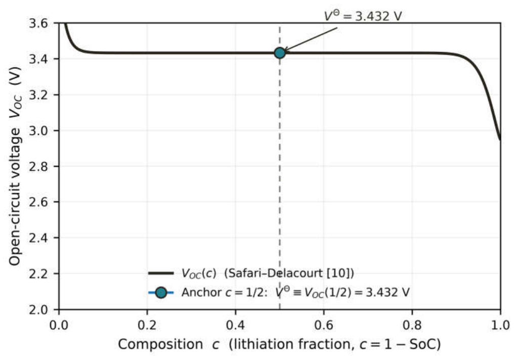
Line plot of the elected Safari-Delacourt LiFePO4 open-circuit voltage curve versus lithium composition, showing the characteristic flat plateau near 3.43 volts. A dashed vertical line at the composition midpoint marks the anchor, where the reference potential equals the open-circuit voltage read at that point, 3.432 volts.
Figure 1.
Elected open-circuit voltage curve (Safari & Delacourt [10] analytical LFP form) with the anchor point at marked. Under the paper’s convention (§4), the standard potential is defined by the symmetry constraint , which places at the value of the elected OCV curve read at the anchor composition: V for the Safari–Delacourt election. The election is of the whole curve; the anchor scalar is where the framework’s symmetry-point identity is read. Analytical/synthetic supporting illustration (generated from the declared OCV model), not measured data.
Figure 1.
Elected open-circuit voltage curve (Safari & Delacourt [10] analytical LFP form) with the anchor point at marked. Under the paper’s convention (§4), the standard potential is defined by the symmetry constraint , which places at the value of the elected OCV curve read at the anchor composition: V for the Safari–Delacourt election. The election is of the whole curve; the anchor scalar is where the framework’s symmetry-point identity is read. Analytical/synthetic supporting illustration (generated from the declared OCV model), not measured data.
The identity has three immediate consequences.
First, the symmetry point provides direct measurement of the Mahler work contribution W at the LFP particle scale. No model of μ(c) and no low-current quasi-equilibrium extrapolation is required to read W at c = 1/2. The framework’s reference logic (Section 4) and attribution heuristics (Section 5) all operate on this directly measured quantity.
Second, the cell-level analog of the identity holds under the symmetry of the particle composition distribution. At the cell level, the measured voltage at average composition c̄ = 1/2 is the population average of single-particle voltages over the distribution of compositions in the cell. If the composition distribution is approximately symmetric around c = 1/2 — which holds, to working approximation, in homogeneously cycled LFP cells away from the mosaic-intercalation regime — the population average of μ(c) is approximately zero by the same symmetry that gives μ(1/2) = 0 at the particle level. The cell voltage at average SOC = 1/2 is therefore a population-averaged measurement of W at the cell scale.
Third, the symmetry-point identity is the bridge from the Mahler bivariate first law to the cell-level observable. The Mahler derivation establishes the structural form; the regular-solution symmetry of LFP provides the operational reduction; the population symmetry of the cell extends the identity to the macroscopic measurement. The three together make W at the symmetry point a directly observable thermodynamic field at both the single-particle and the cell scales.
1.4.5. The Role of Bazant–Zeng Kinetics in the Framework
The Mahler grounding establishes the structural content of the bivariate kernel. The framework also requires a kinetic content — a prediction for how W(1/2, I, t) depends on the driving current under specified assumptions — and this content is inherited not from Mahler but from the Bazant–Zeng kinetic kernel [1] (Eq. 4.1) verified by direct retrieval during the framework’s development:
Bazant–Zeng’s kernel provides the functional form W^BV(1/2, I) = (2k_BT/e)·sinh−1(I/2I0*) that Section 4’s reference logic tests as the bare Butler–Volmer null hypothesis H0 at the symmetry point. The Zeng–Bazant coupling (1-c)·exp(αμ̃) provides the structural prediction H1 tested against deviations from the bare form.
Bazant–Zeng kinetics serve two roles in the framework. As inspiration, they motivate the framework’s focus on the symmetry point: their derivation of Eq. (4.1) under the uniform-composition assumption clarified that the symmetry point is the location where the kernel’s content is operationally accessible, and this clarification motivated the framework’s structural exploitation of c = 1/2. As validation target, they provide the falsifiable kinetic prediction against which the directly measured W(1/2, I, t) is tested. The framework does not depend on Bazant–Zeng for its derivational structure — that is Mahler’s contribution — but it does depend on Bazant–Zeng for the specific kinetic prediction that makes the reference logic of Section 4 falsifiable.
1.4.6. Summary of the Framework’s Structural Grounding
The framework rests on a four-layer grounding:
- Mahler bivariate first law (Eqs. 4.85, 4.91, 4.97, 4.102; Definitions 4.16, 4.23, 4.24; classical limit established by Eq. 4.74) — derivational structure for the bivariate kernel V = μ + W.
- Regular-solution chemical potential [2] — operational reduction at the symmetry point where μ(1/2) = 0 and the bivariate kernel decouples.
- Cell-level lumped enthalpy balance as a local thermal-constraint instrument (Eq. (13) of §1.4.7; following Painter et al. [11] ) — lumped-thermal instrument whose role is not to reconstruct cell temperature dot-by-dot but to certify that convective cooling is sufficient to hold the cell near its ambient setpoint throughout the pulse-and-rest protocol. Under sufficient , the voltage-side symmetry-point observables (rest voltage) and (symmetry-point value) that the framework depends on are recoverable within the lumped model’s stated limitations. Under insufficient , the framework flags the operating condition as outside the local thermal-constraint band and invokes a three-metric failure-mode diagnostic (mean deviation, RMS deviation, and residual–current correlation over a rolling window) as a failure-mode identifier rather than a routine tracking measurement; §5.4 reports the local thermal-constraint status alongside every attribution result.
The framework’s interpretive contributions are three: the identification of the Mahler generalized work axis Z2 with the driven electrochemical extent (§1.4.3); the identification of W as per-charge reaction-work field at the symmetry point (§1.4.4); and the treatment of the enthalpy balance as a local thermal-constraint instrument rather than as a fitted or
shape-matched thermal model (§1.4.7). All four grounding layers are operational
rather than derivational: Mahler grounds the bivariate structure but does not
partition heat and work at the reaction step; regular-solution symmetry reduces
the kernel at c = 1/2 but does not derive the reaction rate; Bazant–Zeng gives
the bare-BV kinetic form but does not derive the coupling to the thermal side;
the lumped instrument evaluates the local thermal constraint under which the
voltage-side observables are clean, but does not claim that the microscopic
partition between heat and work is derived.
The paper’s honest scope is therefore: an inverse-attribution framework operating on the symmetry-point-identified voltage-derived observable W, with a parallel lumped-thermal instrument that evaluates a local thermal constraint on the operating condition under which the voltage-side observables remain clean. The framework does not derive the microscopic partition between heat and work at the electrochemical reaction step, and it does not attempt to reconstruct the cell’s thermal trajectory dot-by-dot; both are deferred to future work. §1.5 develops the epistemic discipline that governs how these four grounding layers combine — in particular, that they identify one observable (V at c = 1/2) under one licensing condition (a satisfied local thermal constraint over the observation window), with silence maintained everywhere else.
1.4.7. The Lumped Enthalpy Balance as a Local Thermal-Constraint Instrument on h_c
The Mahler-grounded symmetry-point identity of §1.4.4 establishes that makes a directly observable
thermodynamic field at the point where the bivariate kernel decouples by
symmetry. The present subsection introduces the lumped enthalpy balance that
runs alongside the voltage-derived observable during operation. Its purpose is
not to reconstruct the cell’s thermal trajectory dot-by-dot and not to derive
the microscopic partition of the electrochemical reaction’s Gibbs free energy
release between heat and work. Its purpose is to evaluate a local thermal
constraint on the convective heat transfer coefficient : that cooling is sufficient
throughout the pulse-and-rest protocol to hold the cell near its ambient
setpoint, so that the voltage-side observables the framework depends on — at rest and at symmetry-point crossings
— are recoverable within the lumped model’s stated limitations.
The lumped instrument. Following the enthalpy-balance framing of the LFP electrothermal model in Painter et al. [11], the instantaneous cell energy balance under the ideal-cycle reference is
where the first RHS term is the reversible reaction power referenced to the elected open-circuit voltage , the second is the electrical power delivered to the external circuit, and collects any external heat sources or sinks. Under the Safari–Delacourt election, has no explicit temperature dependence and the entropic term is identically zero. Setting (no external sources absorbed into the boundary flux), the balance reduces to
where is the cell mass, the specific heat, the model’s simulated cell temperature, the running composition state along the discharge, the elected open-circuit voltage curve, the measured terminal voltage, the ambient temperature (nominally 298 K for room-temperature GITT), the convective heat transfer coefficient, and the effective heat transfer surface area. The instrument runs Eq. (13) as a differential equation for the simulated temperature , with and supplied by the actual drive-cycle record and supplied by the elected OCV curve (Figure 1.1) at the running composition state.
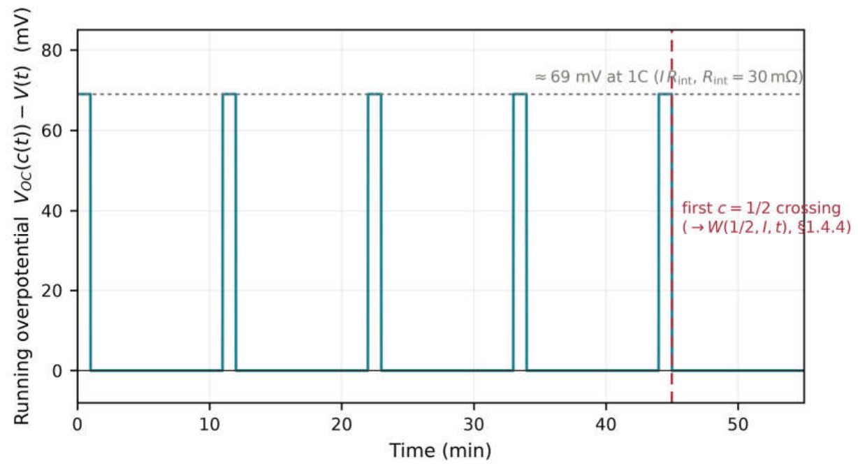
The driving term is the instantaneous irreversible heat generation rate (Figure 1.2), defined at every instant of the discharge trajectory. At crossings — and at those crossings only — the anchor-1 identity of §1.4.4 identifies this quantity with , converting the running overpotential at the symmetry composition into the Mahler-decomposition reaction-work observable.
Time series of the running overpotential (the elected open-circuit voltage along the discharge minus the measured terminal voltage) during a GITT pulse-and-rest protocol. The signal rises to about 69 millivolts during each 1C current pulse and returns to zero during rest. A dashed vertical line marks the first composition-midpoint crossing where the anchor-1 identity applies.
Figure 2.
Running overpotential during a GITT pulse-and-rest protocol, illustrating the driving term of Eq. (13). The quantity is defined at every instant of the discharge — during current pulses (~69 mV at 1C for the A123 26650 with m) and during rest periods (returns to zero as the cell relaxes toward the elected OCV). The dashed red line marks the first crossing, at which the anchor-1 identity of §1.4.4 identifies the running overpotential value with the Mahler-decomposition observable . Analytical/synthetic supporting illustration, not measured data.
Figure 2.
Running overpotential during a GITT pulse-and-rest protocol, illustrating the driving term of Eq. (13). The quantity is defined at every instant of the discharge — during current pulses (~69 mV at 1C for the A123 26650 with m) and during rest periods (returns to zero as the cell relaxes toward the elected OCV). The dashed red line marks the first crossing, at which the anchor-1 identity of §1.4.4 identifies the running overpotential value with the Mahler-decomposition observable . Analytical/synthetic supporting illustration, not measured data.
This identification is an observability statement at the anchor: the running quantity that drives Eq. (13) everywhere along the discharge is, at , the same object that the anchor-1 identity licenses as . The identification is pointwise in composition. It does not extend to a running function of composition; it identifies the anchor value with a physically meaningful term in the bivariate decomposition. The lumped instrument does not depend on the anchor-1 identification to run — it runs on the elected OCV curve and the measured terminal voltage directly. The anchor identification is what makes the driving term physically meaningful at the anchor point for Section 5’s mechanism-attribution language.
Two clarifications are essential. First, is not the actual cell temperature; it is the temperature the lumped model predicts under its constitutive assumptions (lumped thermal mass, single , no spatial resolution, no thermal gradients within the cell, no lumped-model-external heat sources or sinks). Second, the elected OCV curve enters Eq. (13) as a reference input — a curve, not a scalar — spanning the full composition range the discharge traverses. The framework’s election is therefore an election of the whole curve, not just its value at the anchor. The instrument does not attempt to close a coupled electrochemical–thermal system; it integrates the thermal side under whatever the voltage side is producing at each instant.
The local thermal constraint. For a given parameter vector and control setting, the framework evaluates one thermal constraint: the simulated T̂(t) from Eq. (13), driven by the I(t) and V(t) records against the elected V_OC(c(t)), should stay within a captain-specified band ΔT_suff of the ambient setpoint T_surr over the observation window. This is a single local constraint evaluation, not a terminal verdict on the experiment: the instrument returns the full parameter vector, the residual signatures, the constraint margin max|T̂— T_surr| relative to ΔT_suff (and to the half-band), and a per-constraint flag — thermal constraint satisfied when the margin is within band, thermal constraint violated when it is not. A satisfied thermal constraint at one operating point neither proves global feasibility nor, when violated, proves global failure; it is one coordinate in the captain-directed iterative feasibility search of §2.6.
The local thermal band ΔT_suff is set as a two-sigma criterion on the thermal noise floor: with a per-metric thermal resolution of σ_T = 1 K for room-temperature GITT, the declared band is ΔT_suff = 2σ_T = 2 K, and the systematic-offset sub-case threshold is the corresponding half-band 0.5·ΔT_suff = 1 K. The 2σ/2 K value is the local in-range test applied at each iteration; it is a constraint threshold, not the global stopping rule of the search.
Multi-curve Figure 1.3: a captain-declared bounded parameter search over convective cooling strength h_c for a 1C continuous discharge of the A123 26650 cell, with heat-transfer area A_h = 4.2e-3 m^2 and all other operating and model inputs fixed. Panel (a) overlays simulated cell-temperature trajectories T_hat(t) from Eq. (13) against the shaded 2 K local thermal band of Eq. (14) for h_c = 10, 15, 35, 40 and 60 W m^-2 K^-1 (G = h_c A_h = 0.0420, 0.0630, 0.1470, 0.1680, 0.2520 W/K). Maximum excursions max|T_hat - T_surr| are 4.9127 K, 3.9293 K, 2.1136 K (local thermal constraint violated) and 1.8918 K, 1.3349 K (local thermal constraint satisfied). Panel (b) is the search locus max|dT|(h_c): the crossing of the 2 K band gives a model boundary h_c* ~ 37.42 W m^-2 K^-1 (G* ~ 0.1572 W/K). This boundary is a model-implied cooling-design requirement under the synthetic operating case, not hardware validation and not an experimentally established practical limit; inferred h_c is distinct from a realizable cooling-control design. The figure shows how a local violation initiates bounded revision and rerun until the constraint is satisfied or only an impractical/unphysical solution remains. Analytical/synthetic supporting illustration, distinct from the GITT Case 3. 2-sigma criterion sigma_T = 1 K, band 2 K preserved.
Figure 3.
Bounded cooling-strength search for a 1C continuous discharge of the A123 26650 cell, all other operating and model inputs fixed (heat-transfer area A_h = 4.2×10⁻³ m2). (a) Simulated cell temperature T̂(t) from Eq. (13), driven by the actual I(t) and V(t) records against the elected V_OC(c(t)) (Safari–Delacourt [10]), overlaid for a captain-declared illustrative grid of the convective heat-transfer coefficient h_c = 10, 15, 35, 40, 60 W·m−2·K−1 (G = h_cA_h = 0.0420, 0.0630, 0.1470, 0.1680, 0.2520 W/K) against the shaded 2 K local thermal band of Eq. (14). Maximum excursions max|T̂−T_surr| are 4.9127 K, 3.9293 K, 2.1136 K (local thermal constraint violated) and 1.8918 K, 1.3349 K (local thermal constraint satisfied); the h_c = 15 W·m−2·K−1 curve is the natural-convection case (h_cA_h ≈ 0.063 W/K, Forgez et al. [12]) that peaks at ≈28.9 °C near t ≈ 33 min (ΔT_max ≈ 3.93 K, violated). (b) Search locus max|ΔT|(h_c): the response crosses the 2 K band at a model boundary h_c* ≈ 37.42 W·m−2·K−1 (G* ≈ 0.1572 W/K). This boundary is a model-implied cooling-design requirement under the synthetic operating case — not hardware validation and not an experimentally established practical limit; the inferred h_c is a model coefficient, distinct from a realizable cooling-control design. Analytical/synthetic supporting illustration, distinct from the GITT Case 3.
Figure 3.
Bounded cooling-strength search for a 1C continuous discharge of the A123 26650 cell, all other operating and model inputs fixed (heat-transfer area A_h = 4.2×10⁻³ m2). (a) Simulated cell temperature T̂(t) from Eq. (13), driven by the actual I(t) and V(t) records against the elected V_OC(c(t)) (Safari–Delacourt [10]), overlaid for a captain-declared illustrative grid of the convective heat-transfer coefficient h_c = 10, 15, 35, 40, 60 W·m−2·K−1 (G = h_cA_h = 0.0420, 0.0630, 0.1470, 0.1680, 0.2520 W/K) against the shaded 2 K local thermal band of Eq. (14). Maximum excursions max|T̂−T_surr| are 4.9127 K, 3.9293 K, 2.1136 K (local thermal constraint violated) and 1.8918 K, 1.3349 K (local thermal constraint satisfied); the h_c = 15 W·m−2·K−1 curve is the natural-convection case (h_cA_h ≈ 0.063 W/K, Forgez et al. [12]) that peaks at ≈28.9 °C near t ≈ 33 min (ΔT_max ≈ 3.93 K, violated). (b) Search locus max|ΔT|(h_c): the response crosses the 2 K band at a model boundary h_c* ≈ 37.42 W·m−2·K−1 (G* ≈ 0.1572 W/K). This boundary is a model-implied cooling-design requirement under the synthetic operating case — not hardware validation and not an experimentally established practical limit; the inferred h_c is a model coefficient, distinct from a realizable cooling-control design. Analytical/synthetic supporting illustration, distinct from the GITT Case 3.
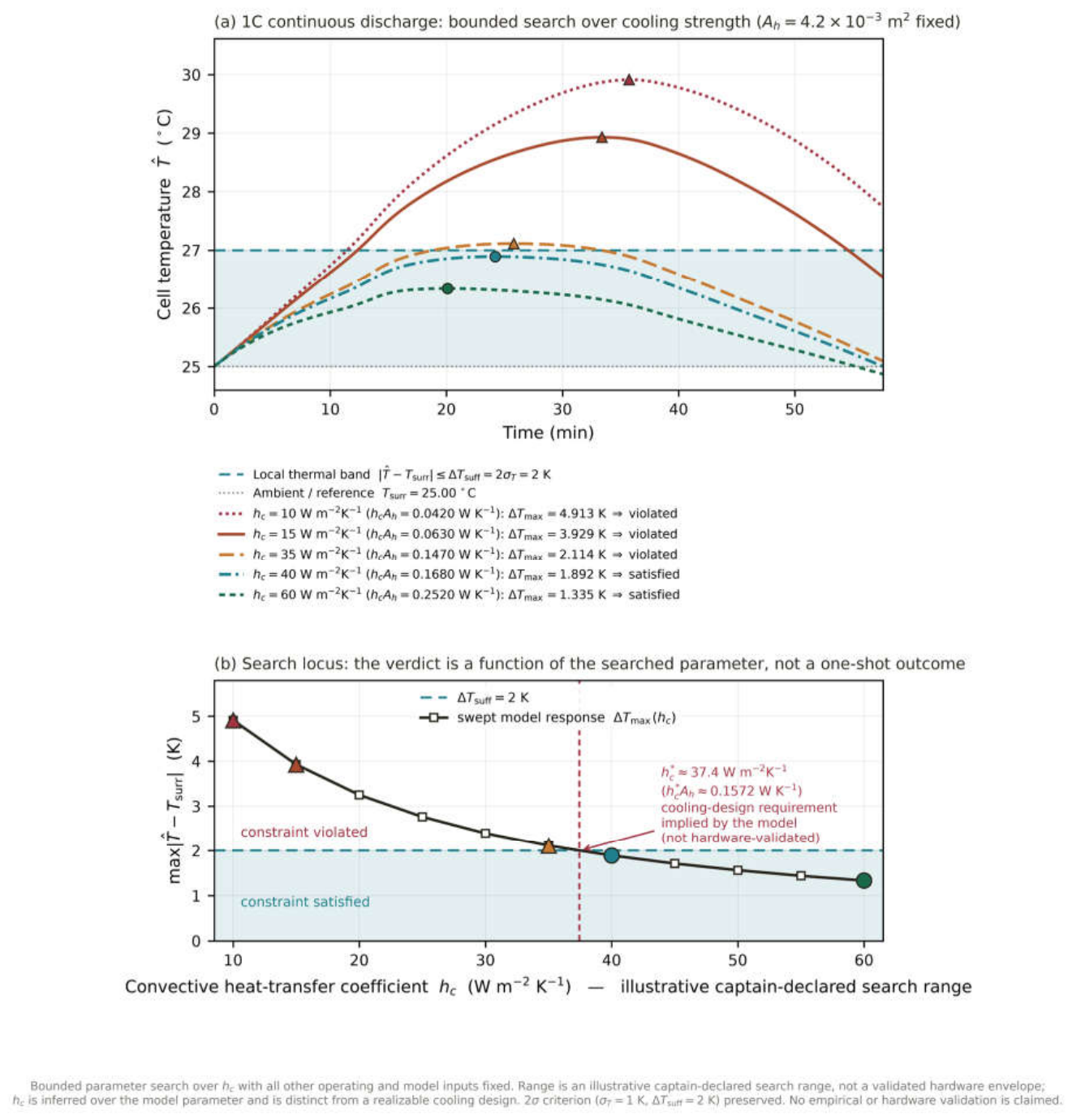
Figure 1.3 makes the iterative character of the local thermal constraint explicit. Reading a single trajectory — for example the natural-convection h_c = 15 W·m−2·K−1 curve, whose 3.93 K excursion violates the 2 K band — is one local constraint evaluation, not a terminal verdict. A violation initiates a bounded revision-and-rerun search: with A_h and all other inputs held fixed, the captain sweeps h_c across an illustrative declared grid (here 10–60 W·m−2·K−1) and reruns Eq. (13), and the local flag flips from violated to satisfied as the modelled cooling strength increases (panel b). The band crossing at h_c* ≈ 37.42 W·m−2·K−1 (G* ≈ 0.1572 W/K) is therefore a model-implied cooling-design requirement for this synthetic operating case, not a hardware-validated or experimentally established limit. Two distinctions matter here. First, the h_c that the lumped balance infers from an observed thermal record is a model coefficient describing the cell as observed; the h_c the search identifies as needed to satisfy the band is a candidate cooling requirement that a realizable cooling-control design (a fan, a coolant loop, a duty-cycle limit) would have to deliver — the algorithm does not change a physical coefficient by fiat. Second, the search terminates by the stopping rules of §2.6.1: it ends when the constraint is satisfied within captain-declared parameter bounds and practical limits, or when the only solutions that would satisfy it require an impractical or unphysical h_c — in which case the outcome is reported as infeasible rather than forced.
What a satisfied local thermal constraint delivers. When the search reaches an h_c that keeps T̂(t) within the 2 K band over the window (e.g. h_c ≥ 40 W·m−2·K−1 in
Figure 1.3), the operating point is inside the envelope in which:
- The rest voltage measured at the end of each GITT rest step is recoverable as the cell’s open-circuit voltage at the current composition, within the lumped model’s stated limitations.
- The symmetry-point value at each crossing is recoverable as the input to the Mahler-grounded identity of §1.4.4, again within the model’s stated limitations.
- The Arrhenius coupling of the exchange current to particle temperature, which is the mechanism of thermal feedback (H2,thermal, §5.3), is suppressed by construction — the local thermal constraint holds the cell within a band tight enough that the Arrhenius shift is small relative to the R8 discrimination threshold.
The framework does not claim that sufficient eliminates thermal effects
at the microscopic level. It claims that sufficient places the operating
condition inside the envelope in which the voltage-side signatures of
concentration polarization (§5.1) and phase morphology (§5.2) can be
discriminated without confounding from thermal feedback. §5.3’s discrimination
of H2,thermal exploits this: at sufficient the thermal-feedback
signature is absent by construction; deliberately reducing below the local thermal
threshold is the mechanism by which the framework provokes the signature for
R11 discrimination (§5.3.4).
Failure of the local thermal constraint When Eq. (14) fails over an observation window — excursions exceed at any point — the framework flags the operating condition as outside
the local thermal-constraint band and invokes a failure-mode diagnostic.
The diagnostic uses three quantities computed over the current rolling window
(whose length is a few multiples of the characteristic lumped-thermal time
constant ):
- Mean deviation: averaged over the window, indicating whether the local thermal-constraint failure is a systematic offset (constant thermal load, mischaracterized or , or a slowly-drifting external condition the model does not represent).
- RMS deviation: the root-mean-square of over the window, quantifying the magnitude of the excursion.
- Correlation of residuals with current: the Pearson correlation of with the drive-cycle current over the window, indicating whether the local thermal-constraint failure is current-coupled (spatial thermal gradients, current-dependent contact resistances, or thermal effects the constant- assumption does not capture).
These three quantities are diagnostic sub-cases of a violated local thermal constraint; they identify why the current h_c fails the local thermal constraint, not the routine tracking behavior of the lumped model against a measured thermal record. Their role is to inform captain review when the local thermal constraint is not met, so that a bounded feasibility update can move the operating point back inside the band (by increasing h_c, reducing the current-magnitude of the pulse protocol, or extending rest steps) before attribution is acted upon — each such update being one iteration of the search of §2.6.1. When the local thermal constraint is satisfied these quantities are not required and are not routinely reported.
What the instrument does and does not claim. The lumped instrument does not claim that is the actual cell temperature. It claims that is the lumped model’s prediction under its constitutive
assumptions, and that when this prediction remains within of the setpoint, the operating condition is inside the envelope
in which the voltage-side observables the framework depends on are clean.
The instrument does not claim that’smechanism attributions are validated by the thermal side.’sattributions are voltage-derived and stand or fall on the voltage-side discrimination heuristics. The lumped instrument provides a running local thermal-constraint flag on the operating-condition dimension, which is a distinct question from the mechanism-attribution dimension. When the local thermal constraint is satisfied the mechanism attribution is reported at its intrinsic confidence. When the local thermal constraint is violated the mechanism attribution may still be correct, but the framework flags the possibility that the voltage-side signatures are being interpreted in a thermal context the local thermal constraint does not guarantee is clean, and refers the operator to the failure-mode diagnostic above.
Energy-closure admissibility. The lumped instrument also carries an integral energy bookkeeping that gates every candidate simulation before any physical interpretation. The framework does not equate the full terminal electrical energy directly to heat. The model heat source is, with (dissipative, always positive) and= +I·T·dU/dT (the reversible/entropic term, signed as coded,
following the digitized Forgez et al. dU/dT), so only the generated heat —
not the terminal electrical work — enters the thermal balance. Integrated over
the discharge window, generated heat must equal sensible storage plus
convective rejection:
where is the integrated convective rejection, Δ = M [T ̂ ( )−T ̂ (0)] is the sensible-storage change (nonzero because the final
temperature need not return to ambient), and is the closure residual. This is a solver/model energy closure —
it verifies the internal consistency of the numerical solution against the
declared model’s own bookkeeping, and makes no claim of experimental or
hardware closure. Using a first-law energy balance as an admissibility screen
on signals has an established precedent [13];
here the balance screens the internal consistency of the numerical solution — a
model/solver closure test — rather than validating measured data against
hardware.
Framework order. The energy-closure check therefore sits first in an explicit ordering applied to each candidate simulation: (i) the energy-closure/admissibility check — a candidate whose is not within solver tolerance is rejected as a
computational/model inconsistency before any physical reading; (ii) the local
2σ/2 K thermal-constraint evaluation of Eq. (14); (iii) the coupled physical
and practical feasibility assessment (are the required coefficients physical
and the implied cooling demand realizable?); and (iv) the captain-directed
bounded update and rerun of §2.6.1. Only admissible candidates — those that
close energetically — are eligible for the thermal and feasibility stages.
Audited closure of the
Figure 1.3 sweep. The Figure 1 .3 sweep is audited under this gate. At the model boundary
* = 37.42 W·m−2·K−1
(G =
= 0.1572 W/K):= 548.47 J,= 155.26 J,= 703.73 J,= 700.18 J, Δ= 3.55 J, closure residual= −1.66×10⁻¹¹ J (−2.36×10⁻¹² % of
), with max|ΔT| = 1.9999 K (local
thermal constraint satisfied). At the first satisfying grid point
= 40 W·m−2·K−1 (G = 0.168 W/K):= 703.69 J,= 703.32 J, Δ= 0.37 J,= 3.71×10⁻¹¹ J, max|ΔT| = 1.8918 K (satisfied).changes only slightly across the sweep becausedepends on the temperature trajectory while
·t is fixed; the sensible-storage term
is retained precisely because the final temperature differs from ambient. Every
plotted curve in Figure 1.3 closes energetically to this precision; the satisfying curves additionally meet
the 2 K constraint, so the
sweep is a search over admissible candidates in which the
thermal constraint, not energy closure, is the binding condition. Exact values
are retained in the reproducibility package.
1.5. Epistemic Discipline: What the Framework Claims and Where It Stays Silent
The four grounding layers assembled in §1.4 — Mahler’s bivariate first law, the regular-solution symmetry of LiFePO4 at c = 1/2, Bazant–Zeng heterogeneous kinetics, and the lumped cell-level enthalpy balance of §1.4.7 — do not, taken together, constitute a closed-form model of the cell. They are not offered as one. This section states, plainly, the epistemic discipline that governs what the framework claims and where it refuses to speak.
The framework is a reasoning instrument, not a forward simulator. Its purpose is to support attribution decisions on measured records under a defined protocol — to discriminate among
concentration polarization, phase morphology change, and thermal feedback as
candidate mechanisms for observed voltage residuals. It does not attempt to
predict from first principles. It does not attempt to recover the
microscopic partition of instantaneous electrical power between reversible
reaction work and irreversible heat. It does not offer the exponential
temperature profile that follows from the first-order enthalpy balance of
§1.4.7 as the cell’s true thermal response. That profile is the coarsest
bookkeeping the first law admits when the cell is treated as a single lumped
thermal capacity — it is a chosen frame of reference, an elected instrument, and
its exponential shape is a mathematical consequence of the election rather than
a claim about the battery.
This discipline is required by the physics, not chosen by preference. Heat and work are path functions. For a real battery under a real current schedule, the path along which is accumulated and the path along which is extracted are not the same path in time. The work extraction tracks the current schedule directly; the heat dissipation lags on the cell’s thermal time constant , which for the A123 26650 format lies in the range of several
minutes to tens of minutes. Any closed-form model that partitions instantaneous
electrical power into a “heat now” component and a “work now” component is
forcing a synchronization between and that the physics of the cell does not provide. Every reach for
such a closed solution is, in this framework, a failure mode — not because
closed solutions are inherently wrong, but because for this class of coupled
electrochemical–thermal system the closed solution demands a partition that is
not observable at the cell terminals and is not derivable from the four
grounding layers of §1.4.
The framework works, and can only be defended as working, because it operates at points where path-function ambiguity vanishes. There are exactly two such points in the present treatment:
- The symmetry-point identity at (§1.4.4). At the composition midpoint of the LiFePO4 regular-solution model, the excess-enthalpy contribution to the kernel drops out on symmetry grounds, and the voltage-side observable becomes identifiable with a per-charge reaction-work field. The partition of terminal voltage into equilibrium and non-equilibrium components is clean at this point because the state variable is fixed by construction, and the path-dependence of the surrounding trajectory does not enter the identity. Everywhere else along the composition trajectory, the partition is not clean and the framework does not attempt to make it clean.
- The rolling-window first-law closure (§1.4.7). Integrated over a window of a few , the first law closes: the net electrical energy input over the window equals the net heat accumulated plus the net work extracted, up to the boundary flux of . The time-zone mismatch between prompt work and lagged heat integrates out over the window. The lumped instrument’s role is to check that this integrated balance closes — the local thermal constraint trace, which would require synchronizing and pointwise and is not defensible.
The observable and its constraint. The two anchors are not two independent statements about the cell. Anchor 1 is the observable — the value of the terminal voltage at that appears in any
discharge record, whether or not the record’s author knew to look for it.
Anchor 2 is the constraint that licenses interpreting that observed value as
the symmetry-point identity’s rather than as a number
that merely occupies the corresponding slot in the spreadsheet. Anchor 2 does
its work through sufficiency: the assertion
that the cell has stayed inside the coarse-bookkeeping regime — no hot spots,
no thermal-runaway drift, no departure from the single-node lump — under which
the particle-population state at cell-level SoC can be treated as
coherently at in the sense the
regular-solution symmetry identity requires. Under this reading anchor 2 is not
a second observability guarantee. It is the domain of validity for anchor 1,
pulled back from the cell’s microstate — which the framework refuses to model —
into a condition the coarse instrument can check by first-law bookkeeping over
a rolling window. Operationally, the licensing condition takes the form of Eq.
(13), which integrates the running overpotential against the boundary flux
over time; anchor 2 asks not whether that ODE matches a measured , but whether the simulated stays inside the local
thermal band of Eq. (14) over the window that brackets the anchor observation.
Every that appears in a real
record carries this constraint whether or not it is stated. When has been sufficient over
the window that brackets the observation, the observed is licensed as the
symmetry-point identity’s and the
mechanism-attribution language of Section 5
applies to it. When has not been sufficient,
the observed number is a number in a spreadsheet with no further guaranteed
meaning; Section 5 ’s language is not licensed on it, and the framework’s mechanism
verdict is withheld. The two anchors are hinged. The framework has one
observable and one licensing condition, and the closure discussion that follows
is the operational form the licensing condition takes.
The closure the second anchor asserts is a closure by construction. The lumped enthalpy balance of §1.4.7 is written as a first-law statement — its integrated form closes to numerical precision over any window because we have written it to close, not because the cell has been observed to close it. This is not a weakness of the anchor; it is what the anchor is. The first-order temperature response is the ODE’s output under the elected OCV curve, the measured current, and the measured terminal voltage as inputs. The elected OCV curve enters the balance as a running reference against which the
driving term is formed pointwise in time; it is a designated input, not an
approximation of the integration region. Refining either — a more accurate
thermal capacity, a more empirically anchored OCV, a higher-order thermal model
— would sharpen the shape of the integration region but would not alter what
the second anchor claims. What the second anchor claims is that the first law
of thermodynamics is enforced as the interpretive frame for the cell’s behavior
over the window. The work of attributing this enforcement to the real battery —
not merely to the ODE we have written — is done by the local thermal constraint
. When is asserted to be sufficient, the assertion is that the
coarse-bookkeeping regime in which the first law admits this lumped statement
is the regime in which the cell is operating. Sufficiency is the physical
claim; the closure is bookkeeping in support of that claim. This is why the
election of a designated OCV in §1.4.4 and here — the Safari–Delacourt
regular-solution form retained across the treatment — is not a limitation to be
relaxed by fitting to measured data. Chasing a “better” OCV, or a temperature
profile that reproduces a measured more faithfully, would be the closed-form ambition this section
has refused: it would substitute approximation-refinement for first-law
enforcement and would displace sufficiency as the load-bearing physical commitment. The second
anchor stands on election plus first-law enforcement plus sufficiency. Improvements in the accuracy of the integration
region change the numbers on the page; they do not change what the framework
says about the battery.
Everywhere else, the framework stays silent. This silence is not an omission awaiting future refinement; it is the framework’s claim. The paper does not offer a mechanism decomposition for outside the neighborhood of . It does not offer a pointwise thermal partition. It does not
offer a closed-form prediction against which the cell’s measured can be scored. It does not offer a fit of from the shape of the temperature transient — only the
sufficiency check on whether the integrated balance closes within an admissible
band.
The discipline extends to a strict admission rule for additional anchors. A third anchor — a third point in the composition–current–temperature configuration space at which path-function ambiguity provably vanishes and a new observable becomes identifiable — would, in principle, extend the framework’s non-silent domain. The present treatment does not claim such a third anchor. If and only if such an anchor is discovered and defended on the same grounds as the two established here — symmetry-based partition cleanliness at a fixed state, or integrated closure over a defined window — will the framework speak beyond §1.4.4 and §1.4.7. The paper offers no provisional third anchor, no candidate under investigation, no soft extension of the framework’s voice. Silence is preferred to speculative extension.
The election of OCV as an ideal thermodynamic cycle, on which the equilibrium reference in §1.4.4 depends, is disclosed here as an election rather than a discovery. The regular-solution OCV is a designated reference against which the cell’s terminal
voltage is measured; it is not claimed to be the cell’s true equilibrium
potential in an absolute sense. The framework operates by measuring departures
from this elected reference under conditions in which the reference is
well-defined. Its status as an election, rather than a fact recovered from the
cell, is what allows the framework to remain honest about its scope: at the reference is defensible by the symmetry construction; over
the rolling window the reference is defensible by first-law closure; elsewhere
the reference is a convenience, and the framework does not push it beyond
convenience.
This is a reasoning framework in the classical sense: it uses the coarsest bookkeeping compatible with the physics, at the two points where the bookkeeping identifies observables cleanly, and it refuses to substitute closed-form ambition for the acknowledgment that path functions on decoupled timescales cannot be recovered from cell-terminal measurements. What it produces is an attribution verdict on a measured record, with an accompanying local thermal-constraint flag on the thermal side, and nothing else. What it does not produce is a simulation of the cell, and it should not be read as one.
Accordingly, the paper distinguishes local constraint states from global outcomes throughout. A local flag (thermal constraint satisfied or violated at one operating point; an R-rule positive or negative) is an observation; the global outcome of the study — feasible, infeasible, or indeterminate — is reached only through the captain-directed iteration of §2.6.1, and no single local flag is reported as if it were that global outcome.
2. The Dialogue Process and Its Discipline
2.1. A Taxonomy of Moves
The dialogue documented in this paper consisted of exchanges between the human captain and the AI expert system, conducted over multiple threads spanning June 16 through July 10, 2026, and preceded by a prior thread that terminated on May 1, 2026 with a structured handoff document. The exchanges resolve into six categories of move, the distribution of which across the two participants is asymmetric and methodologically significant.
A generation move proposes a structural candidate — a decomposition, functional form, regime partition, condition set, or hypothesis. Generation moves are evaluated against constraints external to the move (dimensional consistency, asymptotic compatibility, prior commitments, domain plausibility) and are not adopted by default. Generation is the expert system’s primary substantive output.
A retrieval move obtains material external to the immediate dialogue: a published equation, workspace file, web page, or prior handoff. Retrieval is constrained to canonical or captain-identified sources and its products are verified. One instance is the retrieval of Equation (4.1) from Zeng and Bazant [1] after the captain pointed to the inverse hyperbolic sine term — performed against the canonical source rather than reconstructed from parametric memory.
A verification move tests a retrieved or generated object against an independent criterion: a derivation, a limit, a symmetry, a consistency condition. Verification is the operation by which retrieval is converted into warranted use.
A structural-check move tests whether a proposed object satisfies constraints not retrieved from any source but required by the framework’s coherence: dimensional homogeneity, asymptotic compatibility, partition uniqueness, regime consistency. Structural checks are the expert system’s distinctive contribution.
An error move generates or asserts something that is, on subsequent inspection, false or inappropriate. Errors are categorized in §2.4 below and are documented rather than concealed.
A correction move identifies an error and replaces the erroneous object with a revised one. Corrections may be initiated by either participant but are predominantly captain-initiated in the present dialogue.
2.2. The Asymmetric Distribution of Moves
The distribution of moves across the two participants in this dialogue is not symmetric and the asymmetry is methodologically load-bearing.
Generation was performed predominantly by the expert system. Retrieval was distributed but through different mechanisms — the captain retrieved domain knowledge from expertise, the AI retrieved canonical equations and prior artifacts. Structural checking and errors were predominantly the expert system’s; corrections were predominantly captain-initiated; and final structural selection was performed exclusively by the captain.
Every commitment that the framework in Section 4 and Section 5 depends on — the choice of OCV as the equilibrium reference; the assignment of c = 1/2 as the symmetry anchor; the rejection of the polynomial reduction as off-topic; the framing of the paper as methodological rather than electrochemical; the identification of W as per-charge reaction work per §1.4.4; the treatment of the enthalpy balance as a running instrument per §1.4.7; the refusal to derive the microscopic partition between heat and work — was a captain selection from among expert-system-generated or expert-system-surfaced candidates. The expert system did not, in this dialogue, exercise final structural authority on any commitment.
2.3. The Handoff Mechanism as Anti-Hallucination Scaffold
The dialogue inherits an explicit structured artifact from a prior thread: a handoff document authored by the captain at the end of the 2026-05-01 LFP review thread, with successor handoffs at each subsequent thread boundary. The handoff is not merely a summary; it is an active scaffold against the principal failure modes of expert-system reasoning in extended dialogue. Four mechanisms are identifiable.
Locked decisions constrain the generation space. The handoff enumerates explicit “decisions made” in prior threads. When a new thread’s opening message contradicts a locked decision, the expert system detects the tension and surfaces it to the captain as an explicit choice rather than silently overriding.
Deferred questions block premature closure. The handoff explicitly enumerates open items from prior threads. By naming what is not settled, the handoff converts what would otherwise be silent gaps into observable unresolved items.
Epistemic preferences install a corrective posture before any specific claim is generated. The handoff states, as captain preferences observed in prior threads, requirements for push-back on overclaims, demand for observable grounding, rejection of hand-picked structural ansätze, and honest scholarship without fabricated quotations or page references. These statements operate as behavioral constraints on subsequent expert-system generation.
File pointers and canonical citations provide retrieval anchors. The handoff identifies specific source documents as canonical, converting retrieval from an open-ended search problem into a targeted fetch with verifiable provenance.
The four mechanisms operate jointly, with combined effect greater than any single one. The handoff is the principal anti-hallucination instrument identified in this case study. It is not something the expert system can produce for itself; it is a captain-authored artifact whose function depends on the captain’s authority to lock decisions, defer questions, state preferences, and identify canonical sources.
2.4. Observable Failure Modes and Their Detection
Four failure modes of the expert system are identifiable in the present dialogue’s record.
Failure mode 1 — premature definitional commitment under inadequate constraint. The expert system’s first substantive response offered a three-way taxonomy of “polarization” and asserted that polarization “is not a field.” This was wrong: the activation overpotential is a pointwise-defined field on the reacting surface in the Zeng–Bazant formulation. The captain detected it by invoking the sinh−1 term. Cost: ~2 turns.
Failure mode 2 — overcommitment to a retrieved object without scope analysis. After retrieving Equation (4.1), the expert system endorsed it as a working kernel and built a scoping decision tree on it. The endorsement was premature: the kernel’s uniform-composition assumption is most violated precisely at the symmetry point where it has its only clean operational reading. The captain detected it via the c = 0.5 symmetry observation. Cost: ~3 turns and a substantive reframing.
Failure mode 3 — generation drift under under-constrained prompts. After the captain’s polynomial-substitution suggestion, the expert system produced an extended polynomial-versus-rational approximation analysis: not factually wrong, but off the load-bearing path. The captain corrected it with “we are getting off track.” Cost: ~2 turns.
Failure mode 4 — generation under structural commitment without audience constraint. Instructed to draft the first attribution subsection, the expert system produced a technically sound but too cognitively dense draft for a single reviewer reading. Unlike FM1–FM3, it violated no given constraint; it failed against one it had not been instructed to represent — cognitive accessibility to a peer reviewer. The captain detected it by direct reviewability judgment, and directed a two-step compression (four equally weighted rules reduced to two primary rules plus two secondary corroborators, then condensed into three compact decision tables) that cut the section’s word count by ~60% while preserving thermodynamic rigor and structural fidelity.
FM4 is more significant methodologically than FM1–FM3. FM1–FM3 are failures within constraints the expert system could in principle represent (and which the §2.3 handoff mechanism partially installs). FM4 fails against a constraint not naturally representable within structural bookkeeping at all: audience cognition is not a thermodynamic identity, dimensional consistency, asymptotic limit, or prior commitment — it is a property of the eventual reader.
Scope correction (distinct from FM1–FM4). The dialogue also exhibited one instance of a structurally different captain intervention: a scope correction in which the captain narrowed the paper’s hypothesis space mid-draft, without responding to any specific AI failure.
SC1 — Marcus exclusion (2026-06-19). While draftingSection 5.2, the captain ruled the Marcus/coupled ion–electron transfer hypothesis out of scope entirely. The ruling did not respond to any specific AI failure — the drafts satisfied all binding decisions — but narrowed the paper’s claims, retiring a hypothesis broader than the paper would defend.
SC1 shows captain authority operating at multiple levels: not only corrective filtering of specific AI failures but scoping authority that narrows or expands the dialogue’s claims independent of AI performance. The expert system can satisfy every committed constraint and still carry material the captain decides, on independent grounds, to remove.
Pattern statement. Across all four failure modes, the expert system generated material that was structurally well-formed and locally plausible but globally inappropriate to a required constraint. In FM1–FM3 the constraint was one the AI could in principle represent, and captain filtering operated within the dialogue’s structural commitments to catch it; in FM4 the constraint — reviewer cognitive bandwidth — was outside the AI’s native access, and captain filtering installed it after the fact. In no documented case did the expert system detect the inappropriateness before captain intervention.
2.5. Model Identification and Reproducibility Limits
The dialogue documented in this paper was conducted on the Perplexity Computer agent platform, accessed by the captain through the platform’s standard web interface. The platform deploys large language models from multiple providers and routes individual conversation turns through models selected by platform-internal logic that is not exposed at the conversation level. The specific large language model serving each turn of the present dialogue is therefore not introspectively accessible from inside the dialogue.
The platform is Perplexity Computer. The captain is Roger Painter, operating from Nashville, Tennessee, with an Enterprise Max subscription. The dialogue spans June 16, 2026 to July 10, 2026 across multiple threads, with a prior thread terminating May 1, 2026 having produced the initial handoff document.
The reproducibility of this case study rests on three artifacts: the present paper, the captured thread transcripts, and the succession of handoff documents. Reproducibility does not rest on any guarantee of model identity at the turn level. The opacity of the underlying model is a condition of the platform under which the dialogue occurred, and it is documented as such.
2.6. Synthetic-Signal Generation and Computational Method
The signals analysed in Section 6 are produced by a small, fully owned Python package (the reproducibility package accompanying this paper). The method is deliberately transparent and deterministic. Each case is defined by a human-readable configuration file that fixes the GITT protocol (pulse current, pulse and rest durations, pulse count, sampling interval, starting state of charge), the lumped thermal parameters, the sufficiency criterion, the injected signature, and a random seed; identical seeds reproduce identical output bit-for-bit.
Each generated record is a time series on a common channel schema: time, applied current, a pulse/rest indicator and pulse index, state of charge, cell temperature (in kelvin and °C and as a deviation from ambient), the open-circuit voltage from the Safari–Delacourt LiFePO4 form, the terminal voltage, and the reaction-work residual W_res that carries the diagnostic signature. The temperature channel is integrated from the single-node lumped balance of Eq. (13) with an ohmic term, an entropic term using a digitized approximation of the Forgez (2010) dU/dT curve, and one declared residual heat-coupling term; the open-circuit-voltage structure is the analytical LiFePO4 form. These are declared modeling constraints, not claims of experimental fidelity.
A signature module injects one known mechanism per case—concentration-polarization memory, a plateau-geometry tilt, a negative sign-and-decay thermal residual, or none (a noise-only negative control)—on top of Gaussian measurement noise at a declared amplitude. The heuristic-evaluation module applies the manuscript R-rules that are decidable from a single GITT record (R3, R6, R8) and reports both their numerical diagnostics and their boolean verdicts, together with the 2σ local thermal-constraint flag for the current operating window.
2.6.1. Iterative Constraint Balancing and Feasibility Search
The single-record evaluation above is one iteration of a human-guided feasibility search, not a terminal classifier. In each iteration the captain (i) generates or observes the synthetic BMS-like signals for a given parameter vector and control setting; (ii) evaluates the coupled thermal, kinetic, and mass-transfer behaviour through the residual signatures and the R-rules together with the local thermal-constraint margin of §1.4.7; (iii) identifies which conditions are violated or only weakly constrained; (iv) proposes a bounded, physically defensible update to parameters or to the control/cooling setting; and (v) reruns and compares. The loop repeats until a global outcome is reached.
Three global outcomes are distinguished, and are kept separate from any single local flag. (a) Feasible (success): at least one jointly admissible solution is found in which every constraint is satisfied, the required heat-transfer coefficient or control demand is practical, and all parameters remain physical. (b) Infeasible (failure): the bounded search is exhausted, or the only solutions that fit the data require an impractical heat-transfer coefficient, non-physical parameters, or mutually contradictory settings. (c) Indeterminate: the available observations do not constrain the question, and a more informative experiment or operating condition is required. A single crossing of the 2 K local thermal band is never, by itself, a global failure; it is one constraint evaluation that informs the next bounded update.
Software scope (stated accurately). The accompanying package is a single-pass diagnostic and rule-evaluation tool: for one configuration it generates the record, evaluates R3, R6, and R8, computes the local thermal-constraint margin and flag, and writes the parameter vector, residual signatures, margins, and flags to machine-readable CSV and JSON. It does not contain an automated multi-iteration optimizer. The iteration across configurations — choosing the next bounded update, re-running, and comparing — is performed by the human captain, who edits the configuration files; the software provides the per-iteration diagnostics on which those decisions rest.
Stopping criteria and audit trail. The search terminates under captain-declared, configured limits: the parameter bounds and practical heat-transfer/control limits recorded in each case configuration; a no-improvement/convergence criterion (successive bounded updates cease to reduce the active constraint violation); and a captain-declared maximum iteration count. The present study reports single-iteration evaluations, so these limits are declared rather than exercised across many reruns. Every iteration is auditable: the configuration (with its fixed seed), the resulting margins and flags, and the captain’s stated reason for each parameter or control update are recorded, so the path from observation to update to outcome is fully traceable.
3. Implications for AI-Assisted Reasoning in Partially Closed Physical Theories
3.1. What the Case Study Establishes, and What It Does Not
TheSection 2 dialogue produced a falsifiable artifact within a finite number of exchanges between a human domain expert and an AI expert system, under the discipline of handoff documents inherited across threads. The case study establishes that such a partnership is possible in at least one realistic technical dialogue, that its products are checkable against the domain’s own standards, and that its failure modes are observable and correctable under the described discipline. These are existence claims, not generalization claims.
The case study does not establish that AI-assisted heuristic reasoning will converge in every dialogue, on every problem, with every captain, or with every underlying language model. It does not establish that the asymmetric role distribution of §2.2 is optimal, that the handoff mechanism of §2.3 is sufficient, or that the failure modes of §2.4 are exhaustive.
3.2. Partially Closed Physical Theories as a Target Class
The LFP single-particle model belongs to a broader class of physical theories sharing three features: a rigorously derived closed regime, a known and characterized envelope of validity, and a practically important operating regime lying partly inside and partly outside that regime. Conjectured members include porous-electrode models beyond the dilute-solution and uniform-reaction limits, turbulent transport beyond the laminar regime, heterogeneous catalysis beyond the well-mixed limit, and ecological/epidemiological population dynamics beyond the mean-field approximation.
For such theories, the AI-assisted heuristic extension pattern documented in this paper offers a candidate methodology. The pattern proposes to anchor on the closed theory’s structurally clean points and to construct, through disciplined dialogue, a falsifiable extension whose deviation from the closed theory carries explicit operational meaning.
3.3. The Expert System as Structural Bookkeeper
A specific claim the case study supports as plausible is that the AI expert system’s principal value in such dialogues is not as a generator of finished models but as a structural bookkeeper across extended sequences of moves — tirelessly tracking dimensional consistency, asymptotic compatibility, partition uniqueness, regime consistency, and prior commitments, operations whose individual difficulty is low but whose sustained execution across many turns exceeds unaided human attention.
A corollary is that the value of the AI in such dialogues scales with the expert’s willingness to challenge AI generations. An expert who treats the AI’s generations as authoritative will inherit the AI’s errors. An expert who treats the AI’s generations as candidates for filtering will obtain a generator-and-checker partner whose limitations are predictable and whose products are checkable.
3.4. The Handoff Document as Transferable Artifact
The §2.3 handoff mechanism is, on this case study’s evidence, a non-trivial methodological contribution potentially transferable beyond the present application; its effectiveness rests on four components whose joint operation prevents identifiable failure modes.
A limitation is that the handoff operates on constraints the expert system can in principle represent — domain knowledge, prior commitments, epistemic preferences, canonical sources — and does not natively install constraints external to its structural bookkeeping, such as the reviewer cognitive bandwidth documented as FM4 in §2.4. A “scope priors” mechanism, in which the captain specifies audience-cognition and readability constraints in the handoff, is a candidate extension for further case studies.
3.5. The Opacity of the Underlying Model and Reproducibility
The case study argues that the appropriate response to model opacity is not model-level reproducibility — often unavailable in practice — but artifact-level reproducibility: the transcripts, handoffs, and published paper can be inspected, audited, challenged, and replicated by independent attempts on possibly different underlying models.
3.6. Limits of the Case Study and Directions for Further Work
Three limits should be stated explicitly. First, the dialogue involved an expert captain deeply familiar with the problem. Second, it was conducted in a specific tooling environment under specific institutional conditions. Third, its convergence is observable only in retrospect; the pattern’s behavior on non-convergent dialogues is not documented here.
A fourth limitation is that captain authority operates at two levels — corrective filtering of specific AI failures (FM1–FM4) and scoping-level narrowing of claims (SC1). The scoping level is not observable within a single turn; it depends on ongoing captain judgment about which claims to defend and produces interventions no AI failure could anticipate. Transferability to teams lacking a captain able to exercise scoping authority is an open question.
3.7. Summary of Implications
The case study demonstrates that a human domain expert and an AI expert system, under explicit role asymmetry and the discipline of structured handoff documents, can produce a falsifiable methodological framework for the heuristic extension of a partially closed physical theory.
The principal contribution is the pattern, not the framework. Its components — asymmetric role distribution between human authority and AI generation-checking, structured handoff documents as anti-hallucination scaffolds, explicit failure-mode cataloging, and artifact-level rather than model-level reproducibility — are offered as hypotheses worth testing in further case studies across domains, captains, and AI systems.
4. Reference Logic at the Symmetry Point
4.1. Why the Symmetry Point Is the Natural Reference
The Cahn–Hilliard reaction kernel of Zeng and Bazant [1] (Eq. 4.1) decomposes the single-particle voltage into a reference potential, a diffusional chemical potential μ̃(c̃), and a Butler–Volmer activation term whose exchange current is itself a functional of μ̃(c̃). For the regular-solution model characteristic of LFP, μ̃(c̃) vanishes identically at c̃ = 1/2 by symmetry. The expert system uses this collapse as its primary reference point.
The reference logic measures the Mahler non-equilibrium reaction-work field W(1/2, I, t) directly at the only point on the discharge curve where the bivariate kernel’s two fields decouple by construction (§1.4), and tests whether W so measured is consistent with the bare Butler–Volmer prediction W^BV(1/2, I, t) = (2k_BT/e)·sinh−1(I/2I0*). The C1–C5 conditions defined below are conditions on this directly observed thermodynamic field.
The framework’s reference logic operates on the voltage-derived observable W(1/2, I, t). Per §1.4.7, the framework runs in parallel a lumped enthalpy balance as a local thermal-constraint instrument , producing a simulated cell temperature from the actual drive-cycle current record and the
voltage-derived W. The instrument certifies over each observation window
whether the local thermal constraint stays within the captain-specified band of the ambient setpoint — and this local thermal-constraint flag
is reported alongside every attribution result per §5.4’s joint attribution
report.
4.2. The Reference Equilibrium and the Low-Current Calibration
The expert system establishes the equilibrium chemical potential field from a measured
open-circuit voltage curve:
(in absorbed voltage units per §1.4.3), with obtained from a Galvanostatic Intermittent Titration (GITT) protocol. The reference potential is fixed by the condition , i.e., .
A minimum current I_min = C/10 is assigned operationally as the validity threshold below which the system is in the equilibration regime and above which polarization is a response to driving.
The bare Butler–Volmer prediction at the symmetry point is defined as
where the single calibrated parameter I0* is the bare exchange current at the symmetry point, extracted from the lowest available current I1 ≥ I_min via the linear limit:
The operational procedure that converts an experimental GITT record into the
anchor-neighborhood residual consumed by the R-rule
battery of §5.1–§5.3 is stated as a five-step extraction pipeline in §6.0.1,
together with the anchor-neighborhood discipline that licenses reading as a continuous-time signal
over the composition window around each crossing.
4.3. The Deviation Metric
For each measured discharge at current I_j, the expert system extracts the cell voltage at the moment when the cumulative passed charge corresponds to average SOC c̄ = 1/2, computes the corresponding bare BV prediction, and computes the deviation ΔV_j ≡ V_j^obs - V_j^BV. The sign convention is such that ΔV_j < 0 indicates that the measured cell is more polarized than the bare BV prediction.
Under H0, W(1/2, I, t) is given by bare Butler–Volmer with constant I0* and is time-independent at fixed I. Under H1, W(1/2, I, t) carries the Zeng–Bazant coupling (1-c)·exp(αμ̃) via internal-gradient effects. Under H2, W(1/2, I, t) carries contributions from one or more of the non-Butler–Volmer mechanisms: concentration-polarization memory (H2,conc, §5.1), phase morphology change (H2,phase, §5.2), or thermal feedback (H2,thermal, §5.3). The kinetic saturation hypothesis (Marcus/CIET) has been excluded from scope per captain ruling SC1.
4.4. The Statistical Distinguishability Heuristic
The expert system declares the coupling term statistically distinguishable from noise when the following heuristic conditions are all satisfied:
- C1 — Monotonicity. The sequence {|ΔV_j|} ordered by I_j is monotonically non-decreasing, except for noise excursions within the per-rate noise floor σ_j.
- C2 — Sign coherence. All ΔV_j above the noise floor have the same sign.
- C3 — Threshold rate. There exists a threshold current I^† above which |ΔV_j| > k·σ_j for a chosen coverage factor k (default k = 3).
- C4 — Cross-rate consistency. Above I^†, the magnitudes |ΔV_j| form a smooth curve in I_j.
- C5 — Per-rate noise estimation. The noise floor σ_j at each rate is estimated from the residuals over a local SOC window (default: 0.45 ≤ c̄ ≤ 0.55).
4.5. Decision Flowchart
The reference logic is summarized as a four-step procedure:
- Establish V_OC(c) from GITT protocol; fix V^Θ ≡ V_OC(c = 1/2).
- Calibrate I0* from the linear limit at the lowest available rate I1 ≥ I_min.
- Compute the bare BV prediction V_j^BV at each available rate I_j; extract V_j^obs at c̄ = 1/2; compute deviations ΔV_j.
- Apply C1–C5; declare coupling distinguishable, falsify bare BV, or flag insufficient data.
5. Attribution Stage
5.0. The Attribution Stage: From Measured W to Mechanism Decomposition
The reference logic of Section 4 produces, when its conditions C1–C5 are satisfied, a tabulated set {(I_j, W(1/2, I_j, t), σ_j)} at the symmetry point and a binary declaration that the bare Butler–Volmer prediction for W is falsified by the data. Section 5 documents the framework’s attribution stage: the heuristic procedure by which the measured per-charge reaction-work field W(1/2, I, t) is decomposed into contributions from an enumerated set of mechanistic hypotheses, under qualitative reasoning and without parameter fitting. Combining a heuristic rulebase with qualitative-simulation predictions to produce partial or uncertain recognition rather than forced classification is a long-standing pattern in model-based diagnosis [14], as is transparent rule-style reasoning over model residuals that returns a multiple-valued outcome, including an explicit non-committal state [15].
The attribution stage operates on the symmetry-point-identified voltage-derived observable W per §1.4.4. In parallel, per §1.4.7, the framework runs a lumped enthalpy balance as a local thermal-constraint instrument , certifying over each observation window whether the local
thermal constraint of Eq. (14) holds. §5.4’s joint attribution report combines
the voltage-derived mechanism attribution with the local thermal-constraint
flag as two independent outputs. The framework does not claim first-law
reconciliation between voltage and temperature; the two are separate quality
signals in the joint report.
The enumerated hypothesis space consists of three non-Butler–Volmer mechanisms drawn from the LFP electrochemistry literature: concentration-polarization memory arising from solid-state lithium gradients within the particle (H2,conc, §5.1); phase morphology change arising from current-driven suppression of phase separation (H2,phase, §5.2); and thermal feedback arising from Arrhenius coupling of the exchange current to particle temperature (H2,thermal, §5.3). Marcus/coupled ion–electron transfer kinetics have been excluded from the paper’s scope per captain scope correction SC1.
The discrimination proceeds pairwise across the hypothesis space in three stages:
- §5.1 — concentration-polarization memory (H2,conc) is tested against the bare Butler–Volmer null (H0) as a presence test.
- §5.2 — phase morphology change (H2,phase) is discriminated exclusionarily against the §5.1 baseline.
§5.3
— thermal feedback (H2,thermal) is
discriminated exclusionarily against the combined §5.1 + §5.2 baseline,
exploiting the local thermal-constraint
established in §1.4.7 as
an independent discrimination axis; deliberate
reduction below the local
thermal threshold is the mechanism by which R11 provokes the thermal-feedback
signature (§5.3.4).
- §5.4 — the joint attribution report combines the mechanism verdict with the local thermal-constraint flag.
The attribution stage is not a fitting procedure. It is an inverse-attribution program: given the measured W(1/2, I, t) at the symmetry point and the running lumped-thermal instrument’s local thermal-constraint flag, the attribution stage asks which of the enumerated mechanistic hypotheses is responsible for the observed deviation from the bare kinetic prediction, and reports that mechanism verdict together with the local thermal-constraint flag.
5.1. Discrimination of Concentration-Polarization Memory
The first stage of the attribution procedure asks whether the directly observed non-equilibrium reaction-work field W(1/2, I, t), measured per §1.4 and Section 4, carries the memory signature characteristic of concentration-polarization-induced solid-state lithium gradient buildup.
5.1.1. The Hypothesis and Its Signature on W
Under H2,conc, W(1/2, I, t) carries a contribution from solid-state lithium gradients internal to the particle whose buildup is a memory of the particle’s recent current history. Under H0, W(1/2, I, t) = (2k_BT/e)·sinh−1(I/2I0*) and is time-independent at fixed I.

Table 5.
1 — Signatures of H2,conc versus H0 on W(1/2, I, t).
| Signature axis | H2,conc prediction for W | H0 prediction for W |
| Time dependence at fixed I | W drifts on solid-state diffusion timescale | W is time-independent |
| GITT current-interrupt | W decays toward zero on diffusion timescale | W returns to zero within measurement noise |
| Magnitude in current | Concave monotonic growth above bare-BV prediction | Equal to bare-BV prediction within noise |
| Composition asymmetry around c = 1/2 | Asymmetric per LFP lithiation–delithiation hysteresis | No composition asymmetry |
5.1.2. Discrimination Heuristic
Table 5.
2 — H2,conc presence test rules on W(1/2, I, t).
| Rule | Status | Data consumed | Verdict |
| R1 — Memory test | Primary | W(1/2, I, t) at fixed I, window 0.45 ≤ c̄ ≤ 0.55 | Drift of W over window exceeds 2σ_j → H2,conc; flat within σ_j → H0 |
| R2 — Magnitude test | Primary | W(1/2, I_j) versus I_j compared to bare-BV prediction | Concave monotonic excess over bare-BV → H2,conc; within σ_j of bare-BV → H0 |
| R3 — Current-interrupt | Secondary | Relaxation of W after GITT-protocol current interruption | Decay on diffusion timescale → H2,conc; decay within noise on short timescale → H0 |
| R4 — Composition asymmetry | Secondary | W(c, I) across window, lithiation versus delithiation half-cycle | Asymmetric W between halves exceeding low-rate hysteresis baseline by > 2σ_j → H2,conc; symmetric within σ_j → H0 |
5.1.3. R3 Discrimination Criteria
R3 as tabulated in Table 5.2 uses a shorthand — “decay on diffusion timescale → H2,conc” — that is precise enough for the presence-test summary but too loose for downstream implementation. The framework thresholds R3 on three criteria evaluated on the exponential fit of during the rest portion of
the anchor neighborhood (per §6.0.1):
- Sign of end-of-rest amplitude. The fitted amplitude of at the rest onset must be positive with magnitude exceeding the measurement-noise floor at the pulse rate . R3 = negative if or if (the latter is the H2,thermal signature per §5.3, not H2,conc).
- Monotonicity of decay. The fitted trajectory must be monotonically decaying over the noise-restricted fit window. R3 = inconclusive if the residuals from a monotonic exponential fit exhibit non-monotonic structure (e.g., a rise before decay, a plateau, or a sign inversion) exceeding at any point in the window.
- Fitted timescale in captain-declared range. The fitted timescale must fall inside a captain-declared window appropriate to the cell chemistry and particle-size distribution. For the A123 26650 LFP class the window is broadly ; the specific value is a framework configuration parameter and is reported alongside every attribution result.
R3 does not threshold on fit or on the accuracy ofagainst any “true”
value. The fit’s is bandwidth-limited by the
sample rate on the rest step (§6.0.1’s Failure Mode #2: a 600 s rest sampled at
s captures points of the relaxation,
which places in the 0.5–0.8 range under
realistic noise even when the underlying signal is a clean exponential). is reported as a diagnostic
on fit quality, not as an admission criterion; the discrimination verdict
thresholds on sign and monotonicity, both of which survive at low
because they read the
shape’s qualitative structure rather than its parametric fit accuracy.
The fitted timescale is retained as a secondary output of R3, useful downstream
for mechanism-parameter estimation (e.g., extracting an effective solid-state
diffusivity from in follow-on work), but is not used by R3 itself as a
discrimination criterion beyond the wide admission window. The framework’s design commitment is that R3’s
mechanism verdict should be robust against the noise-limited
timescale-inaccuracy that GITT-record extraction imposes.
The same principle applies to R6 (thresholds on tilt sign and linearity ratio, not on fit accuracy of the tilt slope) and R8 (thresholds on end-of-pulse sign and cross-rate decay envelope shape, not on parametric fit accuracy of the decay envelope). R3, R6, and R8 are qualitative discriminators; the numerical outputs they return (amplitude, tilt slope, decay coefficient) are secondary parameters useful for downstream analysis and reported for transparency, not thresholds used by the discrimination logic itself.
5.1.4. Outcome and Confidence
Table 5.
3 — H2,conc presence test outcome.
| Outcome | Required conditions | Confidence grade |
| H2,conc present | Both primary rules verdict H2,conc | High if both secondaries concur, moderate if one, low if both inconclusive |
| H0 preserved at this stage | Both primary rules verdict H0; no secondary contradicts | Inherits Section 4 confidence; responsibility passes to §5.2/§5.3 |
| Inconclusive | Primaries disagree, or one inconclusive without secondary corroboration | Recommends finer GITT relaxation sampling, finer rate spacing |
5.1.5. Scope
The discrimination operates on W(1/2, I, t) per §1.4 and Section 4, with GITT-protocol OCV reference assumed. Phase morphology and thermal feedback deferred to §5.2/§5.3. Quantitative estimation of solid-state diffusivity from R3 relaxation timescale deferred to future work per the secondary-output distinction of §5.1.3.
5.2. Discrimination of Phase Morphology Change
The second stage of the attribution procedure admits phase morphology change (H2,phase) and discriminates it against the §5.1 baseline. The discrimination is exclusionary-residual: phase morphology is not directly observable as a discrete macroscopic event; the framework’s stance is that its signature is a residual shape-and-magnitude change of W after §5.1 attribution is propagated forward.
5.2.1. The Hypothesis and Its Signature on the Residual W
Define W_res(1/2, I, t) = W(1/2, I, t) - W_conc(1/2, I, t).
Table 5.
4 — H2,phase signatures on W_res(1/2, I, t).
| Signature axis | prediction under H2,phase | prediction if §5.1 alone is sufficient |
| Rate-scan curve character | Smooth transition from plateau-consistent shape at low I to Tafel-decay shape at high I | within of zero across the scan |
| Plateau width within window | Plateau width contracts with increasing I | Plateau width unchanged |
| Plateau slope within window | Slope tilts with increasing I (coherency-strain signature per Cogswell & Bazant [16]) | Slope unchanged |
| Composition asymmetry above §5.1 baseline | Asymmetry increases further at high I | No additional asymmetry beyond §5.1’s R4 baseline |
5.2.2. Discrimination Heuristic
Table 5.
5 — H2,phase discrimination rules on W_res(1/2, I, t).
| Rule | Status | Data consumed | Verdict |
| R5 — Rate-scan character test | Primary | versus across rate scan within C5 window | Smooth transition from plateau-consistent to Tafel-decay shape → H2,phase; within of zero → not H2,phase |
| R6 — Plateau geometry | Secondary | W_res(c, I_j) over window, low vs. high I_j | Plateau width contracts and/or slope tilts above noise → H2,phase; unchanged → not H2,phase |
| R7 — Asymmetry above baseline | Secondary | Composition asymmetry of at high compared to §5.1 R4 baseline | Asymmetry increases outside noise → H2,phase; asymmetry within §5.1 baseline → not H2,phase |
5.2.3. Outcome and Integration with §5.1
Table 5.
6 — Combined §5.1 + §5.2 outcome.
| Combined attribution | Required conditions | Confidence grade |
| H2,phase alone | §5.1 preserved H0; R5 returns H2,phase; ≥1 secondary concurs | High if both concur, moderate if one |
| H2,conc and H2,phase layered | §5.1 declared H2,conc present; R5 returns H2,phase on residual | Reported as layered |
| H2,conc alone | §5.1 declared H2,conc present; R5 returns not H2,phase on residual | Inherits §5.1 confidence |
| Inconclusive | R5 inconclusive; secondaries split | Recommends finer rate spacing, extended composition coverage |
5.2.4. Scope and Literature-Novelty Acknowledgment
The framework’s stance that phase morphology change is observable only as a residual shape-and-magnitude characterization of W(1/2, I, t) — and not as a discrete macroscopic event — is consistent with the physical content of the Bazant-school work but is not explicitly stated in those papers. The framework’s exclusionary-residual discrimination procedure for H2,phase is the present authors’ synthesis of the underlying physics with the symmetry-point identity of §1.4, offered as a methodological proposal rather than as an established literature result.
Thermal feedback (H2,thermal) is addressed in §5.3 and is a potential confound for R6 specifically, because Joule heating at high rates produces an Arrhenius shift in I0 that can mimic plateau tilting.
5.3. Discrimination of Thermal Feedback
The third stage of the attribution procedure admits thermal feedback (H2,thermal) and discriminates it against the combined §5.1 + §5.2 baseline.
5.3.1. The Hypothesis and Its Signature on the Residual W
Define W_res,3(1/2, I, t) = W(1/2, I, t) - W_conc - W_phase.
Under H2,thermal, W_res,3 carries contributions from a feedback loop: Joule heating from the dissipated reaction work raises the particle temperature, which through the Arrhenius dependence of I0 reduces the bare BV activation overpotential, which reduces W.
Table 5.
7 — H2,thermal signatures on W_res,3(1/2, I, t).
| Signature axis | W_res,3 prediction under H2,thermal | W_res,3 prediction if §5.1 + §5.2 alone sufficient |
| Temporal evolution at fixed I | W_res,3 drifts on thermal time constant toward reduced magnitude as particle heats | W_res,3 within σ_j of zero |
| Magnitude dependence on I | W_res,3 has negative sign — measured W less than §5.1+§5.2 attribution at high I | No systematic sign |
| Ambient temperature dependence | Effect attenuates at low ambient T, amplifies at high ambient T | No ambient T dependence |
| Correlation with running T̂ history | W_res,3 magnitude correlates with the running T̂ trajectory from §1.4.7, when is at or below the local thermal threshold so the Arrhenius shift is observable | No correlation expected |
The negative sign of W_res,3 is the distinguishing structural signature.
5.3.2. Discrimination Heuristic
Table 5.
8 — H2,thermal discrimination rules on W_res,3(1/2, I, t).
| Rule | Status | Data consumed | Verdict |
| R8 — Sign-and-decay test | Primary | W_res,3(1/2, I, t) at highest rate within C5 window | Negative residual magnitude with monotonic decay on thermal timescale → H2,thermal; residual within σ_j of zero → not H2,thermal; positive residual → not H2,thermal |
| R9 — Ambient temperature scan | Secondary | W_res,3 at multiple ambient T, if available | Magnitude amplifies at higher ambient T outside noise → H2,thermal; no dependence → not H2,thermal; single-T dataset → inconclusive |
| R10 — Thermal correlation | Secondary | The running T̂(t) history from §1.4.7 over the rolling window containing the current instant; and, when available, the actual measured cell temperature T_meas(t) | W_res,3 correlates with the running T̂ trajectory outside noise, under insufficient per Eq. (14) — the operating condition in which the Arrhenius signature is provoked → H2,thermal; no correlation between W_res,3 and T̂ → not H2,thermal; local thermal-constraint unavailable (no thermal instrumentation) → inconclusive; sufficient with any correlation outcome → inconclusive for R10 (signature suppressed by construction; R11 becomes the required discriminator) |
| R11 — h_c sweep | Secondary | W_res,3 at multiple h_c, if experimental record permits | Magnitude attenuates monotonically as h_c grows, approaching zero at high h_c → H2,thermal; approximately h_c-independent → not H2,thermal; single-h_c dataset → inconclusive |
5.3.3. Outcome and Integration with §5.1 + §5.2
Table 5.
9 — Combined §5.1 + §5.2 + §5.3 outcome.
| Combined attribution | Required conditions | Confidence grade |
| H2,thermal present | R8 returns H2,thermal; ≥1 secondary concurs | High if both secondaries concur; moderate if one; low if both inconclusive |
| §5.1 + §5.2 attribution preserved, thermal feedback rejected | R8 returns not H2,thermal; secondaries concur or inconclusive | Inherits combined §5.1 + §5.2 confidence |
| Thermal counter-contribution flagged for §5.2 reattribution | R8 returns H2,thermal and §5.2 returned H2,phase at high confidence | Reported as thermal-confound — R6 plateau-tilting signature may be partly attributable to thermal Arrhenius shift rather than coherency strain |
| Inconclusive | R8 returns inconclusive; secondaries split | Recommends thermal instrumentation, ambient T variation, deliberate variation |
5.3.4. Scope
R11 exploits the local thermal-constraint established in §1.4.7. Concentration polarization (§5.1) and phase morphology (§5.2) have weak temperature dependence over the LFP operating range and produce voltage signatures approximately independent of . Thermal feedback, by mechanism, operates through the Arrhenius coupling of to particle temperature and thus produces voltage signatures that appear only when is at or below the local thermal threshold.
The framework’s treatment is not a claim about the microscopic partition between heat and work at the reaction step; §1.4.7 does not address that partition. The framework’s treatment is a claim about the operating-condition envelope under which the voltage-side observables remain clean — sufficient places the cell inside the envelope in which concentration polarization and phase morphology can be discriminated without thermal-feedback confound; insufficient places the cell outside that envelope and provokes the thermal-feedback signature that R11 detects.
Deliberate reduction of below the local thermal threshold is therefore the mechanism by which the framework provokes H2,thermal for R11 discrimination. Under sufficient the thermal-feedback signature is suppressed by construction and R11 is not informative on its own; deliberate variation — running the pulse-and-rest protocol at multiple values, at least one below the local thermal threshold — is the experimental condition R11 requires. When only a single value is available in the experimental record, R11 is inconclusive, and the framework recommends deliberate variation whenever H2,thermal attribution is uncertain from R8/R9/R10 alone.
5.4. Joint Attribution Report and Local Thermal-Constraint State
The pairwise discriminations of §5.1, §5.2, and §5.3 each produce a mechanism verdict on the voltage-derived observable W(1/2, I, t) with an intrinsic confidence grade. The lumped-thermal instrument of §1.4.7 produces, in parallel, a local thermal-constraint flag on the convective heat transfer coefficient : whether Eq. (14) holds over the current observation window and the voltage-side observables the framework depends on — at rest and at symmetry-point crossings — are recoverable within the lumped model’s stated limitations. §5.4 combines these two independent outputs into a single joint attribution report that preserves both dimensions explicitly.
The joint report is not a first-law reconciliation of two observables. W(1/2, I, t) is voltage-derived; the local thermal-constraint flag is a certification of the operating-condition envelope, not a fitted or shape-matched thermal reconstruction. §5.4’s report combines them because the framework’s downstream user — a captain reviewing the attribution, or an onboard system acting on it — needs both the mechanism verdict and the local thermal-constraint flag to interpret the result correctly.
5.4.1. The Two Dimensions of the Report
The framework produces two independent quality outputs at each observation instant t’.
Mechanism attribution dimension. From §5.1, §5.2, §5.3: which of the enumerated hypotheses (H0, H2,conc, H2,phase, H2,thermal, or layered combinations) is responsible for the observed deviation of W from bare Butler–Volmer, and with what intrinsic confidence. This dimension is derived from voltage signatures alone and is independent of whether the local thermal constraint is satisfied.
Local thermal-constraint dimension. From §1.4.7: whether Eq. (14) holds over the current observation window — that is, whether the simulated stays within the captain-specified band of the ambient setpoint throughout the window. This dimension characterizes the operating-condition envelope against the specific cell and pulse protocol, and is independent of whether Section 5’s mechanism attribution is correct.
The two dimensions are structurally independent. A mechanism attribution can be high-confidence under insufficient (voltage signatures clear but the operating condition is outside the envelope in which they are guaranteed clean). An attribution can be low-confidence under sufficient (envelope satisfied but voltage signatures ambiguous). §5.4 reports both dimensions and never collapses them into a single grade.
5.4.2. The Two Local Thermal-Constraint States and the Failure-Mode Sub-Cases
The local thermal-constraint has two states, satisfied and violated — with the violated state carrying three named sub-cases identified by the failure-mode diagnostic of §1.4.7. The sub-cases are diagnostic content within the violated state, not first-class states of a three-way partition; they identify why is insufficient so captain review can move the operating condition back inside the local thermal-constraint band.
Table 5.
10 — Local thermal-constraint states.
| Local thermal-constraint state | Eq. (14) verdict | Diagnostic sub-case (when violated) | Sub-case indicator |
| Satisfied | throughout the window | — | — |
| Violated — systematic offset | Excursion sustained across the window | Constant thermal load, mischaracterized or , or slowly-drifting external condition | Mean deviation outside envelope; RMS above threshold; residual-current correlation not required |
| Violated — current-coupled | Excursion tracks | assumption does not capture | Residual-current correlation above threshold; RMS above threshold |
| Violated — magnitude excursion | Isolated peak excursions | Pulse magnitude exceeds what the current h_c can hold within the band; extended rest not enough to recover before the next pulse | RMS above threshold; mean deviation may remain within envelope |
The local thermal band and the sub-case indicator thresholds are set at framework configuration per the cell and application; §1.4.7 defers the specification to the captain. The three failure-mode sub-cases correspond to the three metrics defined in §1.4.7 (mean deviation, RMS deviation, residual-current correlation), preserved from the prior draft’s tracking-quality machinery and re-parented under insufficient.
5.4.3. The Joint Attribution Report
Table 5.
11 — Joint attribution report structure.
| Mechanism verdict from §5.1–§5.3 | Local thermal-constraint state from §1.4.7 | Report |
| Any high-confidence verdict | Satisfied | Attribution reported at intrinsic confidence; framework recommends acting on the verdict. |
| Any high-confidence verdict | Violated — systematic offset | Attribution reported at intrinsic confidence, flagged local thermal constraint violated: the operating point is outside the band; the framework recommends refined h_cA_h and Mc_p characterization before onboard deployment. |
| Any high-confidence verdict | Violated — current-coupled | Attribution reported at demoted confidence, flagged local thermal constraint violated: the operating point is outside the band and the excursion tracks current. |
| Any high-confidence verdict | Violated — magnitude excursion | Attribution reported at intrinsic confidence, flagged local thermal constraint violated: the operating point is outside the band on isolated peaks. |
| Any moderate or low verdict | Satisfied | Attribution reported at intrinsic confidence; framework recommends captain review of whether additional data could raise the confidence. |
| Any moderate or low verdict | Any violated sub-case | Attribution reported at demoted confidence, flagged local thermal constraint violated. |
| Inconclusive verdict | Any local thermal-constraint state | Report follows §5.4.5's underdetermined outcomes; a violated local thermal constraint prompts the framework to recommend a captain-directed bounded h_c reduction below the local threshold to provoke the signature for R11. |
The report structure enforces the separation of the two dimensions. The final row captures a specific interaction: R11 discrimination (§5.3.4) requires variation across the local thermal threshold, so a sufficient- dataset that leaves H2,thermal inconclusive from R8/R9/R10 is not itself a failure of the joint report — it is a scoped recommendation to extend the experimental record.
5.4.4. The Completeness Assessment
Beyond the joint report of Table 5.11, the framework carries a completeness assessment on the enumerated hypothesis space itself. This is distinct from the local thermal-constraint operating-condition envelope; completeness measures the mechanism-enumeration adequacy.
Define the voltage-side residual at each rate I_j:
The completeness assessment is qualitative:
- within at all rates → enumeration adequate for the cell under study.
- systematically exceeds with no clear pattern → enumeration incomplete; captain review recommended.
- exceeds with a pattern → enumeration incomplete in an identifiable way; captain review with pattern as hypothesis-generation guide.
Candidates for enumeration extension, when the completeness assessment indicates inadequacy, include Marcus/CIET kinetics (excluded from present scope per SC1 but available for reintroduction), electrolyte-side concentration polarization, contact-resistance heterogeneity, and SEI-layer resistance evolution.
The completeness assessment operationalizes the framework’s falsifiability: the enumerated hypothesis space is asserted as the minimal enumeration whose voltage-side sum reproduces the measured W at the symmetry point, not as exhaustive of LFP electrochemistry.
5.4.5. Underdetermined Outcomes
The framework does not advance to onboard deployment under any underdetermined outcome without explicit captain authorization.
Table 5.
12 — Underdetermined outcomes and targeted follow-up.
| Underdetermined outcome | Primary indicator | Recommended follow-up |
| §5.1 inconclusive | R1, R2 disagree; secondaries do not resolve | Finer GITT relaxation sampling; finer rate spacing at low I |
| §5.2 inconclusive | R5 inconclusive; secondaries split | Finer rate spacing around the suspected transition current; extended composition coverage |
| §5.3 inconclusive | R8 inconclusive; secondaries not available | Deliberate variation; ambient temperature scan; thermal instrumentation for R10 |
| Completeness assessment failing | systematically exceeds | Captain review of enumeration; consideration of SC1’s Marcus reintroduction or of additional H_2 family members |
5.4.6. Scope
The joint attribution report assumes the cell’s lumped-thermal parameters (, ) have been characterized
independently per §1.4.7 and that time-resolved temperature measurement
synchronized with the voltage record is available over the observation window.
Where thermal instrumentation is absent, the local thermal-constraint unavailable
rather than as sufficient or any of the three insufficient sub-cases of Table 5 .10,
and the joint report defaults to the mechanism attribution at intrinsic
confidence with an unassessed-local thermal-constraint flag. The
framework does not treat unassessed-sufficiency as equivalent to sufficient:
R11 discrimination in particular is not licensed under unassessed-sufficiency
because the local thermal threshold on cannot be located.
Quantitative estimation of the individual mechanism magnitudes W_conc, W_phase, W_thermal is not performed. The joint attribution report is at the level of presence, dominance, and local thermal-constraint flag, not at the level of fitted amplitude.
6. Synthetic BMS-Like Case Studies
This methodological case study demonstrates how a human-guided AI expert system applies heuristic reasoning to synthetic signals representative of those available from an onboard battery-management system. It applies the reasoning to four reproducible synthetic case studies, each a single iteration of the feasibility search of §2.6.1: a time-resolved GITT-style record produced by the fully owned generator with a fixed configuration and seed, on which the framework evaluates the rules decidable from a single record (R3, R6, R8) and the local thermal-constraint margin of §1.4.7. Cases 1–3 are single-iteration diagnostic evaluations whose local thermal constraint is satisfied and whose attributions initialise a bounded feasibility search; Case 4 is the negative-control indeterminate outcome. Reaching a global feasible/infeasible outcome requires the captain-directed reruns of §2.6.1, which the present single-pass software does not automate. These cases are not measurements and carry no claim of experimental validation or commercial battery-management-system performance.
6.0. Synthetic Signal Generation and Scope
The framework’s discrimination rules operate on at symmetry-point crossings
and its residuals against bare Butler–Volmer. The R-rules consume shape
features of these residuals — relaxation timescales (R3), plateau tilts
(R6), sign-and-decay patterns (R8), and -dependence trends (R11) —
not first-principles physics fields. Consistent with this, the illustrative
synthesis produces directly from
phenomenological forms:
- H2,conc — exponential relaxation during rest with a prescribed timescale ; flat plateau during pulse; positive amplitude (concentration polarization builds up during a pulse).
- H2,phase — piecewise linear tilt during pulse above a transition current ; zero on rest; positive slope (plateau rises within the pulse).
- H2,thermal — exponential-approach-during-pulse toward a negative asymptote, gated by relative to the local thermal threshold: signature is suppressed by construction under sufficient and provoked under insufficient (§5.3.4).
The local thermal-constraint instrument of §1.4.7 runs alongside as an ODE (Eq. (13)), integrating I(t)·W(1/2,I,t) with the bare-BV overpotential added back for heat-generation purposes, and produces the local thermal-constraint flag per Eq. (14) and the failure-mode sub-case per §5.4.2 Table 5.10.
Scope. The four cases are synthetic by construction: the reaction-work residual W_res(t) is generated from declared phenomenological signature forms whose parameters place each case inside the detectable region of one R-rule, on top of Gaussian measurement noise, and the current, voltage, temperature, state-of-charge and timing channels are produced by the same fully owned generator. The values are authoritative generator outputs, not tuned to any historical target, and carry no claim of experimental validation or commercial battery-management-system performance.
The generator is provided as the reproducibility package accompanying this paper (a small Python package with modules for configuration, signal generation, open-circuit-voltage and thermal models, signature injection, and heuristic evaluation), together with per-case configuration files (fixed seeds), CSV/JSON outputs, figure scripts, and an automated test suite. Every Section 6 number and figure is regenerated deterministically from it.
6.0.1. Definition of the Reaction-Work Residual W_res(t) from a GITT Record
The R-rules of §5.1–§5.3 read shape features of on the neighborhood of each
anchor crossing. This
subsection states the five-step operational pipeline that produces from a raw GITT record and
the anchor-neighborhood discipline that licenses reading it as a
continuous-time signal.
Inputs. A GITT record of the cell under test comprising (a) commanded current at sample rate s, (b) terminal voltage at the same sample rate, and (c) surface temperature (optional but strongly recommended for offline cross-check of the
sufficiency-instrument output of Eq. (13)). The record is expected to cover at
least one rate scan at with near (the low-current calibration leg of §4.2) and one or more , with a rest step of s following each pulse.
Step 1 — Composition tracking. Integrate the coulomb count to produce the composition trajectory:
where is the cell nominal capacity and is the initial composition (established by the pre-record rest and OCV lookup on the elected curve). Identify all instants where ; these are the anchor crossings the framework operates on.
Step 2 — Anchor-neighborhood definition. Around each anchor crossing , define the anchor neighborhood where is a captain-declared composition tolerance. The tolerance is set so that the bivariate-kernel decoupling of §1.4.4 remains defensible: the regular-solution symmetry is odd about , so for where is small compared to the discrimination resolution the framework targets. Typical values are ; the specific value is a framework configuration parameter reported alongside every attribution result.
Step 3 — Voltage-derived reaction work on the anchor neighborhood. Compute the measured reaction work on each anchor neighborhood:
(in absorbed voltage units per §1.4.3), where is the elected standard potential. This is a continuous-time signal on each anchor neighborhood. The framework’s derivational license for reading off the symmetry point exactly does not extend to the neighborhood without discipline; the license is preserved because is chosen small enough that throughout and the bivariate-kernel decoupling of §1.4.4 is preserved to first order in .
Step 4 — Bare Butler–Volmer reference at the anchor. With the calibrated exchange current from §4.2, compute the bare BV prediction at each instant in :
On a GITT rest step (), ; on a pulse (), is the instantaneous bare-BV overpotential.
Step 5 — Voltage-side residual on the anchor neighborhood. The framework’s operational observable is:
This is the continuous-time signal on each anchor neighborhood that the R-rule battery reads. R3 fits an exponential to during the rest portion of ; R6 fits a linear tilt to during the pulse portion of
; R8 reads the
sign-and-decay envelope of across the rate scan evaluated at the
end-of-pulse point of each ; R11 requires either a
deliberate variation across the record
or an ensemble of records under different configurations. The
sufficiency-instrument temperature of Eq. (13) is integrated
in parallel over the full record (not restricted to anchor neighborhoods) with replaced off-anchor by its
local analog for heat-generation
purposes only — the local thermal-constraint flag is computed over the full
record on this basis.
Anchor-neighborhood discipline: what it costs and what it preserves. Reading as a continuous-time signal on rather than as a scalar at the exact crossing is what makes R3’s relaxation-timescale reading possible — a
scalar at a single instant carries no timescale. The cost is that the
bivariate-kernel decoupling of §1.4.4 is preserved only to first order in . For sufficiently small this cost is empirically negligible; the framework does not
attempt to bound the higher-order corrections analytically and instead treats as a configuration parameter whose value is declared and whose
robustness is checked by varying over the reported range and confirming that R-rule verdicts do
not depend on the exact value chosen. This robustness check is part of every
attribution result and should be reported alongside the verdict.
Common failure modes of the extraction pipeline. Three practical issues recur and are worth stating so downstream implementers can screen for them:
- Coulomb-count drift — accumulated integration error in over a long record can misplace the anchor crossings. Mitigation: re-anchor at each end-of-rest OCV-lookup point on the elected curve.
- Sample-rate aliasing on R3 relaxation — a rest step of 600 s sampled at s captures only points of the relaxation; R3’s fit is noise-limited. Mitigation: report the noise-restricted fit window explicitly and treat the R3 confidence grade as a function of the sample count.
- Ambient drift confounding sufficiency — slow ambient-temperature drift over the record biases against a fixed constant. Mitigation: use the measured record’s own baseline as the drifting in Eq. (13).
With the pipeline stated, the illustrative cases below can be read as tests of the R-rule discrimination logic on inputs whose morphology on the anchor
neighborhood is controlled by construction, deferring extraction from
experimental records to the follow-on validation work.
6.1. Case 1 — Concentration-Polarization Signature (R3 → H2,conc)
Case 1 (config case1_conc.yaml, seed 20260723) injects a concentration-polarization memory: a positive pulse-end residual amplitude of 5 mV that relaxes exponentially during each 600 s rest with timescale τ = 120 s, on five 60 s pulses at 0.5 A with a 0.30 W/K convective coefficient. Gaussian noise of 0.5 mV is added. The mechanism to be recognised is H2,conc.
Expected reasoning: R3 positive (positive, monotonic rest relaxation with an admissible timescale); R6 and R8 negative; thermal excursion well inside the 2 K band.
Generator output (authoritative; reproducibility package, results/case1):
- R3 = positive. Fitted end-of-rest amplitude A = +4.85 mV (positive, above the 0.5 mV noise floor), monotonic rest relaxation, fitted timescale τ_fit = 131.6 s inside the admission window [30,1000] s; the fit R2 = 0.87 is reported as a diagnostic only, not an R3 threshold (§5.1.3).
- R6 = negative. Pulse-plateau amplitude shows no upward tilt across composition (slope ≈ 0), so the phase-morphology signature is absent.
- R8 = negative. The highest-stress residual is positive, immediately disqualifying the negative-sign thermal signature.
- Local thermal constraint = satisfied: max|T̂ — T_surr| = 0.0163 K, within the 2 K band. This is one local constraint evaluation at this operating point, not a global verdict.
- Diagnostic attribution: H2,conc at moderate confidence (single positive rule, R3). As a single-iteration diagnostic evaluation the thermal constraint is satisfied and R3 initialises a bounded feasibility search for a concentration-polarization-consistent parameter set; reaching a global feasible outcome would require the captain-directed reruns of §2.6.1.
On traceability. The recovered timescale τ_fit = 131.6 s corresponds to the injected τ = 120 s to within about 10%; because R3 thresholds on sign and monotonicity rather than on fit accuracy (§5.1.3), the verdict is stable and its numeric diagnostics remain fully traceable to the configuration and seed.
Figure 6.1 shows the three synthetic channels for Case 1: the GITT current drive, the injected reaction-work residual W_res(t) with the R3 fit, and the simulated temperature against the 2 K local thermal band.
Three-panel synthetic Case 1 figure. (a) GITT current drive: five 60 s pulses at 0.5 A with 600 s rests. (b) Injected concentration-polarization reaction-work residual W_res(t) with the R3 rest-relaxation diagnostic (A=+4.85 mV, tau=131.6 s, R2=0.87), R3 positive. (c) Simulated cell temperature against the 2 K local thermal band, max|T_hat - T_surr| = 0.0163 K: local thermal constraint satisfied. This is a single-iteration diagnostic evaluation whose H2,conc attribution initialises a captain-directed bounded feasibility search, not a final global success.
Figure 6.
1. Synthetic BMS-like Case 1 (config case1_conc.yaml, seed 20260723). (a) GITT current drive: five 60 s pulses at 0.5 A with 600 s rests; (b) injected concentration-polarization residual W_res(t) with the R3 rest-relaxation fit (A = +4.85 mV, τ_fit = 131.6 s, R2 = 0.87 as a diagnostic); (c) simulated temperature against the 2 K local thermal band, max|T̂−T_surr| = 0.0163 K (local thermal constraint satisfied). Diagnostic attribution H2,conc: a single-iteration diagnostic evaluation whose attribution initialises a subsequent captain-directed bounded feasibility search, not a final global success. Synthetic methodological case, not measured data; regenerate from the reproducibility package.
Figure 6.
1. Synthetic BMS-like Case 1 (config case1_conc.yaml, seed 20260723). (a) GITT current drive: five 60 s pulses at 0.5 A with 600 s rests; (b) injected concentration-polarization residual W_res(t) with the R3 rest-relaxation fit (A = +4.85 mV, τ_fit = 131.6 s, R2 = 0.87 as a diagnostic); (c) simulated temperature against the 2 K local thermal band, max|T̂−T_surr| = 0.0163 K (local thermal constraint satisfied). Diagnostic attribution H2,conc: a single-iteration diagnostic evaluation whose attribution initialises a subsequent captain-directed bounded feasibility search, not a final global success. Synthetic methodological case, not measured data; regenerate from the reproducibility package.
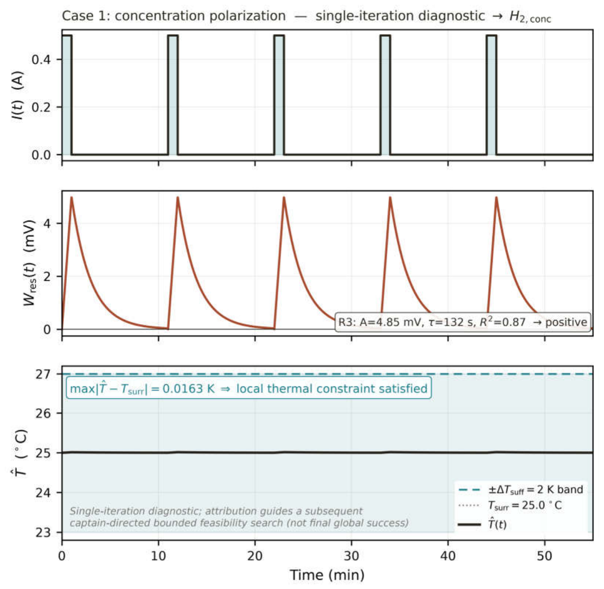
6.2. Case 2 — Plateau-Geometry Tilt (R6 → H2,Phase)
Case 2 (config case2_phase.yaml, seed 20260724) injects a plateau-geometry tilt: the pulse-plateau residual amplitude rises across composition and persists through rest as a structural offset, on the same 0.5 A/60 s/600 s protocol. The mechanism to be recognised is H2,phase.
Expected reasoning: R3 negative (no clean positive rest relaxation); R6 positive (upward plateau tilt across composition, high linearity); R8 negative; local thermal constraint satisfied.
Generator output (authoritative; results/case2):
- R3 = negative; the rest-relaxation fit is not a positive monotonic decay (end-of-rest amplitude not positive), so H2,conc is not indicated.
- R6 = positive; the pulse-plateau amplitude tilts upward across composition with slope +327.8 mV per unit composition and near-perfect linearity (R2 ≈ 1.00), well beyond the 5 mV-per-unit threshold.
- R8 = negative; the highest-stress residual is positive, so the thermal signature is absent.
- Local thermal constraint = satisfied: max|T̂ — T_surr| = 0.0168 K, within the 2 K band (one local evaluation, not a global verdict).
- Diagnostic attribution: H2,phase at moderate confidence (single positive rule, R6). The thermal constraint is satisfied at this point and R6 guides a bounded feasibility search for a phase-morphology-consistent parameter set.
Figure 6.2 shows the Case 2 channels: current drive, the tilted W_res(t) plateau signature, and the temperature against the 2 K band.
Three-panel synthetic Case 2 figure. (a) GITT current drive. (b) Injected plateau-geometry tilt in reaction-work residual W_res(t) read by rule R6 (slope +327.8 mV per unit composition, R2 approx 1.00). (c) Simulated cell temperature against the 2 K local thermal band, max|T_hat - T_surr| = 0.0168 K: local thermal constraint satisfied. Single-iteration diagnostic whose H2,phase attribution guides a captain-directed bounded feasibility search, not a final global success.
Figure 6.
2. Synthetic BMS-like Case 2 (config case2_phase.yaml, seed 20260724). (a) GITT current drive; (b) injected plateau-geometry tilt in W_res(t), detected by R6 (slope +327.8 mV per unit composition, R2≈1.00); (c) simulated temperature against the 2 K local thermal band, max|T̂−T_surr| = 0.0168 K (local thermal constraint satisfied). Diagnostic attribution H2,phase: a single-iteration diagnostic evaluation whose attribution guides a subsequent captain-directed bounded feasibility search, not a final global success. Synthetic methodological case, not measured data; regenerate from the reproducibility package.
Figure 6.
2. Synthetic BMS-like Case 2 (config case2_phase.yaml, seed 20260724). (a) GITT current drive; (b) injected plateau-geometry tilt in W_res(t), detected by R6 (slope +327.8 mV per unit composition, R2≈1.00); (c) simulated temperature against the 2 K local thermal band, max|T̂−T_surr| = 0.0168 K (local thermal constraint satisfied). Diagnostic attribution H2,phase: a single-iteration diagnostic evaluation whose attribution guides a subsequent captain-directed bounded feasibility search, not a final global success. Synthetic methodological case, not measured data; regenerate from the reproducibility package.
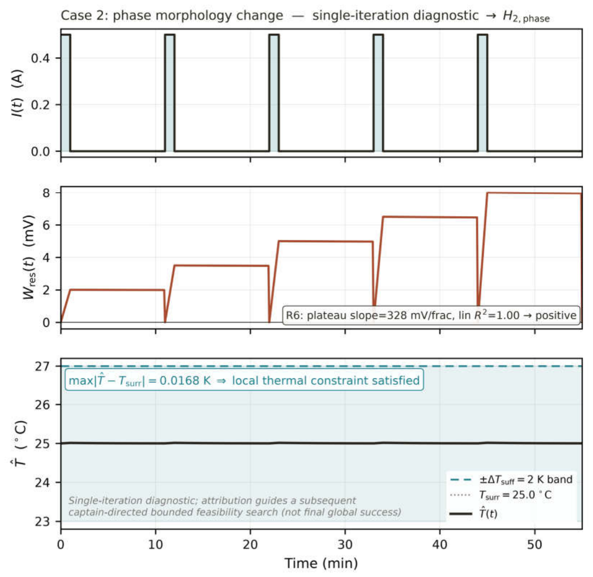
6.3. Case 3 — Negative Sign-and-Decay Thermal Residual (R8 → H2,Thermal)
Case 3 (config case3_thermal.yaml, seed 20260725) injects a thermal-feedback residual: a negative sign-and-decay signature under higher-stress pulses (2.3 A, 120 s pulses, weak cooling h_cA_h = 0.08 W/K). The mechanism to be recognised is H2,thermal, whose distinguishing feature is the negative residual sign.
Expected reasoning: R3 negative (residual is negative, disqualified by R3’s positive-sign requirement); R6 negative (negative slope); R8 positive (negative residual with monotonic magnitude decay on the thermal timescale); thermal excursion still within the 2 K band under this protocol.
Generator output (authoritative; results/case3):
- R3 = negative; the fitted rest amplitude is negative, rejected by R3’s positive-sign requirement, so R3 does not misattribute the thermal signature as concentration polarization.
- R6 = negative; the plateau slope is negative, rejected by R6’s positive-tilt requirement.
- R8 = positive; the highest-stress rest residual starts at −10.9 mV (negative, beyond the noise floor) and decays monotonically in magnitude on the thermal timescale — the distinguishing thermal signature.
- Local thermal constraint = satisfied: max|T̂ — T_surr| = 0.7305 K, within the 2 K band for this GITT pulse-and-rest protocol. (This is a single local evaluation for this protocol and must not be conflated with the natural-convection (h_c = 15 W·m−2·K−1) curve of the 1C-continuous discharge inFigure 1.3, whose local thermal constraint is violated (while higher-h_c curves in the same figure satisfy it))
- Diagnostic attribution: H2,thermal at moderate confidence (single positive rule, R8). The thermal constraint is satisfied under this protocol and R8 initialises a bounded feasibility search; a global outcome would follow from captain-directed reruns, including conditions that stress the thermal constraint more strongly.
Figure 6.3 shows the Case 3 channels: the higher-stress current drive, the negative W_res(t) sign-and-decay residual read by R8, and the temperature against the 2 K band.
Three-panel synthetic Case 3 figure. (a) Higher-stress GITT current drive (2.3 A, 120 s pulses). (b) Negative sign-and-decay reaction-work residual W_res(t), start -10.9 mV, read by rule R8. (c) Simulated cell temperature against the 2 K local thermal band, max|T_hat - T_surr| = 0.7305 K: local thermal constraint satisfied under this GITT protocol, distinct from the 1C-continuous Figure 1.3 whose local thermal constraint is violated. Single-iteration diagnostic whose H2,thermal attribution initialises a captain-directed bounded feasibility search, not a final global success.
Figure 6.
3. Synthetic BMS-like Case 3 (config case3_thermal.yaml, seed 20260725). (a) higher-stress GITT current drive (2.3 A, 120 s pulses, h_cA_h = 0.08 W/K); (b) negative sign-and-decay residual W_res(t) (start −10.9 mV) detected by R8; (c) simulated temperature against the 2 K local thermal band, max|T̂−T_surr| = 0.7305 K (local thermal constraint satisfied under this GITT protocol; distinct from the natural-convection (h_c = 15 W·m−2·K−1) curve of the 1C-continuousFigure 1.3, whose local thermal constraint is violated.
Figure 6.
3. Synthetic BMS-like Case 3 (config case3_thermal.yaml, seed 20260725). (a) higher-stress GITT current drive (2.3 A, 120 s pulses, h_cA_h = 0.08 W/K); (b) negative sign-and-decay residual W_res(t) (start −10.9 mV) detected by R8; (c) simulated temperature against the 2 K local thermal band, max|T̂−T_surr| = 0.7305 K (local thermal constraint satisfied under this GITT protocol; distinct from the natural-convection (h_c = 15 W·m−2·K−1) curve of the 1C-continuousFigure 1.3, whose local thermal constraint is violated.
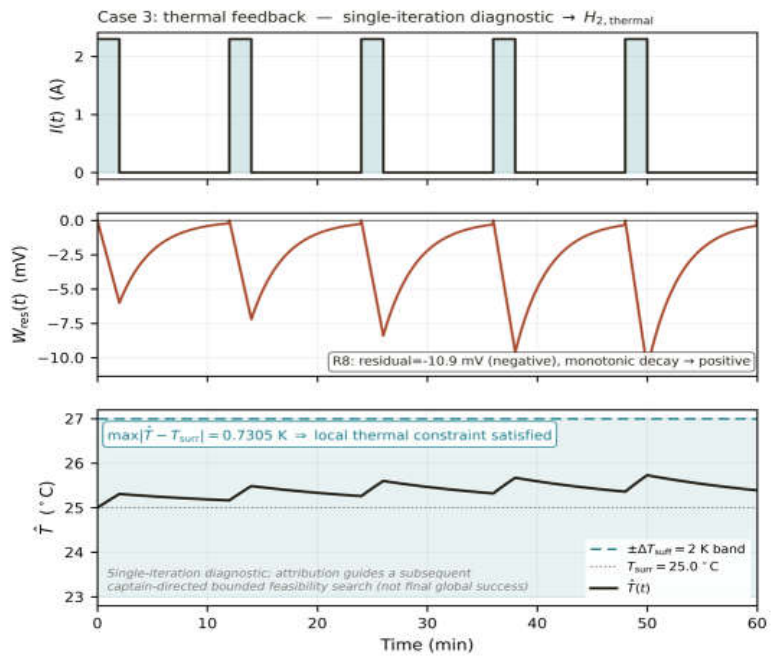
6.4. Case 4 — Negative Control: No Injected Signature (H0, Insufficient Evidence)
Case 4 (config case4_null.yaml, seed 20260726) is the negative control: no mechanism signature is injected, only measurement noise, on the baseline 0.5 A/60 s/600 s protocol. It tests whether the framework recognises insufficient evidence and refuses to over-attribute.
Generator output (authoritative; results/case4):
- R3 = negative; the residual is within the noise floor with no positive monotonic relaxation.
- R6 = negative; no plateau tilt above threshold.
- R8 = negative; the highest-stress residual is within σ of zero (null-consistent), so no thermal signature.
- Local thermal constraint = satisfied: max|T̂ — T_surr| = 0.0153 K, within the 2 K band. The thermal constraint is satisfied, yet no mechanism attribution is licensed — the local constraint state and the evidentiary state are distinct.
- Global outcome = indeterminate (H0). No R-rule returns a positive mechanism signature and the residual lies within the noise floor, so the framework declines to attribute any H_2 member and instead requests a more informative operating condition (for example a higher-rate or multi-ambient scan) rather than forcing a conclusion. The thermal constraint is satisfied; observability is insufficient. This is the indeterminate outcome of §2.6.1, not a global failure.
This negative control is the study’s central falsifiability demonstration: a framework that could not return “insufficient evidence” would over-fit noise. Case 4 shows the reasoning recognising the absence of signal and refusing attribution, while still reporting an honest local-thermal-constraint-satisfied result.
Figure 6.4 shows the Case 4 channels: current drive, the flat (noise-only) W_res(t), and the temperature against the 2 K band; all rules negative → H0.
Three-panel synthetic Case 4 negative-control figure. (a) Baseline GITT current drive. (b) Flat noise-only reaction-work residual W_res(t), all rules negative. (c) Simulated cell temperature within the 2 K local thermal band, max|T_hat - T_surr| = 0.0153 K: local thermal constraint satisfied. Global outcome indeterminate (H0): no attribution licensed; the framework requests a more informative operating condition rather than forcing a conclusion.
Figure 6.
4. Synthetic BMS-like Case 4 negative control (config case4_null.yaml, seed 20260726). (a) baseline GITT current drive; (b) noise-only W_res(t), all rules negative; (c) simulated temperature within the 2 K local thermal band, max|T̂−T_surr| = 0.0153 K (local thermal constraint satisfied). Global outcome indeterminate (H0): no attribution licensed — the framework declines to attribute a mechanism and instead requests a more informative operating condition rather than forcing a conclusion. Synthetic methodological case, not measured data.
Figure 6.
4. Synthetic BMS-like Case 4 negative control (config case4_null.yaml, seed 20260726). (a) baseline GITT current drive; (b) noise-only W_res(t), all rules negative; (c) simulated temperature within the 2 K local thermal band, max|T̂−T_surr| = 0.0153 K (local thermal constraint satisfied). Global outcome indeterminate (H0): no attribution licensed — the framework declines to attribute a mechanism and instead requests a more informative operating condition rather than forcing a conclusion. Synthetic methodological case, not measured data.
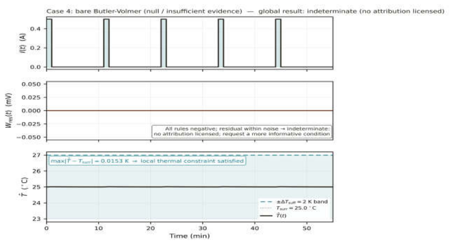
6.5. Summary of the Illustrative Example
Table 6.
1. Per-case diagnostic attribution and local thermal-constraint state across the four synthetic single-iteration case studies (authoritative generator outputs). Case 4 is the indeterminate outcome: the local thermal constraint is satisfied but no attribution is licensed.
Table 6.
1. Per-case diagnostic attribution and local thermal-constraint state across the four synthetic single-iteration case studies (authoritative generator outputs). Case 4 is the indeterminate outcome: the local thermal constraint is satisfied but no attribution is licensed.
| Case | Injected signature | Positive rule | Attribution | Confidence |
| 1 | concentration-polarization memory | R3 | H2,conc | moderate |
| 2 | plateau-geometry tilt | R6 | H2,phase | moderate |
| 3 | negative sign-and-decay (thermal) | R8 | H2,thermal | moderate |
| 4 | none (noise only) | — | H0 (indeterminate; no attribution licensed) | n/a (indeterminate) |
Across the four single-iteration cases the diagnostic reasoning forms a clean diagonal, each case being one constraint evaluation that would seed a bounded feasibility search rather than a terminal classification:
- exactly one positive rule fires per mechanism case — R3 for concentration polarization (Case 1), R6 for phase morphology (Case 2), R8 for thermal feedback (Case 3) — and none fires for the null (Case 4);
- each of the three implemented rules (R3, R6, R8) is affirmative on exactly the case whose signature it targets and negative elsewhere, showing cross-mechanism discrimination without misattribution;
- the local thermal-constraint instrument returns an honest verdict in every case, and Case 4 separates thermal-envelope status (satisfied) from evidentiary sufficiency (not satisfied);
- and the negative control (Case 4) exercises the framework’s refusal to over-attribute, returning H0/insufficient evidence rather than forcing a mechanism.
What these cases do not demonstrate. They are synthetic and carry no claim of experimental validation, real onboard battery-management-system performance, proprietary data, parameter estimation, or quantitative generalization to physical cells. Only the three rules decidable from a single GITT record (R3, R6, R8) are executed; the remaining R-rules (memory and magnitude R1–R2, composition asymmetry R4, rate-scan character and asymmetry R5/R7, ambient-scan and thermal-correlation R9/R10) require multi-rate or multi-ambient data that a single synthetic record does not contain, and are therefore not executed and not claimed to have been tested.
On reproducibility. Every number in this section is the deterministic output of the accompanying generator at the stated configuration and seed; re-running the package reproduces the CSV time series, JSON summaries, and these figures, and the automated test suite checks the injected-signature recovery and the sufficiency and insufficient-evidence logic.
7. Discussion
7.1. Comparison with Existing Approaches to LFP Modeling
The present framework belongs to a different program from most published LFP single-particle modeling work. The dominant tradition — the Newman pseudo-2D framework and its single-particle simplifications [17,18,19] — is forward: assume the electrochemical PDEs and constitutive relations, solve for given the current schedule,
and validate against experimental terminal measurements. Extensions into
phase-field territory [1,16,20] add spatially-resolved
coherency-strain and Cahn–Hilliard morphology dynamics, and coupled
electrothermal implementations [11]
integrate the resulting PDEs numerically in COMSOL to produce traces for arbitrary drive
cycles. The present framework’s inverse-attribution program is complementary
rather than competing: rather than solve the coupled PDEs and validate the
trajectory, it reads the measured at the symmetry point where
the bivariate kernel decouples, and asks which of an enumerated set of
non-Butler–Volmer mechanisms is responsible for the observed deviation from the
bare kinetic prediction. The forward and inverse programs consume the same
experimental observables but arrive at different deliverables: the forward
program produces a validated coupled-PDE model whose parameters can be
interrogated for physical meaning; the inverse program produces a
per-observation-instant mechanism verdict with an explicit confidence grade and
a local thermal-constraint flag.
The methodological posture of the author’s parallel program — that robust full-physics models of the coupled response of an LFP cell do not exist without stark structural
approximations, and that data-discovered effective theories are the principled
response, articulated in an in-preparation review paper on the LFP modeling
landscape — is the sibling program to the present paper’s approach. The review
positions PCA-then-regression as an information-flow realization of Mahler’s
effective-theory program; the present paper positions the R-rule discrimination
logic as a Mahler-grounded inverse-attribution program on the symmetry-point
observable. Both share the refusal to force a single closed-form microscopic
model onto observations that cannot be reproduced dot-by-dot by any lumped
abstraction. The two papers are complementary contributions from the same
author’s program and should be read together for readers interested in the
underlying methodological stance.
What the present framework does not claim, and what forward-simulation frameworks legitimately do, is a validated map from constitutive parameters to observable trajectories. The framework does not fit , , phase-field parameters, or thermal-feedback activation energies.
It does not produce a model that can be interrogated for the numerical value of
any of these. It produces a mechanism verdict on the enumerated hypothesis
space and a local thermal-constraint flag.
7.1.1. Illustrative BMS Integration
To make concrete what the reasoning would consume in an onboard setting, consider—illustratively, not as a deployed or validated system—how the channels a conventional LFP-pack battery-management system already records map onto the framework’s inputs. This is a conceptual mapping on synthetic BMS-like signals; no onboard implementation, real-pack record, or performance benchmark is claimed. In the same spirit, the energy-closure gate (Eq. (15)) makes admissibility a prerequisite for interpretation: a candidate that does not close energetically is rejected as a computational/model inconsistency before its thermal margin or mechanism attribution is read.
Inputs the framework reads. The framework’s on-board instantiation consumes the signals a conventional LFP-pack BMS already measures: per-cell terminal voltage , pack current , and — where the pack is instrumented for it — surface
temperature . No additional sensor is required. The composition variable is taken from the existing coulomb-counting state-of-charge
estimator; the elected curve and the standard potential are stored as calibration constants in read-only memory per cell
chemistry.
When the framework fires. The attribution logic evaluates at each pack rest step — charge tail, drive-cycle regen tail, parking event, grid-storage cycle boundary — of duration s during which the running coulomb count places one or more cells
inside a captain-defined composition window around the symmetry point ( , with set to preserve the bivariate-kernel decoupling per §1.4.4).
Between rest steps the framework is idle; it does not require continuous
coupled-PDE integration.
What the on-board logic block computes. At each firing event, four quantities are produced:
- The lumped simulated temperature from Eq. (13) integrated over the rolling window using the elected and stored thermal parameters . One ODE integration per rest step.
- The voltage-derived reaction work at the anchor, (in absorbed voltage units per §1.4.3), evaluated at each crossing within the window.
- The R-rule battery of §5.1–§5.3 evaluated on the signature at the anchor: R3 relaxation timescale and amplitude sign, R6 plateau tilt sign, R8 sign-and-decay envelope, with sign discipline as specified in §5. Each R-rule returns positive/negative/inconclusive with its associated confidence grade.
- The local thermal-constraint flag on against the captain-specified band : sufficient, or one of the three insufficient sub-cases (systematic offset, current-coupled, magnitude excursion) per §5.4.2.
The compute footprint is one ODE integration and a small decision tree of R-rule evaluations per firing event. No live parameter fitting is performed; no coupled PDE is solved. This is well inside the budget of embedded automotive-class controllers.
What the BMS emits. The framework produces a structured joint report at each firing event: {mechanism ∈ [H2,conc | H2,phase | H2,thermal | inconclusive], sufficiency ∈ [sufficient | insufficient-{offset, current, magnitude}], confidence grade}. This report is the framework’s contribution to the vehicle control stack; how the vehicle acts on it is a separable design choice for the integrator.
How the vehicle side changes. For concreteness, three example branches on the joint report illustrate what mechanism attribution enables that terminal-voltage thresholding alone does not:
- H2,conc-dominant, sufficient. The concentration-polarization signature at the anchor flags solid-state diffusion as the rate-limiter. The BMS derates the fast-charge current envelope; further increase will not translate to faster charging and is likely to accelerate anode-side plating on graphite. Conventional BMS logic derates on measured voltage crossing a threshold; the framework’s verdict identifies why the voltage response is what it is and specifies that rest, not cooling, is the release mechanism.
- H2,phase-dominant, sufficient. The coherency-strain plateau-tilt signature is logged as a state-of-health input distinct from the conventional capacity-fade/resistance-growth SoH metrics. It flags mechanical fatigue of individual particles — a degradation channel whose accumulation is currently invisible to pack-level capacity tracking. The pack’s cycle-life warranty model receives this as a separate input dimension.
- H2,thermal-dominant, or the local thermal constraint is violated. The thermal-feedback signature, or a violated local thermal constraint, triggers the energy-closure admissibility check and a bounded cooling/operating-condition search rather than an immediate control action: the BMS flags the operating point for captain review and, where a realizable cooling or duty-cycle adjustment can return the cell inside the 2 K band, recommends it. A single local-constraint violation is treated as one diagnostic flag, not as a global failure, and does not by itself command an automatic derate.
Explicit local-constraint guarantee. Every attribution emitted to the vehicle carries the local thermal-constraint flag. When that local thermal constraint is violated in any of the three sub-cases, the mechanism attribution is downgraded to advisory per §5.4.2 — recorded in the vehicle log for offline health analysis but not permitted to trigger control-loop action. This is the substance of the local-constraint guarantee: the framework refuses to act on its own mechanism attribution when its own instrument reports that the operating point violates the local thermal constraint, deferring instead to a captain-directed feasibility check.
What the framework does not do on the BMS. The framework does not fit or live; does not require a coupled-PDE forward model on-chip; does
not replace the state-of-charge estimator; does not require recalibration
outside the elected OCV curve; does not extrapolate beyond the
local-thermal-constraint band without a captain-directed rerun.
This illustrative integration is offered as a target for follow-on validation on experimental datasets and, subsequently, on instrumented BMS testbeds. Whether
the R-rule sign discipline calibrated on the illustrative-example synthesis
(§6) survives translation to real drive-cycle records, and whether the local
thermal-constraint band can be tuned to give useful discrimination without excessive
advisory-downgrade events, are the primary questions any BMS-integration
program would need to answer before onboard deployment.
7.1.2. Positioning Relative to AI-Assisted and Simulation-Based Diagnosis
Several recent programs share individual components with the present framework. In the battery domain, model-based diagnosis on simulated cells derives physics-model admissibility regions and treats overlapping cases as ambiguous outcomes [21], and an LLM agent has been placed in a closed loop with a battery simulator to reason over simulated battery physics and revise hypotheses iteratively [22]. In process engineering, interpretable LLM diagnosis has been applied to simulator-generated chemical-process signals over a bounded, curated hypothesis space [23]. These works establish that reasoning over synthetic physics-based signals, physics-grounded hypothesis constraints, and interpretable diagnostic output are each precedented.
The present framework is not distinguished by any one of these ingredients but by how they are composed under human command. Its contribution is the governed composition of independent synthetic evidence, a physics/energy-closure admissibility gate, transparent named heuristic rules, human command authority over a bounded rerun, and a tri-valued (feasible/infeasible/indeterminate) decision-support outcome. Where the closest precedents either replace the human with an autonomous agent [22], omit an explicit energy-closure admissibility gate and named rule catalogue [21,23], or keep the diagnostic verdict binary, the framework retains a human captain as the controller of the rerun loop, gates every candidate on energy closure before interpretation, and preserves indeterminate as a legitimate reported outcome. The synthetic signals are held independent of the reasoning kernel and the controlled cases are methodological demonstrations rather than performance claims. No claim of priority is made for any individual element.
7.2. Open Questions on Transferability Beyond LFP
The framework’s derivational grounding depends on two properties of the LFP electrochemical system that are not universal: the regular-solution symmetry at that decouples the
bivariate kernel (§1.4.4), and the small reversible entropic contribution over the operating range
that permits its being dropped from the lumped enthalpy balance (§1.4.7).
Transferring the framework to other intercalation chemistries — NMC, NCA, LMO,
or the emerging sodium-ion analogs — requires an audit of these two dependencies
for each candidate.
The symmetry-point identity is the most restrictive of the two. Regular-solution symmetry at half-filling is a specific consequence of the LFP two-phase thermodynamics and its narrow miscibility gap; NMC and NCA are single-phase solid solutions across most of the operating range and do not exhibit a symmetry point where the bivariate kernel decouples by construction. For these chemistries, the framework’s Mahler-grounded direct observability of at does not carry over, and either an alternative reference point
must be identified from first principles or the framework must fall back on a
symmetry-broken form of the discrimination heuristic that estimates from off-symmetry-point calibration. Both are open questions the
present paper does not resolve.
The local thermal-constraint instrument transfers more directly. Eq. (14) is a per-iteration constraint on |T̂(t) — T_surr| against a captain-declared band; in any coupled model it supplies one constraint margin and flag that the feasibility search of §2.6.1 balances against the kinetic and mass-transfer constraints, rather than a standalone accept/reject test.
A half-reaction analogy (used only as conceptual explanation). Just as two individually balanced half-reactions must still satisfy joint charge and mass conservation when combined into a full cell reaction, the individually plausible thermal, kinetic, and mass-transfer submodels here must satisfy joint conservation and closure when coupled. A submodel that looks admissible in isolation can violate the joint balance; the feasibility search resolves this by revising coefficients and parameters only within their declared physical bounds, never by arbitrary tuning to force closure.
Parameter inference versus control design. The coefficient h_c plays two distinct roles that the paper keeps separate. In a diagnostic evaluation it is an inferred heat-transfer coefficient describing the cell as observed; in a feasibility search it is a candidate cooling or control requirement — a demand that a realizable design action (a fan, a coolant loop, a duty-cycle limit) would have to meet. The search does not ‘change’ a physical coefficient by fiat: an update to h_c is admissible only as either a re-inference justified by the data or a control-design target that a stated, realizable actuator could deliver within practical limits. A solution that would require an impractical h_c is reported as infeasible, not as a free parameter change.
The R-rule discrimination logic — R3 relaxation timescales, R6 plateau tilts, R8 sign-and-decay, R11 sweeps — is chemistry-neutral in its structural form but
chemistry-dependent in its threshold calibration. The illustrative example’s
sign discipline (R3 requires positive amplitude, R6 requires positive slope, R8
requires negative end amplitude) reflects LFP-specific expectations about how
each mechanism perturbs relative to bare Butler–Volmer, and would need re-examination for
chemistries with different phase-transition and diffusion physics. Whether the
R-rule framework survives translation to non-symmetry-point observables in
NMC/NCA is the primary open question for cross-chemistry transferability.
7.3. Methodological Reflections on the AI-Captain Partnership Beyond the Case Study
The paper’s principal contribution is methodological rather than electrochemical: a demonstration that, in this case, human–AI collaboration on an extended technical problem can produce a well-scoped, falsifiable framework when specific disciplinary structures are enforced. The LFP application is the diagnostic test bed; the transferable claim is the collaboration pattern itself. Three reflections merit separation from the case study.
First, the role asymmetry between captain and expert system is load-bearing rather than incidental.Section 2 documents four observable failure modes — confabulation of derivational content, silent drift in commitments across long sessions, over-specification of scope, and premature closure on captain-uncertain claims — and the captain-mediated recovery for each. The asymmetry is not that the captain is smarter or the AI faster; it is that the captain owns authority for scope and commitment while the AI owns structural bookkeeping under captain-declared constraints. This division survives beyond LFP for any partially closed theory whose domain is opaque enough that the AI cannot self-audit its derivations yet structured enough that it can carry the bookkeeping burden that would otherwise cost the captain hours per session.
Second, the structured handoff document as an anti-hallucination scaffold is the pattern’s most transferable artifact. §2.3 identifies four mechanisms by which it constrains the expert system in a fresh thread: naming captain-authorized commitments, listing scope corrections and their justifications, recording prior-thread failure modes, and declaring the open questions the thread may work on. All four are chemistry- and application-neutral. The handoff is not a summary but a constraint document that reshapes the expert system’s decision boundary — directly available for adoption in long-running engineering, regulatory, protocol-development, or academic-research work beyond electrochemistry.
Third, the failure-mode catalog (§2.4) is the primary reviewer-facing evidence that the pattern is disciplined rather than ad hoc: each failure mode is named, its diagnostic signature characterized, and its captain-mediated recovery documented. It is the pattern most vulnerable to being read as anecdotal, and the most directly extensible — new failure modes can be added and recovery patterns refined as collaborations accumulate a track record. The catalog is not claimed exhaustive; it is claimed falsifiable and extendable, offered as an initial baseline for a discipline that lacks one.
These reflections do not resolve whether AI-assisted reasoning in partially closed physical theories is safe for consequential engineering decisions; that requires an accumulated track record across many collaborations in domains where ground truth eventually becomes available. The present paper offers one such record, honestly documented, in a domain where the LFP literature provides enough external reference to check the framework’s structural claims against established physics. Whether the pattern generalizes is a matter for subsequent papers and collaborations, not the present case study.
8. Conclusions
This methodological case study demonstrates how a human-guided AI expert system applies heuristic reasoning to synthetic signals representative of those available from an onboard battery-management system. The LiFePO4 single-particle model and its cited modeling relationships provide the analytical scaffolding; the contribution is the human–AI reasoning pattern and its evaluation on transparency, consistency, traceability, falsifiability, and recognition of insufficient evidence. The framework also enforces an explicit ordering — energy-closure admissibility, then the local 2σ/2 K thermal constraint, then coupled feasibility, then captain-directed bounded rerun — keeping numerical consistency logically prior to physical interpretation.
The four synthetic case studies of Section 6 demonstrate the reasoning end-to-end on reproducible, fully owned signals: R3, R6, and R8 each fire on exactly the mechanism case they target (Cases 1–3, attributing H2,conc, H2,phase, and H2,thermal respectively), and the negative-control Case 4 returns the indeterminate outcome (H0) rather than over-attributing noise. In all four cases the local thermal constraint is satisfied under the 2 K test; each case is a single iteration of the captain-directed feasibility search, and Case 4 is the indeterminate outcome, keeping the satisfied local thermal constraint distinct from the unlicensed attribution and requesting a more informative condition.
The paper’s principal contribution is methodological: an evaluation of how a human-guided AI expert system reasons over synthetic BMS-like signals — explicit role asymmetry between human authority and AI structural bookkeeping, the structured handoff document as an anti-hallucination scaffold, an observable failure-mode catalog with captain-mediated recovery, and a reasoning pattern that recognises when the evidence is insufficient. The synthetic case studies are the vehicle for that evaluation, not an empirical validation.
What this paper does not do is fit constitutive parameters, reconstruct microscopic heat–work partitions, claim experimental validation, use real onboard battery-management records or proprietary data, or assert quantitative generalization to physical cells. The single externally-sourced input is a cited, digitized approximation of the Forgez (2010) entropic curve, used only as declared modeling structure. Cited literature relationships are background modeling structure, not owned observations.
Supplementary Materials
The following supporting information can be downloaded at the website of this paper posted on Preprints.org. The following supporting information is uploaded directly with this article for peer review: Supplementary Materials S1: Paper A Framework—Real-Data User’s Manual — the full operational manual for applying the framework to real measured data. Supplementary Material S2: Paper A Reproducibility Package v1.0.0 — the complete software/supplementary archive (Python source, case configuration files, synthetic data and machine-readable outputs, figures, automated test suite, energy-closure audit, and metadata/licenses). Both S1 and S2 are uploaded directly with the manuscript for peer review. A permanent repository DOI may be added at a later stage but is not required for peer review.
Author Contributions
Conceptualization, Roger Painter and Irucka Embry; Methodology, Ranganathan Parthasarathy and Roger Painter; Formal analysis, Roger Painter; Investigation, Roger Painter; Resources, Lin Li, Lonnie Sharpe and S. Keith Hargrove; Data curation, Roger Painter; Writing—original draft preparation, Roger Painter and Irucka Embry; Writing—review and editing, Ranganathan Parthasarathy, Roger Painter and Irucka Embry; Visualization, Roger Painter; Supervision, Lin Li, Lonnie Sharpe and S. Keith Hargrove; Project administration, Lin Li, Lonnie Sharpe and S. Keith Hargrove; Funding acquisition, Lin Li, Lonnie Sharpe and S. Keith Hargrove. All authors have read and agreed to the published version of the manuscript.
Funding
Funding was provided by the Massie Chair of Excellence at Tennessee State University and the Office of the Dean of the College of Engineering at Tennessee State University.
Institutional Review Board Statement
Not applicable.
Informed Consent Statement
Not applicable.
Data and Software Availability
All signals in this study are synthetic and are produced by the reproducibility package uploaded directly with this paper as Supplementary Material S2 (Paper A Reproducibility Package v1.0.0). S2 contains the signal generator, the four case configuration files with fixed random seeds, the heuristic-evaluation code, the machine-readable outputs (CSV time series and JSON summaries) for each case, the figure-generation scripts, the seven manuscript figures, and an automated test suite; running it regenerates every Section 6 number and figure deterministically. The only externally-sourced input is a digitized approximation (≈±0.05 mV/K) of the entropic coefficient dU/dT from Forgez et al. (2010) Fig. 4a, included as a cited modeling input and clearly labelled as a figure reconstruction rather than a vendor numeric table. No proprietary, experimental, or commercial battery-management-system data are used or distributed. S2 additionally includes the machine-readable Figure 1.3 energy-closure audit (JSON summary and the per-curve sweep CSV) and the tested energy-audit script that recomputes the integrated , , , , Δ and the closure residual reported here; the audit verifies the numerical
solution’s internal energy consistency (solver/model closure), not experimental
or hardware validity. All synthetic signals, configuration files, code,
results, figures, tests, and the energy audit are included in S2; the companion
operational manual for applying the framework to real measured data is provided
as Supplementary Material S1 (see the Supplementary
Materials statement above and
Appendix A). Both S1 and S2 are uploaded directly with the manuscript for peer
review, so the supporting materials are available to reviewers at submission; a
permanent repository DOI may be added at a later stage but is not required for
peer review. The original contributions presented in this study are included in
the article and its Supplementary
Materials; further inquiries
can be directed to the corresponding author.
Conflicts of Interest
Irucka Embry is the owner of EcoC2S. The paper reflects the views of the authors and not the company.
Appendix A
Real-Data Framework User Manual. The full operational manual for applying this framework to real measured battery data is provided as Supplementary Material S1 (Paper A Framework—Real-Data User’s Manual) rather than reproduced in full here, to keep the article self-contained. The manual documents the operational scope of the framework: real-data readiness criteria; mapping of measured channels (current, terminal voltage, and temperature records) onto the framework’s inputs; the energy-closure admissibility check; the iterative-feasibility procedure and its captain-directed bounded search; and the records and governance practices (configuration history, decision record, and audit logs) that support artifact-level reproducibility.
The manual describes a methodological procedure only. It does not claim turnkey compatibility with any real battery-management system, and it does not assert safety, control, or actuation authority over any physical cell, pack, or vehicle. Any application to hardware remains subject to independent validation outside the scope of this article.
Appendix B
Supporting methodological material and Mahler-equation provenance. This appendix records the provenance of the thermodynamic structure used in Section 1.4. The framework’s bivariate first-law grounding is drawn from the quantum-thermodynamic treatment of Gemmer, Michel, and Mahler [9]; the relationships below identify the specific results in that source on which the derivation in §1.4 depends. They are cited source relationships, reproduced here for traceability of the derivation; no claim of reproduction rights or copyright permission is made or implied.
B.1. Mahler bivariate first law — source relationships. The bivariate first-law structure adopted in §1.4.1 corresponds to Eqs. (4.75)–(4.86) of Mahler [9] §4.3, with the generalized non-thermal control parameter introduced in Definition 4.23, Eq. (4.91) (with the explicit qualifier that the control parameter need not be mechanical), and the classical limit established via Eq. (4.74). The specific results relied upon are Eqs. 4.74, 4.75, 4.80, 4.85, 4.86, 4.91, 4.92, 4.97, and 4.102, together with Definitions 4.12, 4.14, 4.16, 4.23, 4.24, and 4.25. These are the source relationships underlying the bivariate kernel and its symmetry-point specialization; the framework’s own numbered equations (1)–(23) in the body are distinct from this source numbering.
B.2. Classical-limit refinement. As noted in §1.4.2, the LFP particle is a composite host lattice rather than a point particle; the classical-limit criterion of Mahler [9] is applied to the framework’s domain of application accordingly, and the bivariate structure is used in its classical or quasi-classical sense throughout. This refinement is the only adaptation of the source relationships required for the electrochemical instance treated here.
Appendix C
Reproducibility package inventory. The case study’s artifact-level reproducibility claim (§2.5 and §3.5) rests on the software artifacts of the reproducibility package, provided in full as Supplementary Material S2 (Paper A Reproducibility Package v1.0.0) and uploaded directly with the manuscript for peer review. S2 contains, exactly:
- Source code (bms_synth/) — the synthetic-signal generator and framework logic (generator, OCV model, signatures, heuristics, case definitions, configuration handling, energy audit, the Figure 1.3 sweep, export, and package entry points).
- Configuration files (configs/) — four YAML case configurations (case1_conc, case2_phase, case3_thermal, case4_null) with fixed random seeds.
- Generated case outputs (results/) — per-case machine-readable outputs (CSV time series and JSON summaries) for the four cases.
- Figure 1.3 h_c sweep and energy-closure audit — the sweep outputs (fig13_hc_sweep.json, fig13_hc_sweep.csv) and the energy-closure audit (fig13_energy_closure.json, fig13_energy_closure.csv), together with the run_energy_audit.py driver.
- Figure-generation scripts and figures — make_figures.py, make_case_figures.py, and make_fig13_sweep.py, and the seven manuscript figures rendered in both PNG and TIFF (figures/).
- Automated test suite (tests/) — the 68-test pytest suite covering determinism, units/ranges, signature recovery, sufficiency, attribution, protocol timing, configuration export, the Figure 1.3 sweep, and the energy audit.
- Metadata, provenance, and licensing — README.md, LIMITATIONS.md, manifest.json, CITATION.cff, AUTHORS.md, the change log (CHANGELOG.md), the checksums file (SHA256SUMS.txt), the license files (LICENSE-MIT, LICENSE-CC-BY-4.0, LICENSES.md), the digitized Forgez et al. (2010) Fig. 4a dU/dT input with its data/README.md provenance note, and requirements.txt.
- Operational manual copy (docs/) — a copy of Supplementary Material S1 (the Real-Data User’s Manual).
S2 is uploaded directly with the manuscript for peer review; no repository DOI is assigned at submission, and a permanent repository DOI may be added at a later stage. The package documents artifact-level reproducibility through the configuration files, fixed seeds, generated outputs, checksums, and automated tests above; it does not include, and this article does not promise, raw human—AI conversation transcripts or confidential internal development records.
References
- Zeng, Y.; Bazant, M.Z. Phase Separation Dynamics in Isotropic Ion-Intercalation Particles. SIAM J. Appl. Math. 2014, 74, 980–1004. [Google Scholar] [CrossRef]
- Bazant, M.Z. Theory of Chemical Kinetics and Charge Transfer Based on Nonequilibrium Thermodynamics. Acc. Chem. Res. 2013, 46, 1144–1160. [Google Scholar] [CrossRef] [PubMed]
- Venkatasubramanian, V.; Rengaswamy, R.; Kavuri, S.N. A Review of Process Fault Detection and Diagnosis Part II: Qualitative Models and Search Strategies. Comput. Chem. Eng. 2003, 27, 313–326. [Google Scholar] [CrossRef]
- Kuipers, B. Qualitative Simulation. Artif. Intell. 1986, 29, 289–338. [Google Scholar] [CrossRef]
- de Kleer, J.; Williams, B.C. Diagnosing Multiple Faults. Artif. Intell. 1987, 32, 97–130. [Google Scholar] [CrossRef]
- Garrido-Merchán, E.C.; Puente, C. GOFAI Meets Generative AI: Development of Expert Systems by Means of Large Language Models. arXiv 2025, arXiv:2507.13550. [Google Scholar] [CrossRef]
- Sun, B.; Zhao, X.; He, X.; Ruan, H.; Zhu, Z.; Zhou, X. Virtual Battery Pack-Based Battery Management System Testing Framework. Energies 2023, 16, 680. [Google Scholar] [CrossRef]
- Kaufmann, D.; Kozovsky, M.; Wotawa, F. Simulation-Based Diagnosis for Cyber-Physical Systems—A General Approach and Case Study on a Dual Three-Phase E-Machine. In Proceedings of the 35th International Conference on Principles of Diagnosis and Resilient Systems (DX 2024); OASIcs: Wadern, Germany; Schloss Dagstuhl, 2024. [Google Scholar] [CrossRef]
- Gemmer, J.; Michel, M.; Mahler, G. Quantum Thermodynamics: Emergence of Thermodynamic Behavior Within Composite Quantum Systems . In Lecture Notes in Physics 784, 2nd ed.; Springer: Berlin/Heidelberg, Germany, 2009; ISBN 978-3-540-70510-9. [Google Scholar]
- Safari, M.; Delacourt, C. Modeling of a Commercial Graphite/LiFePO4 Cell. J. Electrochem. Soc. 2011, 158, A562–A571. [Google Scholar] [CrossRef]
- Painter, R.; Parthasarathy, R.; Li, L.; Embry, I.; Sharpe, L.; Hargrove, S.K. A Digital Twin Approach for Electric Vehicle Battery Management Systems. In Proceedings of the COMSOL Conference 2024 Boston, Boston, MA, USA, 7–8 October 2024. [Google Scholar]
- Forgez, C.; Vinh Do, D.; Friedrich, G.; Morcrette, M.; Delacourt, C. Thermal Modeling of a Cylindrical LiFePO4/Graphite Lithium-Ion Battery. J. Power Sources 2010, 195, 2961–2968. [Google Scholar] [CrossRef]
- Shao, X. First Law Energy Balance as a Data Screening Tool. M.Sc. Thesis, Texas A&M University, College Station, TX, USA, 2005. Available online: https://core.ac.uk/download/pdf/147125528.pdf.
- Milne, R.; Travé-Massuyès, L. Real-Time Model Based Diagnosis of Gas Turbines. In Artificial Intelligence in Engineering (AIENG’93); WIT Press: Southampton, UK, 1993; Available online: https://www.witpress.com/Secure/elibrary/papers/AIENG93/AIENG93019FU.pdf.
- Kościelny, J.M.; Syfert, M.; Wnuk, P. Diagnostic Row Reasoning Method Based on Multiple-Valued Evaluation of Residuals and Elementary Symptoms Sequence. Energies 2021, 14, 2476. [Google Scholar] [CrossRef]
- Cogswell, D.A.; Bazant, M.Z. Coherency Strain and the Kinetics of Phase Separation in LiFePO4 Nanoparticles. ACS Nano 2012, 6, 2215–2225. [Google Scholar] [CrossRef] [PubMed]
- Doyle, M.; Fuller, T.F.; Newman, J. Modeling of Galvanostatic Charge and Discharge of the Lithium/Polymer/Insertion Cell. J. Electrochem. Soc. 1993, 140, 1526–1533. [Google Scholar] [CrossRef]
- Santhanagopalan, S.; Guo, Q.; Ramadass, P.; White, R.E. Review of Models for Predicting the Cycling Performance of Lithium Ion Batteries. J. Power Sources 2006, 156, 620–628. [Google Scholar] [CrossRef]
- Marquis, S.G.; Sulzer, V.; Timms, R.; Please, C.P.; Chapman, S.J. An Asymptotic Derivation of a Single Particle Model with Electrolyte. J. Electrochem. Soc. 2019, 166, A3693–A3706. [Google Scholar] [CrossRef]
- Bai, P.; Cogswell, D.A.; Bazant, M.Z. Suppression of Phase Separation in LiFePO4 Nanoparticles During Battery Discharge. Nano Lett. 2011, 11, 4890–4896. [Google Scholar] [CrossRef] [PubMed]
- Son, J.; Du, Y. Model-Based Stochastic Fault Detection and Diagnosis of Lithium-Ion Batteries. Processes 2019, 7, 38. [Google Scholar] [CrossRef]
- Chen, J.; Gui, X.; Fang, S.; Tao, S.; Zheng, S.; Liu, W.; Bian, J. Battery-Sim-Agent: Leveraging LLM-Agent for Inverse Battery Parameter Estimation. arXiv 2026, arXiv:2605.29560. [Google Scholar] [CrossRef]
- Khan, A.; Nahar, R.; Chen, H.; Constante Flores, G.E.; Li, C. FaultExplainer: Leveraging Large Language Models for Interpretable Fault Detection and Diagnosis. arXiv 2024, arXiv:2412.14492. [Google Scholar] [CrossRef]
Disclaimer/Publisher’s Note: The statements, opinions and data contained in all publications are solely those of the individual author(s) and contributor(s) and not of MDPI and/or the editor(s). MDPI and/or the editor(s) disclaim responsibility for any injury to people or property resulting from any ideas, methods, instructions or products referred to in the content. |
© 2026 by the authors. Licensee MDPI, Basel, Switzerland. This article is an open access article distributed under the terms and conditions of the Creative Commons Attribution (CC BY) license (http://creativecommons.org/licenses/by/4.0/).
Copyright: This open access article is published under a Creative Commons CC BY 4.0 license, which permit the free download, distribution, and reuse, provided that the author and preprint are cited in any reuse.


