

Submitted:
31 July 2026
Posted:
31 July 2026
You are already at the latest version
Abstract
The region of Ghoubet-el-Kharab in Djibouti, East Africa, presents some very interesting characteristics regarding the possibility of exploiting different sources of renewable energy such as solar, wind, geothermal and tidal stream energy. This study is aimed to provide a preliminary assessment of the tidal Stream Energy potential at the Grand Passe site, Lac Ghoubet. A short-term measurement campaign was performed to estimate the tidal stream speed, direction and vertical profile, providing basic reference data to adjust and validate long-term tidal prediction models. The research aims to evaluate the energy resource available for potential hydrokinetic turbine farm installations. Following an initial literature-based analysis, a measurement campaign was undertaken with the purpose to gather site-specific bathymetric and tidal stream flow characteristics. An innovative methodology is introduced in this article for the extrapolation of the measured current speed, based on the annual tidal height profile. The approach used is based on the assumption that the current speed can be correlated to the slope of the tidal height time profile. Finally, a preliminary assessment of the overall tidal energy resource and of the expected energy yield for a specific tidal turbine design is reported using the assumed tidal stream model.
Keywords:
tidal turbines
; tidal energy resource characterization
; tidal stream modelling
1. Introduction
In recent years, the global transition toward sustainable energy systems has significantly accelerated the interest in marine renewable energy resources. Among these, tidal stream hydrokinetic energy draws attention as a highly predictable and reliable resource, less affected by stochastic meteorological variations compared to other renewable sources such as solar and wind power. According to [1], a theoretical resource of about 1000 TWh/year is available on a global scale, based on the results for a set of specific locations distributed worldwide.
However, to evaluate the feasibility and estimate the expected annual energy production (AEP) of a commercial-scale tidal energy conversion (TEC) system at a specific site, detailed knowledge of the local bathymetry and flow field is mandatory.
In this work the results of a preliminary resource assessment are presented for the tidal energy available in the Ghoubet-el-Kharab site, located in Djibouti.
Specifically, the site of interest is positioned in one of the two channels connecting the inner gulf area of the Ghoubbet basin with the Tadjoura gulf (Figure 1a). In particular, the examined site is placed in the channel indicated as Grand Passage (Figure 1b).
The approach of the study will follow a procedure outlined in some previous studies, such as [2,3]. Some guidance on the definition of a tidal resource assessment procedure can also be found in [4,5]. In particular, according to the classification defined in the EMEC guidelines [4], this study can be considered as a “Site assessment—Pre-feasibility study”.
In order to reduce the costs and time duration of a long measurement campaign, this study utilizes a short-term, high-resolution Acoustic Doppler Current Profiler (ADCP) survey to calibrate and validate long-term tidal models. A prediction of the annual tidal current variation will be generated, based on literature data or models, also accounting for the measured current data obtained from the dedicated survey. The yearly data will be used to provide a preliminary estimation of the theoretically available resource and of the exploitable potential for a possible hydrokinetic turbine plant.
1.1. Available Data on the Ghoubet-El-Kharab Area
1.1.1. Preliminary Studies
A preliminary study, based on available literature, has provided an overview of the local bathymetry, allowing for an initial screening of the area. A view of the bathymetry in the Ghoubbet area is shown in Figure 2.
The data show a relatively shallow bathymetry in the vicinity of the Grand Passage with a rapid variation of depth on both sides of the site passage. On average, in the center of the passage area of interest a depth ranging between approximately -10 m and -4 m can be observed, but with significant variations along the channel length.
Several studies were carried out regarding the neighboring areas close to the sites under investigation. Some general data on the tide characteristics, for example, can be found in [7] containing some indicative general data on the tidal levels in the area (mainly close to the port infrastructures). Some data more specifically related to the Gulf of Tadjoura can be found in [8], with a focus on oceanographic and meteorological aspects affecting local currents. Some numerical investigations on the tidal behavior of the wider Red Sea area are also available in literature, such as in [9].
However, the publicly available data on bathymetry and water stream characteristics are relatively coarse or related to different areas and do not allow a detailed estimation of the depth and current profiles of the considered site. Current speed data are clearly of primary importance to perform an estimation of the available resource, hence some more detailed measurements of the bathymetric contour as well as, mainly, of the water current speed profile were undertaken during a dedicated measurement campaign.
1.1.2. Characteristics of Tides in the Area Under Investigation
The Ghoubet-el-Kharab is a semi-enclosed basin characterized by an interesting hydrokinetic environment. A typical semi-diurnal pattern can be observed for the local tidal current. The tidal regime within the Grand Passage, one of the two narrow inlets connecting the Ghoubet basin to the Gulf of Tadjoura, is driven by a significant hydraulic head difference between the open gulf and the inner basin. The Petite Passage and Grand Passage both act as “natural nozzles”, since as the tide fluctuates in the Gulf of Tadjoura, the large volume of water is funneled through this restricted bathymetry area, which may result in high-velocity tidal jets. Peak currents may reach relatively high values, almost reaching 4 m/s during spring tides (syzygy). The tidal signal is dominated by principal lunar (M2) and solar (S2) constituents. While diurnal inequalities exist (as is common in many semi-enclosed basins), the twice-daily flooding and ebbing cycles are the primary drivers of the hydrodynamic flow through the Grand Passage. Some specificity can be observed for the particular bathymetry and geography of the site. Due to the narrow geometry of the Grand Passage, the inner basin exhibits a significant phase lag relative to the Gulf of Tadjoura. This phase difference creates a sustained hydraulic head differential, which acts as the main force driving the high-velocity currents through the passage. The combination of semi-diurnal oscillations and the basin’s restricted opening results in “jet-like” current patterns. The currents are strongest during mid-flood and mid-ebb phases, often peaking during syzygy (spring tides) at values around 4 m/s when the tidal range is maximized.
2. Assumed Methodology for Tidal Stream Resource Estimation
2.1. Generality on Resource Estimation
In order to estimate the available energy, a representative simplified section, , of the considered channel was considered and the overall energy, , was estimated by integrating the kinetic energy flux per unit area, , of the tidal stream over a given time duration, , equal to one year, according to the following expression:
where is the water density and is the tidal stream speed. represents the annual energy theoretically available in the section of the channel, and provide an estimation of the overall resource of the site.
Moreover, to determine an estimation of a more realistic exploitable resource, a single turbine of given diameter was considered, with an assumed power curve, according to the following relation:
where represents the power curve of a specific idealized hydrokinetic generator with given size and rated electrical power. The idealized assumed power curve comprises a cubic segment up to the rated current speed (where the rated power is reached) followed by a constant power segment.
In this study, a simplified but physically consistent approach to reconstruct the full annual tidal velocity time series is presented. This method correlates the localized, measured current speed with the time derivative (slope) of the predicted annual sea surface height (SSH). The tidal sea surface height is determined at the considered location using the publicly available tidal model FES2022 [10]. Such model solves the hydrodynamic equations on a variable size grid using a spectral formulation also assimilating measured tidal data to improve accuracy. The model is able to generate the global map of amplitudes and phases for 30 tidal components [11]. Using the tidal components, the time series of the surface height for a 1-year time interval can be generated. The reconstructed yearly velocity profile is subsequently employed to estimate both the theoretical power density of the channel and the actual electrical energy yield of a representative hydrokinetic turbine design, incorporating realistic operational constraints such as cut-in, rated, and cut-out limits. For comparison purposes, also a set of publicly available tidal surface elevation data was considered [12].
Moreover, a dedicated experimental campaign has been carried out to validate and adjust model predictions.
2.2. Experimental Campaign
2.2.1. Water Current Speed Data Survey Setup and ADCP Configuration
In order to characterize the tidal current behavior, an ADCP (Acoustic Doppler Current Profiler) was used. Specifically, the Sontek Argonaut XR ADCP, used in this campaign, was able to acquire the time history of the stream velocity at several stations along the water column. The instrument was mounted on the seabed using a dedicated structure at a location with an average depth of about 7 m (at 1 m from the seabed).
Figure 3.
ADCP Argonaut mounting structure and installation. (a) CAD view of the ADCP mounting structure. (b) ADCP installed in the measurement site.
Figure 3.
ADCP Argonaut mounting structure and installation. (a) CAD view of the ADCP mounting structure. (b) ADCP installed in the measurement site.
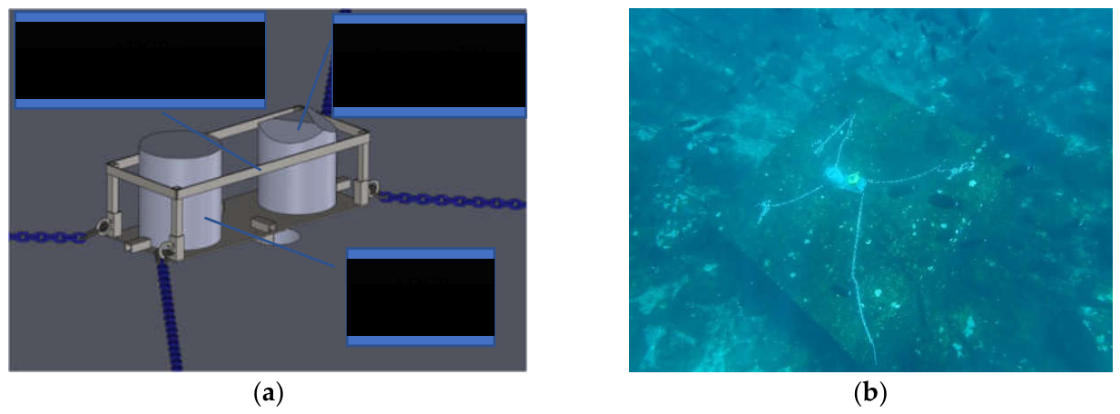
The survey was performed over a time interval of about 3 days. The instrument working principle is based on the acoustic doppler effect: three sonic beams are generated at the top of the ADCP device, the acoustic back-scattering from particles suspended in water is used to measure three velocity components, based on the Doppler generated frequency shift [13].
The time history of the velocity magnitude and direction is shown in Figure 4. The acquisition sample frequency is 10 seconds so that an average value over 10 second period is taken and saved. It must be noted that the Argonaut XR ADCP can measure the current speed at several distance, toward the sea surface, from its mounting position, averaging the speed over a set of measuring volumes (defined as “cells”) of assigned heights. In this application, ten cells were considered, each one having a height of 0.6 m. Specifically, the following configuration settings were considered (Table 1):
Moreover, the instrument is also capable to measure an overall speed, estimated over the entire water column (here indicated as “Single Overall Cell”), accounting for the possible variations of the water column height due to the tidal excursion.
2.2.2. Current Speed Measurements Results
All the measured velocity signals are reported in Figure 4, allowing a direct comparison of the time variation and of the effect of depth.
It has to be noted that, quite unexpectedly, the magnitude of the current speed in the observed portion of the water column seems to be relatively uniform with respect to depth. This could be partially attributed to the fact that the instrument was positioned on an existing concrete block at 1 m from the seabed, beside the fact that the first measurement cell is set at 0.5 m above the instrument itself.
It is worth to note that the last two cells close to the surface were discarded, since, due to the tidal excursion, such cells may be located above the effective water column extent or, nonetheless, they can be affected by the proximity to the water surface which could reduce the quality of the observed data.
The velocity data are expressed by the velocity magnitude with positive sign for eastward oriented flow.
The directionality of the current speed is illustrated using a water current direction rose, shown in Figure 5, highlighting the typical reversing pattern of tidal currents.
2.2.3. Tidal Height Measurements
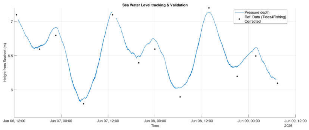
The Sontek YSI ADCP is also provided with a pressure sensor, allowing for the determination of the actual tidal surface elevation. The pressure-based tidal elevation measurements are compared to a set of reference data retrieved from a publicly available source [12]).
A good agreement between measured and publicly available data (Ref. Data in the legend) can generally be observed, with average percent difference of about 1.8% (ranging from -0.9% to 5%). It should also be remarked that the publicly available data, originally referred to the mean lower low water tide () level, have been corrected, shifting the tide reference level in order to match the pressure-based measurements, referred to the measurement site depth.
Figure 6.
Pressure sensor estimated depth compared to publicly available tidal height reference data. Note that the reference data have been corrected, in order to match the depth of the measurement site.
Figure 6.
Pressure sensor estimated depth compared to publicly available tidal height reference data. Note that the reference data have been corrected, in order to match the depth of the measurement site.
2.2.4. Bathymetric Survey
Moreover, a bathymetric survey was conducted, reconstructing the seabed depth distribution using a sonar measurement system in the area of interest (indicated in Figure 1b). In Figure 7a, the results of the bathymetric survey are shown in terms of isobathymetric curves; in Figure 7b a cross section showing a relatively constant seabed is shown, with minimum depth slightly above 8 m.
Considering the reported cross section, a relatively constant section depth can be observed. For conservativeness and simplicity, an idealized cross section shape was considered, assuming a flat central section with constant depth. The depth of the central part of the idealized channel shape is assumed conservatively equal to 7 m and a flat section width of approximately 300 m has been considered. The assumed simplified section is shown in Figure 8. The estimates of the annual energy resource are associated to the idealized section indicated in the figure.
2.3. Assumed Cross-Section Distribution of Tidal Current Speed
In order to estimate the energy transported through the considered section, a vertical speed profile has to be assumed. As will be subsequently discussed in more detail, in the site of interest at least part of the water column shows a relatively constant current speed; thus, in this study, the assumed vertical profile comprises two segments:
- constant speed segment: corresponding to the approximately uniform measure vertical distribution;
- 1/7th power law segment: below a given distance from the seabed the 1/7th power law is used to model the boundary layer close to the sea floor (as discussed later in sec. 3.2 and shown in Figure 15).
Such assumption on the vertical profile is subsequently used to determine the cross-section speed distribution used in eq. 1, where the current speed, , is considered as a function of time, , and vertical coordinate, , according to the following expression
where is the tidal current speed in the constant stream region and is the site depth.
The prediction of over a 1-year time interval is based on a correlation model developed in this study, as described in the next subsections.
2.4. Prediction Model for the Tidal Surface Elevation and Current Speed
2.4.1. Prediction of Tidal Height Variation with Experimental Corrections
As mentioned earlier, the measured data, combined with data from other sources and with tidal numerical estimation model, was used to predict the annual theoretical energy resource available in the considered site. This estimation, in combination with the considered bathymetry of the site, allowed us to perform an estimation of the real expected energy yield of a hypothetical farm made by a series of turbines rows arranged in an optimized layout. The basic model used to generate tidal current predictions relies on the FES2022 ocean tide model. For a given couple of geographic coordinates, several tidal components are available to be used in reconstructing the tidal height time history with a given timestep using the harmonic analysis technique. In particular, in this study a 10 min time interval has been used. In order to increase the accuracy of the model, the tidal height time history directly generated by the FES2022 model was corrected using a linear scaling approach was used. The direct FES2022 output time series was, in fact, calibrated to match the measured speed data. Since the measured tidal excursion showed a good agreement with the reference data retrieved from [12], as shown in Figure 6, the time history of tide level was adjusted to match the known reference data in the time interval of the measurement campaign, where such data are validated by comparison to the measured data, according to the following expression
where indicates the adjusted time series, represent the direct FES2022 model, is a scaling parameter, is an offset which also allow to account for possible differences in the reference tide level between the reference data and the model tide level reference, and is a time lag accounting for the possible difference in the time reference between the model and the reference data. The calibration coefficients are estimated using the least square method, the main results are shown in Figure 9 and Table 2.
The presence of a time lag is justified by the difference in time reference between the FES2022 model (which is based on the UTC standard time) and the reference data (which are reported in reference to the local time of the site).
After the adjustment, a full year time series of the tidal surface elevation can be generated, as shown for the year 2026 in Figure 10.
2.4.2. Prediction of Tidal Current Speed Variation with Experimental Corrections
Once the tidal height is known for a given time interval, in this study a prediction model is presented to estimate the annual time series of the tidal current speed in the site of interest. The presented model assumes a proportional relation between the tidal height slope and the current speed. The processed input data and correlation procedure between current speed and tidal height slope is summarized in Figure 11.
In particular, Figure 11a displays the current speed data recorded during the measurement campaign. To prepare the data for the correlation analysis, the raw ADCP measurements (blue line) were filtered (orange line) to dampen high-frequency oscillations. The velocity dataset utilizes the single overall variable cell measurement, representing a depth-averaged value. This approach is justified by the nearly uniform vertical velocity profile observed across the water column, as previously illustrated in Figure 4.
Concurrently, Figure 11b presents the raw measured tidal height (blue line) alongside a smoothed time series (orange line). The smoothing was performed using a moving average filter with a 360-sample window, selected looking for a balance between attenuating raw measurement oscillations and preserving the underlying physical trend. Subsequently, the tidal height slope was computed via a first-order numerical derivative of the smoothed tidal elevation time series. Finally, a least-squares linear regression was applied to correlate this calculated tidal slope with the filtered tidal current speed, as depicted in Figure 11c (red solid line and green dots, respectively).
Using the assumed approach, the tidal current speed time series over a given observation interval can be estimated, as shown in Figure 12.
The proposed tidal current prediction model enables the evaluation of the theoretical hydrokinetic resource and the expected energy yield of a specific tidal turbine deployed at the site, according to the approach described in sec. 2.1.
2.5. Analysis Code Implementation
In order to analyze the data and define the prediction model, a set of calculation scripts have been generated using the Python and MATLAB™ languages, partly generated with the support of the AI, mainly for data analysis and visualization purposes. The need to use two different languages is related to the availability of a library to access the results of the FES2022 model, while the main energy production calculations were conducted using MATLAB code dedicated to time series analysis, correlation and visualization.
3. Results and Discussion
Some of the results related to the experimental campaign were already discussed in the previous section, due to their strict relation with the approach used in the definition of the tidal current prediction model. In this section, after a brief revision and validation of the tidal current model, some results related to the site resource estimation are presented.
3.1. Prediction Model Validation
The main assumption of the proposed predictive model relies on a direct relationship between the tidal height slope and the magnitude of the tidal current. The validity of this assumption is evaluated through the coefficient of determination () derived from the linear regression shown in Figure 11c. The analysis yields an value of about 0.89, indicating a relatively high degree of correlation. While the data scatter in Figure 11c reveals that not all high-frequency variations in current speed are perfectly captured by this simplified linear relationship—likely due to localized turbulence or secondary hydrodynamic effects—at least the overall driving trend seems to be well represented.
Ultimately, the consistency of the proposed extrapolation approach is confirmed by comparing the model’s long-term velocity predictions against the independent, raw in-situ measurements, at least according to the short-term campaign data. As demonstrated in Figure 13, a good agreement is achieved between the reconstructed signal (red line in Figure 13) and the empirical data (black line in Figure 13), confirming that the synthesized tidal current profile provides a consistent baseline for the subsequent energy yield assessment.
3.2. Resource Estimation Results
Once the prediction model has been defined, all the information needed to perform a resource assessment is available, allowing the evaluation of the yearly time history of the power density, as shown in Figure 14 which summarizes the all the main physical quantities involved in the resource estimation process.
A maximum current speed of about 3.87 m/s is predicted by the model. Figure 14 also shows the predicted power density. The reported power density value is averaged over the water column. In fact, a vertical profile has been assumed for the current speed in the section, based on the measured data. The current speed in the observed part of the water column shows a relatively constant trend with depth, as previously shown in Figure 4. Thus, the ADCP measurement of the single overall variable cell has been considered representative of the whole current speed profile for the part of the water column above the measurement device, approximately from 1 m above the seabed up to the sea level. Below 1 m from the seabed a standard 1/7th power law has been considered to account for the near bottom boundary layer. A typical vertical profile assumed in this analysis is illustrated in Figure 15a. As explained in sec. 2.2.4, the assumed current speed distribution was integrated over the flat part of the idealized bathymetry (Figure 8), in this way the kinetic energy per unit time flowing through the considered cross section was calculated, as reported in Figure 15b. The integral over time of the energy per unit time passing through the considered cross section is assumed in this study as a measure of the overall resource in the area of interest, yielding an estimation of the expected theoretical resource of about .
It must be noted that the power density (indicated in the lower plot in Figure 14 as depth averaged power) as well as the total power and energy over the cross section reported in Figure 15 are estimated considering the presence of the boundary layer (as described in sec. 2.3).
A number of assumptions and simplifications was applied to derive the reported result on the theoretical resource for the site under consideration. A first assumption is related to the idealization of the cross section considered to estimate the amount of theoretically available energy: a constant depth section was considered in this study assuming a depth of 7 m, which was deemed representative of the effectively exploitable area for the possible installation of hydrokinetic turbines, based on the measured bathymetry. However, the definition of the effective layout of a future farm will require a detailed analysis of the optimal positioning of the installed turbine units.
Another simplification affecting the result is related to the assumption of the current speed distribution over the considered cross section. An almost uniform distribution was considered, accounting for a correction in the vertical profile due to the boundary layer, but assuming that the velocity profile is constant along the transverse direction. This is a strong assumption, mainly related to the availability of data only in a single measurement point. However, due to the preliminary character of this analysis this assumption was accepted to provide an initial estimate of the theoretical resource.
Furthermore, the proposed model assumes a linear relation between tidal current speed and tide height slope, trying to avoid the use of complex and computationally expensive 3D numerical fluid dynamic models in a preliminary assessment stage. Other attempts have been presented in literature to provide a quick preliminary estimation of the resource based on a basic knowledge of the tidal behavior in a given site. For example, in [14] a linear relation was established between a nondimensional parameter known as tidal coefficient, representing tide height, and the current speed. The simplified approach assumed in the present work aims at the same objective of reducing the computational cost of the resource prediction in early project stages. A relatively good correlation was observed between experimental and predicted current speed data, as was shown in Figure 11 and Figure 13, however, in more advanced development stages of a possible hydrokinetic turbine farm project more detailed numerical and experimental investigations will be required.
Another observation about the presented result is related to the theoretical meaning of the provided resource estimation. The estimated available energy has to be considered as an environmental characterization of the site under investigation. An approach to provide an estimation of the technical resource, which is the fraction of the theoretical resource effectively available for exploitation by a tidal energy plant [1], was considered in this study. A specific hydrokinetic turbine design, associated to a given power curve, has been assumed with the characteristics indicated in Table 3.
As a remainder, the power coefficient, , reported in the table above is defined as , where is the turbine power, is the water density, is the flow speed, is a reference surface assumed equal to the rotor disk area (). The power coefficient considered in this study takes into account the overall power conversion process, from the kinetic power of the flow to the electrical power delivered to the grid, accounting for hydrodynamic, mechanical and electrical efficiencies. In this work a value of 0.45 has been considered a plausible estimate for a typical hydrokinetic turbine in an initial plant design stage. The power coefficient is, in general, a function of the operating conditions of the turbine. In this study, the power coefficient is considered constant up to the condition at which the rated power is reached (maximum power for continuous operation of the generator); in this first part of the power curve a typical cubic dependency of the power output on the current speed is assumed. The rated current speed is the defined as the current speed at which the rated turbine power is reached. The cut-in and cut-out current speeds defines the current speed interval within which the turbine is operative.
Based on the above-mentioned assumptions, the power curve reported in Figure 16 was used to estimate the energy production of a single turbine.
For the considered case study, an expected annual energy production of about was predicted for a single turbine deployed at the installation site. The capacity factor, , is defined as the ratio between the effective energy production and the energy generated as if the turbine would continuously work at its rated power for a whole year (8760 h), according to the following expression
In the considered case, a value of the capacity factor of about was estimated. An analogous commonly used performance parameter is represented by the equivalent hours, , which is defined as the number of hours during which the plant should ideally work at its rated power to produce the effectively generated AEP, evaluated according to the following expression
In the considered case, a value of was approximately estimated.
The range of variation of the estimated capacity factor is relatively wide depending on the site of installation and on the characteristics of the specific tidal turbine. According to the results reported in some literature reference, such as [15,16], values of the capacity factor ranging between about 20% and 40% are reported. The results obtained in the present study are substantially in agreement with the indicated interval. However, further investigations, beyond the purpose of this work, which is mainly focused on a preliminary resource assessment, would be required to establish the economic viability of a possible plant.
To provide an estimate of the technical resource, a simplified layout of a possible plant comprising multiple turbine units was assumed. A single row of turbines with a fixed lateral spacing was considered, assuming a lateral distance, , between two adjacent turbine axes equal to 3 diameters, . Assuming a width of the exploitable area equal to , the number, , of installable turbines in a row can be estimated as . Based on this result, the annual energy production, , for a possible turbines plant is equal to
Comparing the energy production of a possible plant to the theoretical resource estimated earlier, we can finally determine a rough estimate of the fraction of theoretical resource practically exploitable for energy generation in the considered site and for the assumed technical characteristics of the plant:
It has to be noted that in this preliminary study the possible effect of the deployment of a farm with multiple turbine units on the tidal current resource has not yet been considered. The installed turbines can, in principle, act as sources of resistance to the tidal stream, particularly in the confined flow of a channel as in the considered case study, thereby possibly altering the effectively available resource. Further dedicated studies are needed to investigate this possibly significant topic, however, for the considered plant layout, only a relatively small fraction of the theoretical resource is effectively exploited, suggesting that the overall environmental effect of the assumed plant can be neglected at least in a preliminary stage of the analysis. In any case, since the bathymetry changes in entering Lac Ghoubet, probably more than one row of turbine can be deployed, and the rotor diameter can be much higher since the depth increases inside the Lac Ghoubet. These analyses are part of a future investigation needed to assess how the stream speed varies entering Lac Ghoubet.
5. Conclusions
A preliminary resource estimation was presented for the Grand Passage channel in the Ghoubbet-el-Kharab site. A short-term experimental campaign was conducted to gather the fundamental information about the bathymetry and the tidal current time history at the considered location. A prediction model for tidal current estimation was presented in this work, assuming a correlation between the tidal current speed and the slope of the tidal height (derivative of tidal height variation). A good agreement with experimental data was found for the observation interval of the test campaign. The prediction model was used to provide an estimation of the theoretical and technical resources available at the site of interest. Further investigations will be needed to assess the possibility to exploit larger areas than passage only investigating how the stream speed decays entering in Lac Ghoubet. Furthermore it is also necessary to investigate the possible effects of a given plant configuration on the environmental resource and the effective economic viability of a tidal stream project in the considered site.
Author Contributions
Conceptualization, D. Coiro.; methodology, D. Coiro; software, G. Troise; investigation, D. Coiro.; writing—original draft preparation, G. Troise.; writing—review and editing, D.Coiro, G. Troise.; visualization, G. Troise.; supervision, D. Coiro. All authors have read and agreed to the published version of the manuscript.
Funding
This research received no external funding.
Data Availability Statement
The original contributions presented in this study are included in the article. Further inquiries can be directed to the corresponding author.
Acknowledgments
The authors wish to thank Djibouti prime minister Abdoulkader Kamil Mohamed not only for his support in performing the analysis shown in the paper but also for his strong will to promote not only tidal stream clean energy but also other sources of renewable energy to make Djibouti a carbon free country. During the preparation of this study, the authors used Gemini, version 5.1. for the purposes of supporting data processing and visualization. The authors have reviewed and edited the output and take full responsibility for the content of this publication.
Conflicts of Interest
The authors declare no conflicts of interest.
Abbreviations
The following abbreviations are used in this manuscript:
| ADCP | Acoustic Doppler Current Profiler |
| AEP | Annual Energy Production |
| TEC | Tidal Energy Conversion (system) |
| SSH | Sea Surface Height |
| MLLW | Mean Lower Low Water |
| RMSE | Root Mean Square Error |
| MAE | Mean Absolute Error |
| CF | Capacity Factor |
References
- Coles, D. S.; Adcock, T. A. A.; Cornett, A.; Haas, K.; Jo, C. H.; Liu, H.; Miles, J.; Novo, P. G.; Thiébot, J. A review of global tidal stream energy resources. Proc.R.Soc. 2024, A481, 20240841. [Google Scholar] [CrossRef]
- Rivera, W. L.; Santos, V. S.; Morejón, M. B.; Quispe, E. C. Methodological Framework for Tidal Energy Assessment in Low-Energy Tropical Estuaries: An ADCP-Calibrated Hydrodynamic and Techno-Economic Approach. Water 2026, 18, 1370. [Google Scholar] [CrossRef]
- Lifschitz, J.; Coiro, D.; Troise, G.; Giaquinta, H.; Lazcano, F.; Cristofaro, N. d. Kinetic energy of tidal currents in the province of Chubut, Argentina. Int. Mar. Energy J. 2022, vol. 5(n. 1). [Google Scholar] [CrossRef]
- Legrand, C. Assessment of Tidal Energy Resource; EMEC: London, UK, 2009. [Google Scholar]
- The University of Edinburgh. Preliminary Tidal Current Energy Device Performance Protocol; DTI, 2007. [Google Scholar]
- GEBCO Compilation Group. GEBCO Bathymetric Compilation Group 2026(2026). The GEBCO_2026 Grid—a continuous terrain model for oceans and land at 15 arc-second intervals; NERC EDS British Oceanographic Data Centre NOC, 2026. [Google Scholar] [CrossRef]
- Djibouti Ministry of Equipement and Transport Maritime Affairs (in cooperation with Japan International cooperation Agency). «The preparatory survey on the project for reinforcement of maritime transport capacity between Djibouti and Tadjoura,». 2019, 2019.
- Omar, Y. M.; Memery, L.; Carton e, X.; Daher, A. Effects of Monsoon Winds and Topographical Features on the Vertical Thermohaline and Biogeochemical Structure in the Gulf of Tadjourah (Djibouti). Open J. Mar. Sci. 2016, n. 6, 440–455. [Google Scholar] [CrossRef]
- Madah, F.; Mayerle, R.; Bruss e, G.; Bento, J. Characteristics of Tides in the Red Sea Region, a Numerical Model Study. Open J. Mar. Sci. 2016, n. 5, 193–209. [Google Scholar]
- AVISO+. FES2022 (Finite Element Solution) Ocean Tide product handbook; AVISO+, 2026. [Google Scholar]
- Lyard, F. H.; Allain, D. J.; Cancet, M.; Carrère, L.; Picot, N. FES2014 global ocean tides atlas: design and performances. Ocean Sci. 2020, vol. 17, 615–649. [Google Scholar] [CrossRef]
- tides4fishing, «Tides4Fishing/https://tides4fishing.com/dj/djibouti/djibouti,» tides4fishing. Available online: https://tides4fishing.com/.
- Argonaut SL/SW/XR Technical Manual; Sontek YSI, 2004.
- Tawil, T. E.; Guillou, N.; Charpentie e, J.-F.; Benbouzid, M. On Tidal Current Velocity Vector Time Series Prediction: A Comparative Study for a French High Tidal Energy Potential Site. J. Mar. Sci. Eng. MDPI 2019, vol. 7(n. 46). [Google Scholar]
- IRENA. Tidal Energy—Technology brief; IRENA, 2014. [Google Scholar]
- Goss, Z. L.; Coles, D. S.; Piggott, M. D. Identifying economically viable tidal sites within the Alderney Race through optimization of levelized cost of energy. Phylosofical Trans. R. Soc. 2020, A 378. [Google Scholar] [CrossRef] [PubMed]
Figure 1.
General view of the site location. (a) Overall area of interest; (b) detail of the Grand Passe area (approximate ingoing and outgoing stream directions).
Figure 1.
General view of the site location. (a) Overall area of interest; (b) detail of the Grand Passe area (approximate ingoing and outgoing stream directions).
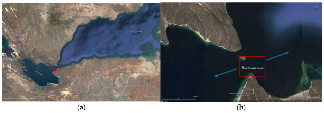
Figure 2.
Bathymetry of the area of interest based on literature data [6].
Figure 2.
Bathymetry of the area of interest based on literature data [6].
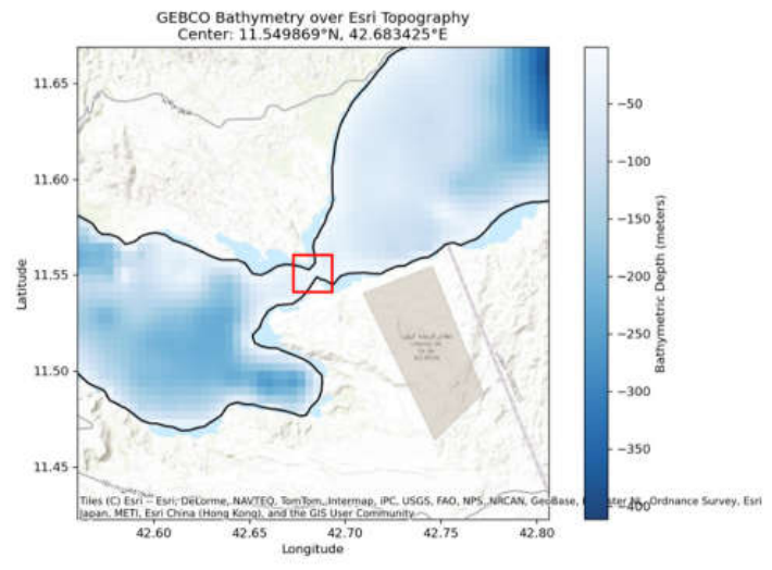
Figure 4.
Time histories of the measured current velocity magnitude for all the measurement cells. Note that the sign of the current velocity is based on the direction of tidal flow, assuming a positive sign for eastward current directions. The upper plot shows the signed water current speed (with sign defined according to the East/West direction; positive values indicate eastbound current), while the lower plot shows the time history of current direction with respect to north. The color scale indicates the depth.
Figure 4.
Time histories of the measured current velocity magnitude for all the measurement cells. Note that the sign of the current velocity is based on the direction of tidal flow, assuming a positive sign for eastward current directions. The upper plot shows the signed water current speed (with sign defined according to the East/West direction; positive values indicate eastbound current), while the lower plot shows the time history of current direction with respect to north. The color scale indicates the depth.
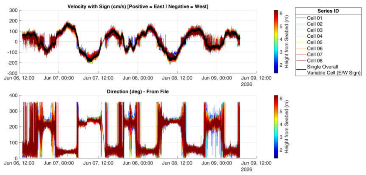
Figure 5.
Water current direction rose.
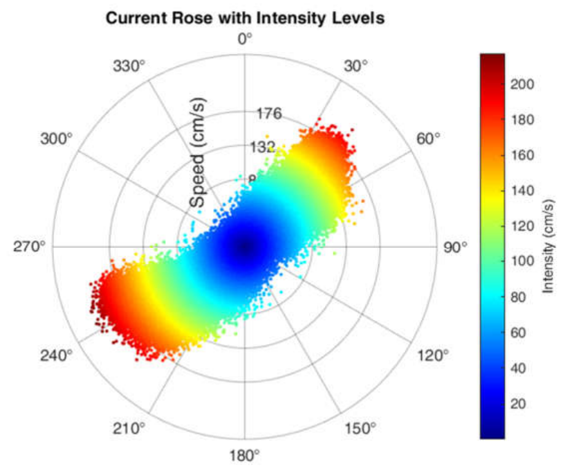
Figure 7.
Measured bathymetry in the area of interest. (a) Isobathymetric curves (black solid lines), measurement points (black dotted scatter) and section transect for representative cross section (red continuous line). (b) Section bathymetric profile along the indicated transect.
Figure 7.
Measured bathymetry in the area of interest. (a) Isobathymetric curves (black solid lines), measurement points (black dotted scatter) and section transect for representative cross section (red continuous line). (b) Section bathymetric profile along the indicated transect.
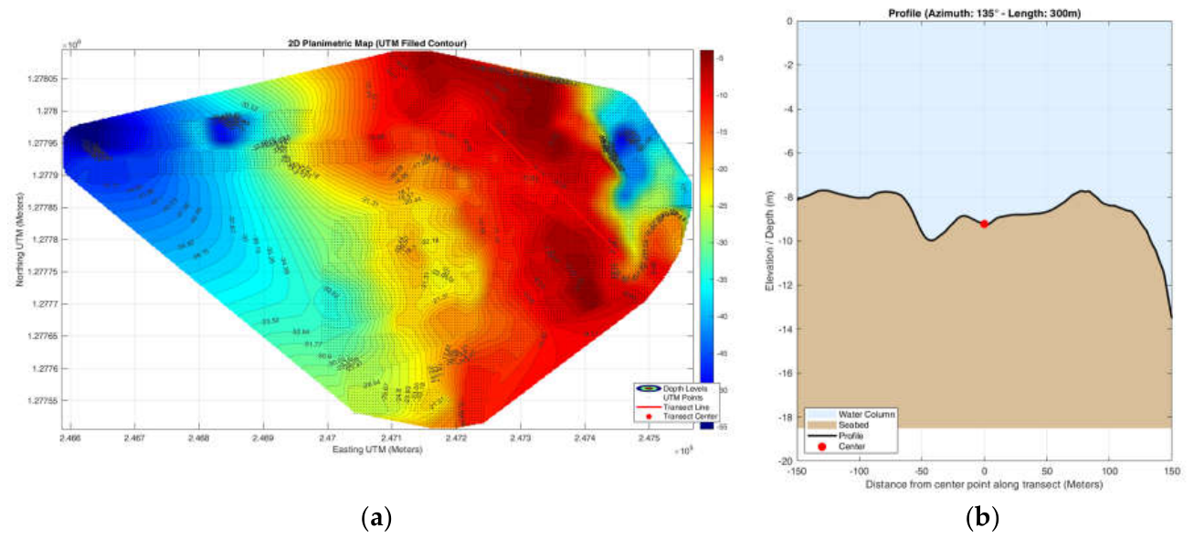
Figure 8.
Idealized channel section. (The dashed red line represents the area considered for the preliminary estimation of annual energy resource; the blue line represents the assumed mean water level).
Figure 8.
Idealized channel section. (The dashed red line represents the area considered for the preliminary estimation of annual energy resource; the blue line represents the assumed mean water level).
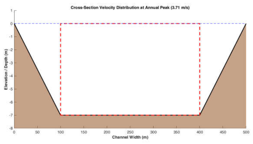
Figure 9.
Calibration of the FES2022 model results to validated reference data. Red dots represent reference data, green solid line represents original FES2022 model output, magenta solid line represents the calibrated time history.
Figure 9.
Calibration of the FES2022 model results to validated reference data. Red dots represent reference data, green solid line represents original FES2022 model output, magenta solid line represents the calibrated time history.
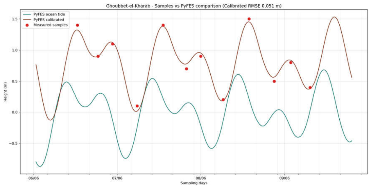
Figure 10.
Annual predicted tidal height time series, based on the FES2022 model for the year 2026.
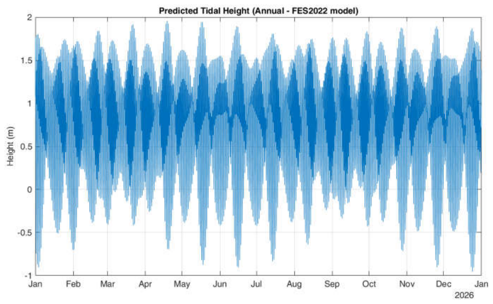
Figure 11.
Tidal current speed prediction model. (a) Tidal current velocity measurements (raw data in blue, filtered data in orange); (b) tidal height in the measurement interval; (c) correlation between current speed and tidal height slope (green dots) and linear regression (red solid line).
Figure 11.
Tidal current speed prediction model. (a) Tidal current velocity measurements (raw data in blue, filtered data in orange); (b) tidal height in the measurement interval; (c) correlation between current speed and tidal height slope (green dots) and linear regression (red solid line).
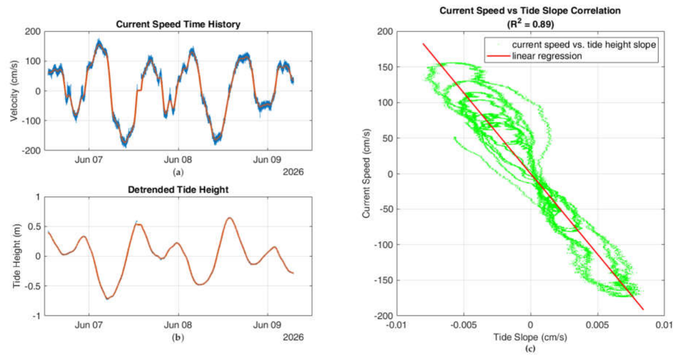
Figure 12.
Tidal current speed model prediction over a 1-year long time interval.
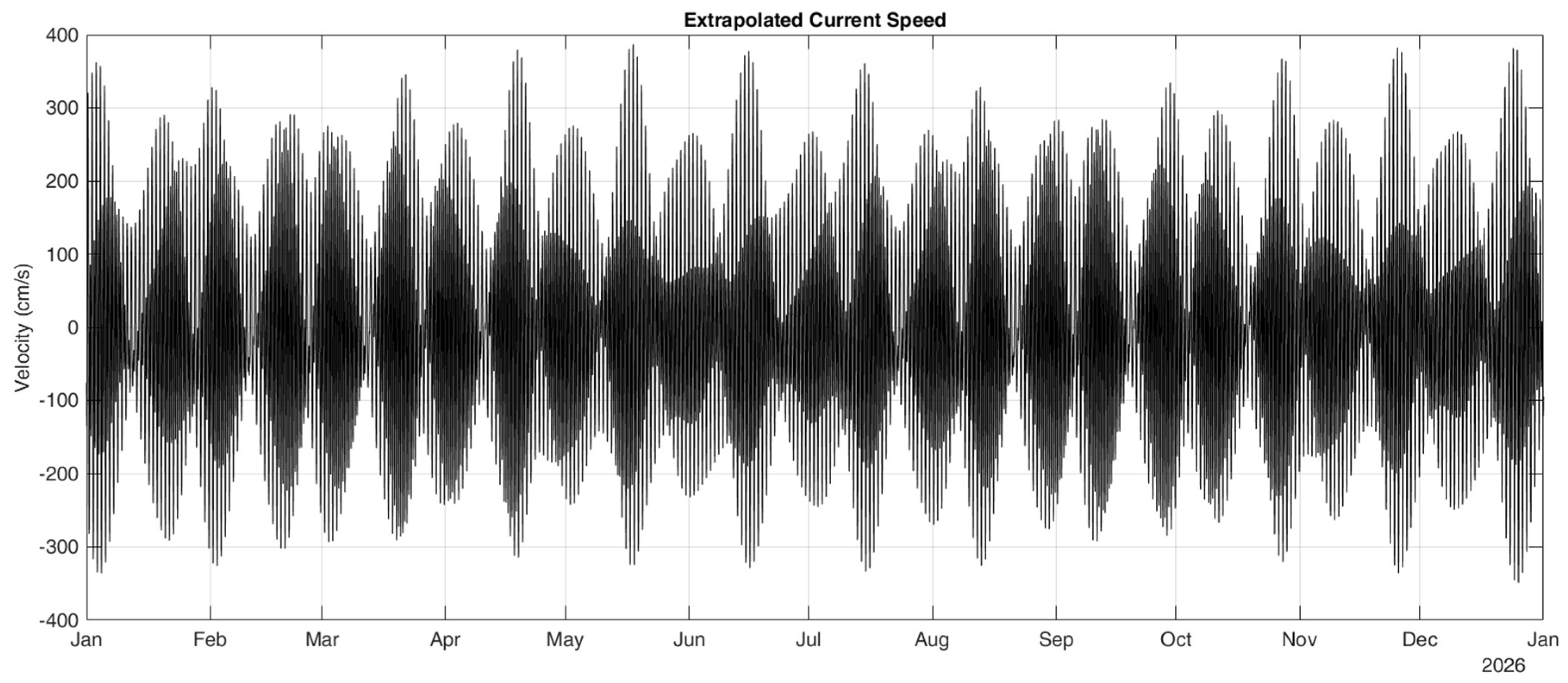
Figure 13.
Tidal current speed variation over an observation interval of about half a month, comprising the duration of the test campaign (from June 6 to 9, 2026). Raw measured speed data (black solid line) compared to the results of the prediction model (red solid line).
Figure 13.
Tidal current speed variation over an observation interval of about half a month, comprising the duration of the test campaign (from June 6 to 9, 2026). Raw measured speed data (black solid line) compared to the results of the prediction model (red solid line).
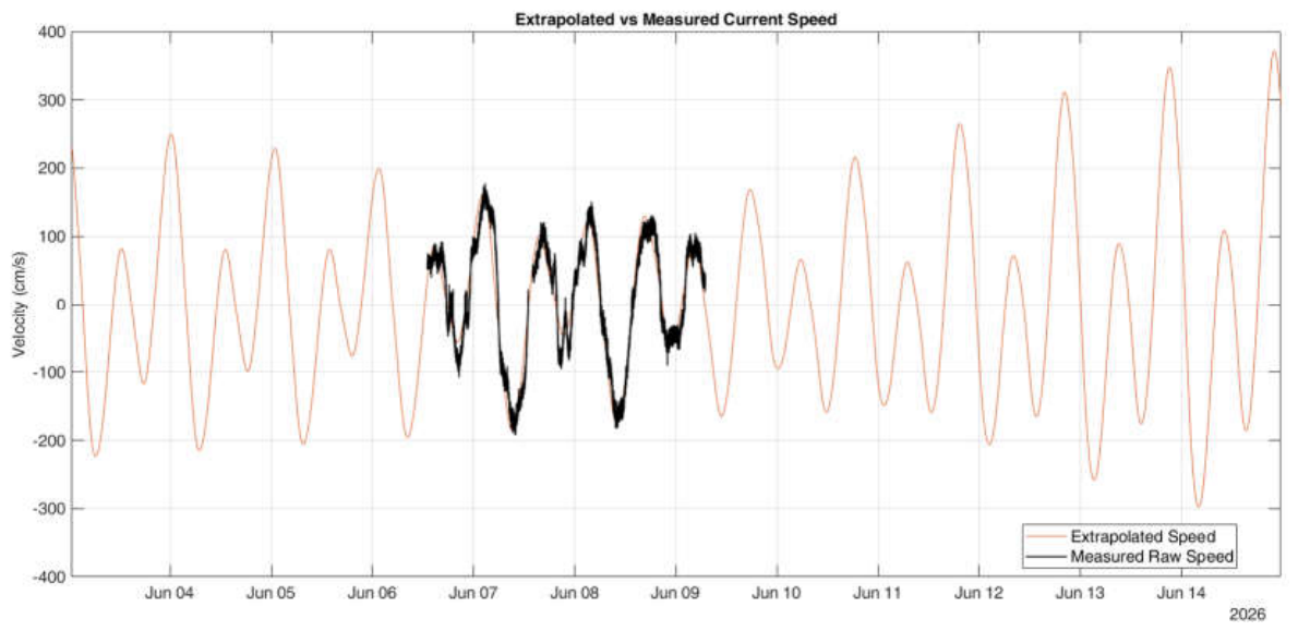
Figure 14.
Assumed tidal model for a 1-year long time period. Upper plot shows the predicted annual tidal height; the middle graph reports the extrapolated current speed based on the assumed methodology; the lower graph shows the predicted power density (power per unit area) for the considered site, according to the predicted current speed.
Figure 14.
Assumed tidal model for a 1-year long time period. Upper plot shows the predicted annual tidal height; the middle graph reports the extrapolated current speed based on the assumed methodology; the lower graph shows the predicted power density (power per unit area) for the considered site, according to the predicted current speed.
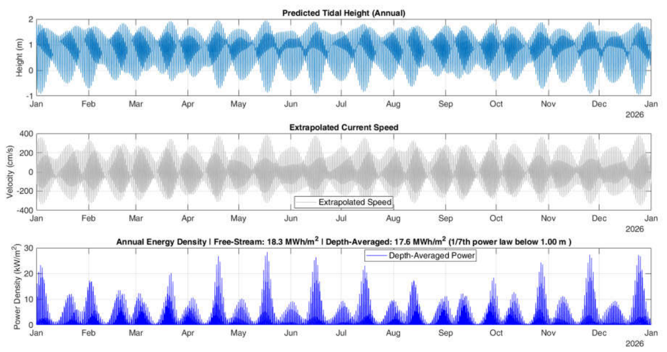
Figure 15.
(a)Assumed vertical profile; (b) overall energy per unit time (power) integrated on the central flat part of the idealized bathymetry in Figure 8.
Figure 15.
(a)Assumed vertical profile; (b) overall energy per unit time (power) integrated on the central flat part of the idealized bathymetry in Figure 8.
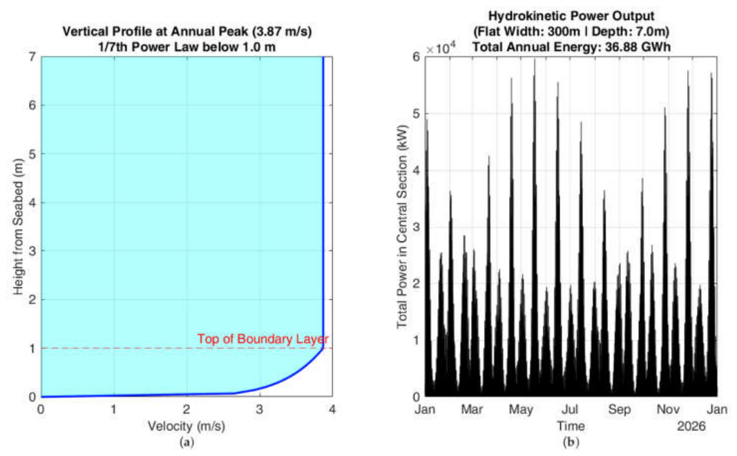
Figure 16.
(a) Assumed turbine power curve. (b) Cross section velocity distribution and turbine size for estimation of single turbine energy production.
Figure 16.
(a) Assumed turbine power curve. (b) Cross section velocity distribution and turbine size for estimation of single turbine energy production.
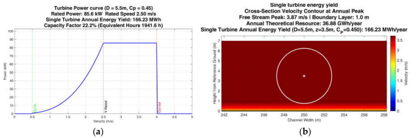

Table 1.
ADCP main mounting and configuration parameters.
| ADCP Parameter | Value | Note |
|---|---|---|
| ADCP mounting height | 1.18 m | Distance of the sensor top from seabed (m) |
| Blank distance | 0.5 m | Distance between sensor top and first measuring cell (m) |
| Cell size | 0.6 m | Vertical size of each cell (m) |
Table 2.
Tidal height model calibration parameters.
| Calibrated Model Parameter |
Value | Units | Note |
|---|---|---|---|
| +0.801 | m | Offset | |
| 1.068 | Scale | ||
| -3.00 | hours | Lag | |
| RMSE | 0.051 | m | Root mean square error of calibrated data |
| MAE | 0.043 | m | Mean absolute error of calibrated data |
Table 3.
Characteristics of the hydrokinetic turbine design assumed for the preliminary estimation of the technical resource.
Table 3.
Characteristics of the hydrokinetic turbine design assumed for the preliminary estimation of the technical resource.
| Parameter | Value | Units | Note |
|---|---|---|---|
| 5.5 | m | Rotor Diameter | |
| 3.5 | m | Hub height above seabed | |
| 0.45 | Overall power coefficient | ||
| 0.3 | m/s | Cut-in current speed | |
| 4 | m/s | Cut-out current speed | |
| 2.5 | m/s | Rated current speed | |
| 85 | kW | Generator rated power |
Disclaimer/Publisher’s Note: The statements, opinions and data contained in all publications are solely those of the individual author(s) and contributor(s) and not of MDPI and/or the editor(s). MDPI and/or the editor(s) disclaim responsibility for any injury to people or property resulting from any ideas, methods, instructions or products referred to in the content. |
© 2026 by the authors. Licensee MDPI, Basel, Switzerland. This article is an open access article distributed under the terms and conditions of the Creative Commons Attribution (CC BY) license (http://creativecommons.org/licenses/by/4.0/).
Copyright: This open access article is published under a Creative Commons CC BY 4.0 license, which permit the free download, distribution, and reuse, provided that the author and preprint are cited in any reuse.