Deep Learning-Based Radiotherapy Automatic Segmentation Workflow (DRAW): Initial Experience with a Distributed Open-Source Client-Server-Based Autosegmentation System Deployed in a Low- and Middle-Income Nation

Sougata Maity; Santam Chakraborty; Sandip Dutta; Koustav Ghosh; Indranil Mallick; Sanjoy Chatterjee; Rimpa Basu Achari; Tapesh Bhattacharyya; Arunsingh Moses; Divyani Chowdhury; Sayan Chakraborty; Sandip Sarkar; Kanishka Sarkar; Paromita Adhikari; Pallabi Saha; Soumya Kanti Ghosh; Jayanta Mukhopadhyay

doi:10.20944/preprints202607.1916.v1

Submitted:

24 July 2026

Posted:

27 July 2026

You are already at the latest version

Abstract

Introduction: Automatic segmentation of target volumes and organs at risk may save time and reduce inter-observer variability. However, commercial systems are costly, difficult to customise, and often poorly represent local populations. We developed a deep learning-based automatic segmentation system (DRAW), based on a client-server architecture using a decoupled inference layer to enable on-demand use of computational resources. We report the initial deployment experience and performance across two centres.Materials and Methods: The DRAW system was deployed at two geographically distant centres. System uptime, successful segmentation rate, and segmentation time were recorded. Spatial overlap metrics, including the Dice similarity coefficient (DSC), Dice Jaccard coefficient (DJC), 95th percentile Hausdorff distance (HD95), surface Dice similarity coefficient (sDSC), and mean distance to conformity (MDC), were computed for a sampled subset where automatic segmentation and manually modified structures were available. A qualitative assessment of the extent of contour modification required was performed independently at one centre. Inter-centre differences were assessed using independent-samples t-tests.Results: Between April 2025 and April 2026, 4215 of 4303 uploaded series (98%) were successfully segmented. The API server uptime exceeded 99.5%. Median segmentation time was 20.2 minutes. Quantitative evaluation of segmented structures was performed in 380 patients. Aggregated mean DSC was 0.81 at Centre A and 0.78 at Centre B. Other spatial overlap metrics also showed a lower performance in Centre B. On qualitative review at Centre B, no modification was required for 24% of structures, while major and minor modifications were required for 33% and 31% of structures, respectively.Conclusion: The DRAW system was deployed and maintained across two centres with acceptable performance. Differences in model performance between the training and external centre indicate the need for more robust training. Open-source tools can reduce barriers to adopting automatic segmentation in resource-constrained settings.

Keywords:

radiotherapy

;

automatic segmentation

;

deep learning

;

low-middle income

Subject:

Biology and Life Sciences - Life Sciences

Introduction

Modern precision radiotherapy depends on accurate segmentation of target volumes and organs at risk. This process is time-consuming and subject to significant inter- and intra-observer variability [1]. Automatic segmentation saves valuable time and additionally reduces variability in contouring [2,3].

Automatic segmentation is not a new technology, and several commercial systems already support it [4]. However, the key challenges in adopting commercial automatic segmentation systems include high cost, vendor lock-in, a lack of representation of the local population in the training dataset, and limited capability to customise automatic segmentation models [3,5,6]. In low- and middle-income countries (LMIC) with limited resources and technical know-how, deploying these models is not trivial. Given these challenges, we set up a project to develop a deep learning-based radiotherapy automatic segmentation workflow (DRAW) in 2024 [7]. This system was first deployed at a tertiary cancer centre in an urban area of Eastern India. During this process, we focused on developing a simple pipeline to train new models on our own data and set up the inference pipeline. Initial results were quite promising, and from our initial attempt at developing a prostate cancer automatic segmentation model, we soon expanded to include other cancer sites like gynaecological cancers, head and neck cancer, brain tumours, and breast cancers [8].

However, this initial deployment still relied on the availability of a local workstation equipped with a Graphics Processing Unit (GPU). After informal discussions with colleagues at other oncology centres, we realised that most centres lacked the technical know-how and resources to deploy this pipeline in their local settings once they had purchased adequate computing hardware. Furthermore, contouring practices varied across centres, which meant they would want a customisable system and the ability to determine how they wanted a specific volume delineated. Finally, there was a perceived need to make the performance metrics available for an open review. In 2025, we redesigned the architecture to support these requirements.

To be cost-efficient and lower the barrier to entry, we opted for a client-server architecture, in which multiple thin clients upload Digital Imaging and Communications in Medicine (DICOM) data to a centralised cloud server for automatic segmentation. To maintain patient privacy, DICOM data was de-identified before export. Finally, we decoupled the inference layer from the server, enabling us to use expensive, energy-consuming GPU resources only on demand.

The DRAW system comprises three components: a client, an application programming interface (API) server, and an inference pipeline. The DRAW client can be deployed on any modern desktop operating system using Docker [9]. The prediction pipeline code can be deployed using ephemeral Docker containers on the cloud. The DRAW client supports asynchronous task processing using Celery and also serves as a DICOM server (using Pynetdicom) [10,11]. Once installed and configured, the system automatically processes incoming DICOM images, reads the metadata and matches an automatic segmentation template to the series. Subsequently, it de-identifies the images, removing identifying information in accordance with HIPAA safe harbour standards, and then exports them to the API server. The DRAW API server verifies the images and then transfers them to an orchestration layer [12]. The orchestration layer starts an ephemeral GPU machine that runs inference on the DICOM data, using information from the template to determine which models to use. Once segmentation is complete, the DRAW API server retrieves the RTStructureSet file, which the DRAW Client then downloads. The DRAW client then reidentifies the RTStructureSet file and sends it to the central storage. The DRAW API server also deletes the deidentified images and RTStructureSet file after a successful transfer. The full system design documentation is available in Supplementary Appendix I.

This manuscript outlines the key system features, initial deployment experience, system performance across two Centres and some challenges encountered during this period. The system performance across two Centres is of particular interest, as all models were trained exclusively on patients who underwent imaging at Centre A.

Methodology

The current study is a retrospective case series of the first set of consecutive patients segmented with the redesigned DRAW automatic segmentation system at two centres. The system was first deployed at our centre and then at another charitable cancer centre in a Tier II city in Eastern India.

Performance evaluation was conducted over 13 months, from 17th April 2025 to 17th May 2026, to allow sufficient assessment of the system's performance. Three key performance indicators were used to measure the system performance:

System uptime: Defined as the percentage of the total deployment period during which the DRAW system API was unavailable.
Successful segmentation rate: This was defined as the ratio of the total number of DICOM series where an automatically segmented structure set was generated to the total number of cases sent for segmentation
Segmentation time: This was measured as the time interval in minutes between the case being uploaded to the DRAW API server and its successful download by the DRAW client.

To assess autosegmentation accuracy, we computed several spatial overlap metrics between manually edited and autosegmented contours for a selected group of patients during the first five months after system installation. The computed metrics included the volumetric Dice similarity index (DSC) [13], Dice Jaccard Coefficient (DJC) [14], 95th percentile of the Hausdorff distance (HD.95) [15], surface DSC (sDSC), and mean distance to conformity (MDC) [16] (see Appendix II for the definitions). These metrics were computed for each automatically segmented structure in each selected patient using the COMET package [17]. For patient selection, the following rules were applied:

If a cancer site had more than 40 patients for a given centre, then consecutive sampling was used to select 40 patients.
If there were fewer than 40 cases, then all available cases were included

While spatial overlap metrics and distance measures can provide quantitative estimates of contour quality, a qualitative evaluation is also important. This is because in radiotherapy, small errors in target volume delineation can have a disproportionately high impact on the tumour control probability and normal tissue complication probabilities. As this was a qualitative and subjective assessment, we opted to perform it only in Centre B, where senior clinical oncologists perform all volume delineation and whose data were not used for model training. A paper case record form was provided, which requested that the oncologist rate the extent of modification required into three categories: major modification, minor modification, and no modification. As this was a subjective qualitative evaluation, no specific distance measures were recommended, and the experienced oncologists were asked to use their judgment in categorising the extent.

For quantitative metrics, descriptive summaries are provided for each metric as the mean and standard deviation. Centre-wise means were computed for all structures. In addition, structure-group-wise metrics have also been reported for the two centres. To determine differences in model performance between the two centres, an independent-samples t-test was performed. Given the difference in the numbers of cases between the two centres, equality of variance was assessed using Levene’s test [18]. This test yielded p-values < 0.05, resulting in the rejection of the null hypothesis of equal variance between centres. Hence, the test results are reported assuming unequal variances. Despite multiple testing, we opted to keep a nominal p-value of 0.05 as it was more conservative than evaluating statistical significance with a lower p-value after a Bonferroni correction [19]. As this was an audit of the performance of an existing service and de-identified data were used to compute spatial overlap metrics and qualitative feedback, institutional ethics approval was not required.

Results

The DRAW system was made operational on April 9th 2025, at Centre A and on 23rd April 2025 at Centre B. Since that time till April 30th 2026, a total of 4215 CT scan series have been successfully segmented, representing 98% of the total uploaded series. Centre A uploaded 3492 (83%) cases, and Centre B uploaded 723 (17%) cases. The noted failures occurred when the GPU machines were terminated prematurely by the cloud service provider due to resource constraints. In these instances, manually retriggering the automatic segmentation resulted in successful segmentation.

The median processing time was 20.2 minutes (interquartile range: 16.9-28.9 minutes). However, the distribution was right-skewed as shown in Figure 1. This was observed during two particular episodes. First, for a temporary period of 2 weeks in December 2025, when GPU resources were not available on demand during the daytime in the cloud service provider, segmentation was started only after 1800 hours. Second, in one instance, more than 249 cases were uploaded from Centre B in a single day for automatic segmentation due to a client misconfiguration, resulting in all old cases being segmented within 1 hour. If that single day was excluded, then the 80th, 85th and 90th percentiles of processing time were 24.5, 29.5, and 50.36 minutes, respectively.

The DRAW API Server has consistently demonstrated high uptime, with availability exceeding 99.5%. Downtimes were mostly linked to the unavailability of GPU-based virtual machines at the cloud service provider's end. Regarding the DRAW client, we encountered two downtime-related issues. In Centre A, the hard disk storage space was exhausted on a Friday, necessitating a three-day downtime for system cleaning and reinitialization. In Centre B, network issues unrelated to the client system prevented file transfers for 3 days. Aside from these issues, no further system downtime was observed during this period.

Data for quantitative evaluation was collected over the period from April 17th, 2025, to September 23rd, 2025. The total number of segmented patients at Centre A and B was 1113 and 191, respectively. The Centre A dataset included 1193 unique DICOM studies and 1326 unique series, whereas the Centre B dataset included 194 unique studies and 199 unique series. The distribution of cancer sites at Centre A was as follows: Breast (n = 474, 36%), Head and Neck (n = 332, 25%), Lung (n = 162, 12%), Brain (n = 136, 10%), Prostate (n = 85, 6.4%), Cervix (n = 77, 5.8%), Rectum (n=54, 4.1%), Others (n=6, 0.7% ). At Centre B, the distribution was Head and Neck (n = 96, 48%), Breast (n = 42, 21%), Cervix (n = 23, 12%), Lung (n = 23, 12%), Prostate (n = 4, 2%), Rectum (n=7, 4%), Bladder (n=2, 0.5%) and others (n = 2, 0.5%). Table 1 shows the demographics and cancer site for a subset of these cases for which quantitative analysis was performed, based on the selection criteria prespecified in the methodology. It should also be noted that the delineated structure types often overlapped across cancer sites. For example, several structures (e.g., brain, spinal cord) were delineated at different sites, so although there were no brain cases in Centre B, brain structures were segmented there as well.

Results of the quantitative analysis of the different spatial overlap metrics, aggregated across the Centres, are shown in Table 2. Figure 2 shows the summary visualisation for these aggregated metrics across centres for the different structure groups. As can be seen, there were statistically significant differences in model performance across the two centres: DSC, DJC, HD.95, Surface DSC, Under MDC, and Over MDC. Regions of interest where the Dice similarity coefficient and the mean distance to conformity were 1 and 0 were considered to be used without modification. Overall, 7838 of 5920 structures (76%; 95% confidence interval 75%, 76%) were modified. At Centre A, 1314 of 5571 structures (24%, 95% CI: 22% - 25%) were not modified. At Centre B, 604 of 2267 structures (27%; 95% CI 25% - 29%) were not modified (Chi-square p=0.004). Appendix II Table 2 has the comparative metrics for each structure reported for the two centres.

Qualitative feedback was received from two clinical oncologists for 34 unique patients at Centre B, with 551 structures autosegmented there. The distribution of cancer sites is as follows: Head & Neck (n = 20, 59%), Breast (n = 9, 26%), Lung (n = 2, 6%) and Rectum (n = 3, 9%). Notably, qualitative assessments were not available for all patients who underwent quantitative assessment. All but seven patients required a mix of major and minor modifications. These seven (6 Breast and 1 Head Neck) required only minor modifications across all structures. Overall, major modifications were required in 180 structures (33%), and minor modifications were required in 169 (31%). Aggregated analysis of the major/minor modification rates is presented in Table 3. The oncologists reported that the existing contours had to be completely redrawn for 86 (24.5%) of the structures (most commonly for the spinal cord, mandible, lens and optic chiasm). Major modifications due to incorrect side assignments were noted in 31 (9%) structures (most commonly for the cochlea, optic nerve, and lens). Table 3 (Appendix 4) presents a comparison of quantitative metrics for structures where major and minor modifications were required. All spatial overlap metrics were worse in patients with major modifications than in those with minor modifications.

Contour modification times were reported for 20 patients. Analysis of the modification time showed that the mean time to modify the contours was 20 minutes (standard deviation 10 minutes). The average number of major modifications in patients with contouring modification time of 20 minutes or less was 1 (SD: 1), versus 7 (SD: 3) in patients with modification time greater than 20 minutes.

Discussion

The present study demonstrates that an efficient, distributed, deep learning-based automatic segmentation system can be deployed in resource-constrained settings with limited user involvement after installation and configuration. We intentionally designed the system using open-source software not only to reduce development and licensing costs but also to accelerate development. Expensive, energy-intensive GPU resources are used on demand, as this suits radiotherapy workloads, where images for automatic segmentation are acquired over daytime working hours. By separating our system from reliance on commercial treatment planning systems, we have ensured that the output can be used irrespective of the vendors. For example, in Centre A, Varian and Accuray treatment planning are used, while in Centre B, Elekta’s treatment planning system is used. The training and inference pipeline was designed using the well-known nnUnet semantic segmentation framework [20]. The nnU-Net framework has consistently achieved high performance in multiple real-world environments and challenges.

The DRAW system has been designed to provide a complete pipeline for model training and inference. At this stage, the pipeline has been used to train 62 models covering 213 structures. The system not only covers automatic segmentation of anatomical organs and clinical target volumes (both nodal and primary) but has also been extended to segment planning structures for treatment planning. The available models have been sequentially improved by retraining them on a larger sample of cases. Currently, new models can be trained within one week if a curated dataset is available to accommodate new target volume delineation protocols and guidelines.

The model performance metrics, data source, and guidelines for delineating the structures are publicly available on the DRAW website (https://draw.chavi.ai). The DRAW client provides the functionality for a “model mart”, where the user can pick and choose the models and structures that they wish to be automatically segmented. As the number of models and structures increases, the DRAW system can flexibly accommodate multiple ways of delineating the same volume. The DRAW client and DRAW API server are decoupled from the inference layer, which means that, in the future, more advanced segmentation frameworks can also be used.

Nonetheless, several limitations need to be acknowledged. The DRAW system is not the first client-server-based automatic segmentation system and is unlikely to be the last. Two of the most well-known commercial systems in this area, MIRADA DLCXpert and MVISION Contour+, provide similar functionality [4,21,22]. The performance of the MIRADA and MVISION systems has been evaluated as part of a multi-vendor comparison by Doolan et al., who found that none of the evaluated systems was demonstrably superior to others, and that performance across sites was variable [4]. The aggregated mean DSCs for the MIRADA and MVISION systems were 0.82 and 0.88, respectively. However, in this study, a qualitative evaluation of the contours was not performed. A comparative summary of the DSC for the key structures is shown in Appendix II, Table 4, and values for the MIRADA and MVISION systems have been taken from Doolan et al [4]. Values for the DRAW system are those obtained during model validation.

An open source application, OSAIRIS, using a similar client-server architecture, has also been developed by Cambridge University and has been in clinical use for specific clinical sites [23]. The performance of this system was evaluated by Constantinou et al., who compared it against two commercial systems and found that spatial accuracy was comparable for Head Neck and superior for prostate cancer. The authors also evaluated the system's performance qualitatively by asking the oncologists whether the contours required major or minor modifications or were acceptable. For head and neck and prostate cancers, the no-modification rates were 67% and 59%, respectively [24]. It should, however, be noted that the qualitative evaluation was conducted at the centre where the tool was developed, whilst ours was conducted at a separate centre.

Other notable limitations include a retrospective design and a lack of a formal sample size calculation. Evaluation was performed at two centres, and qualitative assessments were available for a subset of patients. The decision to restrict the qualitative evaluation to Centre B was made to avoid bias, as the models were trained in Centre A. The performance drop in Centre B is to be expected, given that the total number of patients in the largest training dataset at the time was around 60. Nonetheless, the overall system performance was deemed acceptable, and Centre B has continued to use the system. When the system was initially developed, the contours were somewhat jagged, and small disconnected “blobs” were observed and sometimes segmented on the incorrect side. All of these issues have been addressed by implementing a custom post-processing chain that incorporates contour smoothing, removal of degenerate, disconnected segments, and removal of contours drawn on the incorrect side. Further prospective evaluation of model performance is also planned in other centres.

Conclusion

An in-house-developed, open-source, deep learning-based automatic segmentation system was successfully deployed. This study provides evidence that these open-source tools can be used to develop robust applications that not only save time but also lower barriers to entry in LMIC.

References

Guzene, L.; Beddok, A.; Nioche, C.; Modzelewski, R.; Loiseau, C.; Salleron, J.; et al. Assessing interobserver variability in the delineation of structures in radiation oncology: A systematic review. Int. J. Radiat. Oncol. Biol. Phys. 2023, 115, 1047–60. [Google Scholar] [CrossRef] [PubMed]
Radici, L.; Ferrario, S.; Borca, V.C.; Cante, D.; Paolini, M.; Piva, C.; et al. Implementation of a commercial deep learning-based auto segmentation software in radiotherapy: Evaluation of effectiveness and impact on workflow. Life 2022, 12, 2088. [Google Scholar] [CrossRef] [PubMed]
Hu, Y.; Nguyen, H.; Smith, C.; Chen, T.; Byrne, M.; Archibald-Heeren, B.; et al. Clinical assessment of a novel machine-learning automated contouring tool for radiotherapy planning. J. Appl. Clin. Med. Phys. 2023, 24, e13949. [Google Scholar] [CrossRef] [PubMed]
Doolan, P.J.; Charalambous, S.; Roussakis, Y.; Leczynski, A.; Peratikou, M.; Benjamin, M.; et al. A clinical evaluation of the performance of five commercial artificial intelligence contouring systems for radiotherapy. Front Oncol. 2023, 13, 1213068. [Google Scholar] [CrossRef] [PubMed]
Kibudde, S.; Kavuma, A.; Hao, Y.; Zhao, T.; Gay, H.; Van Rheenen, J.; et al. Impact of artificial intelligence-based autosegmentation of organs at risk in low- and middle-income countries. Adv. Radiat. Oncol. 2024, 9, 101638. [Google Scholar] [CrossRef] [PubMed]
Rong, Y.; Chen, Q.; Fu, Y.; Yang, X.; Al-Hallaq, H.A.; Wu, Q.J.; et al. NRG Oncology assessment of Artificial intelligence deep learning-based auto-segmentation for radiation therapy: Current developments, clinical considerations, and future directions. Int. J. Radiat. Oncol. Biol. Phys. 2024, 119, 261–80. [Google Scholar] [CrossRef] [PubMed]
Dutta, S.; Kundu, S.; Chakraborty, S.; Mallick, I.; Maity, S.; Sarkar, A.; et al. End-to-end prostate cancer segmentation for RT planning. Communications in Computer and Information Science; Springer Nature Switzerland: Cham, 2026; pp. 192–204. [Google Scholar] [CrossRef]
Chakraborty, S.; Mallick, I.; Dutta, S.; Mukhopadhyay, J.; Kundu, S.; Maity, S.; et al. Deep learning for Radiotherapy Autosegmentation Workflow (DRAW): System engineering and preliminary experience with an autosegmentation solution built using open-source software. R Coll. Radiol. Open 2025, 3, 100210. [Google Scholar] [CrossRef]
Chakraborty, S.; Maity, S. DRAW Client: A client side processing application for automatic DICOM processing and deidentification for automatic segmentation. Zenodo 2026. [Google Scholar] [CrossRef]
Calling Tasks — Celery 5.6.3 documentation n.d. Available online: https://docs.celeryq.dev/en/stable/userguide/calling.html (accessed on 27 May 2026).
scaramallion; patmun; amosonn; Loria, S.; Rothberg, A.; Saase, V.; et al. pydicom/pynetdicom: v1.5.1. Zenodo 2020. [Google Scholar] [CrossRef]
Chakraborty, S.; Maity, S.; Mukhopadhyay, J.; Mallick, I. DRAW Server. Zenodo 2026. [Google Scholar] [CrossRef]
Dice, L.R. Measures of the Amount of Ecologic Association Between Species. Ecology 1945, 26, 297–302. [Google Scholar] [CrossRef]
Jaccard, P. THE DISTRIBUTION OF THE FLORA IN THE ALPINE ZONE. New Phytol. 1912, 11, 37–50. [Google Scholar] [CrossRef]
Huttenlocher, D.P.; Klanderman, G.A.; Rucklidge, W.J. Comparing images using the Hausdorff distance. IEEE Trans. Pattern Anal. Mach. Intell. 1993, 15, 850–63. [Google Scholar] [CrossRef]
Jena, R.; Kirkby, N.F.; Burton, K.E.; Hoole, A.C.F.; Tan, L.T.; Burnet, N.G. A novel algorithm for the morphometric assessment of radiotherapy treatment planning volumes. Br. J. Radiol. 2010, 83, 44–51. [Google Scholar] [CrossRef] [PubMed]
Chakraborty, S. COMET (COntour METrics) : An open source web application to compute spatial overlap metrics between contours and consensus STAPLE contours from expert contours n.d. [CrossRef]
Zimmerman, D.W. A note on preliminary tests of equality of variances. Br. J. Math. Stat. Psychol. 2004, 57, 173–81. [Google Scholar] [CrossRef] [PubMed]
Bland, J.M.; Altman, D.G. Multiple significance tests: the Bonferroni method. BMJ 1995, 310, 170. [Google Scholar] [CrossRef] [PubMed]
Isensee, F.; Jaeger, P.F.; Kohl, S.A.A.; Petersen, J.; Maier-Hein, K.H. nnU-Net: a self-configuring method for deep learning-based biomedical image segmentation. Nat. Methods 2021, 18, 203–11. [Google Scholar] [CrossRef] [PubMed]
AI Segmentation. MVision AI 2024. Available online: https://mvision.ai/contour/ (accessed on 25 May 2026).
DLCExpert. Health AI Register. n.d. Available online: https://healthairegister.com/radiotherapy/products/dlcexpert (accessed on 25 May 2026).
OSAIRIS: AI cancer imaging tool. Cambridge Enterprise 2023. Available online: https://www.enterprise.cam.ac.uk/opportunities/osairis-ai-cancer-imaging-tool/ (accessed on 25 May 2026).
Constantinou, A.D.; Hoole, A.; Wong, D.C.; Sagoo, G.S.; Alvarez-Valle, J.; Takeda, K.; et al. OSAIRIS: Lessons learned from the hospital-based implementation and evaluation of an open-source deep-learning model for radiotherapy image segmentation. Clin. Oncol. (R Coll Radiol) 2025, 37, 103660. [Google Scholar] [CrossRef] [PubMed]

Figure 1. Density plot of processing time (in minutes) for the cases with successful segmentation in the DRAW System.

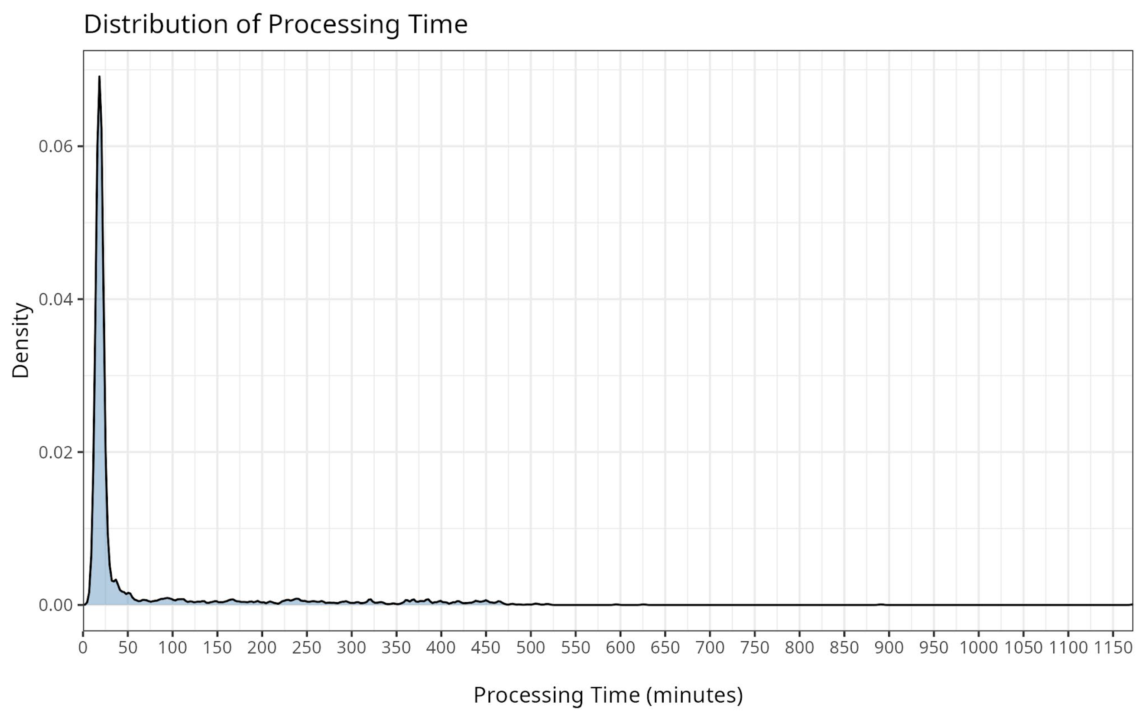
Figure 2. Aggregated system performance metrics across key anatomical sites in the two centres. DSC = Dice Similarity Coefficient, DJC = Dice Jaccard Coefficient, HD.95 = 95th percentile of the Hausdorff distance, Surface DSC = Surface Dice Similarity Coefficient, Over MDC = Over contouring, mean distance to conformity, Under MDC = Undercontouring mean distance to conformity.

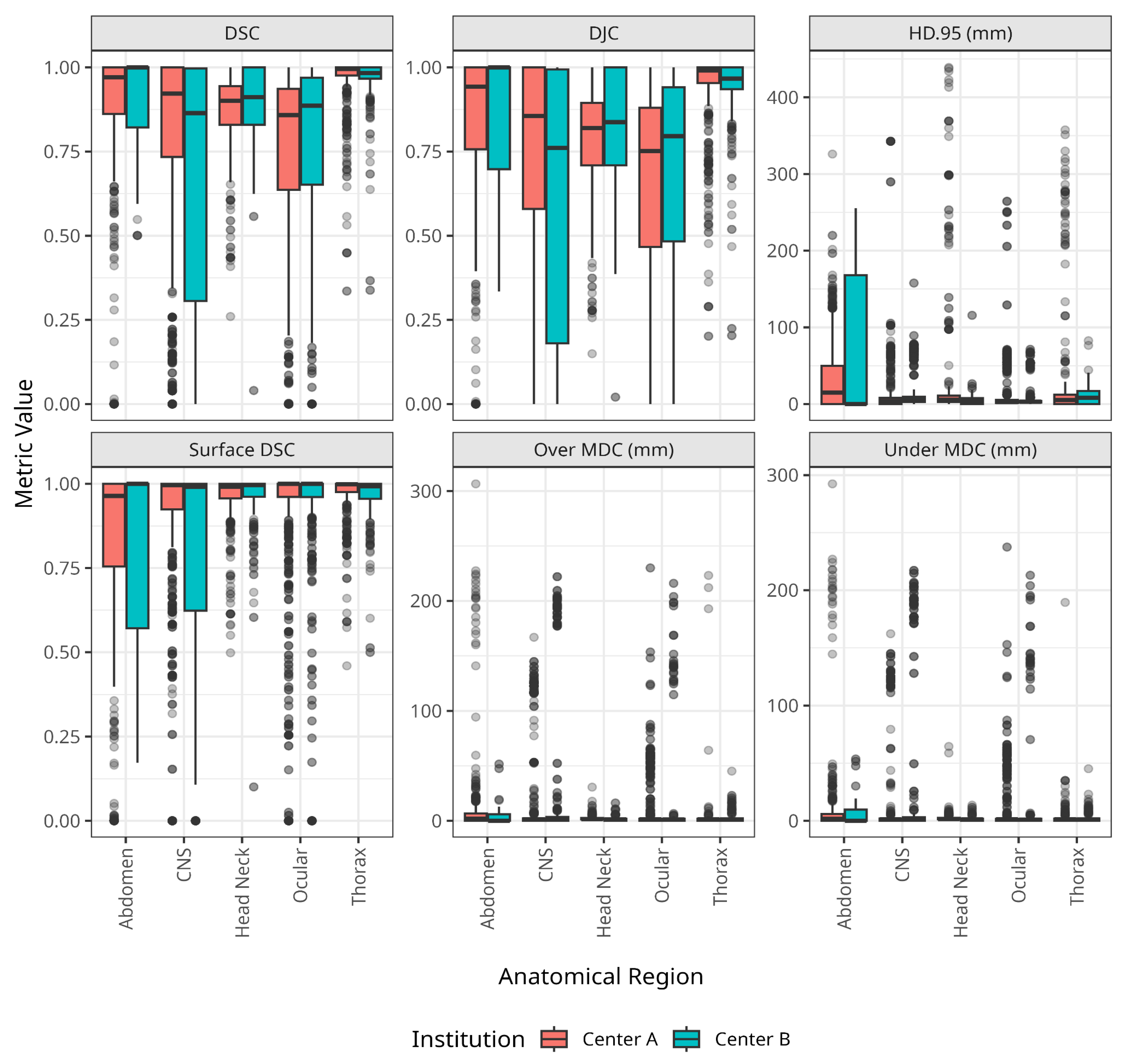
Table 1. Demographic characteristics and cancer site distribution of patients selected for quantitative spatial metrics evaluation, based on the selection criteria described in the methodology. * CT data of 11 breast patients could not be exported from Centre B for evaluation.

Parameter	Summary Measure	Overall (N = 380)	Centre A (N = 280 )	Centre B (N = 100)
Age	Mean (SD)	59 (14)	59 (15)	57 (13)
Gender	Male (%)	195 (51%)	150 (54%)	45 (45%)
Gender	Female (%)	185 (49%)	130 (46%)	55 (55%)
Cancer site	Breast	71 (19%)	40 (14%)	31 (31%)*
	Head Neck	80 (21%)	40 (14%)	40 (40%)
	Lung	52 (14%)	40 (14%)	12 (12%)
	Brain	40 (11%)	40 (14%)	0 (0%)
	Prostate	42 (11%)	40 (14%)	2 (2%)
	Cervix	49 (13%)	40 (14%)	9 (9%)
	Rectum	44 (12%)	40 (14%)	4 (4%)
	Bladder	2 (0.5%)	0 (0%)	2 (2%)

Table 2. Comparison of the aggregated spatial overlap metrics between centres. DSC = Dice Similarity Coefficient, DJC = Dice Jaccard Coefficient, HD.95 = 95th percentile of the Hausdorff distance, Surface DSC = Surface Dice Similarity Coefficient, Over MDC = Overcontouring, mean distance to conformity, Under MDC = Undercontouring mean distance to conformity, SD = standard deviation.

Parameter	Mean (SD) Centre A	Mean (SD) Centre B	p-value
DSC	0.81 (0.28)	0.78 (0.31)	<0.001
DJC	0.75 (0.30)	0.72 (0.33)	<0.001
Surface DSC	0.89 (0.26)	0.86 (0.28)	0.002
HD.95	20 (51)	15 (37)	<0.001
Over MDC	8 (30)	13 (49)	<0.001
Under MDC	8 (30)	12 (48)	<0.001

Table 3. Showing the frequencies and proportions of structures with major and minor modifications reported by Centre B for structures belonging to different cancer sites.

Parameter	Overall	No Modifications	Minor modifications	Major modifications
Head & Neck	400 (100%)	138 (34%)	116 (29%)	146 (36%)
Breast	99 (100%)	62 (63%)	28 (28%)	9 (9%)
Lung	22 (100%)	0 (0%)	12 (55%)	10 (45%)
Rectum	30 (100%)	2 (7%)	13 (43%)	15 (50%)

Disclaimer/Publisher’s Note: The statements, opinions and data contained in all publications are solely those of the individual author(s) and contributor(s) and not of MDPI and/or the editor(s). MDPI and/or the editor(s) disclaim responsibility for any injury to people or property resulting from any ideas, methods, instructions or products referred to in the content.

Copyright: This open access article is published under a Creative Commons CC BY 4.0 license, which permit the free download, distribution, and reuse, provided that the author and preprint are cited in any reuse.