

Submitted:
23 July 2026
Posted:
24 July 2026
You are already at the latest version
Abstract
Groundwater is an essential source of irrigation water in Mediterranean agricultural regions, where seasonal crop water requirements and recurrent drought increase pressure on shallow aquifers. Forecasting groundwater depth can help irrigators and water managers anticipate changes in pumping conditions and identify periods of increased abstraction risk. This study presents a data-driven framework for forecasting groundwater depth in the Tagus Nitrate Vulnerable Zone, central Portugal, an intensively cultivated region substantially dependent on shallow alluvial groundwater. The framework combines an autoregressive model with exogenous inputs and extreme gradient boosting and applies a leakage-safe rolling-origin validation strategy. Groundwater depth was modelled independently at each monitoring well using monthly observations, accounting for data gaps and uneven record lengths. Performance was assessed over forecast horizons of up to 12 months using error metrics calculated only from observed values. Feature-importance analysis showed the dominant role of groundwater persistence and seasonality, together with site-dependent contributions from precipitation, reference evapotranspiration, and river discharge. Forecast errors increased gradually with lead time but remained below 1 m for most wells. The framework provides forward-looking information that can complement irrigation-demand assessment and groundwater monitoring, supporting the anticipation of changing pumping conditions and the identification of areas requiring closer abstraction management.
Keywords:
groundwater irrigation
; agricultural water management
; alluvial aquifers
; groundwater depth forecasting
; machine learning
; mediterranean agriculture
1. Introduction
Groundwater is a critical component of water supply in Mediterranean agro-hydro-systems, where irrigation demand, climatic variability, and shallow aquifer conditions interact to create pronounced seasonal and interannual stress on water resources [1,2]. In many alluvial settings, groundwater bodies are characterised by high permeability, strong surface–groundwater connectivity, and limited storage buffering, resulting in water tables that respond rapidly to both hydroclimatic forcing and anthropogenic pressures [3,4]. These characteristics make alluvial aquifers particularly productive and suitable for irrigation supply, but also highly vulnerable to overexploitation and quality degradation under intensive agricultural use.
Within this context, nitrate vulnerable zones represent a regulatory and agricultural water-management priority across Europe [5]. Under the European Community Nitrates Directive (ND; Directive 91/676/EEC) [6], groundwater-monitoring networks [7] play a central role in assessing compliance, identifying trends, and supporting the design of mitigation measures. However, regulatory assessments remain largely retrospective, relying on historical analyses of groundwater levels and nitrate concentrations, with limited capacity to anticipate short- to medium-term dynamics. This constrains the ability of water authorities and agricultural water managers to respond proactively to emerging risks, particularly in systems subject to strong seasonal variability and increasing climate uncertainty [8,9,10].
From an agricultural water-management perspective, groundwater depth is both an indicator of aquifer status and an operational variable affecting irrigation access, pumping lift, energy requirements, and the adequacy of abstraction equipment. Forecasting groundwater depth can therefore complement retrospective trend analysis by helping irrigators and water managers anticipate drawdown, identify locations where pumping conditions may become less favourable, and prepare for periods when high crop water requirements coincide with declining groundwater levels. Such forecasts may also support abstraction planning, interpretation of groundwater-quality monitoring data, and the targeting of water-saving measures. Recent advances in data-driven modelling have shown that machine-learning methods can provide competitive groundwater-level and groundwater-depth forecasts, particularly when they exploit autoregressive persistence and incorporate hydroclimatic drivers [11,12,13].
Despite this progress, several challenges limit the operational uptake of machine-learning-based groundwater forecasting. First, predictive performance is often evaluated under experimental settings that do not reflect realistic operational use, for example through random train–test splits that introduce temporal leakage and lead to overly optimistic skill estimates [14]. Second, many studies focus on model architecture rather than on the end-to-end workflow, with limited attention to data acquisition, preprocessing, reproducibility, and integration with monitoring infrastructures [15,16]. Third, highly complex models such as deep neural networks, while powerful, can be difficult to interpret and maintain in institutional contexts where transparency, traceability, and robustness are essential requirements [13].
The use of groundwater forecasts in agriculture presents an additional challenge because irrigation requirements and aquifer status are often assessed through separate information streams. Crop water requirements are generally estimated from meteorological conditions, crop development, and soil-water availability, whereas groundwater status is commonly evaluated retrospectively from monitoring observations. This separation limits the capacity to anticipate situations in which high irrigation demand may coincide with unfavourable groundwater conditions. A forecasting framework capable of transforming existing monitoring records into well-specific, forward-looking information can help bridge this gap, particularly in regions where spatially and temporally complete records of agricultural groundwater abstraction are unavailable.
From an environmental-modelling perspective, these limitations highlight the need for forecasting approaches that balance predictive skill with interpretability, reproducibility, and operational feasibility. Autoregressive models with exogenous inputs (ARX) provide a conceptually transparent framework that aligns well with groundwater-system behaviour while allowing the integration of climatic and hydrological drivers [17]. When combined with modern nonlinear learners such as gradient-boosted decision trees, ARX formulations can capture complex relationships without requiring excessive data volumes [11,18].
Equally important is the embedding of such models within a structured and reproducible workflow. The Cross-Industry Standard Process for Data Mining (CRISP-DM) methodology offers a well-established framework for aligning modelling objectives with data preparation, model development, evaluation, and deployment and has been widely advocated for decision-support applications in environmental systems [19,20,24]. By emphasising traceability and iterative refinement, CRISP-DM supports the development of modelling pipelines that are transparent, maintainable, and suitable for operational use.
This study focuses on the Tagus Vulnerable Zone (TVZ), in central Portugal, an intensively cultivated agricultural region underlain by a shallow alluvial aquifer affected by interactions between agricultural land use, groundwater dynamics, and nitrate pollution risk [8]. The region combines long-term groundwater-monitoring records, marked seasonal forcing, and heterogeneous local conditions, making it a relevant test case for operational groundwater-depth forecasting in Mediterranean agro-hydro-systems [21,22,23]. The Tagus Alluvial Aquifer is an important source of irrigation water, although its spatial overlap with the underlying Tagus–Sado aquifer systems makes it difficult to assign abstractions unequivocally to a specific groundwater body. The current River Basin Management Plan reports a long-term mean annual recharge of 292.83 hm³ year⁻¹ but does not provide a directly comparable estimate of irrigation abstractions from the alluvial aquifer [25].
Within this context, the present study aims to develop and evaluate a reproducible, well-specific modelling workflow for groundwater-depth forecasting that can support the management of groundwater-dependent irrigation in a Mediterranean agricultural region. The framework integrates national groundwater-monitoring records with hydroclimatic drivers and applies a leakage-safe, data-driven forecasting protocol representative of operational conditions. The specific objectives are to:
integrate groundwater-monitoring and hydroclimatic data into a consistent, analysis-ready time-series dataset and characterise groundwater-depth behaviour across monitoring wells located in an intensively irrigated alluvial area;
implement a well-specific ARX–XGBoost forecasting framework for recursive multi-step prediction up to a 12-month horizon;
evaluate forecast performance using a leakage-safe rolling-origin protocol and assess model interpretability and robustness through feature-importance and horizon-dependent error analyses; and
discuss the operational relevance and limitations of groundwater-depth forecasts for supporting groundwater-dependent irrigation management.
By linking groundwater monitoring with the seasonal context of agricultural water use, this study contributes to the development of transparent and operational data-driven tools for groundwater-dependent irrigation management in vulnerable Mediterranean agricultural regions.
2. Materials and Methods
This study followed the CRISP-DM framework to structure the data science workflow [19,24]. This framework was adopted to ensure methodological transparency, traceability of decisions, and reproducibility, while aligning water management objectives with the development of the predictive modelling framework. The analysis combined computational tools for data extraction, transformation, and model implementation, complemented by visual analytics and Geographical Information Systems (GIS)-based inspection to facilitate data validation, exploratory analysis, and spatial coherence checks across the study area.
2.1. The Study Area
The study focused on the Tagus Vulnerable Zone, located in central Portugal within the lower Tagus River basin (Figure 1). The area is designated as vulnerable under the European Nitrates Directive (1991/676/ EEC; [6]), because of the susceptibility of groundwater to diffuse pollution from intensive agriculture [25]. The TVZ covers approximately 2,400 km², across the lower Tagus alluvial plain and, although defined administratively rather than by strict hydrological boundaries, lies roughly between 38.5°N - 39.0°N and 8.5°W - 9.5°W, within one of Portugal’s most intensively cultivated lowland regions.
The TVZ overlies two main hydrogeological units with contrasting characteristics. The Tagus Alluvial Aquifer, which is most relevant to this study, consists of Quaternary unconsolidated deposits associated with the Tagus River and its tributaries. These sediments are highly permeable and hydraulically connected to the river network, forming a shallow, unconfined groundwater system that responds rapidly to hydrological forcing [26]. Owing to its shallow depth and intensive agricultural land use, this aquifer is particularly vulnerable to nitrate leaching and irrigation return flows [8,25] and it constitutes an important groundwater supply source for irrigation in the region. The TVZ also includes the Left Bank Aquifer system, mainly composed of Tertiary formations along the margins of the Tagus valley. This aquifer is generally deeper and less directly connected to surface waters and constitutes an important source of potable water for human consumption in the region [8].
The regional climate is Mediterranean (Csa in the Köppen system) with hot, dry summers and mild, wet winters. Over a 30-year period, mean daily and maximum air temperatures are 13 and 29 ◦C, respectively. Mean annual precipitation ranges from about 700 to 900 mm, with recharge concentrated in winter and peak irrigation demand in summer [25]. This hydroclimatic regime causes marked seasonal groundwater-level fluctuations and contributes to long-term declines associated to irrigation withdrawals and climatic variability [8]. Climate change projections for the Mediterranean basin also indicate a reduction in rainfall together and a greater risk of summer drought [27,28,29].
The agricultural systems of the region have been intensified during the past decades, especially in the northern and central parts of the TVZ [8]. Currently the most representative crops are irrigated grain maize and horticulture for industrial processing (mainly tomatoes), followed by vineyards, olive groves and permanent pastures. The overall tendency in the northern part was for an increase of the irrigated area (by 16 %), which is an indicator of agriculture intensification and pressure upon the aquifers.
Groundwater depth monitoring in the TVZ is managed by the Portuguese Environment Agency (APA), within the national water resources monitoring framework supporting the designation, assessment, and periodic revision of Nitrate Vulnerable Zones under Council Directive 91/676/EEC. The network includes 69 groundwater wells distributed across the Alluvial and Left Bank aquifers, providing groundwater quantity and quality data. Given the closer linkage between the alluvial system and agricultural activity, this study focuses exclusively on the Tagus Alluvial Aquifer, the groundwater body most directly affected by agricultural practices and most relevant for operational groundwater depth forecasting in the TVZ.
2.2. Data Collection and First Step Pre-Processing
Groundwater depths (GWD, m) time series were obtained from National Water Resources Information System (SNIRH), which is an online platform that provides hydro-meteorological and water quality data from national monitoring networks [30]. Groundwater depths are recorded at irregular intervals and, in several cases, span multiple decades. As in other long-term monitoring networks, the data show uneven temporal coverage and gaps related to changes in monitoring practices and operational constraints. As part of the national monitoring system, these data are subject to quality control procedures, ensuring transparency, reproducibility, and suitability for scientific analysis and predictive modelling applications. To compile a large number of wells datasets in a consistent, analysis-ready format, SNIRH extraction was automated using a custom web-scraping routine that retrieved station pages, parsed tabular records, and exported harmonized CSV files for downstream processing. This approach avoided manual, station-by-station downloads and ensured consistent formatting across datasets, in line with recommendations for hydrologic information systems that emphasize programmatic access and standardized time-series export [16]. Daily river discharge (D, m3 s-1) was also retrieved from SNIRH for a hydrometric station within the Tagus system, providing a proxy for hydrological conditions and river–aquifer connectivity over 1973–2025. The use of Tagus River discharge is consistent with previous hydrological and estuarine modelling studies in the basin [31,32].
Precipitation (P, mm) and minimum and maximum air temperature (Tmin, Tmax, °C), were obtained from the European Observation Gridded Data Set (E-OBS) portal as gridded daily fields [33]. These data were extracted for the study region and assigned to the monitoring locations (145 spatial points in the present dataset), using freely available data products from the European Climate Assessment & Dataset (ECA&D) and the Copernicus Climate Data Store (ECA&D Project Team 2020).
Reference evapotranspiration (ETo, mm) was included as an indicator of atmospheric evaporative demand and of the seasonal pressure on irrigation requirements. In groundwater-dependent agricultural areas, higher ETo generally increases crop irrigation requirements and may consequently intensify groundwater abstraction, although the magnitude of this response depends on crop type, irrigated area, irrigation scheduling, system efficiency, and water availability. ETo should therefore be interpreted as a proxy for potential irrigation pressure rather than as a direct measurement of groundwater withdrawal. As complete meteorological data required for application of the Penman–Monteith method were not available, ETo was estimated using the Hargreaves–Samani empirical equation [34]:
where 0.0135 is a conversion factor to the International System of Units, Tmax and Tmin are daily maximum and minimum air temperatures (°C), KRS is the empirical radiation adjustment coefficient (0.15 from previous calibration for the region), Ra is solar radiation (MJ m-2 day-1), and 17.8 is an empirical coefficient related to the temperature scale.
Table 1 summarises all variables collected or calculated. These variables were temporally aligned with the groundwater depth time series.
Solar radiation was calculated from site latitude and day of year using standard astronomical relationships to represent seasonal variations in incoming radiation, following [35].
Groundwater depth at each monitoring well was organized as a time series, indexed by station identifier and year-month timestamp (ym). This representation was used consistently through the analysis. Well selection followed a multi-criteria approach based on: (i) adequate spatial representativeness of the Alluvial aquifer; (ii) sufficient temporal coverage to support robust model training; (iii) high data completeness and measurement consistency, minimising gaps and the need for extensive interpolation; and (iv) adequate data quality avoiding duplicated timestamps and implausible level fluctuations unrelated to hydroclimatic variability. These criteria are consistent with recent methodological guidance on groundwater monitoring network assessment and data quality evaluation [36,37].
Wells with extremely sparse observations, prolonged temporal discontinuities, or evident data quality issues were excluded. The final modelling set therefore included wells with no groundwater-depth gaps longer than three consecutive months and at least 50 monthly observations.
2.3. Exploratory Trend and Correlation Analysis
Trend analysis was used to characterize long-term behaviour and seasonality in the monthly groundwater depth series. Monotonic trends were first assessed using the non-parametric Mann–Kendall (MK) test, a rank-based method widely used for hydrological and hydrogeological time series because of its robustness to non-normality and low sensitivity to outliers [38,39]. To account for the marked seasonality of groundwater, the Seasonal Mann–Kendall (SMK) test was also applied, considering calendar months as seasons and combining within-month statistics across years to detect trends while accounting for recurring annual patterns [40]. For each series, two-sided p-values were reported to assess the statistical evidence for increasing or decreasing trend. Where trend magnitude was required, it was quantified using Sen’s slope estimator, defined as the median of pairwise slopes and robust to outliers [41]. Together, the Mann–Kendall and Seasonal Mann–Kendall tests, combined together with Sen’s slope estimator, enabled assessment of the presence, direction, and magnitude of monotonic trends in groundwater level time series.
A correlation analysis was performed using the Pearson correlation coefficient between GWD and the other variables. This analysis helped to identify which exogenous variables were most strongly associated with the target variable and could be included as predictors in the model. An exhaustive search over all possible predictor subsets was performed for final variable selection. This method used an efficient branch-and-bound algorithm and is implemented in the R package Leaps (https://CRAN.R-project.org/package=leaps).
2.4. Pre-Processing and Feature Engineering
Groundwater depth gaps in the selected well time series, limited to a maximum of three consecutive months, were filled using linear interpolation using the two adjacent months for which data was available. To link gridded climate data with point-based groundwater monitoring sites, each SNIRH well was georeferenced and matched to the nearest E-OBS grid cell. Daily time series for each climate variable was then extracted for each groundwater monitoring site. Daily hydroclimatic inputs were aggregated to monthly resolution to match the groundwater depth series time step. Precipitation was expressed as monthly totals, whereas temperature-based variables were summarized as monthly means. River discharge was also aggregated at monthly scale as a hydrological proxy. After temporal harmonization, missing values in the exogenous variables were filled by short-gap interpolation, followed where necessary by forward/backward filling, with the goal median used only as a final fallback. This procedure yielded a complete monthly predictor set for subsequent modelling [42].
2.5. Forecasting Model
Groundwater depth prediction was formulated as an autoregressive model with exogenous inputs, in which future groundwater depth at each monitoring well was estimated from its recent history and lagged hydroclimatic drivers. In this framework, the output at time t is expressed as a linear combination of past outputs and lagged exogenous inputs, plus a stochastic error term. ARX models are widely used in system identification and time-series forecasting because of their simplicity and interpretability [17,43]. Forecasting was performed to generate multi-step predictions over a 12-month horizon using a recursive (iterated) strategy (Figure 2).
2.5.1. Auto Regressive Model with Exogenous Variables
The groundwater depth of a well at time t (response variable, GWDt) was modelled as a function of its two previous values and a set of exogenous climatic, hydrological, and temporal variables. The exogenous variables included in the model (Equation 2), indexed by month t, were: Pt, precipitation; ETot, reference evapotranspiration; Dt, river discharge; Ct = cos(2πt/12); and St = sin(2πt/12), where Ct and St represent seasonality. In addition to contemporaneous values, on-month lags (t-1) of precipitation, reference evapotranspiration, and river discharge were also included.
One step-ahead forecasts were generated recursively over a 12-month horizon. For each well, the trained one step model was applied sequentially from horizon h=1 to h=12, with each predicted groundwater depth fed back to update the autoregressive inputs for the next step, so that predicted values progressively replaced observed values in the lag structure. This corresponds to the classical recursive multi-step forecasting strategy, in which a single one-step ahead model is iteratively applied and its outputs are reused as inputs for longer horizons [14,44].
The full model used to predict groundwater depth for the subsequent 12 months, that is, GWDt+1, GWDt+2, …, GWDt+12 is given below:
In these equations, f denotes the base single-step ARX forecasting model and ϵ a random error term. The asterisk indicates an estimated value. The one-month-ahead forecast depends only on observed values, whereas forecasts at longer horizons increasingly depend on previous estimates. Groundwater-depth estimates were obtained by recursively iterating the base model (f) while climatic and hydrologic predictors were the historical median for the corresponding month. This strategy was adopted to limit error propagation from exogenous-variable forecasts over the 12-month prediction horizon.
2.5.2. Model Training (XGBoost)
The simplest specification for the base model f in Equation 2 would be a linear autoregressive model. Instead, an XGBRegressor was adopted to capture non-linear relationships among the predictors for each well. XGBoost implements regularized gradient boosting of decision trees, and is widely used for tabular regression because of its high predictive performance and computational efficiency [18].
To ensure methodological consistency and comparability across locations, no automated hyper parameter tuning was performed. Instead, all wells were trained using the same fixed configuration: , , , , , with all remaining parameters kept as their library defaults. Model fitting used the standard squared error regression objective in XGBoost for continuous targets (objective = "reg:squarederror"), which minimises the squared difference between observed and predicted values, and is the default loss function for continuous regression targets in recent XGBoost releases.
2.5.3. Accuracy Assessment
Model performance was evaluated for each well over a 12 month hold-out period using the mean absolute error (MAE) and the root mean square error (RMSE) [45,46]. MAE is expressed in meters of groundwater depth and summarizes prediction accuracy as the average absolute difference between observed and predicted values. RMSE is expressed in meters of groundwater depth and summarizes prediction accuracy as the square root of the average squared difference between observed and predicted values.
Accuracy was assessed as follows. For a given well with a time series of n = 120 monthly observations (actual or interpolated), the base model was trained on months 1 to 108, and the full model (Equation 2) was used to predict GWD*109 to GWD*120. These predictions were compared with the test set, comprising observations GWD109 to GWD120. Prediction errors were computed as e1= GWD109 - GWD*109, …, e12= GWD120 - GWD*120, considering observed groundwater depths only; interpolated values in the test set were excluded. As this procedure yields at most one error estimate per forecast horizon, it was repeated k times by progressively removing the most recent k observations of the series.
For k=1, the model was trained on observations 1 to 107 and tested on observations 108 to 119, with observation 120 excluded. This procedure was repeated for successive values of k, generating a new set of error estimates at each iteration. The test set always comprised 12 observations, matching the forecast horizon, whereas the training set decreased progressively. A minimum length of 50 observations was imposed; thus, for a series of length n, the procedure was repeated m=n-12-50 times, yielding up to m non-interpolated estimates of the e1, ..., e12.
Mean error for each forecast horizon was calculated as the average of the corresponding error estimates, and the overall MAE was obtained as the mean across the 12 horizons. This rolling-origin forecasting preserves temporal order and mimics forecasting from a given information cut-off date [14,47].
Input data for each well were standardised using “scikit-learn.StandardScaler”. To prevent data leakage [48], the scaler was fitted only to the training set and then was applied to both the training and test data.
3. Results and Discussion
3.1. Data Availability and Trend Analysis
As defined in the Materials and Methods, the final modelling set included wells with no groundwater-depth gaps longer than three consecutive months and at least 50 observed values. Table 2 summarises the main characteristics of the 17 wells (presented in Figure 3) retained for forecasting, including the number of observed groundwater-depth values, well-specific completeness, overall MAE, and long-term trend descriptors. Completeness was defined as the proportion of time steps for which valid observations are available relative to the total number of expected observations. The selected wells showed substantial heterogeneity in record length and observational coverage, with the number of observations ranging from 51 to 233 and completeness, calculated within each well-specific observation window, ranging from 62.6% to 100.0%. This indicates that, despite the selection criteria applied, the modelling set still included wells with markedly different temporal support.
The selected wells showed substantial heterogeneity in record length and observational coverage, with the number of observations ranging from 51 to 233 and completeness, calculated within each well-specific observation window, ranging from 62.6% to 100.0%. This indicates that, despite the selection criteria applied, the modelling set still included wells with markedly different temporal support.
The long-term behaviour of groundwater depth at the 17 selected monitoring wells is summarised in Figure 4, which presents the results of the Mann–Kendall trend analysis together with Sen’s slope estimates. Figure 3 shows that monotonic trends were not spatially uniform across the monitoring network, with both increasing and decreasing trends detected among wells. This spatial heterogeneity is consistent with previous studies in Mediterranean alluvial aquifers, where local abstraction intensity, recharge conditions, and surface–groundwater connectivity lead to contrasting long-term responses within the same basin [1,21]. The magnitude of Sen’s slope values remains moderate overall, indicating gradual long-term evolution rather than abrupt regime shifts. Such behaviour is characteristic of groundwater systems in which long-term dynamics reflect cumulative recharge and abstraction processes acting over decadal timescales, while short-term variability is dominated by system persistence and storage effects [1,13]. Similar conclusions have been reported in groundwater time-series analyses across Europe, where strong persistence coexists with slow, spatially heterogeneous trends [11].
From an irrigation-management perspective, the coexistence of increasing, decreasing, and non-significant groundwater-depth trends indicates that groundwater conditions cannot be adequately represented by a single regional trajectory. Wells exhibiting significant increases in groundwater depth, corresponding to a deepening water table, may require particular attention where they are located in intensively irrigated areas, because persistent drawdown can progressively increase pumping lifts and reduce the operational margin of existing abstraction systems. However, the observed trends cannot be attributed directly to irrigation, as groundwater-depth records alone do not distinguish the effects of agricultural abstractions from those of recharge variability, river–aquifer interactions, or other local hydrogeological controls.
Figure 4 supports the adoption of well-specific forecasting models rather than a single pooled formulation. Differences in record length, temporal continuity, and observational support suggest that predictive relationships vary across locations. Studies comparing pooled and site-specific approaches have shown that localised models generally outperform regional formulations when groundwater dynamics are heterogeneous and monitoring records differ in length and quality [13,49,50].
3.2. Predictor Variables
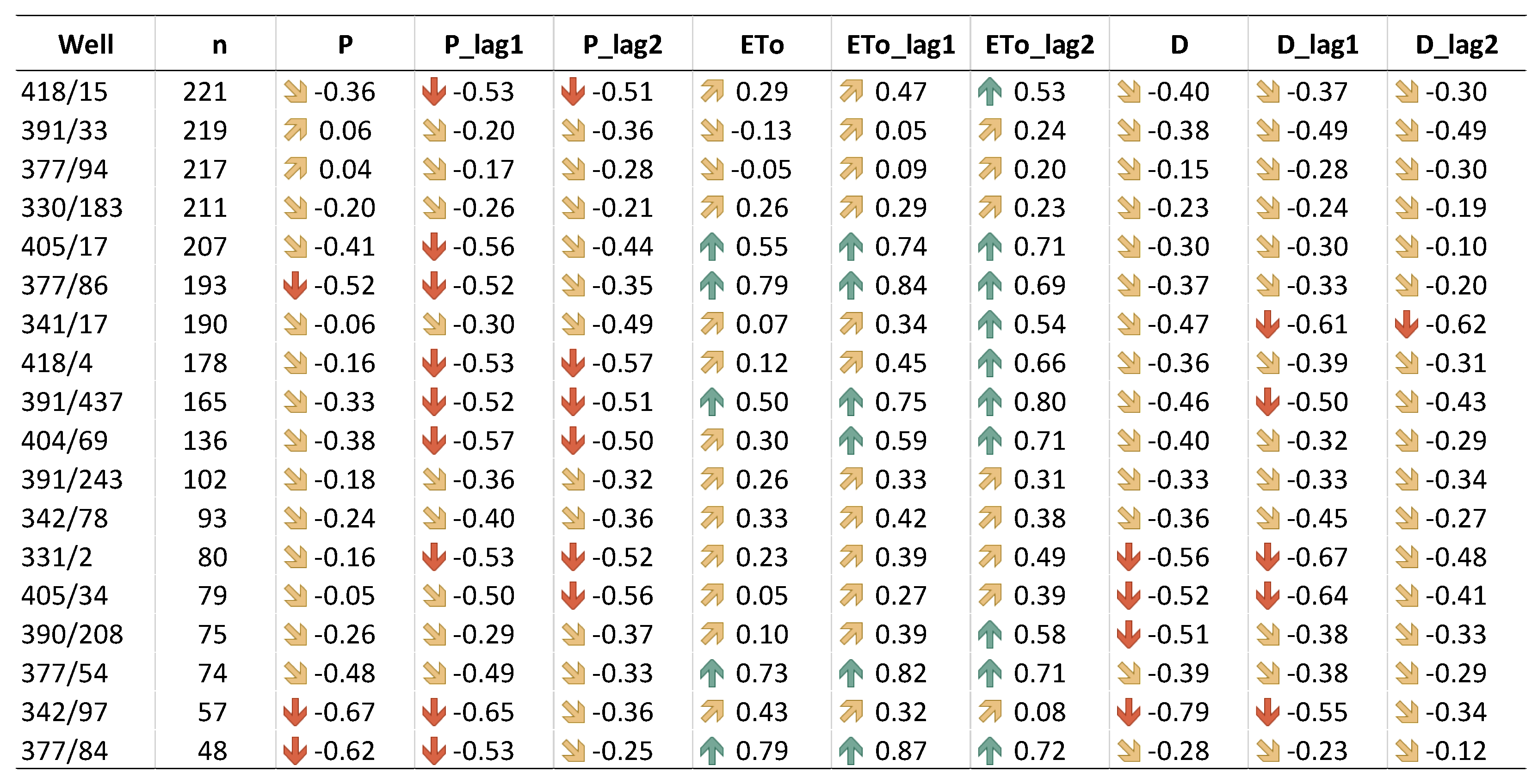
Table 3 shows, for each well, the number of original observations (before the time interpolations for short periods) and the correlation between GWD and each exogenous variable. Although the correlation values vary from well to well, GWD generally decreases with an increase in precipitation or river discharge and with a decrease in evapotranspiration. The effects of precipitation and evapotranspiration are often more pronounced for lagged variables.
Only the six lagged variables were considered for the selection of exogenous variables for the prediction model since the goal is to predict GWD based on past measurements. Depending on the well, the optimal number of predictor variables returned by package leaps ranged between two and six. However, when comparing the optimal adjusted-R2 with the adjusted-R2 of the complete linear model, only a small decrease was observed. The largest decrease in adjusted-R2 occurs for well 391/243, dropping from 0.205 with two variables to 0.181 with the complete model. These results justify including all six exogenous variables as predictors in the prediction model.
3.3. Model Validation
Model validation is illustrated in Figure 4 for three selected monitoring wells, chosen to represent the range of groundwater depth dynamics observed across the 17 wells. Well 331/2 shows no significant trend, high completeness, and no clear seasonality. Well 341/17 shows a significant trend and a long time series, but with only 69% completeness. Well 377/54 exhibits marked seasonality. The first three plots show the full time series (k=0, as defined in Section 2.5.3.), where the last 12 observations form the test set. The final plot shows the prediction for well 377/54 after discarding the most recent k = 25 observations. Together, these three wells reflect contrasting data patterns and provide a representative basis for evaluating model performance under different conditions.
For each well, the observed groundwater depth series is presented together with the predictions over the test window, with the start of the test period explicitly indicated. In these illustrative cases, the predictions closely follow the observed behaviour during the test period, reproducing both the direction and magnitude of groundwater depth changes.
Figure 5 shows that model performance differed not only among wells but also between the calibration and prediction periods. During calibration, the agreement between observed and predicted groundwater depth was strongest for Well 341/17 (R² = 0.954), indicating that the model was able to reproduce the dominant groundwater fluctuations at this site very satisfactorily. A reasonably good calibration was also obtained for Well 331/2 (R² = 0.799), whereas the markedly lower R² for Well 377/54 (R² = 0.678) points to a weaker representation of local groundwater dynamics. During the prediction period, performance declined in all wells, as expected, but the reduction was more pronounced for Well 377/54, where the higher RMSE and MAE values and the greater dispersion from the 1:1 line suggest limited predictive robustness. By contrast, Wells 331/2 and 341/17 maintained comparatively good predictive skill, with lower errors and a closer correspondence between simulated and observed values. Overall, these results indicate that the modelling framework is capable of capturing groundwater depth dynamics with acceptable reliability, although its transferability from calibration to prediction is clearly site-dependent and appears to be affected by local hydrogeological conditions that are not equally well represented in all wells.
Two factors explain the validation behaviour observed in this study. First, prediction error increases with forecast horizon (h = 1, …, 12), which is the expected behaviour of recursive multi-step forecasting. As lead time increases, each new prediction depends increasingly on previous predicted values, leading to progressive accumulation of uncertainty. Second, model performance is also affected by the rollback parameter (k). Increasing k shortens the available training series and reduces the amount of past information available to the model. As a result, the model has less temporal memory from which to learn groundwater dynamics.
These two effects are closely related. When k = 0, the model is trained on the full available time series and can better learn the temporal persistence of groundwater depth, which helps contain error growth as forecast horizon increases. By contrast, for larger k values, the shorter training series weakens the model’s representation of past behaviour, making it more difficult to maintain forecast accuracy at longer lead times.
This behaviour is consistent with the strong temporal persistence typical of groundwater systems, which has repeatedly been identified as a major source of predictive skill in data-driven groundwater forecasting [11,13]. Accordingly, the validation plots are consistent with previous studies showing that autoregressive formulations, including ARX-style models, often match or outperform purely exogenous approaches at short lead times because groundwater depth exhibits strong memory effects [13,51].
Figure 6 shows the variation in mean absolute error with the forecast horizon (h = 1, 2, ..., 12) for each analysed well. MAE was calculated using all rolling-origin windows (k = 0, 1, 2, …). In most wells, MAE remained below 1 m, indicating that the model captured temporal variability in groundwater depth with good predictive accuracy. Across forecast horizons, MAE generally increased with lead time, reflecting the cumulative uncertainty inherent to recursive multi-step forecasting. This pattern is documented in the forecasting literature and is expected when predicted values are iteratively reused as model inputs [14,44]. Importantly, the increase remained moderate and approximately linear across rolling-origin evaluations, indicating stable model behaviour and no error pronounced increase over the 12-month horizon. As described in Section 2.5.1, this behaviour was partly constrained by fixing climatic and hydrological predictors to historical monthly medians rather than forecasting them recursively.
Two wells showed a slightly different pattern. Well 342/78 had an average MAE of 1.45 m and was characterized by a relatively low number of observations (n=95), low completeness (68.3%), and a wide groundwater depth range (Table 2). Well 377/54 had an average MAE of 1.31 m and was associated with a short time series (n=77) and the largest groundwater depth range among all wells.
In terms of magnitude, the MAE values obtained here are comparable to those reported in recent studies on groundwater depth forecasting using machine-learning and hybrid approaches, despite differences in model structure and data availability. For example, [11,13] reported similar ranges of short- to medium-term forecast errors for autoregressive and neural-network-based models applied to groundwater monitoring data with strong temporal persistence.
3.4. Feature Relevance and Model Interpretability
Feature relevance across the 17 well-specific forecasting models is summarised in Figure 7, which presents a violin plot of normalised feature importance (gain, %) derived from the XGBoost models. Lagged groundwater depth variables consistently dominate feature importance across all wells, confirming the central role of autoregressive memory in groundwater depth forecasting. This pattern is consistent with previous studies showing that persistence explains a large share of groundwater-level variability, regardless of the modelling approach adopted [13,49,51].
ETo and the seasonal sine–cosine terms also showed consistently high importance, reflecting the strong seasonal control of atmospheric demand and annual periodicity on groundwater depth. This is consistent with the agricultural functioning of the study area. High atmospheric demand coincides with the main irrigation period and may be associated with increased groundwater withdrawals. However, because actual abstraction volumes were not included as model inputs, the importance of ETo should not be interpreted as a direct measure of irrigation effects. Instead, it captures a combination of seasonal climatic forcing, potential crop water demand, and recurrent management patterns embedded in the historical groundwater-depth response. This supports recent findings that explicit cyclical encoding improves model stability and interpretability in hydrological time-series forecasting [42,52,53].
3.5. Twelve-Month Groundwater Depth Forecasts
Operational groundwater depth forecasts for selected representative wells are presented in Figure 8, which shows the complete historical records together with 12-month ahead predictions generated from the most recent available observations. The forecasts are initiated at well-specific start dates, reflecting differences in data availability across the monitoring network, and are produced using the recursive ARX–XGBoost framework described above.
Across the wells shown, the forecasted trajectories exhibit smooth temporal evolution and remain consistent with the historical dynamics observed at each location. In particular, the models preserve the characteristic amplitude and timing of groundwater depth fluctuations, without producing unrealistic oscillations or abrupt divergences over the 12-month horizon. This behaviour is indicative of numerically stable recursive forecasting [14,44], a key requirement for operational groundwater applications.
Differences in forecasted behaviour between wells reflect the heterogeneity of groundwater dynamics across the monitoring network. Wells characterised by stronger seasonal variability display more pronounced forecasted fluctuations, whereas wells with smoother historical dynamics exhibit more gradual projected changes. Similar site-dependent forecast responses have been reported in groundwater forecasting studies using both classical time-series models and machine-learning approaches, highlighting that local system memory and variability strongly condition forecast behaviour [11,13].
Importantly, the forecasted groundwater depth trajectories remain within the range of historically observed values for all wells shown, suggesting that the models do not extrapolate beyond physically plausible bounds over the 12-month horizon. This contrasts with some deep-learning-based groundwater forecasting studies, where longer-horizon predictions can exhibit drift or loss of physical realism when recursive strategies are applied without adequate regularisation [12,13]. The conservative forecast behaviour observed here reflects the combined effect of autoregressive structure and the use of climatological representations for future exogenous inputs. From an operational perspective, these forecasts illustrate how the proposed modelling workflow can be used to generate forward-looking information for groundwater monitoring and management. While forecast uncertainty is expected to increase with lead-time, the ability to provide physically consistent 12-month projections represents a valuable complement to retrospective trend analysis, particularly in regulatory contexts where early warning of groundwater drawdown may support adaptive management actions [15].
3.6. Operational Relevance and Limitations for Groundwater-Dependent Irrigation
The practical relevance of groundwater-depth forecasting in irrigated agricultural areas arises from its relationship with pumping conditions and the seasonal concentration of water demand. In the Tagus Vulnerable Zone, peak irrigation requirements occur during late spring and summer, when precipitation and natural recharge are limited and atmospheric demand is high. Forecasts indicating an increase in groundwater depth during this period may therefore signal less favourable abstraction conditions, particularly in wells already characterised by marked seasonal fluctuations or long-term deepening trends.
The usefulness of the forecasts depends on the prediction horizon. Short-term forecasts, particularly at one-month lead time, may support operational decisions before or during the irrigation season by anticipating changes in pumping lift and identifying wells where groundwater access may become more demanding. Intermediate forecasts may contribute to irrigation-season planning, equipment inspection, and the early adoption of water-saving practices. Twelve-month forecasts are less suited to direct operational decisions because of their higher uncertainty, but they may still support strategic monitoring and the identification of locations requiring closer attention.
The well-specific modelling approach is particularly relevant in this context because groundwater responses were spatially heterogeneous. Differences in trends, seasonal behaviour, record completeness, and forecast accuracy indicate that aquifer conditions cannot be represented adequately by a single regional trajectory. Local forecasts may therefore provide more useful information than aquifer-wide averages, especially in areas where abstraction pressure, hydrogeological conditions, and surface–groundwater interactions vary over short distances.
Nevertheless, the forecasts should not be interpreted as direct estimates of groundwater availability, abstraction volumes, aquifer storage, or sustainable yield. The model does not explicitly include crop type, irrigated area, irrigation requirements, measured groundwater withdrawals, pumping-system characteristics, or groundwater-quality indicators. As discussed in Section 3.4, reference evapotranspiration represents atmospheric demand and may indirectly reflect seasonal irrigation pressure, but it does not quantify actual groundwater abstraction. Similarly, groundwater depth affects pumping lift but does not, on its own, quantify energy use or irrigation costs.
The proposed framework should therefore be regarded as an early-warning and monitoring component that can complement, rather than replace, irrigation water-balance assessments and hydrogeological analyses. Its operational value could be increased by integrating the forecasts with crop water requirements, soil-water status, irrigated land use, metered or estimated abstraction volumes, well characteristics, and pumping-energy information. Such integration would allow groundwater-depth forecasts to contribute more directly to decision-support systems for the coordinated management of irrigation demand and groundwater pressure in vulnerable Mediterranean agricultural regions.
4. Conclusions and Future Perspectives
This study shows that groundwater-depth forecasting can be successfully implemented under heterogeneous monitoring conditions using a workflow that remains operationally useful and physically interpretable. Beyond the predictive framework itself, a key contribution of this work is the compilation, harmonisation, and treatment of fragmented historical groundwater records, with time series ranging from six to 24 years. This effort transformed dispersed information into a consistent dataset suitable for analysis and modelling. The historical analysis revealed marked spatial variability in groundwater behaviour among wells, with approximately 29% exhibiting a statistically significant increase in groundwater depth, corresponding to a deepening water table. These results underline the importance of well-scale assessment for identifying localised changes and potentially vulnerable conditions. Lagged groundwater-depth terms were the most influential predictors, indicating that groundwater memory is the main driver of forecast performance, while seasonal and hydroclimatic variables provide complementary information. In most wells, errors remained below 1 m over the 12-month horizon, and predictions remained stable and hydrologically plausible despite the expected increase with lead time.
From an applied perspective, the proposed framework provides useful forward-looking information for groundwater users and managers. For farmers, short-term forecasts can help anticipate changes in groundwater depth and pumping lift, thereby supporting more informed irrigation planning. For water managers, the forecasts can help identify wells and periods requiring closer monitoring and further assessment. The framework should therefore be viewed primarily as a short- to medium-term decision-support tool rather than as a substitute for process-based simulation of aquifer behaviour. Future work should explore alternative forecasting architectures to reduce long-horizon error propagation and incorporate forecasted exogenous variables to better represent anomalous future conditions. Application to larger monitoring networks and other aquifers will be essential to assess transferability and robustness, while integration with crop water requirements, abstraction data, well characteristics, and pumping information could further enhance its practical relevance for groundwater-dependent irrigation management in vulnerable agricultural regions
Author Contributions
Conceptualization, Maria do Rosário Cameira; methodology, Manuel Campagnolo, Maria João Martins, João Rolim and Maria do Rosário Cameira; software, Diogo Pinto, Manuel Campagnolo, and Maria João Martins; validation: Diogo Pinto, João Rolim and Maria do Rosário Cameira; formal analysis, Diogo Pinto and Maria João Martins ; investigation, Diogo Pinto and Maria do Rosário Cameira.; resources, Maria do Rosário Cameira; data curation, Diogo Pinto; writing—original draft preparation, Diogo Pinto.; writing—review and editing, Maria do Rosário Cameira, João Rolim, Maria João Martins and Manuel Campagnolo; visualization, Diogo Pinto; supervision, Maria do Rosário Cameira, João Rolim, Manuel Campagnolo; project administration, Maria do Rosário Cameira; funding acquisition, Maria do Rosário Cameira. All authors have read and agreed to the published version of the manuscript.”.
Funding
This research was funded by the CLEPSYDRA project “Groundwater monitoring and Decision Support System development to optimize decision making in sensitive and water-scarce agricultural environments in the Mediterranean context” grant number Euro_MED0200626. This work was also supported by FCT – Fundação para a Ciência e a Tecnologia, I.P., through the projects UIDB/04129/2020 of LEAF-Linking Landscape, Environment, Agriculture and Food - Research Unit; UID/00239/2025 and UID/PRR/00239/2025 of the Forest Research Centre, and LA/P/0092/2020 of the Associate Laboratory TERRA. The funders had no role in the design of the study; in the collection, analyses, or interpretation of data; in the writing of the manuscript; or in the decision to publish the results.
Data Availability Statement
Data will be provided upon request.
Conflicts of Interest
The authors declare no conflicts of interest.
Abbreviations
The following abbreviations are used in this manuscript:
| APA | Portuguese Environment Agency |
| ARX | Autoregressive model with exogenous inputs |
| CRISP-DM | Cross-Industry Standard Process for Data Mining |
| e1, …, e12 | Forecast errors at each prediction horizon |
| EC | European Community |
| ECA&D | European Climate Assessment & Dataset |
| E-OBS | European Observation gridded dataset |
| f | Base single-step forecasting model |
| GIS | Geographic Information System |
| GWD | Groundwater depth |
| MAE | Mean Absolute Error |
| MK | Mann–Kendall |
| ND | Nitrates Directive |
| RMSE | Root mean square error |
| SMK | Seasonal Mann–Kendall |
| SNIRH | National Water Resources Information System |
| TVZ | Tagus Vulnerable Zone |
| XGBoost | Extreme Gradient Boosting |
| α | Significance level |
| ɛ | Random error term |
The following symbols are used in this manuscript:
| Ct | Cosine seasonal term, cos(2πt/12) |
| Dt | River discharge at month t (m³ s⁻¹) |
| ETot | Reference evapotranspiration at month t |
| GWD*t | Estimated groundwater depth at time t (m) |
| GWDt | Groundwater depth at time t (m) |
| h | Forecast horizon |
| k | Rollback step in rolling-origin validation |
| KRS | Empirical radiation adjustment coefficient |
| Lag 1 | One month before |
| Lag 2 | Two months before |
| M | Number of rolling-origin iterations |
| N | Length of the time series |
| nobs | Number of observed groundwater-depth values |
| Pt | Precipitation at month t (mm) |
| Ra | Solar radiation (MJ m⁻² day⁻¹) |
| St | Sine seasonal term, sin(2πt/12) |
| t | Time index |
| Tmax | Daily maximum air temperature (°C) |
| Tmin | Daily minimum air temperature (°C) |
| ym | Year–month timestamp |
References
- Custodio, E. Aquifer overexploitation: what does it mean? Hydrogeology Journal 2002, 10. [CrossRef]
- Döll, P.; Müller Schmied, H.; Schuh, C.; Portmann, F.T.; Eicker, A. Global-scale assessment of groundwater depletion and related groundwater abstractions: Combining hydrological modeling with information from well observations and GRACE satellites. Water Resources Research 2014, 50(7), 5698–5720. [CrossRef]
- Baird, A.J.; Low, R.G. The water table: Its conceptual basis, its measurement and its usefulness as a hydrological variable. Hydrological Processes 2022, 36(6). [CrossRef]
- Kalbus, E.; Reinstorf, F.; Schirmer, M. Measuring methods for groundwater–surface water interactions: A review. Hydrology and Earth System Sciences 2006, 10(6), 873–887. [CrossRef]
- Serra, J.; Marques-dos-Santos, C.; Marinheiro, J.; Cruz, S.; Cameira, M.R.; De Vries, W.; Garnier, J. Assessing nitrate groundwater hotspots in Europe reveals an inadequate designation of Nitrate Vulnerable Zones. Chemosphere 2024, 355. [CrossRef]
- Council Directive 91/676/EEC of 12 December 1991 concerning the protection of waters against pollution caused by nitrates from agricultural sources. Official Journal of the European Communities 1991, 34, 1-8.
- Koreimann, C.; Grath, J.; Winkler, G.; Nagy, W.; Vogel, W.R. Groundwater monitoring in Europe; European Environment Agency: Copenhagen, Denmark, 1996.
- Cameira; M.R.; Rolim, J.; Valente, F.; Mesquita, M.; Dragosits, U.; Cordovil, C.M. Translating the agricultural N surplus hazard into groundwater pollution risk: Implications for effectiveness of mitigation measures in nitrate vulnerable zones. Agriculture, Ecosystems & Environment 2021, 306. [CrossRef]
- Dhapre, M.; Jadhav, S.; Das, D.; Khan, J.; Kim, Y.; Chiao, S.; Danielson, T. A systematic review of machine learning in groundwater monitoring. Environmental Modelling & Software 2025, 192. [CrossRef]
- Stigter, T.Y.; Miller, J.; Chen, J.; Re, V. Groundwater and climate change: threats and opportunities. Hydrogeology Journal 2023, 31(1), 7-10. [CrossRef]
- Brakenhoff, D.A.; Vonk, M.A.; Collenteur, R.A.; Van Baar, M.; Bakker, M. Application of time series analysis to estimate drawdown from multiple well fields. Frontiers in Earth Science 2022, 10. [CrossRef]
- Lin, H.; Gharehbaghi, A.; Zhang, Q.; Band, S.S.; Pai, H.T.; Chau, K.W.; Mosavi, A. Time series-based groundwater level forecasting using gated recurrent unit deep neural networks. Engineering Applications of Computational Fluid Mechanics 2022, 16(1), 1655-1672. [CrossRef]
- Wunsch, A.; Liesch, T.; Broda, S. Groundwater level forecasting with artificial neural networks: a comparison of long short-term memory (LSTM), convolutional neural networks (CNNs), and non-linear autoregressive networks with exogenous input (NARX). Hydrology and Earth System Sciences 2021, 25(3), 1671-1687. [CrossRef]
- Hyndman, R.J.; Athanasopoulos, G. Forecasting: Principles and Practice, 2nd ed.; OTexts: Melbourne, Australia, 2018. Available on-line: https://otexts.com/fpp2/ (accessed on 14/03/2026).
- Aguilera, H.; Guardiola-Albert, C.; Naranjo-Fernández, N.; Kohfahl, C. Towards flexible groundwater-level prediction for adaptive water management: using Facebook’s Prophet forecasting approach. Hydrological Sciences Journal 2019, 64(12), 1504–1518. [CrossRef]
- Jones, A.S.; Horsburgh, J.S. Hydrologic information systems: An introductory overview. Environmental Modelling & Software 2025, 185. [CrossRef]
- Ljung, L. System identification: Theory for the user, 2nd ed.; PTR Prentice Hall: Englewood Cliffs, New Jersey.
- Chen, T.; Guestrin, C. XGBoost: A scalable tree boosting system. In Proceedings of the 22nd ACM SIGKDD International Conference on Knowledge Discovery and Data Mining, San Francisco, United States of America, 13-17/08/2016. [CrossRef]
- Shearer, C. The CRISP-DM model: The new blueprint for data mining. Journal of Data Warehousing 2000, 5(4), 13–22.
- Wirth, R.; Hipp, J. CRISP-DM: Towards a standard process model for data mining. In Proceedings of the 4th International Conference on the Practical Applications of Knowledge Discovery and Data Mining, Manchester, England, 11-13/04/2000.
- Costa, D.; Santos, J.; Chambel, A. Five decades of groundwater change across a diverse Mediterranean climate region: Disentangling natural and human drivers of water quantity and quality. Science of the Total Environment 2025, 1006. [CrossRef]
- Galdelli, A.; Fronzi, D.; Narang, G.; Mancini, A.; Tazioli, A. Groundwater level forecasting using data-driven models and vadose zone: A comparative analysis of ARIMA, SARIMAX, Prophet, and NeuralProphet. Applied Computing and Geosciences 2025, 28. [CrossRef]
- Gelati, E.; Zajac, Z; Ceglar, A.; Bassu, S.; Bisselink, B.; Adamovic, M.; Bernhard, J.; Malagó, A.; Pastori, M.; Bouraoui, F.; de Roo, A. Assessing groundwater irrigation sustainability in the Euro-Mediterranean region with an integrated agro-hydrologic model. Advances in Science and Research 2020, 17, 227-253. [CrossRef]
- Chapman, P.; Clinton, J.; Kerber, R.; Khabaza, T.; Reinartz, T.; Shearer, C.; Wirth, R. CRISP-DM 1.0: Step-by-step data mining guide. SPSS inc 2000, 9(13), 1-73.
- APA. Plano de Gestão de Região Hidrográfica. Região hidrográfica do Tejo e Ribeiras do Oeste (RH5) 2016. Lisboa, Portugal.
- Almeida, C.; Lopo, M.; Jesus, M.; Gomes, A. Sistemas Aquíferos de Portugal. Centro de Geologia da Universidade de Lisboa: Lisbon, Portugal; Instituto Nacional da Água, Portugal: Lisboa, Portugal. 2000. [CrossRef]
- Cardoso, R.M.; Soares, P.M.M.; Lima, D.C.A.; Miranda, P.M.A. Mean and extreme temperatures in a warming climate: EURO CORDEX and WRF regional climate high resolution projections for Portugal. Climate Dynamics 2019, 52, 129–157. [CrossRef]
- Giorgi, F.; Lionell, P. Climate change projections for the Mediterranean region. Global and Planetary Change 2008, 63(2-3), 90-104. [CrossRef]
- Soares, P.M.M.; Cardoso, R.M.; Lima, D.C.A.; Miranda, P.M.A. Future precipitation in Portugal: high-resolution projections using WRF model and EUROCORDEX multi-model ensembles. Climate Dynamics 2017, 49, 2503–2530. [CrossRef]
- Sistema Nacional de Informação de Recursos Hídricos (SNIRH). Available on-line: https://apambiente.pt/agua/sistema-nacional-de-informacao-de-recursos-hidricos-snirh (accessed on 14/03/ 2026).
- Fortunato, A.B.; Freire, P.; Rilo, A.; Viseu, T.; Rodrigues, M. Mapping inundation of estuarine margins driven by ocean and fluvial forcings. In Proceedings of the 8th IAHR Europe Congress, Lisbon, Portugal, 4-7/06/2024.
- Dias, L.F.; Santos, F.; Carvalho, S.; Nunes, J.P.; Lima, D.; Cardoso, R.; Bento, V.; Rodrigues, M.; Matos Soares, P.; Santos, F.D. RNA2100 – Sectoral Impacts Modelling - Hydrological Balance & Agroforestry - Portugal Mainland. Agência Portuguesa do Ambiente: Lisbon, Portugal.
- Cornes, R.C.; Van Der Schrier, G.; Van Den Besselaar, E.J.; Jones, P.D. An ensemble version of the E-OBS temperature and precipitation data sets. Journal of Geophysical Research: Atmospheres 2018, 123(17), 9391-9409. [CrossRef]
- Hargreaves, G.H.; Samani, Z.A. Estimating potential evapotranspiration. Journal of the irrigation and Drainage Division 1982, 108(3), 225-230. [CrossRef]
- Allen, R.G.; Pereira, L.S.; Raes, D.; Smith, M. Crop Evapotranspiration-Guidelines for computing crop water requirements. FAO Irrigation and drainage paper 56 1998, 300(9). https://www.fao.org/4/x0490e/x0490e00.htm.
- Bosserelle, A.L.; Hughes, M.W. Groundwater monitoring infrastructure: Evaluation of the shallow urban and coastal network in Ōtautahi Christchurch. Journal of Hydrology: Regional Studies 2024, 55. [CrossRef]
- Evaluating groundwater monitoring data (Deliverable D5.2). Available on-line: https://repository.europe-geology.eu/egdidocs/hover/hover+d5_2+final+evaluating+groundwater+monitoring.pdf (14/03/2026).
- Mann, H.B. Nonparametric tests against trend. Econometrica 1945, 13(3), 245–259.
- Yue, S.; Pilon, P.; Phinney, B.; Cavadias, G. The influence of autocorrelation on the ability to detect trend in hydrological series. Hydrological Processes 2002, 16(9), 1807–1829. [CrossRef]
- Hirsch, R.M.; Slack, J.R. A nonparametric trend test for seasonal data with serial dependence. Water Resources Research 1984, 20(6), 727–732. [CrossRef]
- Sen, P.K. Estimates of the regression coefficient based on Kendall’s tau. Journal of the American Statistical Association 1968, 63(324), 1379–1389. [CrossRef]
- Bleidorn, M.T.; Pinto, W.P.; Schmidt, I.M.; Mendonça, A.S.F.; Reis, J.A.T. Methodological approaches for imputing missing data into monthly riverflow time series. Revista Ambiente & Água 2022, 17(2). [CrossRef]
- ARX timeseries model. Available on-line:. https://apmonitor.com/dde/index.php/Main/AutoRegressive (accessed on 14/03/2026).
- Taieb, S.B.; Hyndman, R. Boosting multi-step autoregressive forecasts. In Proceedings of the 31st International Conference on Machine Learning, Beijing, China, 21-26/06/2014.
- Regression evaluation metrics. Available on-line: https://apxml.com/courses/getting-started-with-scikit-learn/chapter-2-supervised-learning-regression/regression-evaluation-metrics (accessed on 14/03/2026).
- 3.4. Metrics and scoring: Quantifying the quality of predictions. Available on-line: https://scikit-learn.org/stable/modules/model_evaluation.html (accessed on 14/03/2026).
- Bergmeir, C.; Hyndman, R.J.; Koo, B. A note on the validity of cross-validation for evaluating autoregressive time series prediction. Computational Statistics & Data Analysis 2018, 120, 70-83. [CrossRef]
- 11. Common pitfalls and recommended practices. Available on-line: https://scikit-learn.org/stable/common_pitfalls.html (accessed on 14/03/2026).
- Alfio, M.R.; Pisinaras, V.; Panagopoulos, A.; Balacco, G. Groundwater level response to precipitation at the hydrological observatory of Pinios (central Greece). Groundwater for Sustainable Development 2024, 24. [CrossRef]
- Zhang, Y.; Li, H.; Zhong, Y.; Liu, W.; Chen, S.; Zhang, X.; Uddin, M.G.; Wang, Y.; Zhu, B.; Huang, X.; Wang, Y. Comparative assessment of machine-learning models for daily groundwater level prediction in a Metropolis, southwestern China. Journal of Hydrology: Regional Studies 2026, 64. [CrossRef]
- Chenjia, Z.; Xu, T.; Zhang, Y.; Ma, D. Deep learning models for groundwater level prediction based on delay penalty. Water Supply 2024, 24(2), 555-567. [CrossRef]
- Cyclical features in time series. Available on-line: https://skforecast.org/0.15.1/faq/cyclical-features-time-series.html (accessed on 14/03/2026).
- Recursive multistep forecasting. Available on-line: https://skforecast.org/0.15.1/user_guides/autoregresive-forecaster.html (accessed on 14/03/2026).
Figure 1.
Location of the Tagus Vulnerable Zone in continental Portugal, showing its spatial extent in relation to the Tagus Alluvial Aquifer and the Left Bank Aquifer.
Figure 1.
Location of the Tagus Vulnerable Zone in continental Portugal, showing its spatial extent in relation to the Tagus Alluvial Aquifer and the Left Bank Aquifer.
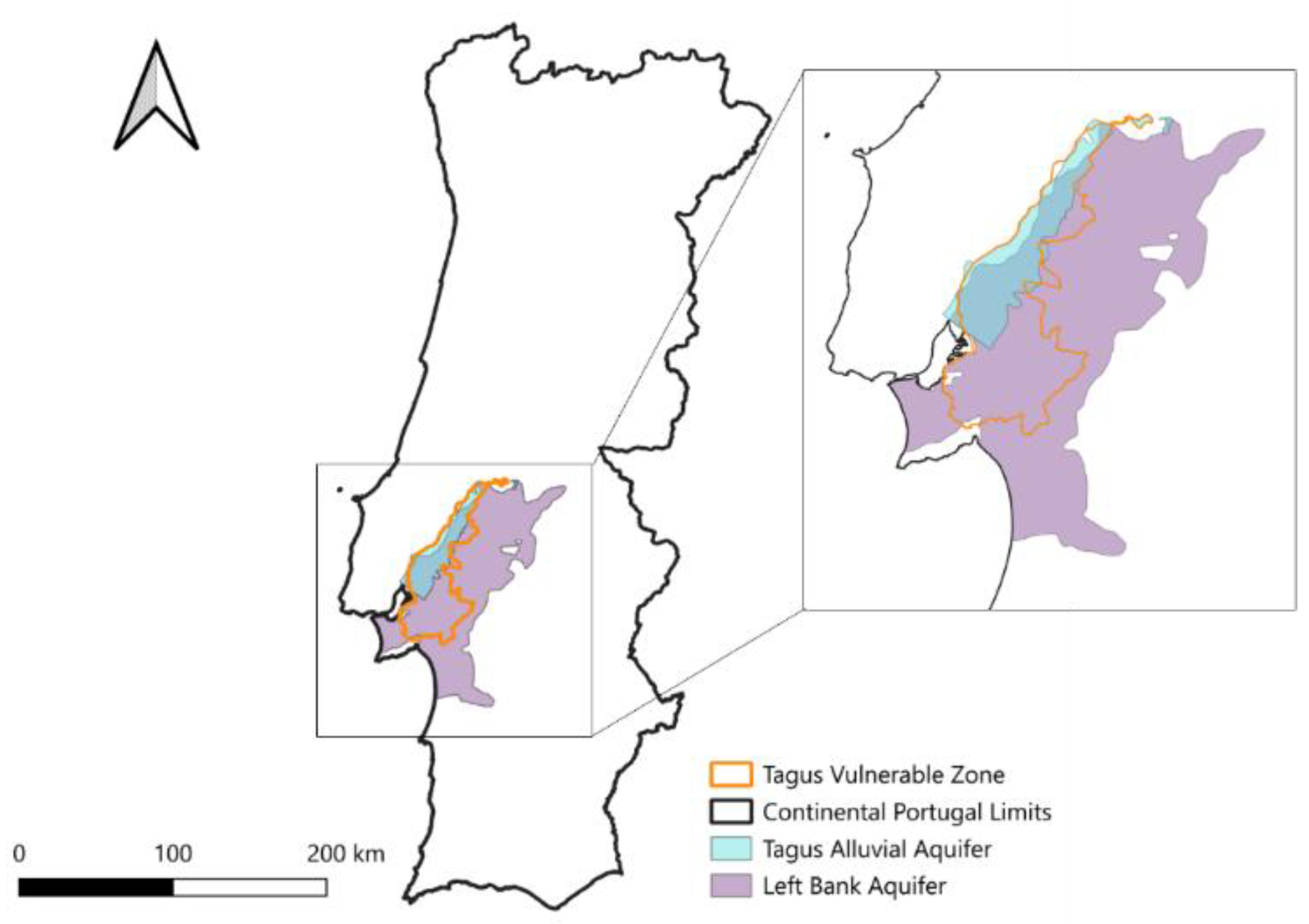
Figure 2.
Groundwater depth forecasting using ARX-XGBOST framework.
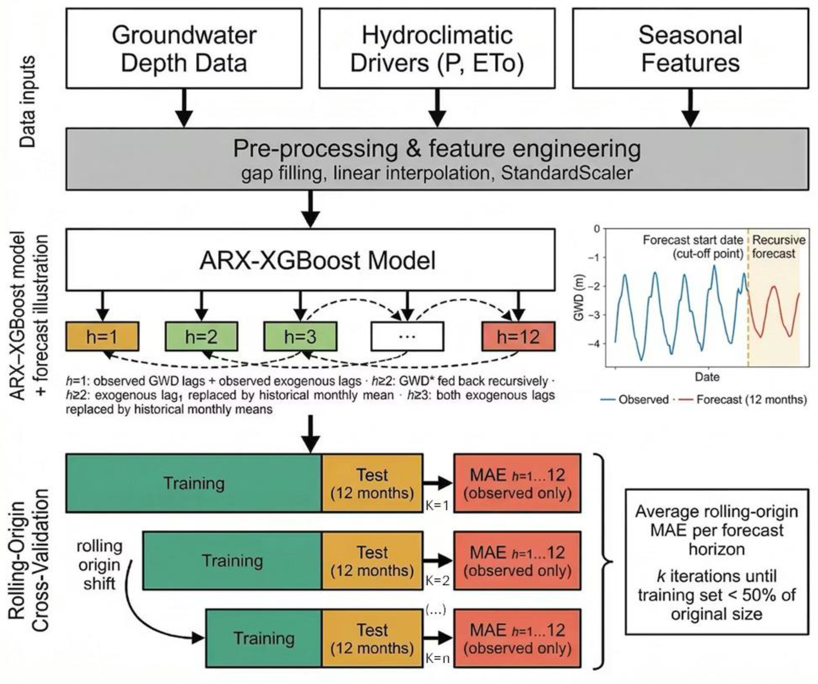
Figure 3.
Long-term trends in groundwater depth (y axis). The dashed line represents the trend estimated from the first observation. The well code is shown at the bottom right of each panel, followed by ‘-’ or ‘+’ when the trend is statistically significant (α=0.05).
Figure 3.
Long-term trends in groundwater depth (y axis). The dashed line represents the trend estimated from the first observation. The well code is shown at the bottom right of each panel, followed by ‘-’ or ‘+’ when the trend is statistically significant (α=0.05).
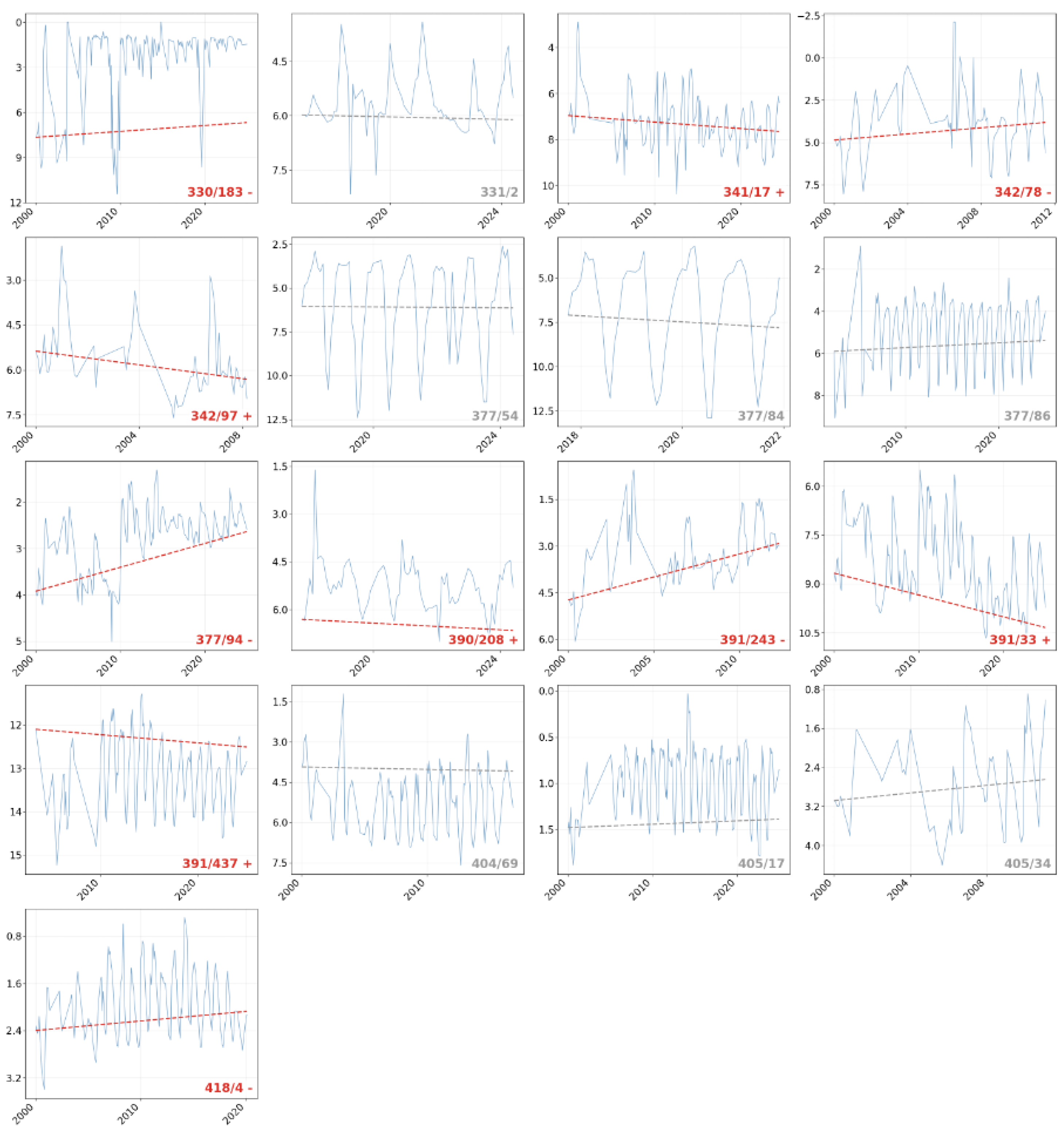
Figure 4.
Rolling-origin validation of groundwater depth forecasts for representative monitoring wells. k represents the number of months the forecasting origin has been rolled forward in the historical data.
Figure 4.
Rolling-origin validation of groundwater depth forecasts for representative monitoring wells. k represents the number of months the forecasting origin has been rolled forward in the historical data.
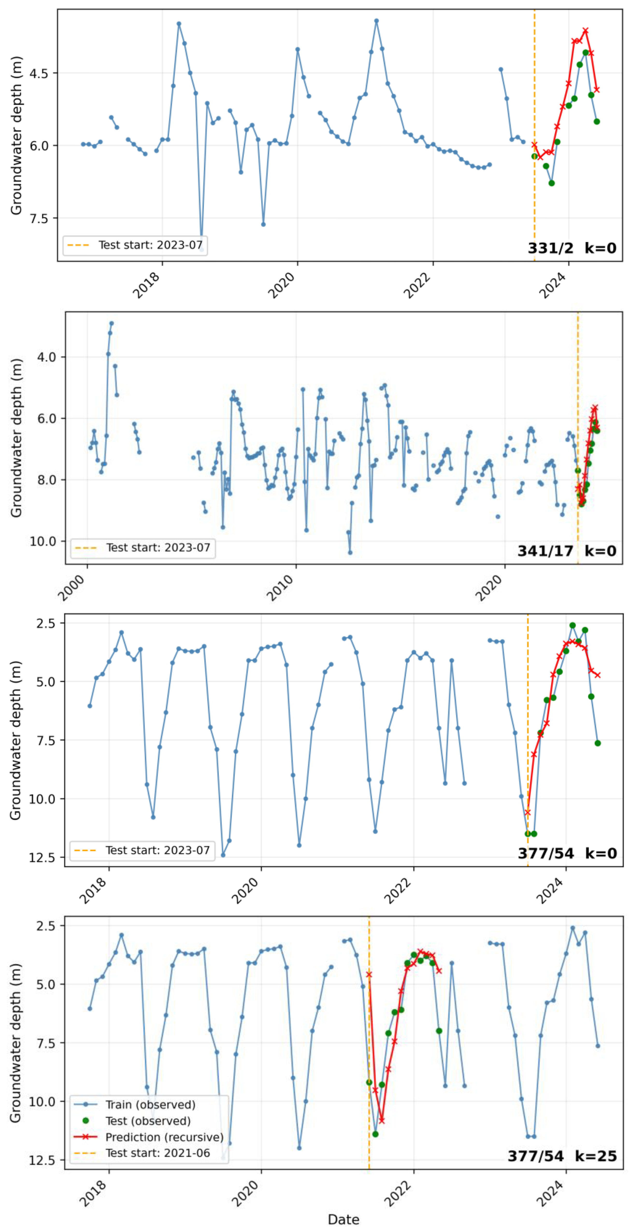
Figure 5.
Relation between predicted and observed groundwater depth for the calibration and validation phases for the representative monitoring wells.
Figure 5.
Relation between predicted and observed groundwater depth for the calibration and validation phases for the representative monitoring wells.
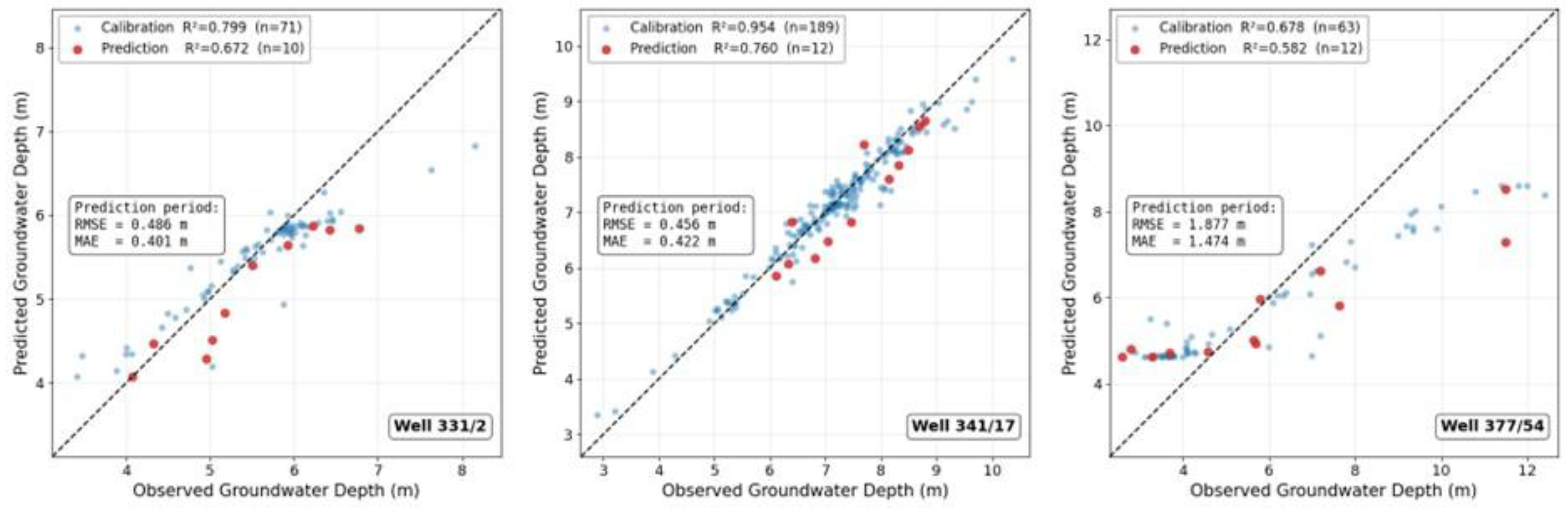
Figure 6.
Mean absolute error (MAE) by forecast horizon for all analysed wells.
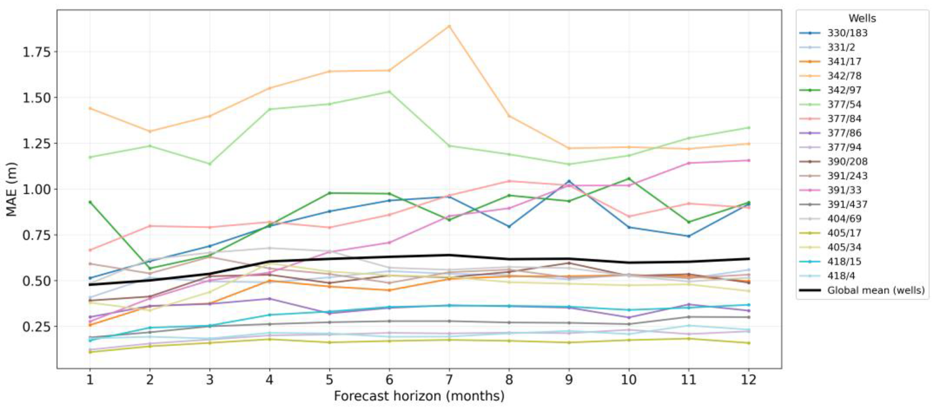
Figure 7.
Violin plot of normalised feature importance (gain, %) for the predictors included in the ARX–XGBoost groundwater-depth models, summarising their relative contribution across the 17 well-specific models.
Figure 7.
Violin plot of normalised feature importance (gain, %) for the predictors included in the ARX–XGBoost groundwater-depth models, summarising their relative contribution across the 17 well-specific models.
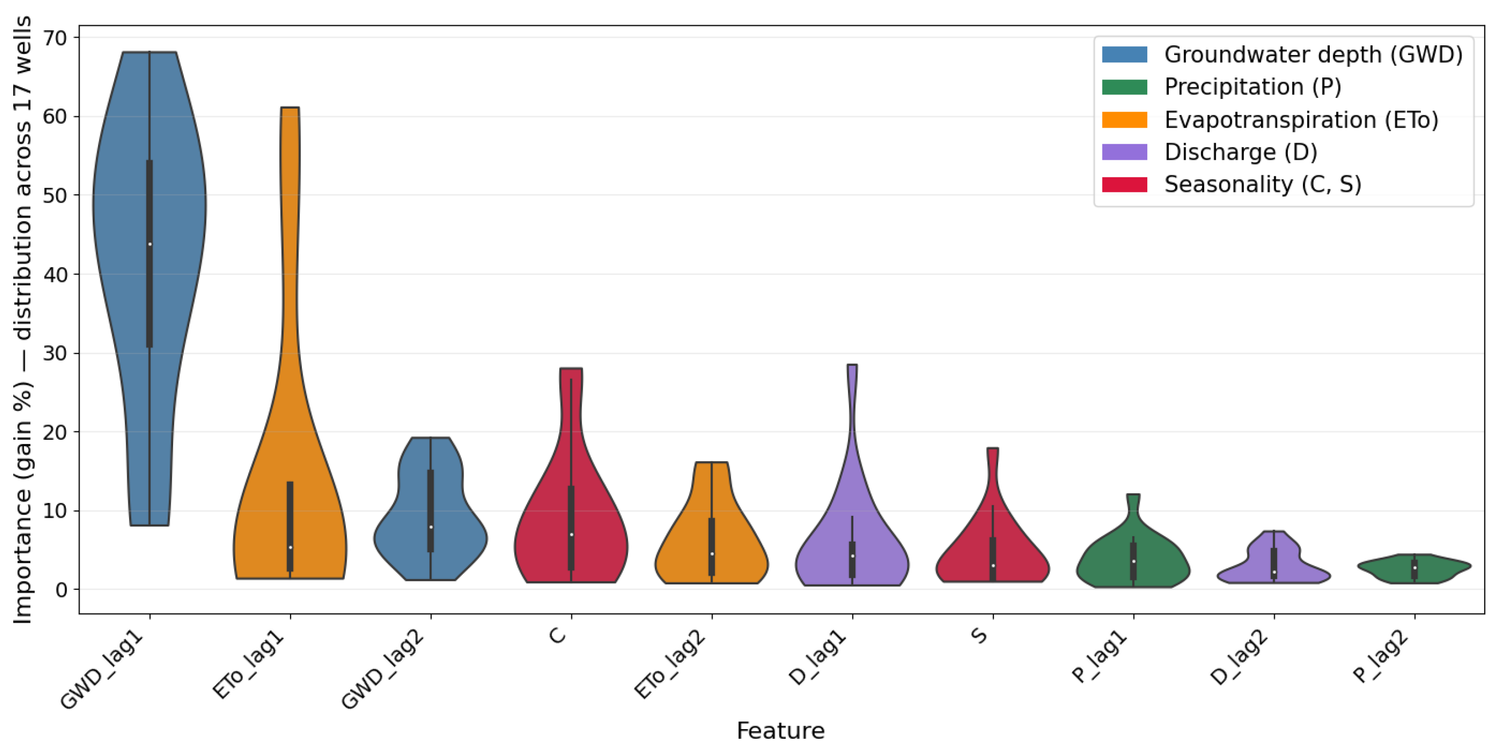
Figure 8.
Twelve-month groundwater depth forecasts for representative monitoring wells.
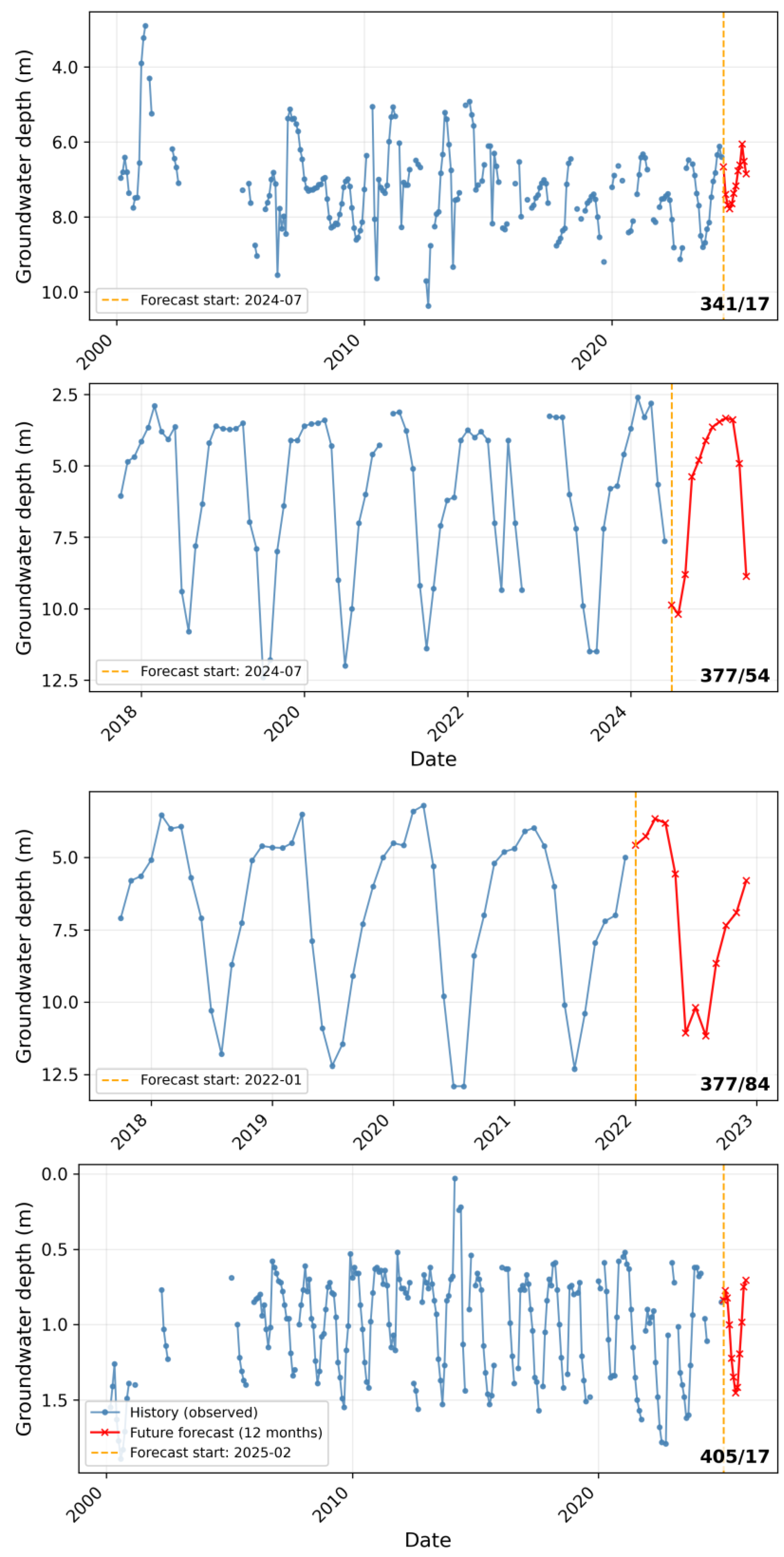

Table 1.
Summary of datasets and variables included in the database.
| Data type | Units | Source | Temporal coverage | Original temporal resolution | Number of spatial points |
|---|---|---|---|---|---|
| Groundwater depth | m | SNIRH | 1974-10-01 20205-01-16 |
Irregular (monthly/daily) | 69 |
| River discharge | m3 s-1 | SNIRH | 1973-10-02 2025-03-13 |
Daily | 1 |
| Maximum and minimum air temperature | º C | E-OBS | 2000-2024 | Daily | 145 |
| Precipitation | mm | E-OBS | 2000-2024 | Daily | 145 |
| Solar radiation | MJ m-2 d-1 | Calculated | 2000-2024 | Daily | 145 |
Table 2.
Summary of the 17 monitoring wells retained for forecasting, including the number of observed groundwater-depth values (nobs), well-specific completeness (%), overall mean absolute error, MAE (m), Sen’s slope (m yr⁻¹), and the sign of statistically significant monotonic trends (α=0.05).
Table 2.
Summary of the 17 monitoring wells retained for forecasting, including the number of observed groundwater-depth values (nobs), well-specific completeness (%), overall mean absolute error, MAE (m), Sen’s slope (m yr⁻¹), and the sign of statistically significant monotonic trends (α=0.05).
| Well | Nobs | Completeness (%) | MAE | Sen’s slope (m yr-1) | Trend sign |
|---|---|---|---|---|---|
| 405/17 | 222 | 73.8 | 0.1590 | -0.0037 | |
| 377/94 | 232 | 77.1 | 0.2002 | -0.0515 | - |
| 418/4 | 192 | 79.3 | 0.2136 | -0.0162 | - |
| 391/437 | 176 | 67.4 | 0.2562 | 0.0189 | + |
| 377/86 | 206 | 75.7 | 0.3449 | -0.0228 | |
| 341/17 | 203 | 69.0 | 0.4441 | 0.0283 | + |
| 390/208 | 78 | 96.3 | 0.5041 | 0.0521 | + |
| 331/2 | 83 | 90.2 | 0.5137 | 0.0172 | |
| 405/34 | 84 | 62.7 | 0.5395 | -0.0390 | |
| 404/69 | 147 | 72.4 | 0.5661 | 0.0091 | |
| 391/243 | 107 | 71.8 | 0.6660 | -0.1479 | - |
| 391/33 | 233 | 77.4 | 0.6863 | 0.0667 | + |
| 330/183 | 226 | 75.1 | 0.8595 | -0.0392 | - |
| 377/84 | 51 | 100.0 | 0.8683 | 0.1709 | |
| 342/97 | 62 | 62.6 | 1.0027 | 0.1155 | + |
| 377/54 | 77 | 95.1 | 1.3052 | 0.0124 | |
| 342/78 | 95 | 68.3 | 1.4512 | -0.0909 | - |
Table 3.
Pearson's correlation coefficient between GWD and each exogenous variable. P, ETo, and D represent precipitation, reference evapotranspiration, and river discharge, respectively, in the same month as GWD; lag 1 and lag 2 represent the month before and two months before, respectively. Green (red) arrows indicate values greater than 0.5 (less than -0.5).
Table 3.
Pearson's correlation coefficient between GWD and each exogenous variable. P, ETo, and D represent precipitation, reference evapotranspiration, and river discharge, respectively, in the same month as GWD; lag 1 and lag 2 represent the month before and two months before, respectively. Green (red) arrows indicate values greater than 0.5 (less than -0.5).
Disclaimer/Publisher’s Note: The statements, opinions and data contained in all publications are solely those of the individual author(s) and contributor(s) and not of MDPI and/or the editor(s). MDPI and/or the editor(s) disclaim responsibility for any injury to people or property resulting from any ideas, methods, instructions or products referred to in the content. |
© 2026 by the authors. Licensee MDPI, Basel, Switzerland. This article is an open access article distributed under the terms and conditions of the Creative Commons Attribution (CC BY) license (http://creativecommons.org/licenses/by/4.0/).
Copyright: This open access article is published under a Creative Commons CC BY 4.0 license, which permit the free download, distribution, and reuse, provided that the author and preprint are cited in any reuse.


