

Submitted:
22 July 2026
Posted:
23 July 2026
You are already at the latest version
Abstract
The occurrence of forest fires in China was accurately predicted to optimize resource allocation and preventive mitigation. Drawing on climate, forest resource, and socio–economic factors together with forest fire incident records from 2003 to 2023, we construct a deep learning model that integrates a Convolutional Neural Network - Gated Recurrent Unit (CNN-GRU) with a Multi-Head Attention (MHA) mechanism and a Kepler Optimization Algorithm (KOA). The CNN-GRU captures spatiotemporal features, MHA enhances the recognition of intrinsic data relationships, and KOA automatically tunes network parameters. Our KOA-CNN-GRU-MHA model surpasses traditional machine learning baselines and the native CNN-GRU model, reducing the mean absolute error (MAE), mean absolute percentage error (MAPE), and root mean square error (RMSE) by 26.75%, 64.35%, and 16.47%, respectively, for the total annual Number of Forest Fires (NFF), and by 39.07%, 76.03%, and 32.82% for the total annual Number of Small Forest Fires (NSFF). Ranking the influence of predictor variables further guides fire management strategies and supports more effective operational planning.
Keywords:
forest fire
; fire occurrence prediction
; CNN-GRU
; multi-head attention (MHA)
; Kepler optimization algorithm (KOA)
1. Introduction
Forest fires erupt suddenly and challenge rescue operations, causing significant economic losses and threatening lives, homes, crops, and other assets within forested areas. Intensifying global warming fuels longer and more frequent fire incidents worldwide [1]. Between 1992 and 2018, the United States recorded more than 2,170,000 forest fires [2], while China experienced 96,594 incidents from 2001 to 2019 [3]. Russia’s Siberian region reported over 300,000 forest fires between 2002 and 2020 [4], and Mediterranean Europe now averages approximately 45,000 fires annually [5]. This global surge underscores the urgent need for accurate prediction systems that enable proactive resource allocation and targeted prevention strategies. Therefore, developing a reliable prediction method is a crucial step toward reducing ecological damage and safeguarding communities.
Forest fires arise from the interplay of natural processes and human activity, making their prediction a complex but essential scientific challenge. Researchers continue to refine modeling approaches, with traditional machine learning techniques forming a strong foundation for predictive analysis. Decision Trees, valued for their interpretability, have successfully predicted fire occurrence in Slovenia and Algeria [6,7], while Random Forest algorithms have mapped fire patterns across regions such as eastern Australia and South America with high accuracy [5,8,9]. Backpropagation (BP) neural networks capture nonlinear relationships and have demonstrated strong predictive performance in China when integrating meteorological and terrain data [10,11]. By linking meteorological factors to fire danger ratings, linear regression models can be used to evaluate annual fire occurrence and spatial ignition patterns in Europe, California, and China [12,13,14]. Although these methods offer valuable insights, the increasing scale and complexity of global fire activity demand more advanced models capable of extracting deeper spatiotemporal features and handling massive, heterogeneous datasets.
Researchers increasingly recognize that deep learning models outperform traditional statistical methods when modeling complex, nonlinear data, making them especially powerful for predicting forest fires [15]. Deep learning approaches consistently improve prediction accuracy and adapt to the dynamic nature of environmental systems. Mambile et al. [16] systematically reviewed deep learning applications in forest fire prediction and showed that hybrid architectures can enhance both model generalizability and predictive strength. Kondylatos et al. [17] used deep learning models to predict forest fire danger in the Mediterranean and achieved better performance than traditional machine learning methods. Similarly, Kadir et al. [18] applied a deep learning algorithm to predict Indonesia’s annual wildfire counts and reported strong predictive results. Collectively, these studies demonstrate that deep learning provides an efficient pathway for advancing forest fire prediction beyond the limits of traditional approaches.
Recent studies further extend deep learning frameworks toward mechanistic interpretability, multi-source driver coupling, and behavior-level prediction. Abohaia et al. [19] firstly presented a machine learning framework to predict wildfire behavior (e.g., fire area) across all seven regions of Australia using weather data (e.g., precipitation, temperature, relative humidity and solar radiation). And feature importance analyses identified the core predictors and expanded interpretability toward mechanistic understanding [20]. Choi et al. [21] aimed to predict daily wildfire occurrence by integrating components of the Canadian Fire Weather Index (FWI)—which represent fuel-related fire danger conditions—with time proxy variables that capture seasonal fuel dryness and recurrent human activity patterns. Ma et al. [22] were the first to employ an intrinsically interpretable deep learning framework for wildfire susceptibility mapping in Southwest China by integrating climatic, vegetation, topographic, anthropogenic, and seasonal variables. Justino et al. [23] conducted a continental-scale analysis that integrated soil–vegetation coupling, climate extremes, and ignition sources into fire prediction models.
Global research on forest fire occurrence prediction [24] follows two distinct methodologies: binary occurrence modeling, which evaluates fire presence or absence, and frequency quantification, which estimates the number of fires. Deep learning techniques have enhanced both approaches by leveraging spatial and temporal data. Bergado et al. [25] generated daily probability maps of wildfire burns across Australia up to 7 days in advance, whereas de Vasconcelos et al. [26] predicted ignition probabilities in central Portugal using remote sensing and historical wildfire records. In Brazil’s Federal District, de Bem et al. [27] assessed fire occurrence probabilities by integrating historical burned area data with anthropogenic and environmental factors. Sakr et al. [28] classified fire danger using artificial neural networks trained on relative humidity and cumulative precipitation, and Pang et al. [29] predicted forest fire probabilities using machine learning. Odunga [30] further demonstrated the value of artificial neural networks by predicting whether a forest fire would ignite. Together, these findings reinforce the potential of deep learning to capture complex fire activity drivers across diverse landscapes and time scales.
Parallel to methodological advances, recent literature also broadens the spatial, sociodemographic, and ecosystem dimensions of fire prediction. Zarikos et al. [31] provided a spatially explicit estimates of wildfire risk under climate change in island communities. Daraz et al. [32] explored the impact of socio-economic factors (e.g., educational and income level) on human behavior regarding wildfire occurrence. Cho et al. [33] innovatively proposed the application of machine learning models to predict anthropogenic wildfire occurrence at national scales using climatic, environmental, and socio-economic data from South Korea. Vasconcelos et al. [34] utilized machine learning models to analyze fire dynamics within the Caatinga biome and to forecast wildfire risks under various environmental and anthropogenic influences. Liu et al. [35] pioneered the integration of vegetation conditions, topographic features, climatic conditions, and human activities to investigate the spatial clustering characteristics and county-level spatial autocorrelation of forest fire risk. Majlingova et al. [36] performed an innovative statistical analysis that offers a national-scale assessment of wildfire activity in Slovakia, simultaneously accounting for frequency, causes, and impacts derived from official fire records. Yeo-Chang et al. [37] investigated the impacts of meteorological, ecological, and anthropogenic factors on wildfire occurrences using data from the Gangwon and Gyeongbuk provinces in Korea from January 2022 to August 2025. Stephens et al. [38] estimated future wildfire occurrence across the contiguous U.S. over the next several decades and underscored the need for regionally tailored fire management and preparedness strategies. Na et al. [39] presented daily-scale fire risk prediction for the eastern Mongolian grasslands, capturing the top contributing meteorological variables (e.g., average relative humidity) that drive fire ignition. Lim et al. [40] developed a probabilistic model of wildfire occurrence in South Korea, quantifying how meteorological factors and human activity influence wildfire ignition patterns.
Most existing studies only predict the probability of fire occurrence rather than the actual number of fires. In contrast, our research predicts the frequency of forest fires, i.e., the number of fires occurring within a defined area and period. According to the definition of the Food and Agriculture Organization, forest fire occurrence refers to “the number of fires started in a given area over a given period of time,” an absolute measure critical for operational decision-making [41]. Frequency predictions provide actionable intelligence for rescue allocation, allowing managers to more precisely plan firefighting and rescue operations. We also extend prediction to the scale of events by predicting not only the total annual Number of Forest Fires (NFF) but also the Number of Small Forest Fires (NSFF) that burn less than one hectare, enabling early response strategies.
Several studies have attempted to quantify fire frequency, yet they face notable limitations. Ferreira et al. [42] developed a seasonal fire prediction model using time-series forecasting methods to estimate total fire counts, but did not consider the accelerating effects of climate change. Earl et al. [43] analyzed satellite-based “active fire” counts to reveal spatial and temporal variations and quantify human influence; however, they focused primarily on anthropogenic ignition patterns. Chen et al. [44] linked active fire counts to sea surface temperatures, achieving only annual forecasts with lead times of 3–5 months. Ferreira et al. [42] also tested multiple time series forecasting methods, such as exponential smoothing, to predict seasonal fire totals, but they excluded information on burned areas and other key predictors. These gaps underscore the need for more comprehensive models capable of integrating climate variability, event scale, and fine-grained spatial factors to improve frequency-based fire predictions.
To overcome the limitations of previous models, this study proposes an advanced deep learning model that integrates a Convolutional Neural Network (CNN) with a Gated Recurrent Unit (GRU). This hybrid architecture is enhanced by incorporating a Multi-Head Attention (MHA) mechanism, which strengthens the model’s ability to capture intrinsic relationships among input variables and optimal weights of CNN-GRU outputs. To address the challenge of parameter optimization in this complex network, we employ the Kepler Optimization Algorithm (KOA), an intelligent computational framework that automatically identifies optimal network configurations, ensuring efficient performance. This combination allows the model to extract spatial features, learn temporal dependencies, and adaptively refine its internal structure.
In the CNN-GRU component, the CNN first extracts local features from input variables, and the GRU then captures temporal dependencies from the CNN output. However, the CNN-GRU model faces challenges. Information transfer between CNN and GRU can create bottlenecks that degrade performance [45], and the network’s structural complexity requires careful parameter tuning. Regional variations in forest fire patterns across Chinese provinces further increase modeling complexity [46], as simultaneous multi-province predictions require capturing diverse spatial-temporal relationships. In multioutput models, conventional convolutional or fully connected layers often struggle with overlapping gradients during backpropagation, complicating error minimization [47]. By integrating MHA, the model effectively distributes attention across input variables, reducing overfitting risks while improving generalization. KOA complements this by efficiently optimizing multiple hyperparameters, drawing on its planetary motion-inspired search strategy to enhance convergence [48,49,50]. Together, these components create a high-performance framework for predicting the frequency of forest fires across heterogeneous regions.
A KOA-CNN-GRU-MHA hybrid model was constructed to predict forest fire occurrence for each Chinese province. We select climate variables, forest resource situation, and socioeconomic factors based on their demonstrated influence on fire occurrence, provincial-level availability, and annual availability. This targeted selection ensures that the model captures key fire activity drivers while remaining grounded in accessible and reliable data.
The remainder of this study is organized to guide the reader through the data, methodology, results, and conclusions. Section 2 describes the datasets used to predict the total annual NFF and NSFF and provides a detailed explanation of the KOA-CNN-GRU-MHA algorithm. Section 3 presents the model’s prediction results, evaluates performance metrics, and discusses research limitations. Finally, Section 4 summarizes the conclusions and highlights the study’s contributions to provincial forest fire prediction.
2. Data and Methods
2.1. Data Acquisition
The primary data for this study were obtained from the National Bureau of Statistics (NBS, https://www.stats.gov.cn), excluding Hong Kong, Macao, and Taiwan due to inconsistent reporting. Because Shanghai reported no forest fires, we also excluded it from the analysis, focusing on the remaining 30 Chinese provinces. This selection is a comprehensive consideration of data consistency and regional representativeness, and it is also a necessary measure to optimize the model input data quality. For example, Figure 1 illustrates the number of forest fires in 2018 across these provinces, highlighting Guangxi, Hunan, Guangdong, and Sichuan as provinces with the highest fire incidence, while Beijing, Tianjin, and Tibet exhibit comparatively low occurrences. This provincial-level differentiation underscores the spatial variability of fire risk and provides a strong foundation for evaluating the KOA-CNN-GRU-MHA prediction model.
This study selects a comprehensive set of predictor variables, including climate conditions, forest resource indicators, and socio-economic factors, and integrates them with historical forest fire incident data to improve the accuracy of fire frequency predictions for each provincial administrative region (Table 1). This approach enables the model to capture the multifaceted drivers of fire occurrence and enhances its ability to forecast both spatial and temporal variations in forest fire activity.
Annual data for the predictor variables listed in Table 1 were systematically collected for 30 Chinese provinces from 2003 to 2023. Using AAT, TAP, AARH, TAS, FA, FSV, IR, GRP, and PYE as inputs and NFF and NSFF as outputs, a total of 630 records were compiled to construct the forest fire dataset. We assigned 600 records from the first 20 years as the training set and used the remaining 30 records from the final year across the 30 provinces as the test set. Table 2 presents a portion of these forest fire data samples, illustrating the dataset structure and coverage.
2.2. CNN-GRU
Convolutional Neural Network (CNN) has become a cornerstone of deep learning, achieving remarkable success across various domains. Their evolution stems from foundational neural network research, beginning with the McCulloch-Pitts Neuron, the first biological neuron computational model [68]. Waibel et al. [69] introduced the 1D CNN for speech processing, providing an early precursor, and LeCun et al. [70] implemented a practical CNN architecture for handwritten digit recognition. This study formally defined the concept of “convolution” and demonstrated effective feature learning via backpropagation, catalyzing the development of modern CNNs and attracting substantial research attention.
CNNs represent a type of feedforward neural network that automates hierarchical feature extraction, setting them apart from traditional, manual methods. Their architecture is inspired by visual perception: artificial neurons emulate biological neurons, CNN kernels act as feature-detecting receptors, and activation functions mimic threshold-based signal transmission. Researchers designed loss functions and optimizers to guide the training process, enabling the CNN to automatically learn complex, multi-level representations. Integrating CNN with GRU allows the model to capture both spatial dependencies and temporal patterns, making it particularly suitable for predicting dynamic phenomena, such as forest fire occurrences.
CNNs have demonstrated strong performance in time series prediction tasks across diverse domains, including production temperature prediction, wind speed and direction forecast, and traffic flow prediction. For example, Yang et al. [71] used CNN to predict the production temperatures in enhanced geothermal systems, whereas Harbola and Coors [72] predicted the dominant wind speed and direction for optimal wind turbine installation. Han et al. [73] combined CNN with temporal features to extract spatial patterns in traffic flow for short-term highway traffic flow prediction. These predictions highlight the ability of CNN to automatically capture complex spatial dependencies in sequential data.
In this study, a 1D CNN was deployed to extract spatial information. The CNN operates on the input vector , where represents the number of adjacent sensors used to predict future fire numbers or burned areas, and denotes the fire count or burned area of the nth sensor at time point t. The 1D CNN generates feature maps at each layer, which encode the spatial relationships across sensors and provide enriched representations for subsequent temporal modeling with the GRU.
In the 1D CNN, represents the convolution kernel of a specified size, denotes the bias term, and indicates the 1D convolution operation. The nonlinear activation function, , introduces nonlinearity to the model. Note that for a filter of size , the output dimension of each CNN layer is calculated as , ensuring that the feature map appropriately reflects the spatial relationships of the input vector.
The Gated Recurrent Unit (GRU), introduced by Cho et al. [74], addresses the gradient vanishing and exploding problems often encountered in traditional recurrent neural networks (RNNs). Unlike CNNs, which rely on feedforward connections, RNNs use internal feedback loops to process temporal information. The GRU simplifies the standard RNN structure while retaining effective memory capabilities, allowing it to respond quickly to dynamic changes in input data. GRU has proven to be effective in diverse applications, including dissolved oxygen prediction in fishery ponds [75], displacement prediction of reservoir landslides [76], groundwater level modeling under non-stationary conditions [77], and multi-energy load forecasting in coupled power grid, natural gas, and renewable energy systems [78]. These studies demonstrate the ability of GRU to capture temporal patterns and maintain predictive stability in complex, time-dependent datasets.
The GRU model contains two gate structures: the reset gate and the update gate. The reset gate controls the amount of past information that the model disregards, whereas the update gate determines the extent to which past information contributes to the current state. Denoting as the reset gate and as the update time at time t, the GRU transition functions can be formulated as follows [74], providing a mechanism to efficiently capture temporal dependencies and maintain long-term memory in sequential data.
In the GRU, , , and represent the weight matrices and bias terms associated with the reset gate , whereas , , and correspond to the update gate . The input at time t is denoted as , and the hidden state from the previous time is . The logistic sigmoid function controls gate activation, and the hyperbolic tangent function generates hidden candidate states. The bias term adjusts the current hidden layer vector , ensuring that GRU can flexibly integrate past information and current input to model temporal dependencies. The reset gate controls the degree to which historical forest fire information affects the current state. The update gate balances historical memory and current input information to determine the fusion ratio of historical forest fire conditions and current features in the new state.
The CNN-GRU model combines a CNN to extract key spatial features with a GRU to efficiently process time-series data. CNN converts multi-dimensional inputs from 30 provinces (meteorological, forest resources, socio-economic data) into spatial feature vectors. The GRU takes this vector as input and learns the dynamic changes of the feature vector over time steps (from 2003 to 2022). The collaborative working mechanism of the CNN-GRU model eliminates spatial rigidity and temporal myopia for forest fire prediction through the deep integration of spatial feature extraction and temporal dynamic modeling.
2.3. Multi-Head Attention (MHA)
The MHA mechanism, initially proposed by Vaswani et al. [79] for natural language processing, has since been adapted to various applications [47,50]. MHA enhances temporal correlations and feature extraction by performing parallel computations across multiple subspace representations. This is achieved by linearly projecting queries (Q), keys (K), and values (V) into lower-dimensional subspaces using multiple learned projection matrices. Within each subspace, a scaled dot-product attention operation computes the relevance of Q and K by scaling their dot product by , followed by a softmax function to generate attention weights, which are then applied to V to compute intermediate outputs. Finally, MHA concatenates the outputs from all heads and generates the final result by applying a linear transformation. This process, which is formalized in Eq. (8), allows the model to capture richer dependencies and interactions across temporal features.
This MHA architecture allows the model to simultaneously learn diverse temporal, positional, and contextual correlations by distributing attention across multiple subspaces, thereby reducing the averaging effect that occurs in single-head attention. MHA significantly enhances computational efficiency by processing sequential data in parallel through matrix operations. It also mitigates information degradation in deep networks by hierarchically integrating features from different subspaces.
Introducing the MHA mechanism in this issue can: a) In the temporal dimension, the problem of imbalance between long-term and short-term dependencies in GRU is solved through complementary local/global attention. b) In terms of spatial dimensions, MHA can identify forest fire associations among geographically adjacent provinces and capture the synergistic effects of climate zones, thereby improving the accuracy of multi-province fire forecasts. c) In the feature dimension, MHA can capture nonlinear interactions between features, achieving the optimal fusion of three types of heterogeneous features required for forest fire prediction: meteorological, forest resources, and socioeconomic.
2.4. Kepler Optimization Algorithm (KOA)
The KOA draws inspiration from Kepler’s laws of planetary motion [49], using the sun and orbiting planets to represent the optimal and candidate solutions in an elliptical path. Planets (potential solutions) occupy different positions relative to the sun (optimal solution) over time, promoting thorough exploration and effective use of the search space. KOA begins with a set of randomly distributed initial objects along the orbit (candidate solutions). After evaluating their fitness, the algorithm iteratively updates the object’s positions until they meet the predefined termination criteria. KOA has demonstrated strong performance across various optimization problems. In this study, we apply KOA to optimize the hyperparameters of the CNN-GRU-MHA model to reduce the optimization period while improving the predictive performance.
The detailed mathematical equations of KOA are provided by Abdel-Basset et al. [49], and its workflow consists of the following steps:
(1) Initialization: KOA begins by randomly placing candidate solutions (planets) in a uniform distribution in the search space. Each candidate is assigned an orbital eccentricity, which is treated as a stochastic parameter, and an orbital period sampled from a normal distribution to introduce variability in the search trajectories. Random distribution avoids initial solution clustering in local regions, ensuring that the initial values of hyperparameters cover a wider range for the hyperparameter optimization of the CNN-GRU-MHA.
(2) Gravitational Force Calculation: KOA computes the gravitational force between the Sun (best solution ) and each planet using normalized masses (, ), the distance , and stochastic factors and . This force guides each candidate solution toward promising search space regions, balancing exploration and exploitation. For the CNN-GRU-MHA model, strong gravity drives the hyperparameters to adjust toward the current optimal solution, accelerating convergence (e.g., fine-tuning the learning rate). Weak gravity allows hyperparameters to search in unexplored regions while maintaining population diversity (e.g., trying larger convolution kernel sizes).
In KOA, the decay factor decreases exponentially over iterations to balance exploration and exploitation, while prevents divide-by-zero error in gravitational force calculations.
(3) Velocity Update: Each planet’s velocity is adjusted according to its proximity to the Sun. When (near the Sun), the velocity increases using random pairwise distances and step size to accelerate convergence; otherwise, the velocity decreases with bounded step sizes to maintain the population diversity. This step allows the CNN-GRU-MHA model to dynamically adjust the search step size during parameter optimization. When hyperparameters approach the optimal region, the step size is increased (e.g., the adjustment amplitude of the learning rate is expanded) to quickly approximate the optimal solution. When hyperparameters are in unexplored regions, the step size is reduced (e.g., the number of neurons changes slightly) to fine-tune the search for potential optimal solutions.
(4) Local Optima Escape: To avoid premature convergence, a stochastic flag reverses the search direction, simulating clockwise or counterclockwise orbital motion and helping candidate solutions escape local optima. When optimizing the hyperparameters of the CNN-GRU-MHA model which fall into a local optimum (e.g., a fixed learning rate causes the loss to no longer decrease), this step can reverse the direction to force jumping out of the current region and re-explore the new solution space (e.g., switching to different neuron combinations).
(5) Position Update: Candidate solutions update their positions using two mechanisms.
A. Exploitation: Near-Sun solutions adjust positions using their velocity, gravitational pull, and directional flag:
where r is a normally distributed random number that ensures fine-tuning of variability.
B. Exploration: Far-Sun solutions update their positions via an adaptive distance parameter controlled by a cyclic factor to expand their orbital separation and enhance search diversity.
This step affects hyperparameter optimization for CNN-GRU-MHA by finely adjusting the currently promising hyperparameter combinations (e.g., fine-tuning the kernel size of convolutional layers) or attempting entirely new hyperparameter configurations (e.g., significantly adjusting the learning rate or number of neurons).
(6) Elitism: The algorithm uses greedy selection to retain the best solution, guarantee monotonic improvement in fitness across iterations, and prevent loss of optimal candidates. Aimed at recording the historical optimal hyperparameter combinations, avoiding training oscillation, and stably converging to the global optimum.
KOA achieves robust global optimization by balancing exploration and exploitation through gravitational dynamics, stochastic direction reversal, and adaptive distance mechanisms. In this study, we apply KOA to automatically optimize key CNN-GRU-MHA hyperparameters, including learning rate, convolution kernel size, and the number of neurons, ensuring efficient convergence and improved predictive performance for forest fire occurrence across multiple provinces.
2.5. Forest Fire Occurrence Prediction Process
This study proposes an innovative deep learning model that integrates a CNN-GRU model with an MHA mechanism and optimizes its hyperparameters using the KOA to overcome the limitations of existing methods. The CNN-GRU component extracts spatial and temporal features from provincial fire data, MHA enhances the model’s ability to capture complex correlations, and KOA efficiently tunes key parameters to maximize predictive accuracy and robustness across diverse provinces.
1). The CNN-GRU model first extracts local spatial features from input variables and then feeds the output into the GRU to capture temporal dependencies across fire data.
2). The MHA refines the CNN-GRU outputs by assigning attention weights to different representation subspaces, allowing the model to focus on the most relevant features while simultaneously predicting forest fire occurrences across all 30 provinces.
3). The KOA algorithm automatically optimizes key model parameters, including learning rate, convolution kernel size, and neuron count, ensuring efficient convergence and high predictive accuracy.
Integrating KOA with CNN, GRU, and MHA produces the KOA-CNN-GRU-MHA model, which ranks predictor variables by calculated importance to identify the strongest drivers of forest fire occurrence. Figure 2 presents the operational flowchart, illustrating how each component interacts to achieve accurate and efficient prediction.
3. Results and Discussion
3.1. Correlation Analysis
Quantitative variable correlation analysis usually adopts the Pearson correlation coefficient method. The Pearson correlation coefficient method relies on the assumption of a bivariate normal distribution (also known as a Gaussian distribution), which is usually inferred by univariate normality tests. Figure 3 shows the normality test histograms for the predictor variables (AAT, TAP, AARH, TAS, FA, FSV, IR, GRP, and PYE) and the target variables (NFF and NSFF). The plots generally form bell-shaped curves, peaking near the middle and tapering at the edges, indicating that the distributions, although they deviate slightly from perfect normality, can be treated as approximately normal for subsequent modeling.
All variables are quantitative and normally distributed, allowing the use of Pearson correlation coefficients. Figure 4 displays the Pearson correlation matrix among the predictor and target variables, and the correlations within each group. The results show clear linear relationships within variable categories, for example, strong intercorrelations among climate indicators (AAT, TAP, AARH, and TAS), forest resource variables (FA and FSV), socio–economic variables (IR, GRP, and PYE), and fire incident metrics (NFF and NSFF). These patterns are consistent with earlier findings [52,80], reinforcing the reliability of the observed correlations.
Correlation analysis measures the strength of the association between the variable pairs. In the first row of Figure 4, the correlations between NSFF and its predictors remain near zero, with the highest absolute value of 0.322. Similarly, in the second row, the correlations between NFF and its predictors remained weak, with a maximum absolute value of 0.308. These consistently low coefficients indicate that the predictors lack strong linear relationships with the target variables, reinforcing the need for non-linear approaches. Such weak pairwise associations suggest that machine learning, particularly deep learning, can capture complex nonlinear dependencies beyond the reach of traditional statistical models, as also highlighted by Yang et al. [71].
3.2. Predicting the Total Annual NFF
To evaluate the ability of the KOA-CNN-GRU-MHA model to predict total annual NFF, we compared its performance with that of classical machine-learning algorithms, Decision Tree, Random Forest, BP Neural Network, linear regression, and the baseline CNN-GRU model. We trained all models on provincial data from 2003 to 2022 and reserved 2023 data from 30 provinces as the independent test set. Figure 5 presents the provincial prediction errors, where the horizontal axis lists the provinces (Beijing through Xinjiang) in geographic sequence and the vertical axis displays the deviation between the predicted and observed NFF values. This side-by-side comparison highlights the performance of the proposed hybrid model relative to conventional methods across diverse regional contexts.
Figure 5 demonstrates that the KOA-CNN-GRU-MHA model exhibits accurate NFF predictions, whereas the competing models generate noticeably larger errors. To validate these visual results, we further quantified the model performance using three complementary metrics. Mean Absolute Error (MAE) measures the average absolute deviation between observed and predicted values, Mean Absolute Percentage Error (MAPE) expresses the prediction error as a percentage of the observed value to assess relative accuracy, and Root Mean Squared Error (RMSE) captures the magnitude of residual deviations on the same scale as the target variable. As illustrated in Figure 6, the KOA-CNN-GRU-MHA model yields the lowest MAE, MAPE, and RMSE among all the tested approaches, confirming its superior predictive capability across provinces.
Table 3 presents the quantitative evaluation of the six models. The KOA-CNN-GRU-MHA model delivers the highest predictive accuracy, achieving an R2 of 0.80. The proposed model reduces MAE, MAPE, and RMSE by 26.75%, 64.35%, and 16.47%, respectively, compared with the CNN-GRU model without multi-head attention or hyperparameter optimization. These improvements highlight the critical role of multi-head attention in capturing complex temporal dependencies and demonstrate that KOA-based hyperparameter tuning substantially enhances model generalization.
This study evaluates how each predictor variable contributes to the prediction of NFF. As shown in Figure 7, PYE ranks highest with a contribution value of 0.1633, indicating that the population size exerts the strongest influence on forest fire occurrence. This result aligns with Sjöström and Granström [81], who reported a strong positive correlation between population density and forest fire occurrence. FA follows with a value of 0.1322, underscoring that larger forest areas, by increasing combustible materials, significantly elevate fire risk. AARH and AAT rank next at 0.1228 and 0.1184, respectively, confirming that lower relative humidity suppresses moisture retention and higher temperatures dry forest fuels, both of which accelerate ignition potential; these findings are consistent with the review of Zhang et al. [1]. The remaining variables contribute in descending order: IR (0.1113), FSV (0.1086), TAP (0.0869), TAS (0.0839), and GRP (0.0726), indicating that economic activity and prescription-related metrics exert weaker, though still measurable, effects.
3.3. Predicting the Total Annual NSFF
Building on the NFF analysis, we next predict NSFF, the number of small forest fires with a burning area not exceeding 1 hectare across the same 30 provinces. We can also estimate the frequency of large fires (exceeding 1 hectare) by subtracting NFF from NSFF, thereby extending the model’s relevance from fire counts to burned area dynamics.
We evaluated the proposed KOA-CNN-GRU-MHA deep learning model against the previously tested traditional machine learning models and the CNN-GRU model. As shown in Figure 8, KOA-CNN-GRU-MHA consistently delivers the lowest prediction errors across provinces, whereas the competing models display noticeably larger deviations from the observed data.
We further conducted a quantitative evaluation of the predictive accuracy of the proposed model for NSFF using three complementary metrics: MAE, MAPE, and RMSE. As shown in Figure 9, the KOA-CNN-GRU-MHA model consistently achieves the lowest values across all three indicators, confirming its superior predictive stability and precision. In contrast, linear regression performed the worst on every metric, while the remaining baseline methods exhibited mixed performance, with each demonstrating isolated strengths but lacking the overall robustness of the proposed approach.
Table 4 presents the detailed quantitative evaluation of all six NSFF prediction models. The KOA-CNN-GRU-MHA model delivers the best predictive performance, achieving an R2 of 0.82. Relative to the CNN-GRU model without multi-head attention or hyperparameter optimization, our approach reduces MAE, MAPE, and RMSE by 39.07%, 76.03%, and 32.82%, respectively, demonstrating the critical benefits of integrating MHA for feature weighting and KOA for automated parameter tuning. Among the traditional machine learning methods, the Decision Tree and Random Forest perform comparatively well, with R2 values of 0.6 and 0.7, yet they still fall short of the deep learning architecture in terms of accuracy and generalization.
This study evaluated the contribution of each predictor variable to the prediction of NSFF to clarify the drivers of the occurrence of small fires. Figure 10 ranks the importance of 9 key variables, revealing that total annual sunshine (TAS) exerts the strongest influence, with a contribution value of 0.1816. Prolonged sunshine increases surface solar radiation, forest temperatures, and lowers relative humidity, thereby drying combustible materials and enabling ignition. Extended sunshine promotes uneven ground heating, which can generate strong local winds that supply oxygen, lift burning embers, and convert surface fires into crown fires. The Forest stock volume (FSV), population of year-end (PYE), and forest area (FA) follow with contributions of 0.167, 0.1568, and 0.1442, respectively, indicating that abundant forest resources and human activity strongly amplify the fire spread potential. The remaining variables, industrial ratio (IR), annual average temperature (AAT), annual average relative humidity (AARH), gross regional product (GRP), and total annual precipitation (TAP), contribute progressively less, with values of 0.0918, 0.0875, 0.075, 0.0663, and 0.03, respectively.
3.4. Discussion
3.4.1. Performance of the KOA-CNN-GRU-MHA Model in the Context of Existing Fire Prediction Frameworks
The KOA-CNN-GRU-MHA hybrid model proposed in this study achieves a markedly higher predictive accuracy (R² = 0.80 for NFF, R² = 0.82 for NSFF) compared with five benchmark models, including classical machine-learning models and standalone CNN-GRU. This performance gain is consistent with the growing consensus in the fire prediction community that deep learning architectures can capture complex, non-linear fire–environment interactions more effectively than parametric or shallow machine learning methods. Oliveira et al. [5] highlighted the limitations of linear assumptions in fire-environment modeling. Our findings extend this observation to the Chinese national scale, where socio-economic, climatic, and topographic couplings are even more heterogeneous. Similarly, Hu et al. [2] demonstrated that neural network architectures outperform traditional machine learning in capturing spatial fire risk patterns, which aligns with our benchmark comparison. More recently, Abohaia et al. [19] presented regional predictions of fire characteristics in Australia and emphasized the value of severity classification systems that map predicted fire characteristics to operational thresholds, a concept our study parallels through the provision of continuous count predictions that can be directly translated into resource allocation guidance.
3.4.2. Key Driving Factors: Socio-Economic and Demographic Determinants
The feature importance analysis identifies PYE as the dominant predictor of NFF and the third most critical predictor of NSFF. The dominance of PYE indicates that larger year-end population size, reflecting intensified human presence and demographic exposure, strongly amplifies fire ignition and spread potential. This finding is strongly supported by Costafreda-Aumedes et al. [41], who identified population density and accessibility as the prevalent factors in the long-term analysis. Majlingova et al. [36] showed that ignition patterns in Slovakia’s wildfires are dominated by human behavior, paralleling our result that population-scale variables possess substantial predictive power at national scale. The relatively low contribution of GRP in our model suggests that the size of the population (PYE) and specific demographic traits (IR) outweigh aggregate economic output as fire drivers. Wang et al. [62] found that GDP-related metrics showed weaker correlations with fire occurrence compared to demographic variables, which is consistent with our observation that PYE ranks far above GRP. Vasconcelos et al. [34] revealed the role of land cover and land use in Caatinga wildfires and highlighted a critical interaction between vegetation cover and fire risk. In this study, our joint identification of PYE and FA further reinforces that fuel availability, combined with human demographic pressure, drives fire occurrence across biomes.
3.4.3. Limitations of the Methods
The model relies on annual aggregated data, which smooths over seasonal and daily variability that is critical for operational fire management. Choi et al. [21] developed a prediction framework based on widely available meteorological and temporal variables for daily nationwide wildfire occurrence prediction, and Plucinski et al. [83] predicted daily human-caused bushfire counts for suppression planning. Our annual framework cannot capture these short-term dynamics. Furthermore, the model assumes stationarity in fire–environment relationships, which may not hold under rapid climate change. Sayedi et al. [82] documented that global fire regimes are shifting in response to climate change, and Justino et al. [23] identified climate extremes as increasingly dominant fire drivers. Without incorporating climate projection scenarios, long-term forecasting capability remains limited. The likelihood of a fire regime changes increases under stronger warming scenarios [82]. Although this advances the prediction of forest fire occurrences under current conditions, its ability to forecast future fire regimes remains constrained. The model draws on historical fire records, present-day climate data, forest resource inventories, and socio–economic indicators; however, such inputs may not fully capture sudden changes, such as accelerated climate change, evolving vegetation patterns, or evolving human interventions. Future research should consider the dependencies between different time steps through a temporal attention mechanism under changing climate regimes.
Predictions made at the province level (30 administrative units) suffer from coarse spatial granularity and resolution, masking substantial intra-provincial heterogeneity in ignition patterns, fuel types, and topographic conditions. Na et al. [39] demonstrated the value of grid-based daily fire risk assessment in eastern Mongolian grasslands, and Abohaia et al. [19] showed that regional-scale predictions in Australia benefit from finer spatial units. Future work should downscale to county or grid levels to better support grassroots fire prevention. Moreover, representing climate variables at the provincial scale introduces spatial uncertainty. Because large provinces contain diverse microclimates, our method simplifies the calculation by using a single climate value from each provincial capital city to represent the entire province. Annual observations of AAT, TAP, AARH, and TAS from 30 provincial capitals were aggregated to approximate regional conditions, a necessary but acknowledged point-to-area approximation.
Forest fire is often labeled a ‘natural’ disaster, yet human activity strongly shapes fire regimes both directly, by igniting fires, and indirectly, by altering forest resources and climate. Fires caused by humans are typically classified as deliberate, accidental, or unknown [83]. Quantifying human-related drivers remains challenging, and the combined effects of human and natural factors are difficult to isolate. In this study, we incorporated available socio-economic factors (illiteracy rate, GRP, and population), but these variables only partially represent human influence, limiting the model’s ability to capture anthropogenic ignition patterns. What’s more, the model didn’t distinguish between human-caused and lightning-caused ignitions. Yet national aggregates obscure the spatial separation between anthropogenic and natural ignition zones. Future research should integrate finer-grained social, behavioral, and land-use data to better reflect the complex interactions between natural processes and human activities in forest fire prediction.
4. Conclusion
This study introduced a KOA-CNN-GRU-MHA deep learning model to enhance the prediction of forest fire frequency and scale across China’s provincial regions, given the highly nonlinear nature of forest fire drivers.
The model’s performance was rigorously compared with traditional machine learning models, Decision Tree, Random Forest, BP Neural Network, and Linear Regression, using a held-out testing dataset. Across all evaluation metrics, the KOA-CNN-GRU-MHA consistently achieved lower prediction errors, demonstrating its capacity to capture complex multivariate relationships that conventional models fail to represent. These results underscore the model’s robust predictive power and operational value for proactive forest fire management and decision-making.
The KOA-CNN-GRU-MHA model outperformed the CNN-GRU model by integrating advanced analysis and automated hyperparameter optimization. The MHA mechanism, a core component of transformer networks, enables the model to capture interactions across multiple representation subspaces, thereby improving the extraction of spatial-temporal dependencies. The KOA algorithm accelerates convergence and systematically identifies optimal hyperparameters, thereby preventing bottlenecks in manual tuning. This dual enhancement strengthens both weight assignment and parameter optimization, yielding markedly improved prediction accuracy. Compared with the unoptimized CNN-GRU, the proposed model reduced NFF prediction errors by 26.75% (MAE), 64.35% (MAPE), and 16.47% (RMSE), and lowered NSFF prediction errors by 39.07%, 76.03%, and 32.82%, respectively.
We also evaluated how individual predictor variables influence the wildlife predictions of the KOA-CNN-GRU-MHA model, offering actionable insights for forest management agencies and wildfire mitigation planners. The model enables decision-makers to target preventive measures toward high-impact drivers, such as population pressure or critical climate indicators, by identifying the most influential climate, forest resource, and socio-economic factors, thereby reducing ignition risk and limiting potential damage.
Author Contributions
Conceptualization: T. Z., L. L.; software: T. Z.; Validation: J. Z., S. L., L. L.; Formal Analysis: T. Z., J. Z.; data curation: T. Z.; Writing—Original Draft: T. Z.; Visualization: T. Z., S. L.; Supervision: L. L.; Project administration: T. Z., L. L.; All authors designed the methodology, investigated, and reviewed the manuscript.
Funding
This work was financially supported by the program of the Entrepreneurship and Innovation Doctoral Talent of Jiangsu Province (JSSCBS20210758) and the Suzhou Key Laboratory Project (SZS2022014).
Institutional Review Board Statement
Not applicable.
Informed Consent Statement
Not applicable.
Data Availability Statement
The original contributions presented in this study are included in the article. Further inquiries can be directed to the corresponding author.
Conflicts of Interest
The authors declare no conflicts of interest.
References
- Zhang, Y.; Lim, H.S.; Hu, C.; Zhang, R. Spatiotemporal dynamics of forest fires in the context of climate change: a review. Environ. Sci. Pollut. Res. 2024. [Google Scholar] [CrossRef] [PubMed]
- Hu, P.; Tanchak, R.; Wang, Q. Developing risk assessment framework for wildfire in the United States – A deep learning approach to safety and sustainability. J. Saf. Sustain. 2024, 1, 26–41. [Google Scholar] [CrossRef]
- Shao, Y.; Wang, Z.; Feng, Z.; Sun, L.; Yang, X.; Zheng, J.; Ma, T. Assessment of China’s forest fire occurrence with deep learning, geographic information and multisource data. J. For. Res. 2023, 34, 963–976. [Google Scholar] [CrossRef]
- Ponomarev, E.; Yakimov, N.; Ponomareva, T.; Yakubailik, O.; Conard, S.G. Current Trend of Carbon Emissions from Wildfires in Siberia. Atmosphere 2021, 12, 559. [Google Scholar] [CrossRef]
- Oliveira, S.; Oehler, F.; San-Miguel-Ayanz, J.; Camia, A.; Pereira, J.M.C. Modeling spatial patterns of fire occurrence in Mediterranean Europe using Multiple Regression and Random Forest. For. Ecol. Manag. 2012, 275, 117–129. [Google Scholar] [CrossRef]
- Stojanova, D.; Panov, P.; Kobler, A.; Džeroski, S.; Taškova, K. Learning to predict forest fires with different data mining techniques. In Proceedings of the Conference on data mining and data warehouses (SiKDD 2006), Ljubljana, Slovenia, 2006; pp. 255–258. [Google Scholar]
- Abid, F.; Izeboudjen, N. Predicting forest fire in algeria using data mining techniques: Case study of the decision tree algorithm. In Proceedings of the Advances in Intelligent Systems and Computing, Cham, 2020; pp. 363–370. [Google Scholar]
- Gibson, R.; Danaher, T.; Hehir, W.; Collins, L. A remote sensing approach to mapping fire severity in south-eastern Australia using sentinel 2 and random forest. Remote Sens. Environ. 2020, 240, 111702. [Google Scholar] [CrossRef]
- Singh, M.; Huang, Z. Analysis of Forest Fire Dynamics, Distribution and Main Drivers in the Atlantic Forest. Sustainability 2022, 14, 992. [Google Scholar] [CrossRef]
- Li, Y.; Feng, Z.; Chen, S.; Zhao, Z.; Wang, F. Application of the Artificial Neural Network and Support Vector Machines in Forest Fire Prediction in the Guangxi Autonomous Region, China. Discret. Dyn. Nat. Soc. 2020, 2020, 1–14. [Google Scholar] [CrossRef]
- Zhao, E.; Wang, N.; Cui, S.; Zhao, R.; Yu, Y. A new weighted rough set and improved BP neural network method for predicting forest fires. Reliab. Eng. Syst. Saf. 2025, 111206. [Google Scholar] [CrossRef]
- Sebastián-López, A.; Salvador-Civil, R.; Gonzalo-Jiménez, J.; SanMiguel-Ayanz, J. Integration of socio-economic and environmental variables for modelling long-term fire danger in Southern Europe. Eur. J. For. Res. 2008, 127, 149–163. [Google Scholar] [CrossRef]
- Syphard, A.D.; Radeloff, V.C.; Keuler, N.S.; Taylor, R.S.; Hawbaker, T.J.; Stewart, S.I.; Clayton, M.K. Predicting spatial patterns of fire on a southern California landscape. Int. J. Wildland Fire 2008, 17, 602. [Google Scholar] [CrossRef]
- Liu, D.; Zhang, Y. Research of regional forest fire prediction method based on multivariate linear regression. Int. J. Smart Home 2015, 9, 13–22. [Google Scholar] [CrossRef]
- Ismail, F.N.; Woodford, B.; Licorish, S. Advancing Wildfire Prediction: A One-Class Machine Learning Approach. In Springer Science and Business Media LLC; 2025. [Google Scholar] [CrossRef] [PubMed]
- Mambile, C.; Kaijage, S.; Leo, J. Application of Deep Learning in Forest Fire Prediction: A Systematic R eview. IEEE Access 2024, 12, 190554–190581. [Google Scholar] [CrossRef]
- Kondylatos, S.; Prapas, I.; Ronco, M.; Papoutsis, I.; Camps-Valls, G.; Piles, M.; Fernández-Torres, M.Á.; Carvalhais, N. Wildfire Danger Prediction and Understanding With Deep Learning. Geophys. Res. Lett. 2022, 49, e2022GL099368. [Google Scholar] [CrossRef]
- Kadir, E.A.; Kung, H.T.; AlMansour, A.A.; Irie, H.; Rosa, S.L.; Fauzi, S.S.M. Wildfire Hotspots Forecasting and Mapping for Environmental Monitoring Based on the Long Short-Term Memory Networks Deep Learning Algorithm. Environments 2023, 10, 124. [Google Scholar] [CrossRef]
- Abohaia, Z.; Elkhouly, A.; Barachi, M.E.; Al-Khatib, O. Regional Prediction of Fire Characteristics Using Machine Learning in Australia. Fire 2025, 8, 330. [Google Scholar] [CrossRef]
- Abohaia, Z.; Elkhouly, A.; Barachi, M.E.; Al-Khatib, O. Explainable AI-Driven Wildfire Prediction in Australia: SHAP and Feature Importance to Identify Environmental Drivers in the Age of Climate Change. Fire 2025, 8, 421. [Google Scholar] [CrossRef]
- Choi, B.; Kim, G.-Y. Nationwide Daily Wildfire Occurrence Prediction Using Time Proxy Variables and the Canadian Fire Weather Index (FWI). Fire 2026, 9, 217. [Google Scholar] [CrossRef]
- Ma, C.; Yang, S.; Cui, J.; Li, Q.; Yao, Q.; Zhang, D.; Guo, J.; Wang, X.; Qu, C. Applying an Interpretable Deep Learning Model to Identify Wildfire-Prone Areas in Southwest China. Fire 2026, 9, 107. [Google Scholar] [CrossRef]
- Justino, F.; Bromwich, D.H.; Rodrigues, J.; Gurjão, C.; Wang, S.-H. Climate Extremes, Vegetation, and Lightning: Regional Fire Drivers Across Eurasia and North America. Fire 2025, 8, 282. [Google Scholar] [CrossRef]
- Phelps, N.; Woolford, D.G. Guidelines for effective evaluation and comparison of wildland fire occurrence prediction models. Int. J. Wildland Fire 2021, 30, 225. [Google Scholar] [CrossRef]
- Bergado, J.R.; Persello, C.; Reinke, K.; Stein, A. Predicting wildfire burns from big geodata using deep learning. Saf. Sci. 2021, 140, 105276. [Google Scholar] [CrossRef]
- De Vasconcelos, M.P.; Silva, S.; Tome, M.; Alvim, M.; Pereira, J.C. Spatial prediction of fire ignition probabilities: comparing logistic regression and neural networks. Photogramm. Eng. Remote Sens. 2001, 67, 73–81. [Google Scholar]
- De Bem, P.P.; De Carvalho Júnior, O.A.; Matricardi, E.A.T.; Guimarães, R.F.; Gomes, R.A.T. Predicting wildfire vulnerability using logistic regression and artificial neural networks: a case study in Brazil’s Federal District. Int. J. Wildland Fire 2019, 28, 35. [Google Scholar] [CrossRef]
- Sakr, G.E.; Elhajj, I.H.; Mitri, G. Efficient forest fire occurrence prediction for developing countries using two weather parameters. Eng. Appl. Artif. Intell. 2011, 24, 888–894. [Google Scholar] [CrossRef]
- Pang, Y.; Li, Y.; Feng, Z.; Feng, Z.; Zhao, Z.; Chen, S.; Zhang, H. Forest Fire Occurrence Prediction in China Based on Machine Learning M ethods. Remote Sens. 2022, 14, 5546. [Google Scholar] [CrossRef]
- Odunga, J. A machine learning algorithm for predicting wild fire occurrence; Strathmore University, 2020. [Google Scholar]
- Zarikos, I.; Politi, N.; Karakitsou, E.; Barianaki, Ε.; Gounaris, N.; Vlachogiannis, D.; Sfetsos, A. Wildfire Risk Assessment in the Mediterranean Under Climate Change. Fire 2026, 9, 135. [Google Scholar] [CrossRef]
- Daraz, U.; Bojnec, Š.; Khan, Y. Socio-Economic Determinants of Human Negligence in Wildfire Incidence: A Case Study from Pakistan’s Peri-Urban and Rural Areas. Fire 2024, 7, 377. [Google Scholar] [CrossRef]
- Cho, M.; Park, C. Predicting Anthropogenic Wildfire Occurrence Using Explainable Machine Learning Models: A Nationwide Case Study of South Korea. Fire 2026, 9, 126. [Google Scholar] [CrossRef]
- Vasconcelos, R.N.; de Santana, M.M.M.; Costa, D.P.; Duverger, S.G.; Ferreira-Ferreira, J.; Oliveira, M.; Barbosa, L.D.; Cordeiro, C.L.; Franca Rocha, W.J.S. Machine Learning Model Reveals Land Use and Climate’s Role in Caatinga Wildfires: Present and Future Scenarios. Fire 2025, 8, 8. [Google Scholar] [CrossRef]
- Liu, W.; Shang, Y.; Shen, Y.; Huang, G. Integrating Multi-Source Data for Forest Fire Risk Assessment: A Case Study of Liangshan, China. Fire 2026, 9, 243. [Google Scholar] [CrossRef]
- Majlingova, A.; Piater, E.; Hilbert, R.; Kádár, T.-S. Human-Caused Wildfires, Climate Anomalies, and Fire Impacts in Slovakia (2010–2025): Evidence from National Fire Statistics. Fire 2026, 9, 158. [Google Scholar] [CrossRef]
- Yeo-Chang, Y.; Lee, S.-E.; Lee, S.-J.; Kim, H.-R. Human Activities and Wildfires: The Impact of Forest Roads, Trails, and Forest Management on Wildfire Occurrence. Fire 2026, 9, 246. [Google Scholar] [CrossRef]
- Stephens, J.; Joseph, M.; Bitters, M.E.; Iglesias, V.; Tuff, T.; Mahood, A.; Rangwala, I.; Wolken, J.; O’Connor, C.D.; Balch, J.K. Fires of Unusual Size: Future of Extreme and Emerging Wildfire in a Warming United States (2020–2060). Fire 2026, 9, 208. [Google Scholar] [CrossRef]
- Na, R.; Gantumur, B.; Du, W.; Bayarsaikhan, S.; Shan, Y.; Mu, Q.; Bao, Y.; Tegshjargal, N.; Vandansambuu, B. Daily-Scale Fire Risk Assessment for Eastern Mongolian Grasslands by Integrating Multi-Source Remote Sensing and Machine Learning. Fire 2025, 8, 273. [Google Scholar] [CrossRef]
- Lim, C.J.; Chae, H. Characterizing Human-Caused Wildfire Based on the Fire Weather Index in South Korea. Fire 2026, 9, 147. [Google Scholar] [CrossRef]
- Costafreda-Aumedes, S.; Comas, C.; Vega-Garcia, C. Human-caused fire occurrence modelling in perspective: a review. Int. J. Wildland Fire 2017, 26, 983. [Google Scholar] [CrossRef]
- Ferreira, L.N.; Vega-Oliveros, D.A.; Zhao, L.; Cardoso, M.F.; Macau, E.E.N. Global fire season severity analysis and forecasting. Comput. Geosci. 2020, 134, 104339. [Google Scholar] [CrossRef]
- Earl, N.; Simmonds, I. Spatial and Temporal Variability and Trends in 2001–2016 Global Fire A ctivity. J. Geophys. Res. Atmos. 2018, 123, 2524–2536. [Google Scholar] [CrossRef]
- Chen, Y.; Randerson, J.T.; Morton, D.C.; DeFries, R.S.; Collatz, G.J.; Kasibhatla, P.S.; Giglio, L.; Jin, Y.; Marlier, M.E. Forecasting Fire Season Severity in South America Using Sea Surface Te mperature Anomalies. Science 2011, 334, 787–791. [Google Scholar] [CrossRef] [PubMed]
- Wang, S.; Liu, H.; Yu, G. Short-term wind power combination forecasting method based on wind speed correction of numerical weather prediction. Front. Energy Res. 2024, 12, 1391692. [Google Scholar] [CrossRef]
- Ying, L.; Han, J.; Du, Y.; Shen, Z. Forest fire characteristics in China: Spatial patterns and determinants with thresholds. For. Ecol. Manag. 2018, 424, 345–354. [Google Scholar] [CrossRef]
- Wang, Q.; Ding, W.; Khoshelham, K.; Qiao, Y. Prediction of shield machine attitude parameters based on decomposition and multi-head attention mechanism. Autom. Constr. 2025, 171, 105973. [Google Scholar] [CrossRef]
- Hou, C.; Wu, J.; Cao, B.; Fan, J. A deep-learning prediction model for imbalanced time series data forecasting. Big Data Min. Anal. 2021, 4, 266–278. [Google Scholar] [CrossRef]
- Abdel-Basset, M.; Mohamed, R.; Azeem, S.A.A.; Jameel, M.; Abouhawwash, M. Kepler optimization algorithm: A new metaheuristic algorithm inspired by Kepler’s laws of planetary motion. Knowl.-Based Syst. 2023, 268, 110454. [Google Scholar] [CrossRef]
- Li, Z.; Li, L.; Chen, J.; Wang, D. A multi-head attention mechanism aided hybrid network for identifying batteries’ state of charge. Energy 2024, 286, 129504. [Google Scholar] [CrossRef]
- Xu, Z.; Li, J.; Cheng, S.; Rui, X.; Zhao, Y.; He, H.; Guan, H.; Sharma, A.; Erxleben, M.; Chang, R.; et al. Deep Learning for Wildfire Risk Prediction: Integrating Remote Sensing and Environmental Data. arXiv 2024. [Google Scholar] [CrossRef]
- Lin, X.; Li, Z.; Chen, W.; Sun, X.; Gao, D. Forest Fire Prediction Based on Long- and Short-Term Time-Series Netwo rk. Forests 2023, 14, 778. [Google Scholar] [CrossRef]
- MacDonald, G.; Wall, T.; Enquist, C.A.F.; LeRoy, S.R.; Bradford, J.B.; Breshears, D.D.; Brown, T.; Cayan, D.; Dong, C.; Falk, D.A.; et al. Drivers of California’s changing wildfires: a state-of-the-knowledge synthesis. Int. J. Wildland Fire 2023, 32, 1039–1058. [Google Scholar] [CrossRef]
- Berčák, R.; Holuša, J.; Trombik, J.; Resnerová, K.; Hlásny, T. A Combination of Human Activity and Climate Drives Forest Fire Occurrence in Central Europe: The Case of the Czech Republic. Fire 2024, 7, 109. [Google Scholar] [CrossRef]
- Sadatrazavi, A.; Motlagh, M.S.; Noorpoor, A.; Ehsani, A.H. Predicting Wildfires Occurrences Using Meteorological Parameters. Int. J. Environ. Res. 2022, 16, 106. [Google Scholar] [CrossRef]
- Prasad, V.K.; Badarinath, K.V.S.; Eaturu, A. Biophysical and anthropogenic controls of forest fires in the Deccan Plateau, India. J. Environ. Manag. 2008, 86, 1–13. [Google Scholar] [CrossRef] [PubMed]
- Zhang, H. Seasonal forest fire risk and key drivers in Yunnan Province: a machine learning approach. npj Nat. Hazards 2025, 2, 59. [Google Scholar] [CrossRef]
- Pan, Y.; Yang, J.; Yao, Q.; New, S.; Bao, Q.; Chen, D.; Shi, C. How well do multi-fire danger rating indices represent China forest fi re variations across multi-time scales? Environ. Res. Lett. 2024, 19, 044002. [Google Scholar] [CrossRef]
- Vadrevu, K.P. Analysis of fire events and controlling factors in eastern india using spatial scan and multivariate statistics. Geogr. Ann. Ser. A Phys. Geogr. 2008, 90, 315–328. [Google Scholar] [CrossRef]
- Vadrevu, K.P.; Eaturu, A.; Badarinath, K.V.S. Spatial Distribution of Forest Fires and Controlling Factors in Andhra Pradesh, India Using Spot Satellite Datasets. Environ. Monit. Assess. 2006, 123, 75–96. [Google Scholar] [CrossRef] [PubMed]
- Ganteaume, A.; Camia, A.; Jappiot, M.; San-Miguel-Ayanz, J.; Long-Fournel, M.; Lampin, C. A Review of the Main Driving Factors of Forest Fire Ignition Over Europe. Environ. Manag. 2013, 51, 651–662. [Google Scholar] [CrossRef] [PubMed]
- Wang, Y.; Pan, C.; Ni, X.; Xue, C.; Zhang, J.; Hu, J. Investigation on the Association Between Socio-Economic Multivariate Data and Fire Incidence Based on Machine Learning Method: A Case Study in Shaanxi, China. Fire Technol. 2025, 61, 1937–1968. [Google Scholar] [CrossRef]
- Marlon, J.R.; Bartlein, P.J.; Gavin, D.G.; Long, C.J.; Anderson, R.S.; Briles, C.E.; Brown, K.J.; Colombaroli, D.; Hallett, D.J.; Power, M.J.; et al. Long-term perspective on wildfires in the western USA. Proc. Natl. Acad. Sci. 2012, 109, E535–E543. [Google Scholar] [CrossRef] [PubMed]
- Kim, J.; Kim, T.; Lee, Y.-E.; Im, S. Spatial and temporal variability of forest fires in the Republic of Korea over 1991–2020. Nat. Hazards 2025, 121, 9801–9821. [Google Scholar] [CrossRef]
- Müller, M.M.; Vilà-Vilardell, L.; Vacik, H. Towards an integrated forest fire danger assessment system for the European Alps. Ecol. Inform. 2020, 60, 101151. [Google Scholar] [CrossRef]
- Boccard, N. On the prevalence of forest fires in Spain. Nat. Hazards 2022, 114, 1043–1057. [Google Scholar] [CrossRef]
- Kolanek, A.; Szymanowski, M.; Małysz, M. Spatio-Temporal Dynamics of Forest Fires in Poland and Consequences for Fire Protection Systems: Seeking a Balance between Efficiency and Co sts. Sustainability 2023, 15, 16829. [Google Scholar] [CrossRef]
- McCulloch, W.S.; Pitts, W. A logical calculus of the ideas immanent in nervous activity. Bull. Math. Biophys. 1943, 5, 115–133. [Google Scholar] [CrossRef]
- Waibel, A.; Hanazawa, T.; Hinton, G.; Shikano, K.; Lang, K.J. Phoneme recognition using time-delay neural networks. IEEE Trans. Acoust. Speech Signal Process. 1989, 37, 328–339. [Google Scholar] [CrossRef]
- LeCun, Y.; Boser, B.; Denker, J.S.; Henderson, D.; Howard, R.E.; Hubbard, W.; Jackel, L.D. Backpropagation Applied to Handwritten Zip Code Recognition. Neural Comput. 1989, 1, 541–551. [Google Scholar] [CrossRef]
- Yang, Y.; Zhang, Y.; Cheng, Y.; Lei, Z.; Gao, X.; Huang, Y.; Ma, Y. Using one-dimensional convolutional neural networks and data augmentation to predict thermal production in geothermal fields. J. Clean. Prod. 2023, 387, 135879. [Google Scholar] [CrossRef]
- Harbola, S.; Coors, V. One dimensional convolutional neural network architectures for wind prediction. Energy Convers. Manag. 2019, 195, 70–75. [Google Scholar] [CrossRef]
- Han, D.; Chen, J.; Sun, J. A parallel spatiotemporal deep learning network for highway traffic flow forecasting. Int. J. Distrib. Sens. Netw. 2019, 15, 155014771983279. [Google Scholar] [CrossRef]
- Cho, K.; Merrienboer, B.; Gulcehre, C.; Bahdanau, D.; Bougares, F.; Schwenk, H.; Bengio, Y. Learning Phrase Representations using RNN Encoder-Decoder for Statistical Machine Translation. arXiv 2014, arXiv:14061078. [Google Scholar] [CrossRef]
- Li, W.; Wu, H.; Zhu, N.; Jiang, Y.; Tan, J.; Guo, Y. Prediction of dissolved oxygen in a fishery pond based on gated recurrent unit (GRU). Inf. Process. Agric. 2021, 8, 185–193. [Google Scholar] [CrossRef]
- Zhang, W.; Li, H.; Tang, L.; Gu, X.; Wang, L.; Wang, L. Displacement prediction of Jiuxianping landslide using gated recurrent unit (GRU) networks. Acta Geotech. 2022, 17, 1367–1382. [Google Scholar] [CrossRef]
- Gharehbaghi, A.; Ghasemlounia, R.; Ahmadi, F.; Albaji, M. Groundwater level prediction with meteorologically sensitive Gated Recurrent Unit (GRU) neural networks. J. Hydrol. 2022, 612, 128262. [Google Scholar] [CrossRef]
- Chen, W.; Rong, F.; Lin, C. A multi-energy loads forecasting model based on dual attention mechanism and multi-scale hierarchical residual network with gated recurrent unit. Energy 2025, 320, 134975. [Google Scholar] [CrossRef]
- Vaswani, A.; Shazeer, N.; Parmar, N.; Uszkoreit, J.; Jones, L.; Gomez, A.N.; Kaiser, Ł.; Polosukhin, I. Attention is all you need. Adv. Neural Inf. Process. Syst. 2017, 30. [Google Scholar]
- Shmuel, A.; Lazebnik, T.; Glickman, O.; Heifetz, E.; Price, C. Global lightning-ignited wildfires prediction and climate change projections based on explainable machine learning models. Sci. Rep. 2025, 15, 7898. [Google Scholar] [CrossRef] [PubMed]
- Sjöström, J.; Granström, A. Human activity and demographics drive the fire regime in a highly developed European boreal region. Fire Saf. J. 2023, 136, 103743. [Google Scholar] [CrossRef]
- Sayedi, S.S.; Abbott, B.W.; Vannière, B.; Leys, B.; Colombaroli, D.; Romera, G.G.; Słowiński, M.; Aleman, J.C.; Blarquez, O.; Feurdean, A.; et al. Assessing changes in global fire regimes. Fire Ecol. 2024, 20, 18. [Google Scholar] [CrossRef]
- Plucinski, M.P.; McCaw, W.L.; Gould, J.S.; Wotton, B.M. Predicting the number of daily human-caused bushfires to assist suppression planning in south-west Western Australia. Int. J. Wildland Fire 2014, 23, 520. [Google Scholar] [CrossRef]
Figure 1.
Spatial distribution of the 2018 forest fires.
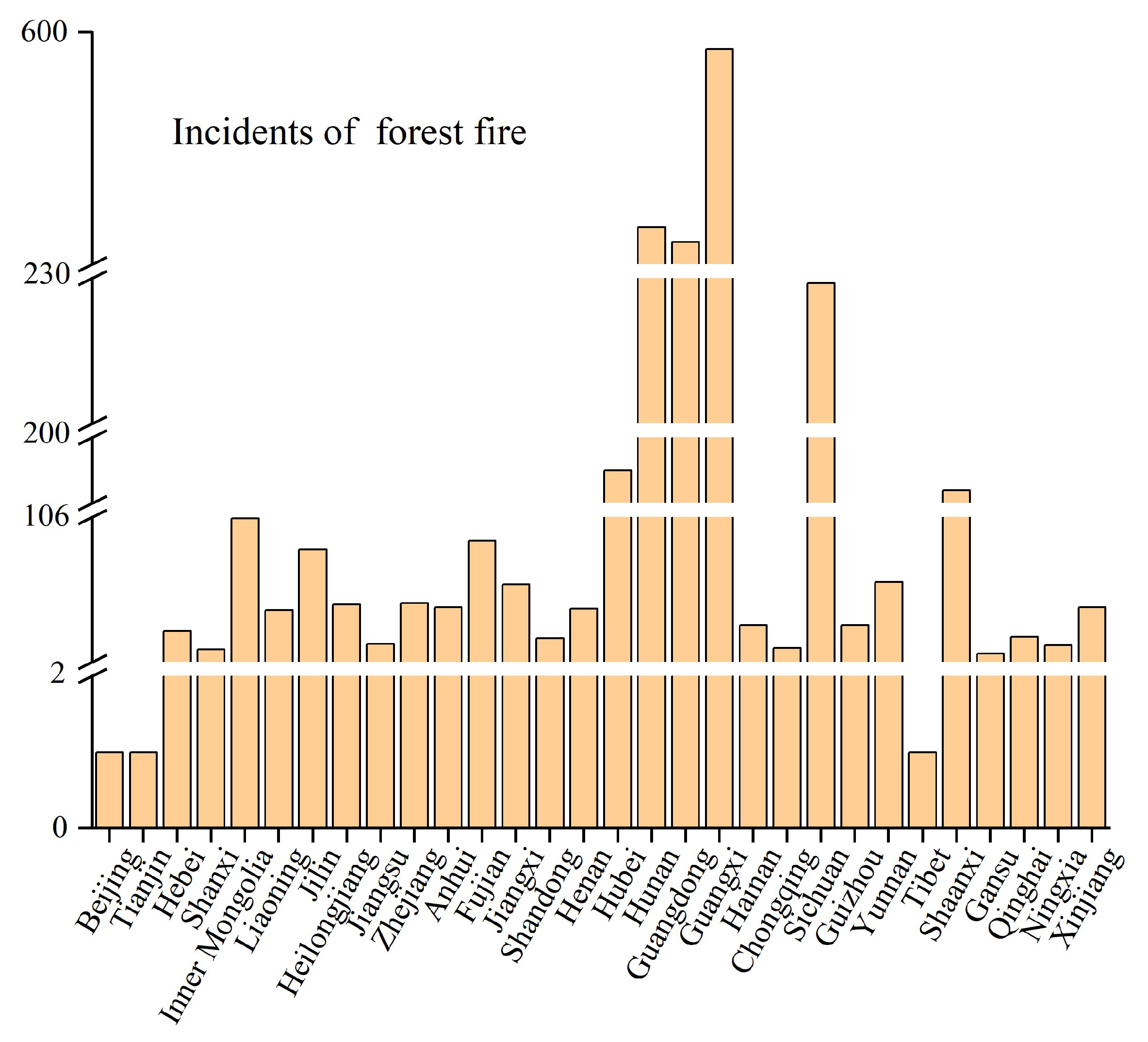
Figure 2.
Operational flowchart of the KOA-CNN-GRU-MHA model.
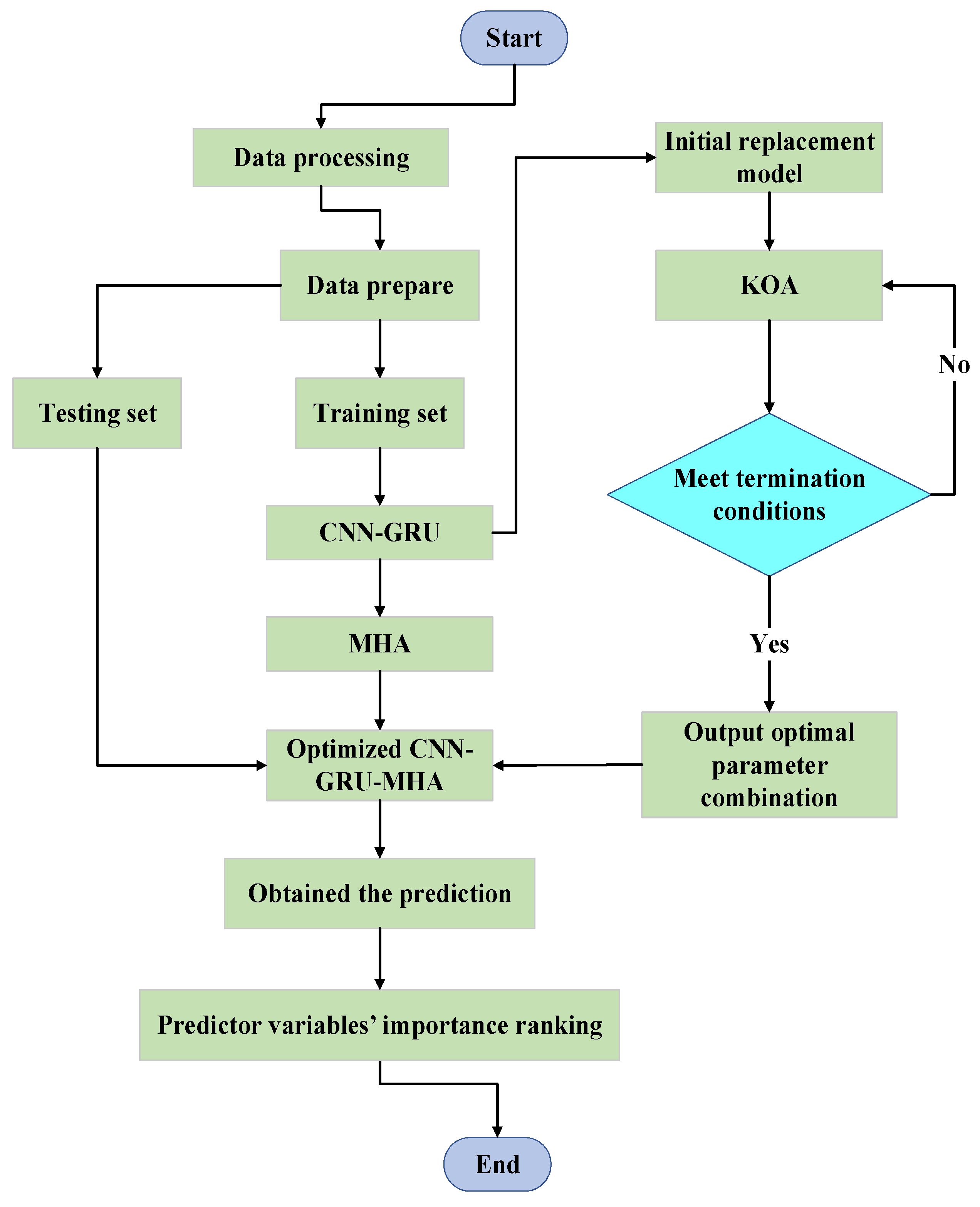
Figure 3.
Normality test histogram of the proposed variables.
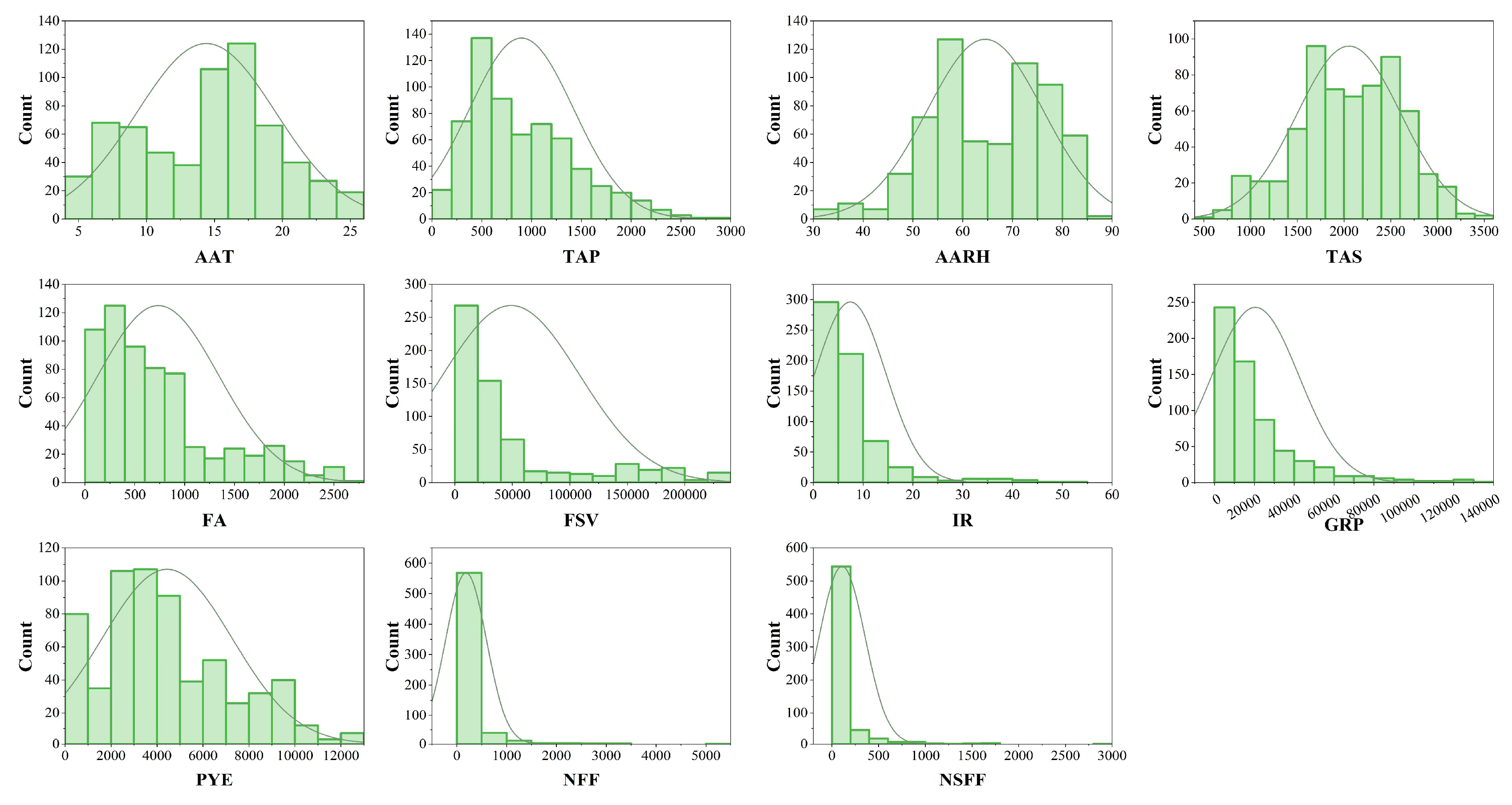
Figure 4.
Pearson correlation matrix between the predictor variables and the target variables.
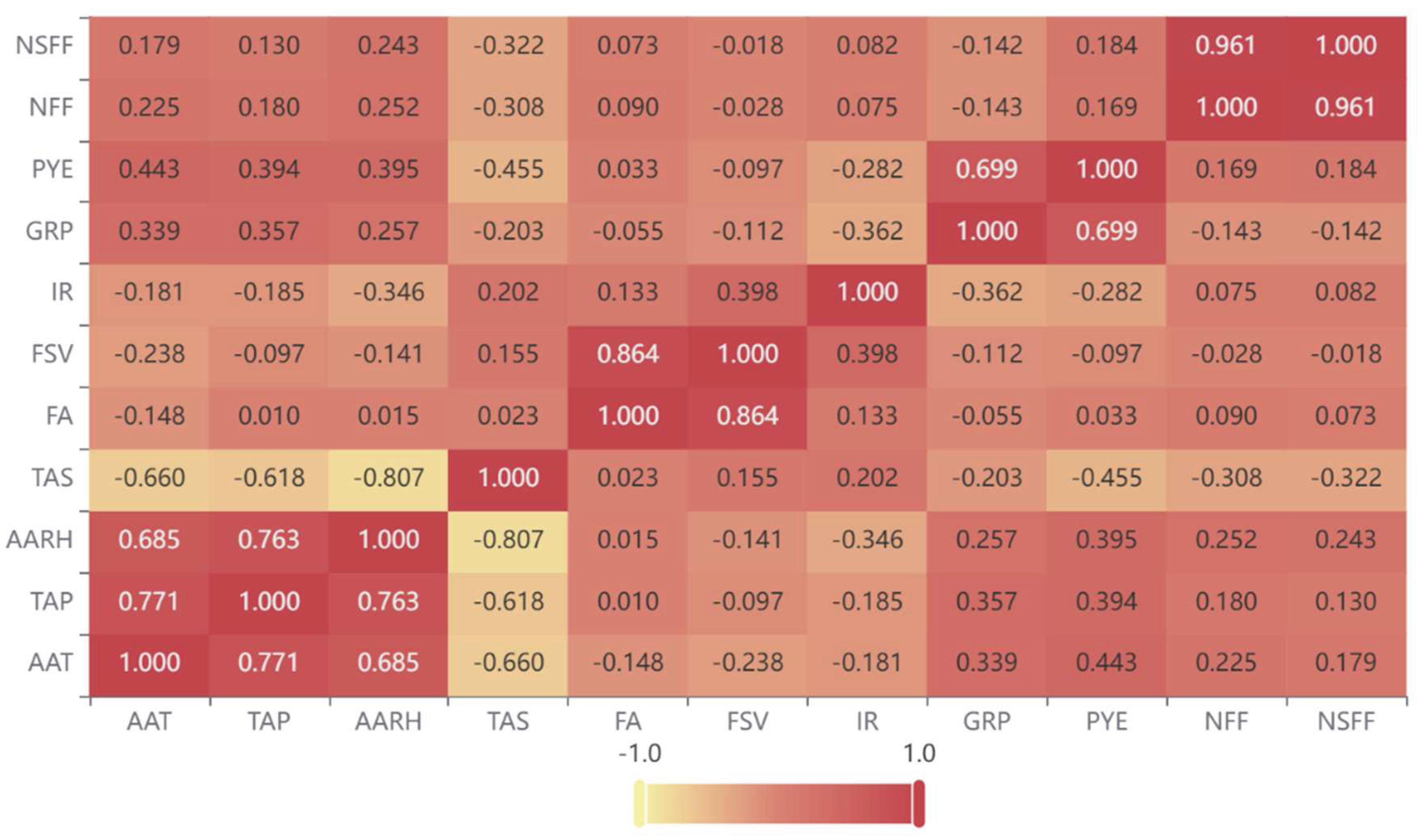
Figure 5.
NFF prediction errors for 30 Chinese provinces.
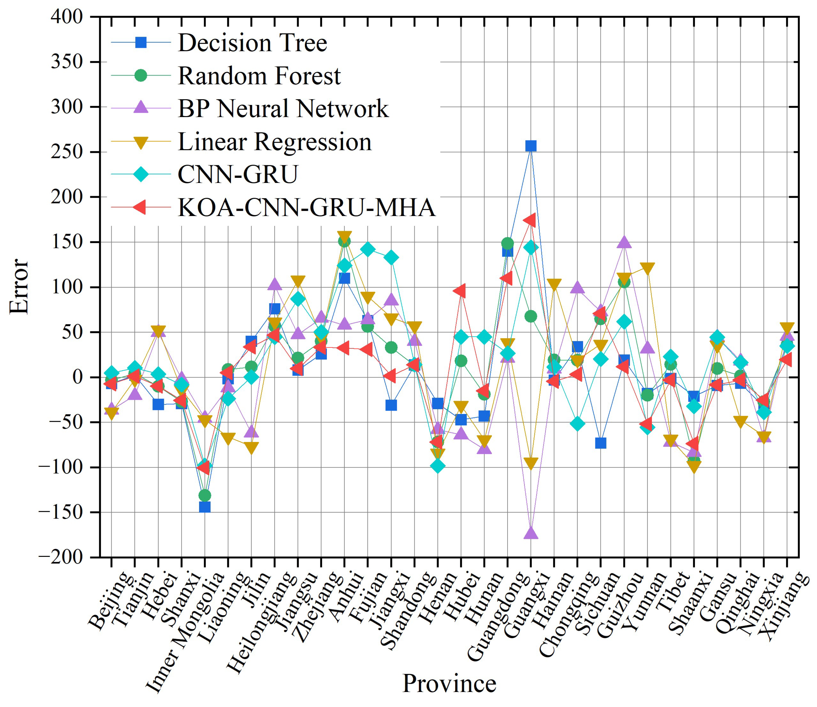
Figure 6.
NFF prediction results radar.
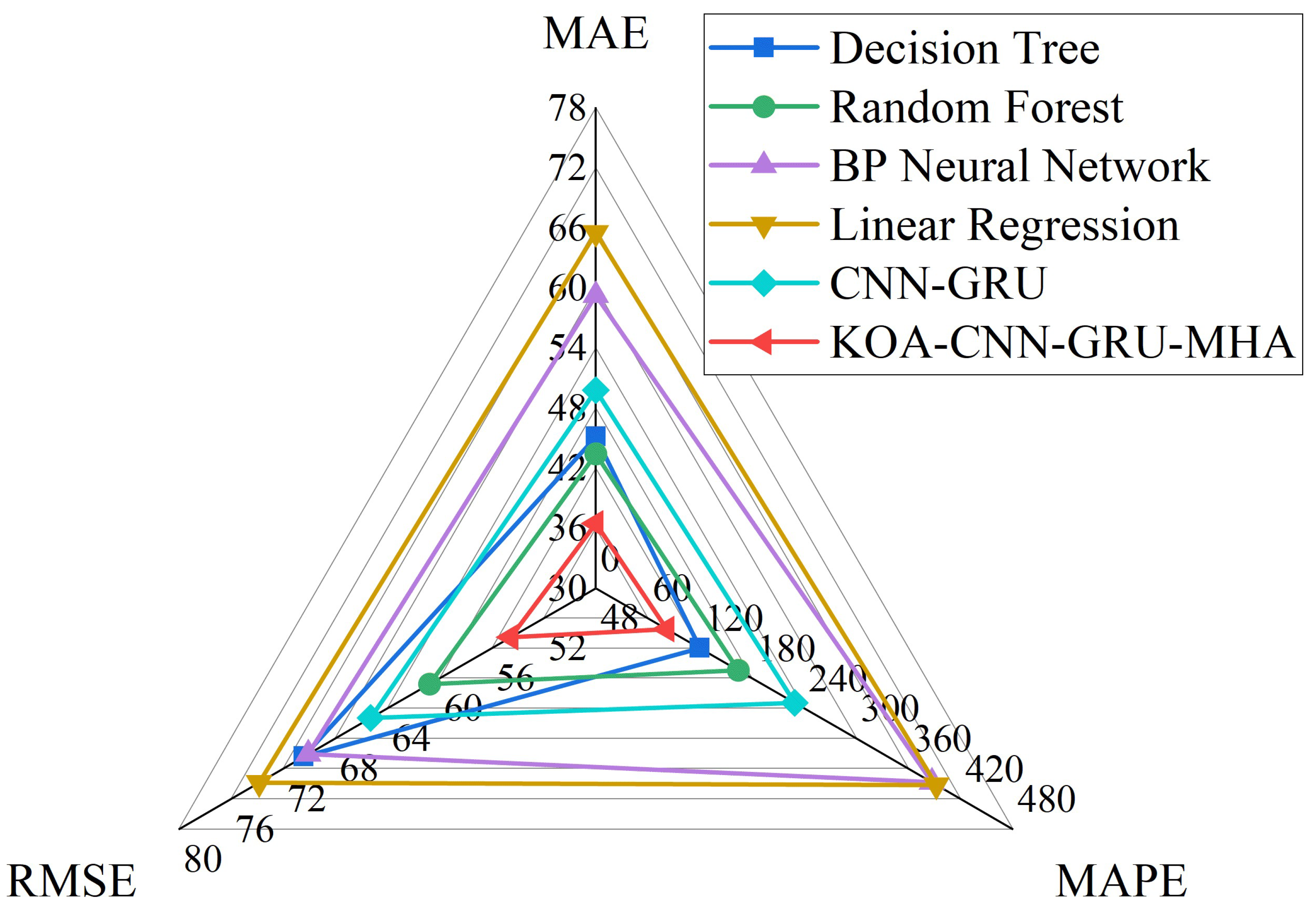
Figure 7.
Contribution of each variable to the NFF prediction results.
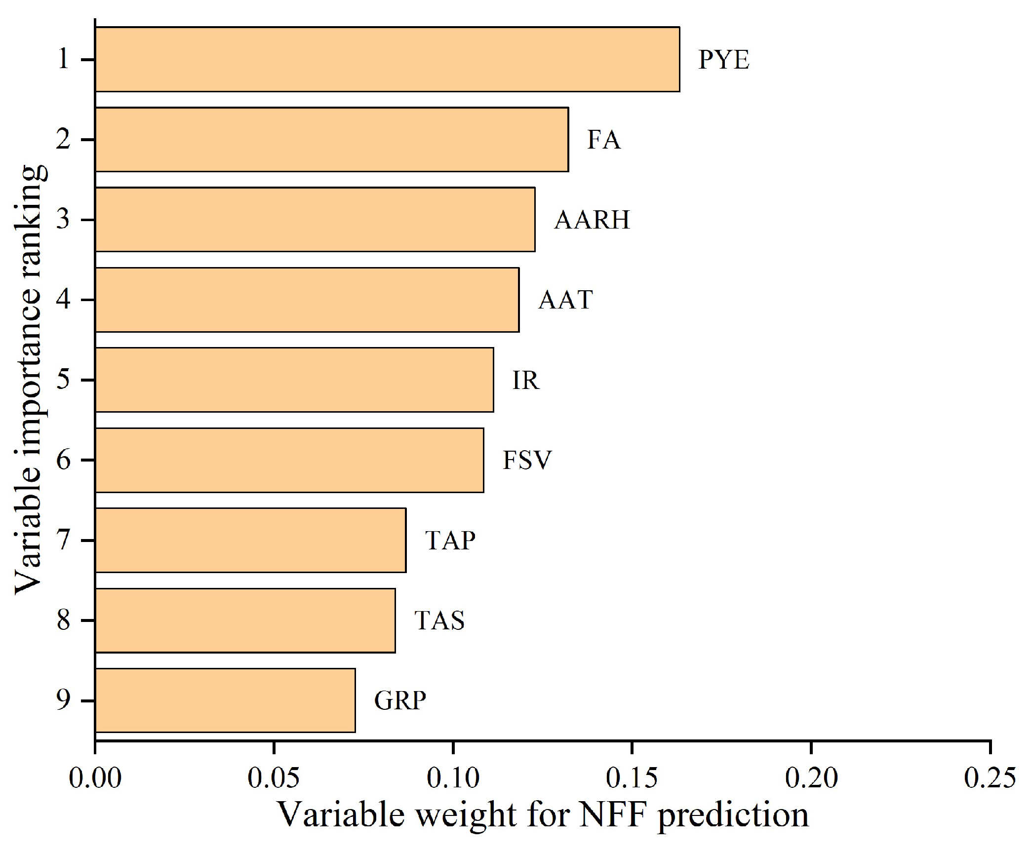
Figure 8.
NSFF prediction errors for 30 Chinese provinces.
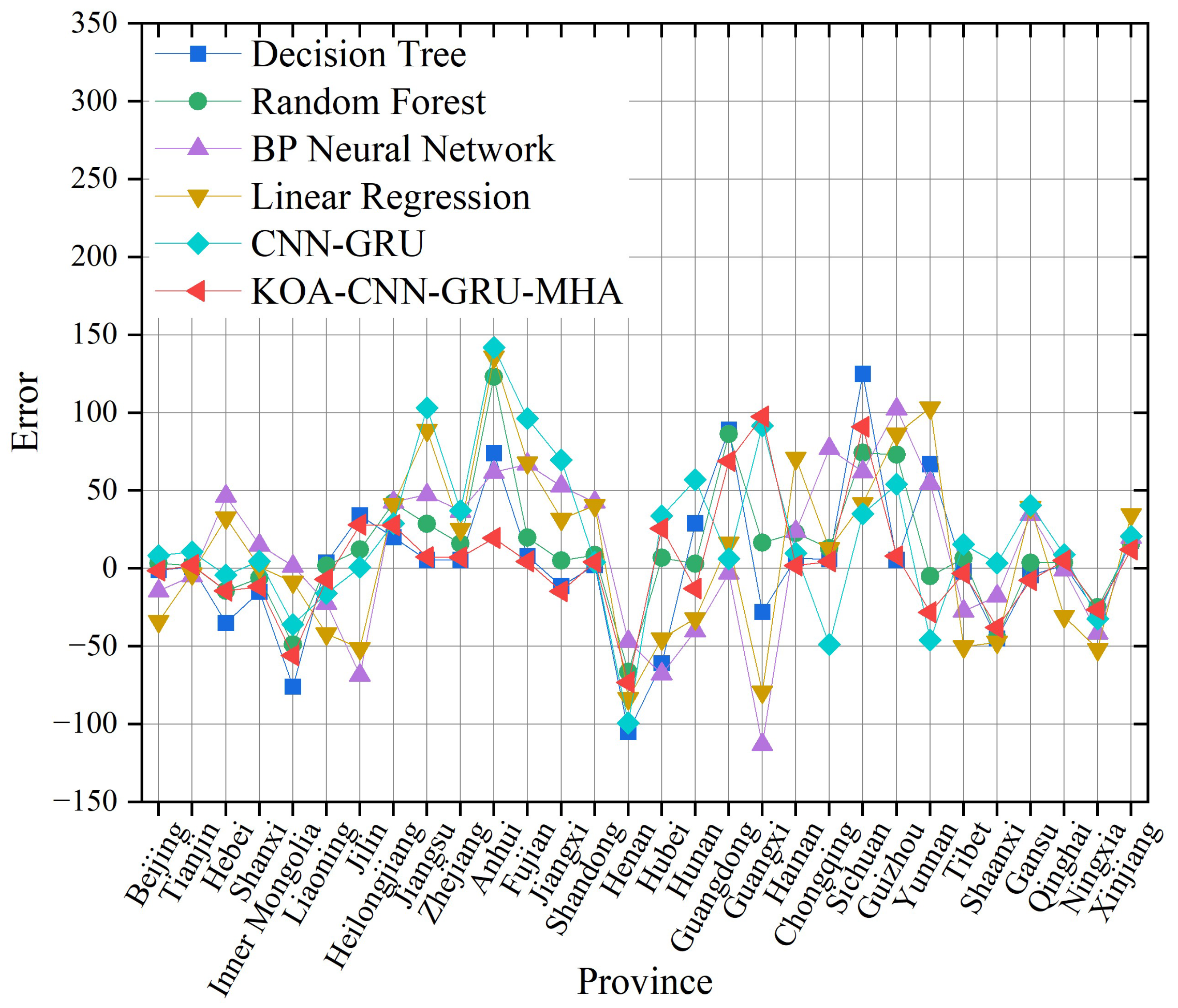
Figure 9.
NSFF prediction radar results.
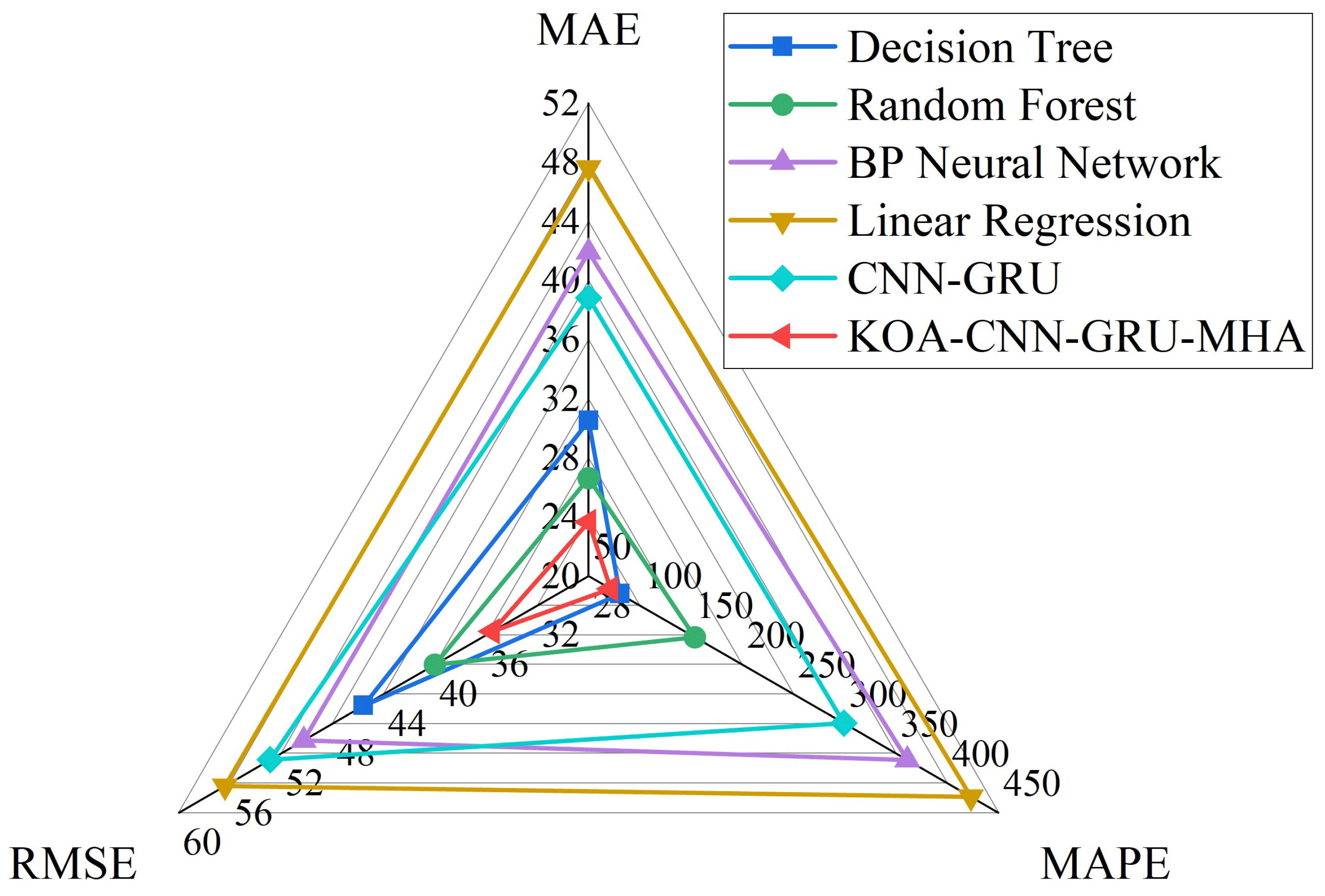
Figure 10.
Contribution of each variable to NSFF prediction results.
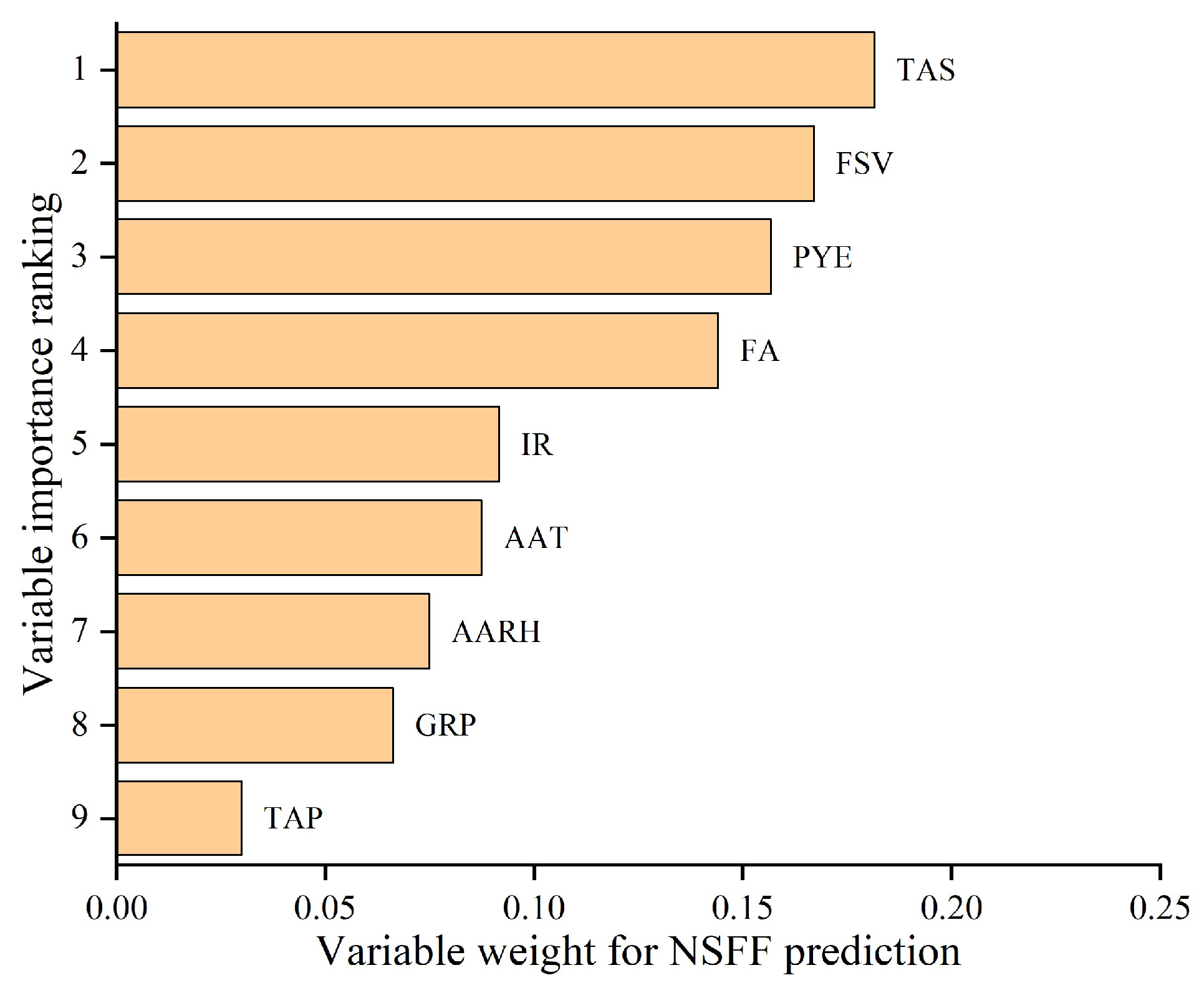

Table 1.
Summary of the predictor variables used in this study.
| Variable type | Abbreviation | Description | Prior Research |
| Climate condition | AAT | Annual average temperature | [51,52,53,54] |
| TAP | Total annual precipitation | [51,52,54] | |
| AARH | Annual average relative humidity | [1,51,55] | |
| TAS | Total annual sunshine | [10,25,51] | |
| Forest resource situation | FA | Forest area | [9,54,56] |
| FSV | Forest stock volume | [51,57,58] | |
| Socio–economic aspects | IR | The illiteracy rate among adults aged 15 years and older | [56,59,60,61] |
| GRP | Gross regional product | [10,51,62] | |
| PYE | Population at year-end | [10,61,63] | |
| Forest fire incidents | NFF | Total annual number of forest fires (the target variable) | [53,54,64] |
| NSFF | Total annual number of small forest fires that burnt less than one hectare (the target variable) | [65,66,67] |
Table 2.
Examples of partial forest fire data samples.
| Variable | Example values | |||||
| AAT (Celsius) | 12.8 | 12.7 | 13.6 | 10.1 | 7.1 | … |
| TAP (millimeter) | 444.5 | 668 | 641.1 | 525.4 | 653.1 | … |
| AARH (percent)) | 54 | 64 | 63 | 62 | 55 | … |
| TAS (hours) | 2260 | 1994 | 1724 | 2135 | 2474 | … |
| FA (ten thousand hectares) | 37.05 | 9.2 | 330.29 | 203.27 | 1935.51 | … |
| FSV (ten thousand cubic meters) | 809.72 | 144.33 | 6397.57 | 6088.74 | 107755.2 | … |
| IR (percent) | 4.61 | 6.36 | 7.35 | 5.79 | 13.67 | … |
| GRP (hundred million yuan) | 3663.1 | 2447.66 | 7098.56 | 2456.59 | 2150.42 | … |
| PYE (ten thousand persons) | 1456 | 1011 | 6769 | 3314 | 2386 | … |
| NFF (count) | 4 | 2 | 19 | 5 | 151 | … |
| NSFF (count) | 4 | 2 | 19 | 3 | 105 | … |
Table 3.
Performance of various models for NFF prediction.
| MAE | MAPE | RMSE | R² | |
| Decision Tree | 45.12 | 119.80 | 70.41 | 0.69 |
| Random Forest | 43.43 | 164.01 | 60.76 | 0.67 |
| BP Neural Network | 59.24 | 386.59 | 70.05 | 0.46 |
| Linear Regression | 65.52 | 391.88 | 73.82 | 0.46 |
| CNN-GRU | 49.79 | 228.84 | 65.27 | 0.70 |
| KOA-CNN-GRU-MHA | 36.47 | 81.59 | 54.52 | 0.80 |
Table 4.
Performance of various models for NSFF prediction.
| MAE | MAPE | RMSE | R² | |
| Decision Tree | 30.49 | 80.63 | 45.57 | 0.60 |
| Random Forest | 26.62 | 153.69 | 39.99 | 0.70 |
| BP Neural Network | 41.91 | 360.87 | 50.21 | 0.43 |
| Linear Regression | 47.63 | 422.69 | 56.37 | 0.37 |
| CNN-GRU | 38.83 | 298.92 | 52.84 | 0.65 |
| KOA-CNN-GRU-MHA | 23.66 | 71.64 | 35.50 | 0.82 |
Disclaimer/Publisher’s Note: The statements, opinions and data contained in all publications are solely those of the individual author(s) and contributor(s) and not of MDPI and/or the editor(s). MDPI and/or the editor(s) disclaim responsibility for any injury to people or property resulting from any ideas, methods, instructions or products referred to in the content. |
© 2026 by the authors. Licensee MDPI, Basel, Switzerland. This article is an open access article distributed under the terms and conditions of the Creative Commons Attribution (CC BY) license (http://creativecommons.org/licenses/by/4.0/).
Copyright: This open access article is published under a Creative Commons CC BY 4.0 license, which permit the free download, distribution, and reuse, provided that the author and preprint are cited in any reuse.