

Submitted:
21 July 2026
Posted:
21 July 2026
You are already at the latest version
Abstract
The response of premixed flames to external forcing is important for understanding flame dynamics and combustion instability. In this study, the velocity-field response of a laminar premixed propane–air flame under external forcing was investigated using particle image velocimetry, numerical simulation, and dynamic mode decomposition. The flame was studied under an unforced condition and several forced conditions at 20Hz and 80Hz, with an equivalence ratio of [0.95] and a Reynolds number of [800]. The results show that external forcing alters both the flame shape and the veloci-ty-field structure, and that the response is strongly frequency-dependent. The axial velocity component exhibits clear downstream convective propagation of the imposed disturbance, whereas the radial velocity response is mainly concentrated near the flame front and is associated with flame deformation and thermal expansion. Dynamic mode decomposition shows that the dominant coherent structures become weaker and decay more rapidly as the forcing frequency increases. The numerical results agree reasonably well with the experimental measurements for the unforced flame and pro-vide additional information on the downstream development of the forced flow. These results provide useful insight into forced flame-flow interaction in laminar premixed flames.
Keywords:
laminar premixed flame
; external forcing
; numerical simulation
; dynamic mode decomposition
; velocity response
1. Introduction
Premixed flames subjected to external perturbations exhibit complex dynamic responses arising from the coupling among flow unsteadiness, flame-surface deformation, heat release, and acoustic forcing. Such flame–flow interaction is closely related to the onset and development of combustion instability, which remains a major concern in practical premixed combustion systems, including gas turbines, industrial burners, and propulsion devices [1,2,3,4,5]. For this reason, understanding how an externally forced premixed flame responds in the velocity field and flame structure is of both fundamental and practical importance.
A large number of studies have shown that externally imposed disturbances can alter flame shape, propagation characteristics, and vortex–flame interaction patterns, thereby modifying the unsteady behavior of premixed flames [6,7,8,9,10]. Depending on the forcing frequency and amplitude, a premixed flame may undergo periodic wrinkling, large-scale oscillation, local curvature variation, and changes in convective transport [6,7,8,9]. These effects are especially evident in laminar premixed flames, which provide a well-controlled configuration for isolating the essential mechanisms of flame response under forcing [6,8,9]. Because of their relatively simple structure, laminar flames are often adopted as model systems for investigating the fundamental coupling between imposed flow perturbations and flame dynamics [7,8,9,10].
Among the available experimental approaches, particle image velocimetry (PIV) has been widely used to characterize the instantaneous and phase-dependent flow fields in reacting flows [11,12,13]. PIV makes it possible to quantify the axial and radial velocity components and thus provides direct evidence of how velocity disturbances propagate and interact with the flame front [11,12]. Previous studies based on optical diagnostics have shown that external forcing can induce periodic changes not only in the streamwise transport process but also in the transverse motion near the flame surface, where gas expansion and flame-front displacement become important [6,8,12].
However, experimental measurements are usually limited by the optical window, field of view, and spatial accessibility, especially in the downstream region of the flame. Numerical simulation can complement experiments by providing full-field information and by extending the analysis to regions that are difficult to access experimentally [14,15,16,17,18,19,20]. For premixed flames under periodic forcing, computational fluid dynamics (CFD) has been used to investigate the evolution of velocity perturbations, flame-surface deformation, and the interaction between unsteady flow structures and heat release [14,15,16,17,19,20,21]. When an appropriate combustion model is employed, numerical results can reproduce the main features of the measured flow field and help interpret the mechanisms underlying the experimentally observed response [14,15,16,17,18,19,20]. At the same time, comparison between simulation and experiment is valuable for assessing the predictive capability and limitations of the numerical framework [14,15,16].
To further extract coherent structures from time-resolved flow fields, dynamic mode decomposition (DMD) has become an effective analysis tool in combustion research [11,22,23,24,25,26,27]. Unlike conventional statistical methods, DMD directly identifies spatial modes associated with specific frequencies and growth or decay characteristics, making it particularly suitable for studying externally forced flames [22,23,24,25]. Recent studies have applied DMD to reacting flows to reveal dominant oscillatory structures, convective patterns, and mode-dependent flame responses under periodic excitation [11,23,24,25,26,27]. For velocity fields of premixed flames, DMD can distinguish between streamwise convective motion and transverse flame-coupled motion, thereby offering a more detailed physical interpretation of forced flame dynamics [11,22,23,26].
Despite these advances, comparatively less attention has been paid to the combined experimental and numerical characterization of both axial and radial velocity responses in laminar premixed flames under external forcing, especially with modal decomposition of the velocity field [11]. In particular, the distinct behaviors of axial and radial velocity components under different forcing frequencies have not yet been sufficiently clarified. Since the axial component is closely related to downstream transport of the imposed disturbance, whereas the radial component is more sensitive to flame-front movement and thermal expansion, a comparative analysis of the two components is necessary for a more complete understanding of flame response.
Therefore, the present study investigates the velocity-field characteristics of a laminar premixed propane–air flame under external forcing by combining PIV measurements, CFD simulations, and DMD analysis. The flame is examined under an unforced condition and forced conditions at 20 and 80 Hz, The operating conditions are fixed at an equivalence ratio of 0.95 and a Reynolds number of approximately 800. The objectives of this work are threefold: (1) to validate the numerical prediction of the unforced mean velocity field against PIV measurements; (2) to examine the frequency-dependent axial and radial velocity responses of the forced flame; and (3) to identify the dominant coherent structures in the velocity field using DMD and to interpret their physical significance. The results are expected to provide useful insight into the mechanism of externally forced flame–flow interaction and to support further studies of combustion instability in premixed systems.
2. Materials and Methods
2.1. Experiment Configuration and Operating Conditions
The experimental system used in the present study was based on our previous work [11] and consisted of a gas supply section, a plenum chamber, a burner, and a forcing device. Premixed propane and air were supplied to the burner through calibrated flow-control units and mixed upstream of the burner exit. A laminar premixed flame was stabilized at the burner outlet under atmospheric conditions. The burner had an outlet diameter of 9.5 mm, and the operating conditions were fixed at an equivalence ratio of 0.95 and a Reynolds number of approximately 800. The mean outlet velocity was 1.25 m/s.
To introduce periodic forcing, a loudspeaker mounted at the bottom of the plenum was used to impose harmonic excitation on the inlet flow. In the present work, the flame behavior under the unforced condition and under forcing frequencies of 20 and 80 Hz was analyzed in detail. The excitation altered the flow field upstream of the flame and induced periodic flame-front deformation [6,7,8,9].
Figure 1.
Schematic of the experimental setup and measurement system[11].
Figure 1.
Schematic of the experimental setup and measurement system[11].
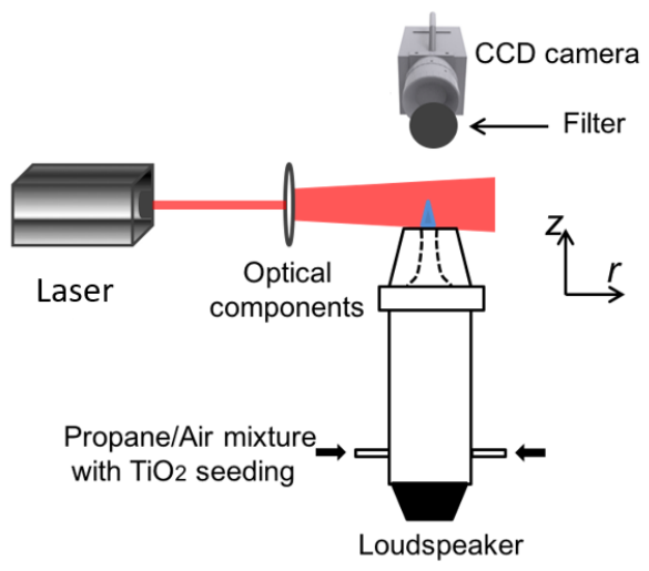
The global flame shape was recorded using optical imaging, and velocity measurements were performed by particle image velocimetry (PIV) [12,13]. Titanium dioxide (TiO₂) particles with a nominal diameter of approximately 1 μm were used as seeding particles. A dual-pulse laser system generated a laser sheet to illuminate the measurement plane, and the scattered light from the seeded particles was recorded by a CCD camera positioned normal to the laser sheet. The laser and camera were synchronized to acquire particle images for velocity-field reconstruction[11].
In the experiment, the high-speed camera has a resolution of 1030×800 pixels, a frame rate of 2000 fps, and a single-frame exposure time of 10 microseconds. In the PIV post-processing, PIVLAB software is used for data processing, with an interrogation window of 32×16 pixels for cross-correlation calculation, and the spatial overlap ratio between adjacent interrogation windows is 50%.
2.2. Numerical Setup
Numerical simulations were performed using ANSYS CFX [28,29] to reproduce the flow-field evolution of the forced premixed flame and to complement the PIV measurements. The computational domain was three-dimensional, with a cylindrical geometry of 100 mm in height and 200 mm in diameter. The mesh contained approximately 1.58 million tetrahedral cells.
Figure 2.
Computational domain and mesh.
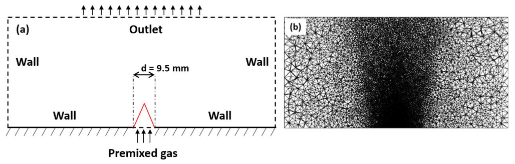
The governing equations were solved with the Reynolds-averaged Navier–Stokes framework [20,28]. Turbulence effects were modeled using the standard k–ε model. Combustion was treated using the Burning Velocity Model (BVM) available in ANSYS CFX [20,28]. For premixed combustion, the chemical kinetics can be represented by the mixture fraction and the species mass fractions[18,19,20].
where denotes the species diffusion coefficient.
By substituting the mass fraction with the reaction progress variable and the mixture fraction, Eq. (2) can be rewritten as.
The flow field can be divided into two distinct regions via introducing the reaction progress variable, which are the burned region and the unburned region. Unlike the continuous variation of the mass fractions of reactants and products in the flow field, the reaction progress variable is restricted to values of 0 (unburned) or 1 (burned) everywhere except in the vicinity of the flame front [18,19,20].
The reaction progress variable can be obtained by solving the species transport equation:
The propane/air premixed combustion flamelet library used in the calculations was generated using the RIF tool in CFX, and it consists of 35 species and 108 elementary reactions. The simulations were carried out under atmospheric pressure with the inlet mixture corresponding to an equivalence ratio of 0.95.
At the inlet, a harmonic velocity perturbation was imposed in the axial direction according to
whereis the mean inlet velocity, is the perturbation amplitude, and is the forcing frequency. The cases considered in the present study included the unforced condition and forced conditions at 20 and 80 Hz.
The time-dependent calculations were conducted for 10 forcing cycles for each forced case. The time step was set to 1 × 10⁻⁶ s.To facilitate modal analysis, the instantaneous velocity fields were stored at 50 snapshots per forcing cycle.
To identify the dominant coherent structures in the velocity field, dynamic mode decomposition (DMD) was applied to the time-resolved velocity snapshots obtained from both the PIV measurements and the numerical simulations [11,22,23,24,25,26,27]. DMD provides a decomposition of the flow field into spatial modes associated with specific temporal frequencies, and is therefore suitable for analyzing periodically forced flames [22,23,24,25].
In the present study, DMD was performed separately for the axial and radial velocity components. The purpose was to distinguish the dominant streamwise convective response from the transverse motion associated with flame-front deformation and gas expansion [11,22,23,26]. By comparing the DMD modes extracted from the experimental and numerical datasets, the consistency of the dominant forced response and the differences in modal amplitude and downstream development could be assessed [11,23,26].
The modal frequency corresponding to the inlet forcing was used as the principal basis for interpreting the results. Particular attention was paid to the spatial distribution of the dominant velocity modes, their downstream attenuation, and their relation to the flame-front location.

Table 1.
Summary of operating and forcing conditions.
| Case | Inlet_V(m/s) | Perturbation Amplitude(m/s) | Equivalence Ratio | Forcing Frequency(Hz) |
|---|---|---|---|---|
| Case_Unforced | 1.25 | 0.2625 | 0.95 | / |
| Case_20Hz | 1.25 | 0.2625 | 0.95 | 20 |
| Case_80Hz | 1.25 | 0.2625 | 0.95 | 80 |
3. Results and Discussion
3.1. Baseline Flame under the Unforced Condition
Before analyzing the forced cases, the velocity field of the unforced flame was examined to establish the baseline flow structure and to assess the performance of the numerical model. Figure 3 compares the mean axial velocity distributions obtained from the PIV measurements[11] and the numerical simulation under the unforced condition.
As shown in Figure 3, both PIV and CFD exhibit the same overall flow pattern: the axial velocity increases through the flame region and remains relatively high in the downstream burned-gas zone as a result of thermal expansion [18,19,20]. The simulation reproduces the main high-velocity region and the general spatial development of the mean flow field, indicating that the baseline flame structure is reasonably captured.
This agreement is further supported by the sectional velocity profiles in Figure 4. At all selected heights, the numerical results follow the measured radial variation of axial velocity well. With increasing axial distance, the profiles shift to higher velocity levels and show a more evident radial rise, reflecting the progressive acceleration of the flow induced by combustion[18,19,20]. The agreement in both trend and magnitude suggests that the numerical model captures the downstream development of the unforced flame with acceptable accuracy.
Small discrepancies can still be observed between the experimental and numerical profiles, especially in the slope of the radial increase and the exact location of the velocity rise at some axial positions. These differences are reasonable and may result from several factors, including uncertainties in PIV near regions of strong density gradient [12,13], slight mismatch in the flame-front position, and simplifications of the numerical model such as the turbulence and combustion treatment [14,18,20,28]. In addition, the experiment and simulation may differ in their sensitivity to local flame curvature and expansion effects, which can influence the detailed profile shape [7,18,20].
Overall, the consistency between the velocity contours and the sectional profiles demonstrates that the CFD model provides a reliable description of the mean flow field under the unforced condition. This validation supports its subsequent use for interpreting the forced flame response and the associated modal characteristics.
3.2. Axial Velocity Response under External Forcing
At 20 Hz, the axial velocity field exhibits a clear periodic evolution over one forcing cycle (Figure 5). Both the PIV measurements[11] and the CFX simulations show that the flame surface undergoes noticeable wrinkling and periodic displacement under the inlet forcing, while the overall flame still largely preserves its conical shape [6,7,8,9,10]. This suggests that the inlet disturbance is sufficient to induce a pronounced unsteady response, but not strong enough to destroy the large-scale flame topology.
In the unburned region, the axial velocity displays evident periodic fluctuations, indicating that the inlet disturbance is effectively convected toward the flame root and the upstream flame surface [8,9,10]. Meanwhile, in the burned region, the flow accelerates along both sides of the flame front and continues to develop downstream because of thermal expansion [7,18,19,20]. The phase evolution of this accelerated flow remains closely synchronized with the motion of the flame surface, implying that the axial response is governed not only by the incoming perturbation itself, but also by the flame-flow interaction induced by heat release and gas expansion [1,4,8,9,10].
In addition, a persistent low-velocity zone can be identified near the flame tip, and its position shifts upward and downward together with the oscillation of the tip. This feature indicates that momentum redistribution around the flame apex is also involved in the forced response. Therefore, under low-frequency forcing, the axial disturbance is not confined to the flame surface, but exhibits a relatively continuous propagation tendency into the downstream flow[8,9,10,11].
At 80 Hz, the axial velocity response becomes more localized around the flame, as shown in Figure 6. Under this higher forcing frequency, the flame front is more strongly wrinkled, and the original conical structure is no longer clearly maintained [6,8,10]. This indicates that faster inlet oscillations promote a more intense local deformation of the flame surface.
Although periodic axial velocity fluctuations are still observed in both the unburned and burned regions, confirming that the imposed disturbance continues to affect the entire reacting flow, the fluctuating structures become more compact and more concentrated near the flame. Meanwhile, the downstream continuity of the disturbance is weakened, and the streamwise propagation of the axial response becomes less pronounced[11,22,23,26].
This behavior suggests that, as the forcing frequency increases, a larger portion of the perturbation energy is consumed by local flame wrinkling and near-field flow adjustment, rather than being maintained in a coherent large-scale convective structure [8,10,26,30]. Therefore, compared with the 20 Hz case, the 80 Hz forcing enhances the local unsteady response of the flame, but reduces the ability of the axial disturbance to persist over a long downstream distance.
Figure 7 shows the DMD mode shape of the axial velocity field at 20 Hz. In the region covered by the PIV field of view, the experimental and numerical results agree well, especially in the distribution of the dominant modal structures around the flame surface and near the flame tip [11,22,23,26]. In both datasets, the largest modal amplitudes are mainly located along the two sides of the flame front and within the low-velocity region near the tip[11,22,26], indicating that the dominant axial mode is closely associated with flame-surface oscillation and downstream convective transport of the forced disturbance [11,22,23,26].
More importantly, the numerical result provides a more complete description of the downstream flow than the PIV measurement, whose field of view is restricted to the near-flame region. The CFX results clearly reveal that the disturbance generated near the flame does not remain confined to the reaction zone; instead, it is convected downstream with the burned gas and maintains a relatively large modal amplitude over a considerable axial distance. This feature highlights an important advantage of the numerical approach, namely, its ability to capture the full spatial development of the forced mode and to identify downstream propagation characteristics that cannot be fully resolved experimentally.
Although the modal amplitude predicted by the simulation is somewhat smaller than that measured by PIV, which may be attributed to numerical dissipation and the smoothing of small-scale unsteady structures, the numerical result still reproduces the main modal topology well. Therefore, the DMD analysis further supports the conclusion that the 20 Hz forcing gives rise to a coherent convectively dominated axial mode with clear downstream extension.
Moreover, Figure 8 presents the corresponding DMD mode shape at 80 Hz. Compared with the 20 Hz mode, the modal amplitude is significantly reduced, and the high-amplitude region becomes more tightly confined to the vicinity of the flame and the near-inlet flow. In the unburned region, the mode still retains a predominantly convective character, indicating that the incoming velocity fluctuation is first transported by the mean flow before interacting with the flame.
However, once the disturbance propagates downstream, its amplitude decays much more rapidly than in the 20 Hz case. This faster attenuation indicates that the high-frequency axial fluctuation is more strongly damped during transport and is less capable of maintaining a coherent large-scale structure in the downstream flow.
Therefore, the DMD result further confirms the trend observed in the phase-resolved velocity fields: the 80 Hz forcing mainly promotes a localized response near the flame, whereas its contribution to downstream axial propagation is comparatively limited.
3.3. Radial Velocity Response under External Forcing
Figure 9 presents the radial velocity mode shapes at 20 Hz obtained from the PIV measurements and the CFX calculations. In general, the fluctuation level of the radial velocity remains relatively low in the unburned region, indicating that the inlet forcing does not produce a strong transverse response before interacting with the flame. This feature is clearly different from the axial component, which can preserve a more evident convective signature in the upstream flow. For the radial component, the dominant response is instead concentrated near the flame front, suggesting that it is mainly induced by flame deformation and local flow adjustment rather than by direct streamwise transport of the inlet disturbance.
From the experimental result, it can be observed that the radial velocity fluctuation in the burned region also develops downstream in a convective manner. However, unlike the axial velocity mode, the radial component is only pronounced in the vicinity of the flame surface, while its magnitude remains comparatively weak in the unburned region and near the flame tip. This distribution indicates that the radial motion is closely associated with the wrinkling and lateral displacement of the flame front. In other words, once the incoming perturbation reaches the flame, part of the response is redistributed from the axial direction into the radial direction through flame-surface deformation and thermal-expansion-induced flow turning. As a result, the radial mode does not appear as a globally extended structure, but rather as a localized response attached to both sides of the flame.
The numerical result further reveals that the radial velocity component continues to develop along both sides of the flame surface and gradually forms a distinct antisymmetric velocity pattern in the downstream region. This antisymmetric structure reflects the out-of-phase lateral motion on the two sides of the conical flame, which is consistent with the alternating wrinkling of the flame sheet under periodic forcing. Compared with the PIV result, the CFX prediction provides a clearer view of the full downstream development of this structure, making it easier to identify how the near-flame radial fluctuation evolves into a paired antisymmetric mode farther downstream. This also suggests that, although the radial velocity amplitude is smaller than that of the axial component, it still carries important information on the transverse redistribution of momentum and on the coupling between flame wrinkling and flow response.
The radial velocity mode shape at 80 Hz is shown in Figure 10. Similar to the axial velocity mode, the amplitude of the radial component at 80 Hz is lower than that at 20 Hz. The fluctuating structure is still mainly confined to the vicinity of the flame, but its overall intensity is significantly weakened. This indicates that under higher-frequency forcing, the radial response becomes less effective in maintaining a coherent modal structure, even though the flame front itself may still undergo noticeable local deformation.
Another important feature is that the antisymmetric velocity region observed downstream at 20 Hz gradually weakens and eventually disappears at 80 Hz. This trend suggests that the downstream development of the radial mode is highly sensitive to forcing frequency. At the lower frequency, the perturbation has more opportunity to interact with the flame over a spatial scale comparable to the flame size, allowing the transverse motion on the two sides of the flame to organize into a recognizable antisymmetric pattern. By contrast, when the forcing frequency increases to 80 Hz, the corresponding disturbance wavelength becomes shorter, and the radial fluctuation decays more rapidly during downstream transport. As a result, the near-flame transverse response cannot be sustained over a long enough distance to form a clear large-scale antisymmetric structure.
For a conical flame whose characteristic size is much smaller than the disturbance wavelength, the radial velocity component is usually neglected because of its relatively small magnitude. However, the present results indicate that this simplification is not always appropriate. When the disturbance wavelength becomes comparable to the flame scale and the reaction zone undergoes obvious wrinkling, the role of the radial velocity component should not be ignored. Even if its absolute amplitude remains lower than that of the axial component, it directly reflects flame-surface displacement, lateral momentum redistribution, and the development of antisymmetric flow structures associated with flame deformation. Therefore, the radial mode provides a useful complementary perspective for understanding the dynamic response of the flame to inlet forcing, especially in cases where geometric-scale matching between the disturbance and the flame enhances transverse flow effects.
4. Conclusions
This study investigated the response of a laminar conical flame to acoustically induced velocity disturbances by combining PIV measurements and numerical simulations. The axial and radial velocity fields under different forcing frequencies were analyzed, and DMD was applied to extract the dominant velocity modes and clarify the flame–flow interaction. The main conclusions are as follows.
1. The flame response is strongly dependent on forcing frequency. Under the same inlet velocity amplitude, the flame surface exhibits different deformation characteristics at different frequencies. Lower-frequency forcing favors a more coherent global response, whereas higher-frequency forcing mainly enhances local flame wrinkling.
2. PIV measurements successfully captured the propagation characteristics of the forced flow field. Both axial and radial velocity disturbances exhibit convective modal features, but the axial component shows a more evident downstream propagation behavior.
3. The velocity-field evolution is closely coupled with flame motion. The radial velocity component remains weak in the unburned region, but becomes more significant near the flame surface and in the burned region due to flame wrinkling and thermal expansion.
4. The numerical approach reproduces the main structural features of the laminar flame and provides a wider view of downstream modal development. Although the predicted velocity amplitudes are slightly lower than the experimental results because of numerical dissipation, the simulations capture the essential flame–flow interaction characteristics well.
Author Contributions
Conceptualization, Ye Zhixian. and Hu Keqi.; methodology, Ye Zhixian.; software, Hu keqi.; validation, Xie Lan.; formal analysis, Xie Lan.; investigation, Xie Lan.; writing—original draft preparation, Hu Keqi.; writing—review and editing, Ye Zhixian.; visualization, Xie Lan. All authors have read and agreed to the published version of the manuscript.
Acknowledgments
The authors have reviewed and edited the output and take full responsibility for the content of this publication.
Conflicts of Interest
The authors declare no conflicts of interest.
References
- Candel, S. Combustion dynamics and control: Progress and challenges. Proc. Combust. Inst. 2002, 29, 1–28. [Google Scholar] [CrossRef]
- Keller, J.O.; Daily, J.W. Characterization of acoustic oscillations in combustion systems. J. Sound. Vib. 1998, 211, 657–675. [Google Scholar]
- Balachandran, R.; Ayoola, B.O.; Kaminski, C.F.; Dowling, A.P.; Mastorakos, E. Experimental investigation of the nonlinear response of turbulent premixed flames to imposed inlet velocity oscillations. Combust. Flame 2005, 143, 37–55. [Google Scholar] [CrossRef]
- Lieuwen, T. Modeling premixed combustion–acoustic wave interactions: A review. J. Propul. Power 2003, 19, 765–781. [Google Scholar] [CrossRef]
- Dowling, A.P. Nonlinear self-excited oscillations of a ducted flame. J. Fluid Mech. 1997, 346, 271–290. [Google Scholar] [CrossRef]
- Schuller, T.; Durox, D.; Candel, S. Dynamics of and noise generated by premixed flames. Combust. Sci. Technol. 2002, 174, 21–37. [Google Scholar]
- Law, C.K. Combustion Physics; Cambridge University Press: Cambridge, UK, 2006. [Google Scholar]
- Searby, G.; Clavin, P. Weakly nonlinear analysis of acoustically forced flames. Combust. Sci. Technol. 1986, 46, 167–190. [Google Scholar] [CrossRef]
- Noiray, N.; Durox, D.; Schuller, T.; Candel, S. A unified framework for nonlinear combustion instability analysis based on the flame describing function. J. Fluid Mech. 2008, 615, 139–167. [Google Scholar] [CrossRef]
- Palies, P.; Schuller, T.; Durox, D.; Candel, S. The combined dynamics of swirler and turbulent premixed swirling flames. Combust. Flame 2010, 157, 1698–1717. [Google Scholar] [CrossRef]
- Yang, Y.; Fang, Y.; Zhong, L.; et al. DMD analysis for velocity fields of a laminar premixed flame with external acoustic excitation. Exp. Therm. Fluid Sci. 2021, 123, 110318. [Google Scholar] [CrossRef]
- Boxx, I.; Stöhr, M.; Carter, C.D.; Meier, W. Temporally resolved planar measurements of transient phenomena in a partially premixed swirl flame in a gas turbine model combustor. Combust. Flame 2010, 157, 1510–1525. [Google Scholar] [CrossRef]
- Fansler, T.D.; Parrish, S.E. Spray measurement technology: A review. Meas. Sci. Technol. 2015, 26, 012002. [Google Scholar]
- Poinsot, T.; Veynante, D. Theoretical and Numerical Combustion, 3rd ed.; CERFACS: Toulouse, France, 2012. [Google Scholar]
- Moureau, V.; Domingo, P.; Vervisch, L. Design of a massively parallel CFD code for complex geometries. Comptes Rendus Mécanique 2011, 339, 141–148. [Google Scholar]
- Tay-Wo-Chong, L.; Bomberg, S.; Ulhaq, A.; Komarek, T.; Polifke, W. Comparative validation study on identification of premixed flame transfer functions. Combust. Flame 2012, 159, 1208–1218. [Google Scholar]
- Selle, L.; Schuller, T.; Ducruix, S.; Durox, D.; Candel, S. Modeling of the flame transfer function of a laminar premixed flame. Combust. Flame 2004, 137, 489–505. [Google Scholar]
- Zimont, V.L. Gas premixed combustion at high turbulence. Turbulent flame closure combustion model. Exp. Therm. Fluid Sci. 2000, 21, 179–186. [Google Scholar] [CrossRef]
- Peters, N. Turbulent Combustion; Cambridge University Press: Cambridge, UK, 2000. [Google Scholar]
- Veynante, D.; Vervisch, L. Turbulent combustion modeling. Prog. Energy Combust. Sci. 2002, 28, 193–266. [Google Scholar] [CrossRef]
- Illingworth, S.J.; Juniper, M.P. Nonlinear dynamics of thermoacoustic systems. Annu. Rev. Fluid Mech. 2020, 52, 1–29. [Google Scholar]
- Schmid, P.J. Dynamic mode decomposition of numerical and experimental data. J. Fluid Mech. 2010, 656, 5–28. [Google Scholar] [CrossRef]
- Rowley, C.W.; Mezic, I.; Bagheri, S.; Schlatter, P.; Henningson, D.S. Spectral analysis of nonlinear flows. J. Fluid Mech. 2009, 641, 115–127. [Google Scholar] [CrossRef]
- Chen, K.K.; Tu, J.H.; Rowley, C.W. Variants of dynamic mode decomposition: Boundary condition, Koopman, and Fourier analyses. J. Nonlinear Sci. 2012, 22, 887–915. [Google Scholar] [CrossRef]
- Tu, J.H.; Rowley, C.W.; Luchtenburg, D.M.; Brunton, S.L.; Kutz, J.N. On dynamic mode decomposition: Theory and applications. J. Comput. Dyn. 2014, 1, 391–421. [Google Scholar] [CrossRef]
- Hemati, M.S.; Rowley, C.W.; Deem, E.A.; Cattafesta, L.N. De-biasing the dynamic mode decomposition for applied Koopman spectral analysis. Theor. Comput. Fluid Dyn. 2017, 31, 349–368. [Google Scholar] [CrossRef]
- Kaiser, E.; Noack, B.R.; Cordier, L.; Spohn, A.; Segond, M.; Abel, M.; Daviller, G.; Östh, J.; Krajnović, S.; Niven, R.K. Cluster-based reduced-order modelling of a mixing layer. J. Fluid Mech. 2014, 754, 365–414. [Google Scholar] [CrossRef]
- ANSYS Inc. ANSYS CFX-Solver Theory Guide, Release 2020 R2; ANSYS Inc.: Canonsburg, PA, USA, 2020. [Google Scholar]
- ANSYS Inc. ANSYS CFX Reference Guide, Release 2020 R2; ANSYS Inc.: Canonsburg, PA, USA, 2020. [Google Scholar]
- Lieuwen, T.; Yang, V. Combustion Instabilities in Gas Turbine Engines: Operational Experience, Fundamental Mechanisms, and Modeling; AIAA: Reston, VA, USA, 2005. [Google Scholar]
Figure 3.
Comparison of the mean axial velocity field between PIV and numerical simulation under the unforced condition.
Figure 3.
Comparison of the mean axial velocity field between PIV and numerical simulation under the unforced condition.
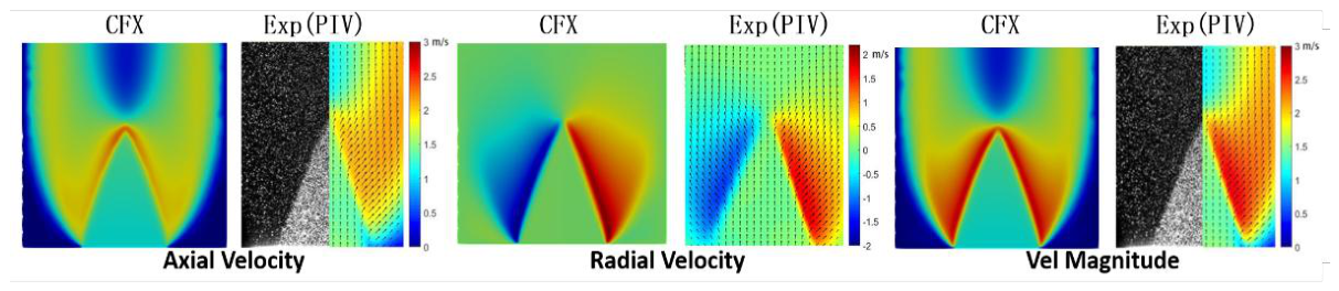
Figure 4.
Comparison of radial profiles of axial velocity between experiment and numerical simulation at different axial locations under the unforced condition.
Figure 4.
Comparison of radial profiles of axial velocity between experiment and numerical simulation at different axial locations under the unforced condition.
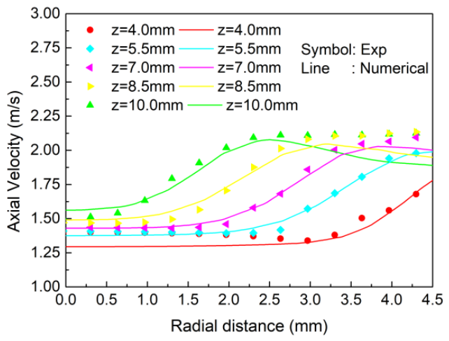
Figure 5.
Axial velocity perturbation field under 20 Hz.
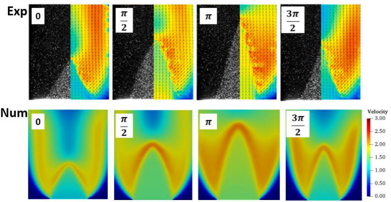
Figure 6.
Axial velocity perturbation field under 80 Hz.
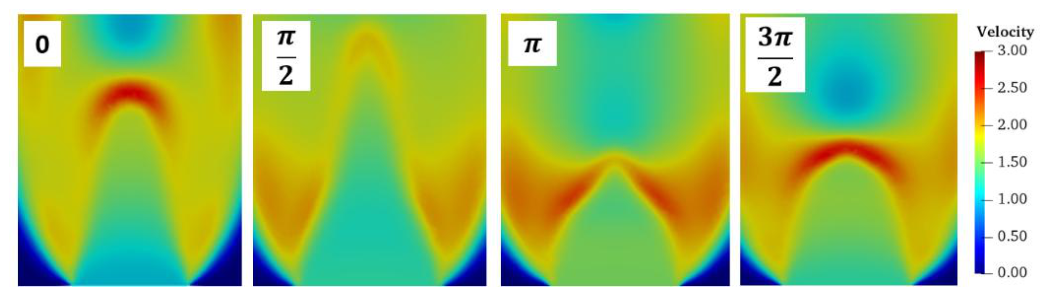
Figure 7.
Axial velocity modal contours at 20Hz from Experiment[11] and CFD.
Figure 7.
Axial velocity modal contours at 20Hz from Experiment[11] and CFD.
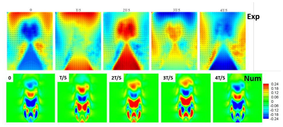
Figure 8.
Axial velocity modal contours at 80 Hz (from CFD).
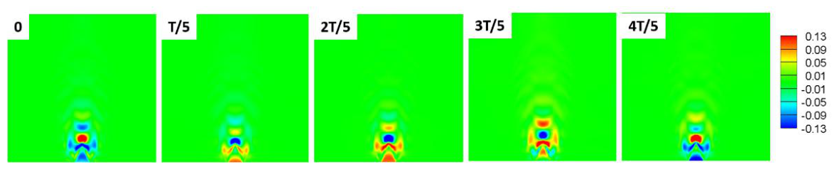
Figure 9.
Radial velocity modal contours at 20Hz from PIV[11] and CFD.
Figure 9.
Radial velocity modal contours at 20Hz from PIV[11] and CFD.
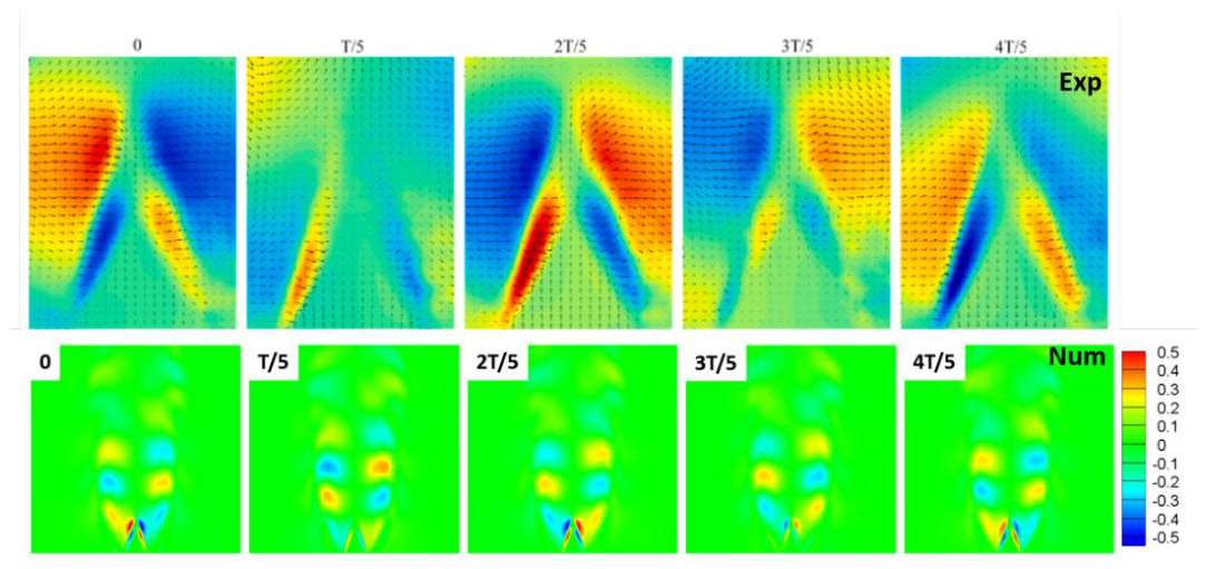
Figure 10.
Radial velocity modal contours at 80Hz(from CFD).
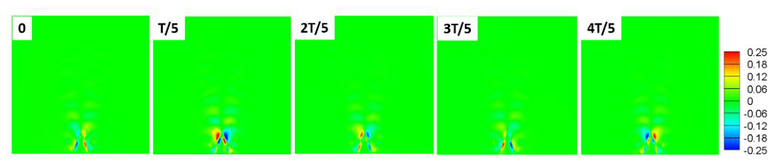
Disclaimer/Publisher’s Note: The statements, opinions and data contained in all publications are solely those of the individual author(s) and contributor(s) and not of MDPI and/or the editor(s). MDPI and/or the editor(s) disclaim responsibility for any injury to people or property resulting from any ideas, methods, instructions or products referred to in the content. |
© 2026 by the authors. Licensee MDPI, Basel, Switzerland. This article is an open access article distributed under the terms and conditions of the Creative Commons Attribution (CC BY) license (http://creativecommons.org/licenses/by/4.0/).
Copyright: This open access article is published under a Creative Commons CC BY 4.0 license, which permit the free download, distribution, and reuse, provided that the author and preprint are cited in any reuse.


