
Submitted:
17 July 2026
Posted:
20 July 2026
You are already at the latest version
Abstract
This work presents the first complete system for automated six degrees of freedom (6DOF) satellite pose estimation from spatially resolved, ground-based, adaptive optics (AO)-corrected imagery, addressing a key challenge in Space Domain Awareness (SDA). The approach eliminates the need for human labeling by directly regressing satellite orientation and position from blurry, noisy, and deeply-shadowed imagery. A multi-stage deep neural network pipeline localizes the satellite, predicts pose, and optionally applies temporal smoothing. Networks are trained exclusively on fully synthetic imagery generated from a CAD model, yet generalize effectively to real data, bridging the Sim2Real domain gap. On 137 real, human-labeled test images of Seasat, the model achieved a mean rotation error of 5 degrees and a mean image-plane translation error of 21 cm. Qualitative evaluation of additional real Seasat imagery rated 178 of 199 predicted poses as “ground truth equivalent” or “high confidence match,” with zero catastrophic failures. The system was extended to seven degrees of freedom (7DOF) for satellites with articulating components and demonstrated on real Hubble Space Telescope (HST) imagery, achieving 5.9 degrees rotation error, 48 cm translation error, and 6 symmetry-adjusted solar array error on a 249-frame pass with temporal filtering. Across 586 real test images from Seasat and HST (captured over multiple decades under diverse conditions) the system consistently performed well. On a high-fidelity wave optics (HFWO) synthetic test set of Seasat, the model achieved 8.4 degrees mean rotation error, 34 cm image-plane translation error, and 1.4% range error at r0=6 cm and 1,031 km range. It outperformed human labeling in both accuracy (48% lower rotation error) and speed (800× faster at 7.1 Hz inference), while requiring < 40 hours on a single A100 GPU to train. The approach was also demonstrated for ARGOS, a smaller satellite with highly symmetric geometry. A GIQE-based image quality metric was introduced to forecast pose accuracy. General-purpose models like GPT-4o and Depth Anything V2 failed across most SDA tasks, but rapid gains in vision-language models warrant continued monitoring. These results establish a new operational baseline for practical, real-time satellite pose estimation from AO SDA imagery.
Keywords:
satellite pose estimation
; adaptive optics
; space domain awareness
; sim2real
; domain gap
; deep learning
; 6DOF
; n-DOF
1. Introduction
Automated satellite pose estimation has the potential to enhance spacecraft health assessment, pattern-of-life analysis, and space traffic management, becoming an integral component of future Space Domain Awareness (SDA) architectures. Large-aperture, ground-based Electro-Optical (EO) instruments routinely collect adaptive optics (AO)-corrected, spatially resolved imagery of low Earth orbit (LEO) satellites [1]. In practice, difficulties arising from visual ambiguity and labor intensive workflows mean that few of these images are used for pose estimation. Automating pose estimation from such imagery would enable timely characterization of satellite behavior, thereby increasing the operational value of mission-relevant AO assets. Additionally, the rapidly growing population of objects in LEO motivates increased automation.
This work addresses monocular 6dofsix degrees of freedom (6DOF) pose estimation, the recovery of both three degrees of freedom (3DOF) position and 3DOF orientation from a single image. 6DOF pose is illustrated in Figure 1a, and 6DOF pose estimation is illustrated in Figure 1b. In some cases, like the articulating solar arrays on the Hubble Space Telescope (HST) that track the Sun with one rotational DOF, estimating additional DOF is required. The problem is tractable for SDA because the data already exists but the exploitation remains technically challenging under realistic conditions: partial illumination with deep shadows, variable and often low signal-to-noise ratio, poor contrast, residual blur which varies with atmospheric conditions and AO-system performance, and significant variation in target slant range. While this image quality challenge (illustrated in Figure 2) can be overcome with supervised learning and large datasets, there is limited labeled real data available for this application. Therefore models must be trained entirely in simulation, and any Sim2Real domain gap between synthetic training data and real imagery must be overcome.
Two precursors explored satellite pose estimation from such imagery. Wood [3] introduced a matched filter-based approach that demonstrated classification of discrete two degrees of freedom (2DOF) rotations using synthetic imagery with full front illumination and fixed image-plane translation and target range, an important starting point that did not address full 6DOF pose and lacked validation on real data. Lucas et al. [4] presented the first end-to-end deep learned approach, predicting 3DOF rotation using quaternion regression on synthetic AO imagery, showing promising results on pristine renders, but degraded accuracy with realistic residual AO blur (uncorrected atmospheric distortion). Image-plane translation and target range were fixed and not estimated, the renders were fully front illuminated, and no real imagery was tested . These studies established the problem, highlighted core challenges, and demonstrated key techniques and advancements but did not deliver a practical capability suitable for operational SDA.
Progress in direct pose regression has been driven by two main developments that inform this work. First, GDR-Net [5] and its predecessor CDPN [6] showed that semantic-segmentation-guided supervision with dense pixelwise 2D↔3D correspondences and a learned pnp-inspired regression head can effectively replace classical pnp/Random Sample Consensus (RANSAC). This approach elegantly simplifies the learning of the continuous output-space pose regression task by way of a semantic segmentation geometric classification task, which has a discrete output space that has arguably better learnable mappings and reduced loss surface complexity. These works also introduced and employed Scale-Invariant Representation for Translation Estimation (SITE), which is adopted and adapted for this work. Subsequent variants of GDR-Net, including GDR-NPP [7] and GPose2023 [8], improved robustness and won the 6D Object Localization tasks of the Benchmark Object Pose (BOP) 2022 and 2023 challenges [9,10]. Second, the continuous 6D representation for 3DOF rotation (Ref. [11], employed in GDR-Net and subsequent variants) eliminates discontinuities present in other 3DOF representations (like quaternions) and stabilizes training for direct pose regression. The representation allows incorporation of Gram-Schmidt orthogonalization as a layer within the regression head, enforcing learning and output of physically valid 3DOF rotations (orthonormal rotation matrices, special orthogonal group in 3D ()). This representation paired with in-network orthogonalization is now standard in leading pose regression models and is adopted here.
Lessons from the Satellite Pose Estimation Challenge (SPEC) further shape the approach. Satellite Pose Estimation Challenge 2019 (SPEC2019) [12] established the strength of sparse keypoint correspondences and pnp/RANSAC pipelines on synthetic Rendezvous and Proximity Operations (RPO) imagery, while Satellite Pose Estimation Challenge 2021 (SPEC2021) [13] emphasized bridging the Sim2Real domain gap using challenging and highly realistic Hardware-In-the-Loop (HIL) test images and simple synthetically rendered training images. Park et al. (2023) introduced SPNv2 with multi-task learning, the 6D rotation representation, and domain-specific randomized augmentations that target realistic illumination, blur, and noise distributions. They later added temporal processing and improved efficiency for edge deployment [14,15,16]. Their approaches for randomized augmentation and processing strongly inspired this work. Although SPEC was limited to 6DOF, did not provide a cadCAD model, and used high resolution space-based RPO imagery rather than lower quality ground-based AO imagery, the challenge and resulting publications provided a wealth of knowledge to inform the model architecture, data generation, and augmentation choices employed here.
The purpose of this study was to develop and validate a practical system that estimates full ≥6DOF pose from resolved, monocular, grayscale AO imagery in real time and trained using only synthetic data. The approach uses a three-stage pipeline: a custom Coarse Localizer to detect the satellite and crop down to the Region of Interest (RoI), a direct regression PoseNet inspired by GDR-Net [5], and an adaptive Kalman filter for temporal smoothing. Training used renders produced from 3D CAD models and domain-specific randomized image augmentations that simulate blur, noise, and illumination variation representative of real AO imagery. Rotation regression uses the 6D representation [11] and augmentations were informed by SPEC and Park et al. (2023) [13,14]. The result is a direct regression model trained solely on synthetic AO-like imagery with the ability to generalize to real AO data with accuracy sufficient to enable pose estimation workflow automation. This work assumes a single instance of a single object in the field of view and a CAD model available at train-time.
Our main contribution is a practical ≥6DOF system that operates in real time (>7 Hz) and, despite being trained solely on synthetic imagery, was demonstrated to successfully generalize to 586 real images of two separate satellites (Seasat and HST) captured by two distinct AO systems from two independent ground sites (located in New Mexico and Hawaii) over more than a decade. The approach was demonstrated to exceed human pose labeling in accuracy and speed. The work further quantifies how pose accuracy relates to atmospheric /AO-system performance, image quality, and illumination conditions. This work evaluates a modern Vision-Language Model (VLM) on SDA imagery, finding it currently inadequate for this task. The methods described and evaluated here advance beyond prior efforts [3,4], leverage BOP-era direct-regression [5,10] and the 6D rotation representation [11], incorporate SPEC-inspired Sim2Real insights [12,13,14], and establish a new baseline for automated LEO satellite pose estimation from ground-based, AO-corrected imagery. Uniquely, this approach is capable of enhancing real-time sensor operator situational awareness, as shown in Figure 3. Preliminary results were published in the proceedings of the 2024 AMOS Conference [17], and additional methodological detail and complete results are available in [18].
2. Materials and Methods
2.1. Approach Overview
Large-scale synthetic data are generated with Blender/EEVEE using site-specific terminator illumination, scaled orthographic rendering, and AO-point spread function (PSF) inspired degradations based on an empirical 2D double-Gaussian PSF [19]. A learned end-to-end pipeline performs coarse amodal localization followed by 6DOF pose regression (extendable to n-DOF by applying main body pose-aware branched regression heads). Optionally, temporal filtering is applied when time-series data are available. Besides the grayscale image, two application-specific inputs are injected throughout: an illumination direction unit 3-vector in image coordinates and an orthographic scale estimate (object-plane horizontal field of view (HFOV), a linearly scaled proxy for target range). Model architectures are shown in Figure 14 and Figure 16 and implemented entirely in TensorFlow [20]. High Fidelity Wave Optics (HFWO) closed-loop AO-corrected imagery was simulated for test-time evaluation (Section 2.4).
2.2. Imaging Geometry, Coordinates, and Camera Model
Topocentric azimuth and elevation for the Sun are computed with Astropy across a full year and restricted to morning/evening terminators (three hours before sunrise to sunrise, sunset to three hours after sunset) [21]. These coordinates are perturbed by additive noise sampled from a normal distribution, , to augment the dataset. Samples for which the Sun-target vector intersects the Earth were excluded using a spherical Earth model with a radius of , chosen to prevent erroneously discarding valid terminator geometries (Figure 4a). The range of Sun positions present during terminator conditions at a fixed site varies by <0.1° over 20 years, supporting trained model reuse across years but not across ground sites. Target azimuth angles were sampled uniformly (Figure 4b), while zenith angles were drawn from a uniform distribution U on with a power-law transformation with exponent 0.4, i.e., . This biases the resulting elevations, , toward lower values (Figure 7), with the constraint that target elevation angles exceed 30°.
Topocentric Sun and target distributions for training data are displayed in Figure 4. The render camera employs scaled orthographic projection at px. The Instantaneous Field of View (IFOV) is selected so that the target’s longest axis subtends ≤50% of the image HFOV at minimum range; for Seasat this yields nrad. Alternatively, the IFOV can be selected to equal that of a real system or to be a multiple of a real system’s IFOV. This was done for HST, where simulation IFOV nrad was selected as double the true system IFOV. Blender axes follow right, up, out of the image plane (sensor-to-target).
To stabilize optimization under megameter-scale Z and decimeter-scale , a SITE-style normalization is adopted from [5,6] and adapted for this work, using the slant range to calculate a target-plane HFOV in meters, normalize by the minimum HFOV, then divide by the RoI zoom ratio (Section 2.5.4). Coudé rotation is accounted for by (i) test-time derotation, (ii) uniform in-plane rotations applied to the training data illumination vectors, or (iii) telescope-specific analytic angles derived from az/el (preferable when the coudé path is known).
2.3. Synthetic Training Data Generation
With the imaging geometry established, this section details the pipeline used to generate the richly-annotated synthetic dataset. The process begins with an accurate 3D CAD model and systematically applies realistic, application-specific degradations designed to bridge the Sim2Real domain gap.
2.3.1. Scene Configuration
Seasat CAD imagery is rendered for unique 6DOF pose+illumination pairs at px (80%/10%/10% train/validation/test). For each pose, EEVEE produces a partially illuminated render and a paired fully front-illuminated render (for relighting supervision). Material properties were inspired by [22] with randomized per-sample perturbations to reflect uncertain real-world material properties.
2.3.2. Sampling of Pose, Illumination, and Range
Rotations are sampled uniformly on ([23]), yielding the expected quaternion element histograms after normalization (Figure 5). World translations are approximately uniform in angle-space with the constraint of maintaining the complete object within the field of view (FOV), as displayed in Figure 6. In practice, sensor operators “click-track” if necessary to ensure objects are fully within the FOV. Target elevation is constrained to ≥30° (image quality is significantly degraded <30° due to increased target range and atmospheric path length); target zenith angles (Figure 7) and Sun positions are as described previously.
Slant range d is approximated with the spherical Earth form [24]:
with elevation and satellite altitude h. In this specific application, the spherical Earth approximation results in slant range errors of less than 0.1%, which was deemed acceptable. Future work may incorporate a more accurate model such as WGS 84.
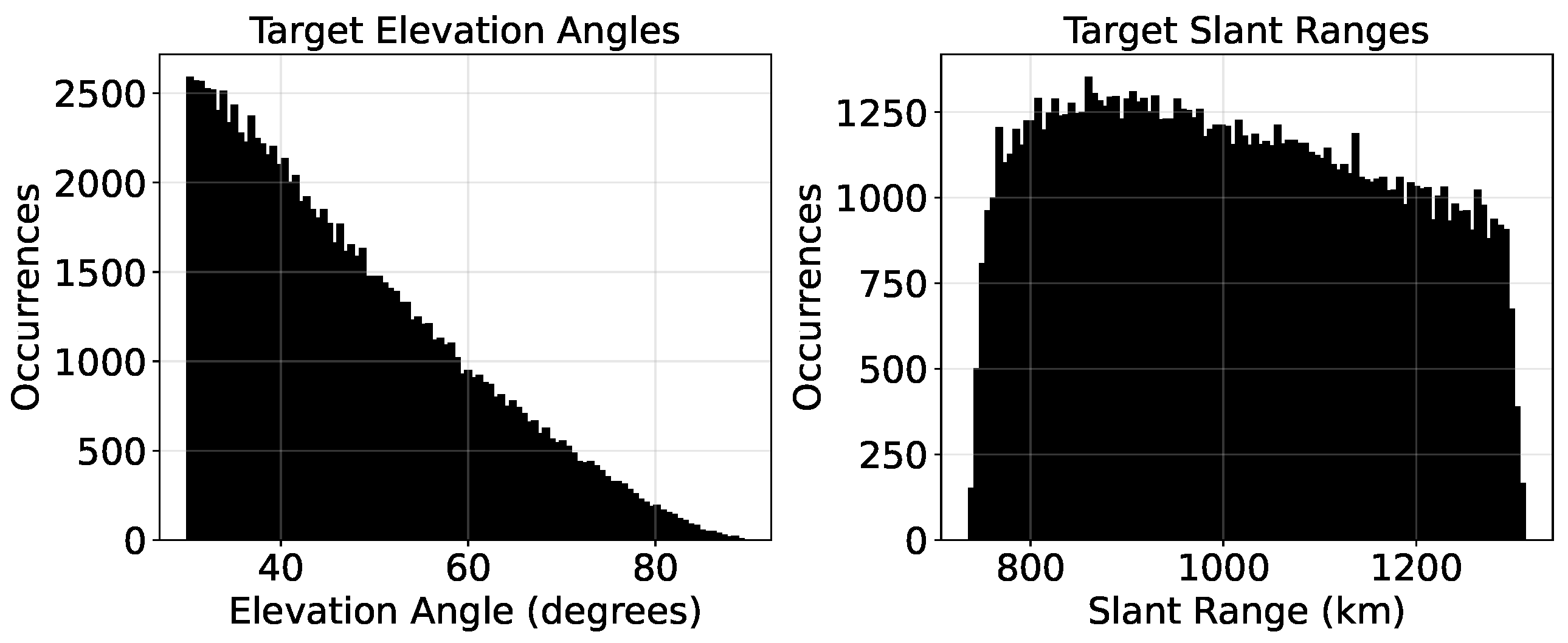
Figure 7.
Histograms of training set target object elevation angles (left) and camera-target slant ranges (right). The distribution of elevation angles was intentionally biased to produce a more uniform distribution of slant ranges.
Figure 7.
Histograms of training set target object elevation angles (left) and camera-target slant ranges (right). The distribution of elevation angles was intentionally biased to produce a more uniform distribution of slant ranges.
2.3.3. Rendered Supervision and Label Construction
For each sample the following are produced: RoI-cropped pristine image; RoI-cropped pristine front-lit image; dense per-pixel world coordinates; 33-class surface-region labels obtained via farthest-point sampling on the fused point cloud [5]; and maps that encode the full-frame coordinates of RoI pixels (Figure 8, Figure 9 and Figure 10). These labels drive the staged training of the PoseNet (Section 2.5.3). The number of regions was set to 32 (plus one background class) to balance accuracy and computational cost, a choice informed by the ablation study in [5] which demonstrated 70.5% accuracy versus 71.0% accuracy for 32 and 64 regions, respectively.
2.3.4. AO-Style Degradations and Augmentations
Inspired by [14], application-specific randomized augmentations are applied to the pristine renders to better simulate the appearance of real AO imagery. These augmentations are critical for bridging the Sim2Real domain gap, as underscored by SPEC2021 [13]. A 2D double-Gaussian PSF is used to approximate time-averaged AO blur. Ghost images are randomly synthesized by summing spatially shifted and scaled variants of the PSF to emulate high-frequency jitter. Random specular glints are also injected as isolated 2D Gaussian peaks positioned within the satellite bounding box, simulating transient solar reflections from satellite surfaces. A realistic sensor noise model combines four components: dark current, fixed pattern noise, Poisson-distributed shot noise, and Gaussian read noise. Additional noise augmentations include standalone Gaussian noise and multiplicative intensity noise (both pixelwise and image-wide). Brightness, contrast, gamma, and bias (pedestal) adjustments are also randomly applied. Other randomized degradations include additional motion blur, median blur, and Gaussian blur. Sensor artifacts such as hot pixels, dead pixels, and coarse dropout (random small rectangular occlusions) further increase realism and broaden the distribution of the training data (with the goal of encompassing the distribution of possible real imagery). Each transformation is applied randomly and independently with a tuned probability. The resulting training set includes images, derived from unique pose and illumination combinations. Low Fidelity In-Distribution (LFID) validation and test sets, each comprising unique samples, are degraded using the same augmentation pipeline. Neural style transfer [14,16,25,26] was considered for future use but omitted here due to the limited availability of real AO satellite imagery. While applying augmentations dynamically at batch draw time can be more robust, a fixed set of augmentations was pre-generated for this work to simplify prototyping and coupled training between the Coarse Localizer and PoseNet. The double-Gaussian blur, ghost images, specular glints, sensor noise model, bias, hot pixel, and dead pixel implementations were custom while the remaining augmentations used [27].
2.3.5. Randomized MLI Texture
2.4. Synthetic Test Data Generation
Due to the limited availability of labeled real imagery for model validation, high-fidelity synthetic test data were created using a fully independent process to create a simulated domain gap (Sim2Sim). Digital Imaging and Remote Sensing Image Generation (DIRSIG) was used to render object planes and High Contrast Imaging for Python (HCIPy) was used to generate realistic AO PSFs and realistic noise via a simulated closed-loop AO system using wave optics and random atmosphere with temporal coherence [28,29,30]. A notional AO system was simulated with specifications similar to [31,32]. The HCIPy simulation produced broadband PSFs with enhanced realism and complexity compared to the empirical Gaussian PSFs used for the training data. This pipeline controlled for atmospheric conditions such as the Fried parameter, [33,34], enabling quantification of relationships between pose model accuracy and atmospheric turbulence and image quality. Noteworthy enhancements for the DIRSIG renders are:
- Inclusion of Earth’s surface as an additional illumination source.
- Use of a physics-based MODTRAN atmosphere model.
- Lunar contributions to both direct object illumination and atmospheric path radiance.
- Support for multi-bounce surface reflections.
- Physics-based camera model with perspective projection.
- Extended Sun source (0.5°) producing soft shadow edges.
- Validated computation of 32-bit at-aperture radiance in W/cm2/sr/µm.
In contrast, the Blender simulation lacked Earth and lunar illumination sources, did not simulate atmospheric effects or path radiance, excluded multi-bounce reflections, used a simple scaled orthographic projection, treated the Sun as a point source, and output unitless 8-bit pixel values. A comparison of Seasat renders produced with Blender and DIRSIG is shown in Figure 12. While effective at synthesizing labeled, highly realistic SDA AO imagery for model validation the Blender+DIRSIG pipeline currently requires >10 s of computation per frame, making it impractical for synthesizing viably sized training sets. An HCIPy-simulated AO PSF is displayed in Figure 13. HFWO images are displayed in Figure 27, Figure 29, Figure 31, Figure 32.
2.5. Learning System
2.5.1. Coarse Localizer
The localizer (Figure 14) regresses amodal boxes and object center in continuous image coordinates: . Inputs are the grayscale image, a 3-channel illumination vector (constant across the grid, normalized to ), and an orthographic scale estimate similarly replicated across the full image-dimension grid to fill a channel. A U-Net backbone (M parameters) first predicts a reconstructed+relit image; two heads (M parameters each) then regress the box (Complete Intersection over Union (CIoU) loss) and center (Mean Squared Error (MSE) loss) [35,36]. Amodal supervision enables the RoI crop to center the CAD origin, reducing residual translation for PoseNet. A custom Coarse Localizer was used in contrast to [5] due to the unique properties of this imagery, the fact that Faster R-CNN [37] required additional training time, and to take advantage of additional application-specific inputs (target range, illumination direction).
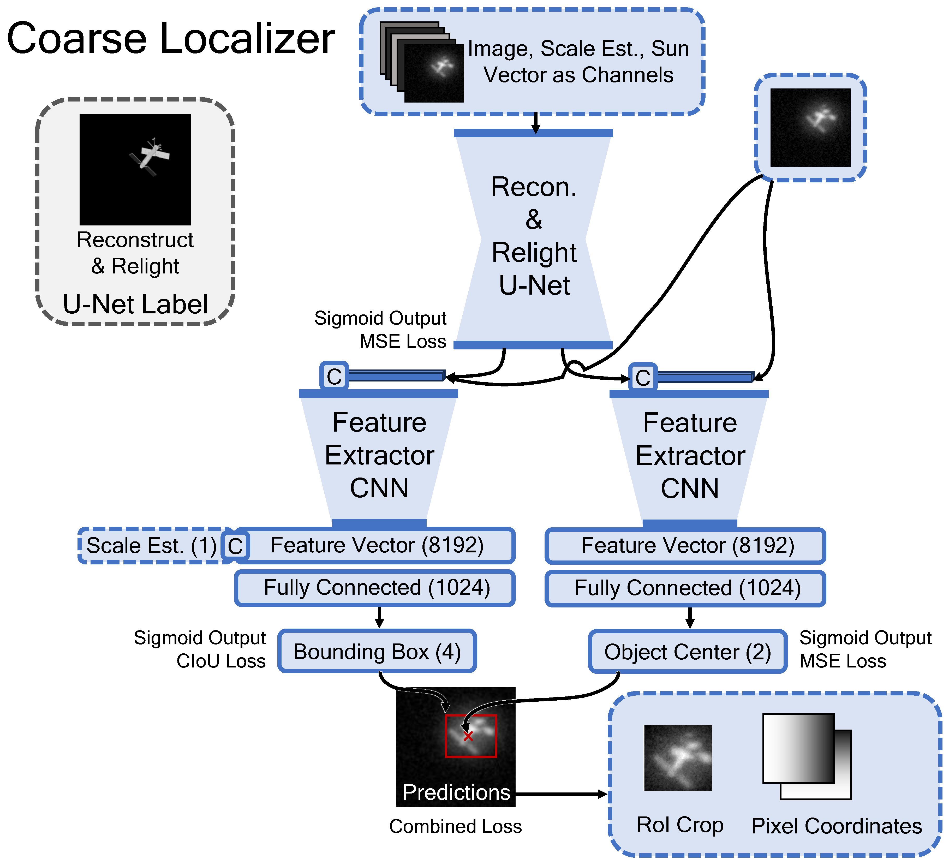
Figure 14.
Architecture of the Coarse Localizer. The Coarse Localizer takes in 256×256 pixel grayscale images, illumination vectors, and normalized orthographic scale estimates (object plane HFOV in meters). It first uses a U-Net backbone to regress an intermediate reconstructed and relit image which is then fed (along with the initial input image) into two separate convolutional neural network (CNN) heads to output bounding box coordinates and object center coordinates. These outputs are used to crop and resize the input image to a 64×64 pixel RoI and to generate pixel coordinate maps.
Figure 14.
Architecture of the Coarse Localizer. The Coarse Localizer takes in 256×256 pixel grayscale images, illumination vectors, and normalized orthographic scale estimates (object plane HFOV in meters). It first uses a U-Net backbone to regress an intermediate reconstructed and relit image which is then fed (along with the initial input image) into two separate convolutional neural network (CNN) heads to output bounding box coordinates and object center coordinates. These outputs are used to crop and resize the input image to a 64×64 pixel RoI and to generate pixel coordinate maps.
2.5.2. RoI Crop, Resize, and Maps
The RoI algorithm enforces: (1) square crop before resize; (2) RoI contains the full predicted amodal bounding box; (3) predicted center at RoI center. Zero-padding is applied if needed. The crop is resized to and paired with maps () that preserve each pixel’s location in the original frame, serving as dense 2D keypoints for 2D↔3D correspondences. Training is coupled: PoseNet consumes localizer predictions rather than randomly perturbed ground truth, matching test-time failure modes (Figure 15). This is done because of the broad distribution of image quality produced by AO instruments and the strong correlation between localizer performance and image quality. Coupled training preserves this correlation, though special care must be taken in training not to overfit the model to the training set.
2.5.3. PoseNet for 6DOF (extendable to n-DOF)
PoseNet (Figure 16) comprises four compact U-Nets (backbone) feeding a cnnCNN pose regressor head:
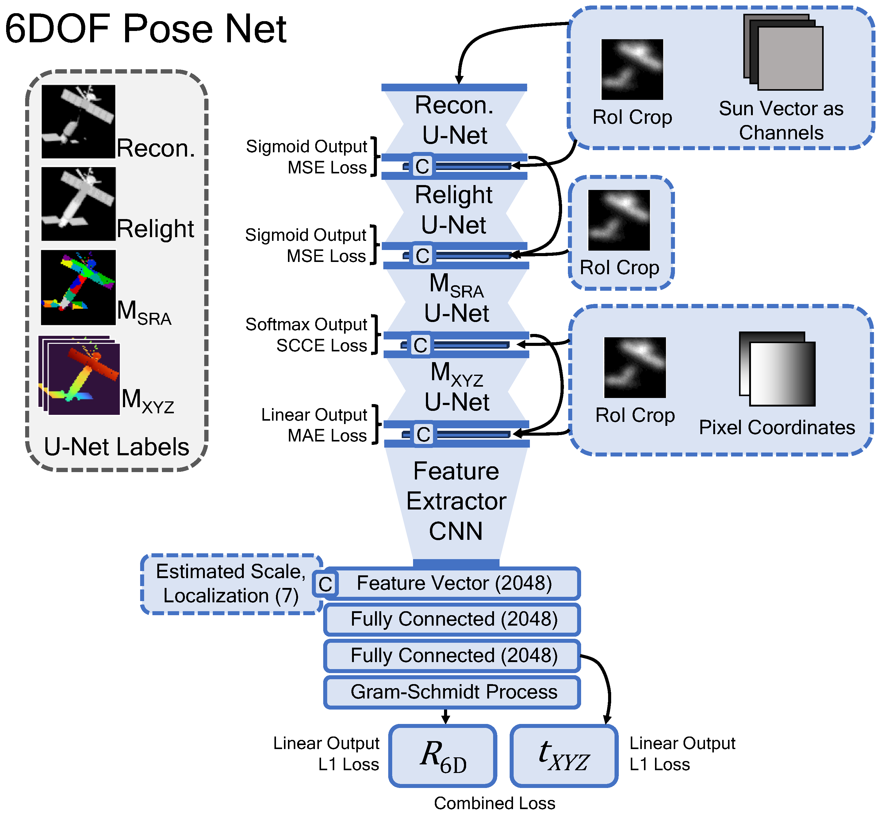
Figure 16.
Architecture diagram for the PoseNet. The PoseNet takes in the RoI image, the pixel coordinate maps, an orthographic scale estimate (a representation of target slant range that is calculated based on known camera intrinsic parameters and a two-line element set (TLE)), the predicted bounding box coordinates, and the predicted object center coordinates. The PoseNet predicts 6DOF pose, with surface region attention maps and 3D point maps being intermediate outputs.
Figure 16.
Architecture diagram for the PoseNet. The PoseNet takes in the RoI image, the pixel coordinate maps, an orthographic scale estimate (a representation of target slant range that is calculated based on known camera intrinsic parameters and a two-line element set (TLE)), the predicted bounding box coordinates, and the predicted object center coordinates. The PoseNet predicts 6DOF pose, with surface region attention maps and 3D point maps being intermediate outputs.
- 1.
- Reconstruction U-Net: inputs = RoI + 3-ch illum. vector; output = denoised/deblurred image.
- 2.
- Relighting U-Net: inputs = RoI + 3-ch illum. vector + denoised/deblurred image; output = fully front-lit (deshadowed) image.
- 3.
- U-Net (32 object surface region classes, 1 background class): inputs = RoI + reconstruction output + relighting output; output = class logits.
- 4.
- U-Net: inputs = + RoI + ; output = dense world (set-normalized to range ).
The regressor ingests a 41-channel tensor (concatenating RoI, reconstruction output, relighting output, , , ). A 7D auxiliary vector [scale, , is provided as input at the feature vector (first dense layer). Orientation uses the continuous 6D representation [11] followed by Gram-Schmidt orthogonalization to ; translation is linear. The full model has M parameters; further increasing parameters by adding nodes to the dense layers while holding the training set constant did not improve model accuracy.
2.5.4. Scale Normalization
2.5.5. Training Schedule and Losses
Optimization uses Adam [38] with the default initialized learning rate of unless otherwise stated and all training employs early stopping () on validation loss. Stage 1: train reconstruction+relighting U-Nets jointly with a combined loss; freeze. Stage 2: train ; freeze. Stage 3: train , briefly unfreeze upstream for end-to-end finetuning with learning rate initialized to ; refreeze. Stage 4: train the CNN pose regression head (Figure 17). Losses are: MSE (reconstruction/relighting), sparse categorical cross-entropy (), Mean Absolute Error (MAE) (). The final disentangled pose loss is
without weighting, as adopted from [5].
2.5.6. Articulations (n-DOF)
To incorporate a single rotational articulation, the disentangled pose loss in Section 2.5.5 is extended with a symmetry-aware term with the sine-cosine representation :
where and . The operator enforces 180° symmetry (antipodal equivalence) appropriate for highly symmetric solar-array geometry and stabilizes training. On pristine synthetic 7DOF Seasat imagery, the raw solar array articulation error is 90° (random guessing), whereas the symmetry-adjusted error is 26.4°, indicating successful learning of symmetry-invariant array orientation. This adjusted metric is computed by replacing each raw error with to assess accuracy in matching symmetric projections, effectively ignoring the 180° ambiguity. The network is structured such that the solar array rotation regressor branch receives a feature vector and current main body orientation prediction providing awareness of the main body pose, as the solar array rotation is referenced to the main body. The approach is extensible to n-DOF via adding additional branches, though performance is expected to degrade with increased values of n. For additional 1DOF translations the branches would be similar, instead receiving the current translation prediction vector as a concatenated input and outputting a single node with linear activation.
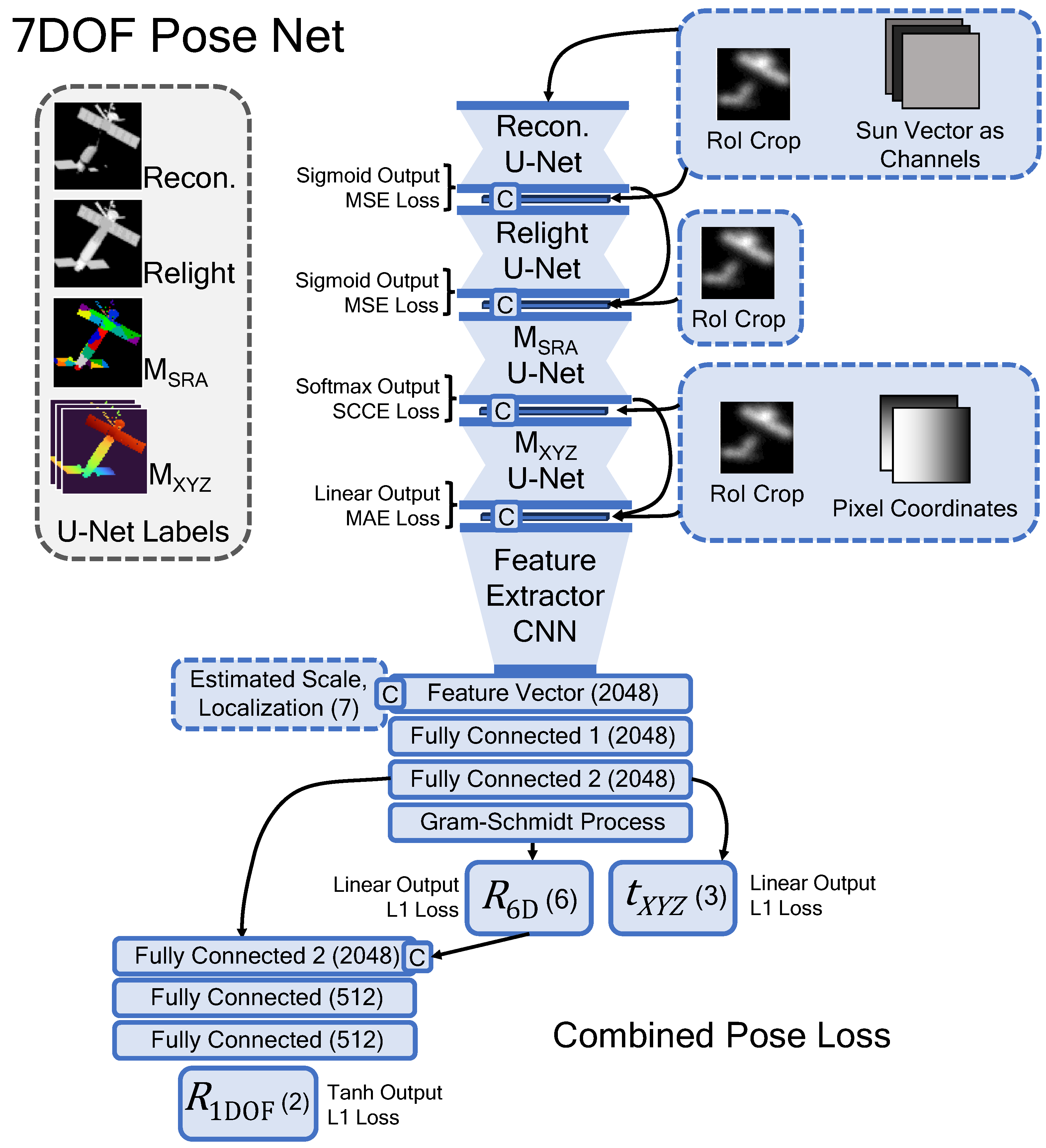
Figure 18.
Diagram showing the architecture of the seven degrees of freedom (7DOF) network, extendable to n-DOF with additional branches. For comparison, the 6DOF architecture is displayed in Figure 16.
Figure 18.
Diagram showing the architecture of the seven degrees of freedom (7DOF) network, extendable to n-DOF with additional branches. For comparison, the 6DOF architecture is displayed in Figure 16.
2.6. Inference, Temporal Filtering, and Range Post-Processing
Full frames pass through the localizer, RoI crop, and PoseNet. An adaptive multi-parameter Extended Kalman Filter (EKF) smooths (i) localizer outputs prior to cropping and (ii) PoseNet outputs post-regression, improving temporal stability without significant added latency (the pipeline ran inference at 7.1 Hz regardless of whether Kalman filtering was enabled). Range post-processing follows the training prior on combined uncertainty (tleTLE, IFOV, CAD): use the predicted scale when uncertainty is high, clip prediction to of the input estimate (the training range) when moderate, or trust the prior when low. In practice, the CAD model is likely the dominant source of uncertainty, and this bias can be corrected either dynamically by scaling the CAD size using the ratio of the prior range estimate to the predicted range, or permanently by updating the CAD geometry once sufficient data on systematic discrepancies between priors and predictions has been collected. The disparity between and Z errors is expected for this application: a ∼1 px image-space error implies ∼10 cm error but ∼10 km Z error at km and 100 nrad IFOV [18].
2.7. Evaluation Datasets and Metrics
Three sources are used: (1) LFID synthetic test set ( unique samples) generated with the same process as for training; (2) HFWO synthetic test set hold-outs produced with DIRSIG+HCIPy as described; and (3) real AO imagery. Metrics follow [5]: rotation via quaternion distance (deg); image-plane translation as two-axis angular error (nrad) or as pixel error on the frame or in meters; and range in kilometers or as relative error (%). Unless otherwise stated, evaluations use the coupled pipeline (Section 2.5.2); decoupled ablations are displayed in Figure 19.
2.8. Key Approach Adaptations
Architecturally, the 6DOF PoseNet (Figure 16) introduced several key adaptations beyond GDR-Net [5]. The model incorporates a TLE-derived range estimate and illumination vector, improving performance. Normalization was adapted for ∼1,000 km target ranges. An auxiliary localization vector was injected at the pose head to refresh memory, reducing reliance on high spatial frequency features surviving backbone propagation. Image reconstruction and relighting subnetworks were added to better handle degraded imagery. A serial backbone of four smaller U-Nets replaced the single large ResNet-34 backbone in [5], improving stability under degraded conditions by progressing from simpler tasks (denoising, deblurring) to more complex ones (deshadowing, classification, regression), and enabling efficient convergence on a single NVIDIA A100 graphics processing unit (GPU). A coupled training pipeline passed predictions from a custom Coarse Localizer (Figure 14) directly into the pose model, preserving correlations between localizer performance and image quality. To handle articulating satellites, a branched regression head and symmetry-aware loss extended the GDR-Net framework beyond 6DOF without necessitating additional model/object instances.
2.9. Implementation
Tooling includes Blender/EEVEE, Astropy, SciPy, Albumentations, TensorFlow/Keras, and HCIPy which are all well-documented and publicly available. Training was conducted on a single NVIDIA A100 GPU. The HCIPy implementation closely follows [29]. The specific CAD models used in this work are property of a third party and cannot be distributed, though equivalent-quality CAD models of HST are freely available [40]. As described, the model architecture is adapted from GDR-Net [5] which is available [7,41], and the modifications are described in detail here and in [18]. The authors acknowledge Research Computing at the Rochester Institute of Technology for providing computational resources and support that have contributed to the research results reported in this publication [42].
3. Results
3.1. Real Imagery Results (Seasat and HST)
3.1.1. Seasat (Framewise Inference)
The pipeline was evaluated on 137 manually labeled real Seasat images (see [18] for details on data and labeling), processed fully independently without Kalman filtering. Table 1 summarizes performance; pose prediction overlays are shown in Figure 20. The model achieved a mean rotation error of 5° and a mean two-axis image-plane translation error of 21 cm across the full dataset. These numerical results include unknown uncertainty from label noise, while the overlays provide a qualitative visualization of accuracy.
3.1.2. Qualitative Evaluation on Seasat (Framewise Inference)
Air Force Research Laboratory (AFRL) evaluated 250 additional real Seasat images (randomly sampled from >10,000 collected over nine years at one site). Frames were processed independently with a prior architecture variant (lacking reconstruction/relighting U-Nets and illumination vector input). To avoid the challenge of accurate manual labeling for this additional data, we introduce the Satellite Pose Alignment Rating Scale (SPARS). SPARS is a five-level qualitative metric defined with visual examples in Figure 21; the resulting score distributions are shown in Figure 22 and Table 2. The mean SPARS score across all 250 images was 3.90; below 30° elevation (unseen during training) the mean was 2.90 (), versus 4.16 at ≥30° (). Aggregated, 78.4% achieved high-confidence or ground-truth-equivalent ratings (SPARS 4–5), with only 14% falling into SPARS 1–2 (71% of those at °). These outcomes align with the framewise results above and reinforce robustness to real operational variability.
3.1.3. Hubble Space Telescope (7DOF, Framewise Inference)
HST presents greater difficulty than Seasat due to strong symmetry and a solar-array rotation. Although HST has up to 13DOF including solar arrays, aperture door, and high-gain antennae, it is simplified to 7DOF here based on image fidelity (antennae are unresolved) and the assumptions that the aperture door remains open and the solar arrays articulate in unison. A single published frame [46] yielded 2.6° rotation error and 11 cm translation error (160 nrad at the cited range); the symmetry-adjusted solar array angle error was 8° (Figure 23). On an unreleased 249-frame pass processed independently (no filtering), the body rotation error had mean of 27.1° (median 6.4°), while mean image-plane translation error was 54 cm (median 41 cm). Restricting to elevation >30° did not meaningfully affect these statistics. Complete metrics are reported in Table 3.
3.1.4. Hubble Space Telescope (Kalman Filtered)
Applying real-time Kalman filtering to the same 249-frame pass reduced mean body-rotation error from 27.1° to 5.9° (median 6.4°→4.3°). Mean image-plane translation error decreased from 54 cm to 48 cm (median 41 cm→37 cm). Mean solar-array rotation error (symmetry-adjusted) improved from 19° to 6° (median 13°→5°). Complete metrics are reported in Table 3. Error traces are shown in Figure 24 (body) and Figure 25 (array).
3.2. HFWO Synthetic Results and Image-Quality Dependence (DIRSIG+HCIPy)
This subsection consolidates pose model HFWO accuracy and its dependence on atmosphere/image quality. All numbers below use independent-frame inference unless otherwise stated. Summary tables for Seasat, ARGOS, and HST appear in Table 4, Table 5 and Table 6. Trends with adaptive optics image quality (AO-IQ) are visualized in Figure 26. AO-IQ is calculated with the General Image-Quality Equation (GIQE) v3.0 [18,47,48].
A comment is warranted on the apparent discrepancy between qualitative results showing excellent silhouette alignment (Figure 27) and quantitative errors (Figure 28b). The large rotational errors are caused by 180° ambiguities inherent to geometrically symmetric satellites like ARGOS and HST, a weakness intentionally probed by the Sim2Sim domain gap (Section 2.4). This challenge also manifests for real imagery (Figure 24 and Figure 25). While higher-resolution imagery or use of context clues (such as assuming a nominal sun-tracking orientation for the solar arrays) can mitigate this, time-series analysis provides another solution. For instance, Kalman filtering resolved the main body ambiguity for HST, though it was insufficient for the more difficult solar array symmetry. These ambiguities are challenging for human analysts as well and are a key direction for future research, with a full discussion available in [18].
3.2.1. Seasat
For cm the mean rotation error was 8.4° and the mean two-axis image-plane translation error was 323 nrad (34 cm) (Table 4), in line with the model performance on real data. Accuracy improves nearly monotonically with AO-IQ (Figure 26 and Table 4). For equivalent atmospheres the Seasat model provides improved accuracy relative to the ARGOS (smaller, highly symmetric) and HST (7DOF, symmetric) models, illustrating that Seasat’s large size and strong geometric asymmetry make it an ideal target for pose estimation.

Table 4.
Image quality and pose estimation error metrics for Seasat as a function of . Higher values correspond to reduced atmospheric turbulence and improved image quality, as reflected by increasing AO-IQ and Signal-to-Noise Ratio (SNR). Pose estimation accuracy improves with image quality, showing reduced rotation, translation, and range errors. All values are means computed over 200 hfwoHFWO synthetic test images.
Table 4.
Image quality and pose estimation error metrics for Seasat as a function of . Higher values correspond to reduced atmospheric turbulence and improved image quality, as reflected by increasing AO-IQ and Signal-to-Noise Ratio (SNR). Pose estimation accuracy improves with image quality, showing reduced rotation, translation, and range errors. All values are means computed over 200 hfwoHFWO synthetic test images.
| (cm) | AO-IQ | SNR | Rot. Err. (°) | Trans. Err. (nrad) | Trans. Err. (cm) | Range Err. (km) | Range Err. (%) |
|---|---|---|---|---|---|---|---|
| 2.5 | 3.82 | 7.08 | 115 | 1630 | 170 | 18.5 | 1.79 |
| 3.5 | 4.38 | 9.23 | 60.2 | 746 | 77.0 | 16.1 | 1.56 |
| 4.0 | 4.64 | 10.8 | 35.5 | 537 | 57.2 | 15.0 | 1.45 |
| 4.5 | 4.90 | 12.2 | 23.4 | 458 | 47.8 | 13.0 | 1.26 |
| 5.0 | 5.38 | 13.5 | 14.4 | 379 | 39.6 | 12.9 | 1.25 |
| 6.0 | 5.51 | 15.8 | 8.35 | 323 | 34.0 | 14.6 | 1.42 |
| 7.0 | 5.93 | 17.8 | 7.69 | 296 | 30.3 | 14.0 | 1.36 |
| 7.5 | 6.27 | 18.8 | 6.28 | 295 | 31.0 | 12.9 | 1.25 |
| 8.5 | 6.36 | 20.5 | 5.51 | 296 | 31.1 | 14.7 | 1.43 |
| 10.0 | 6.81 | 22.7 | 6.09 | 277 | 28.6 | 12.9 | 1.26 |
3.2.2. ARGOS
ARGOS presents strong apparent symmetry (Figure 28a), making it a much more challenging test target than Seasat (and perhaps more representative of modern LEO satellite geometries). For cm the raw mean rotation error was 66.6° and the mean image-plane translation error was 350 nrad (40 cm). Symmetry-adjusted mean rotation error was 11.6° (Table 5). Qualitative overlays show excellent silhouette alignment despite large raw rotation errors (Figure 27); the error histogram concentrates near 0°/180° (Figure 28b). The Sim2Sim domain gap presented significant challenge: replacing DIRSIG object planes with Blender object planes (same HCIPy PSFs, cm) reduced raw/adjusted rotation errors from 66.6°/11.6° to 17.2°/6.3° and translation error from 350 nrad to 276 nrad.
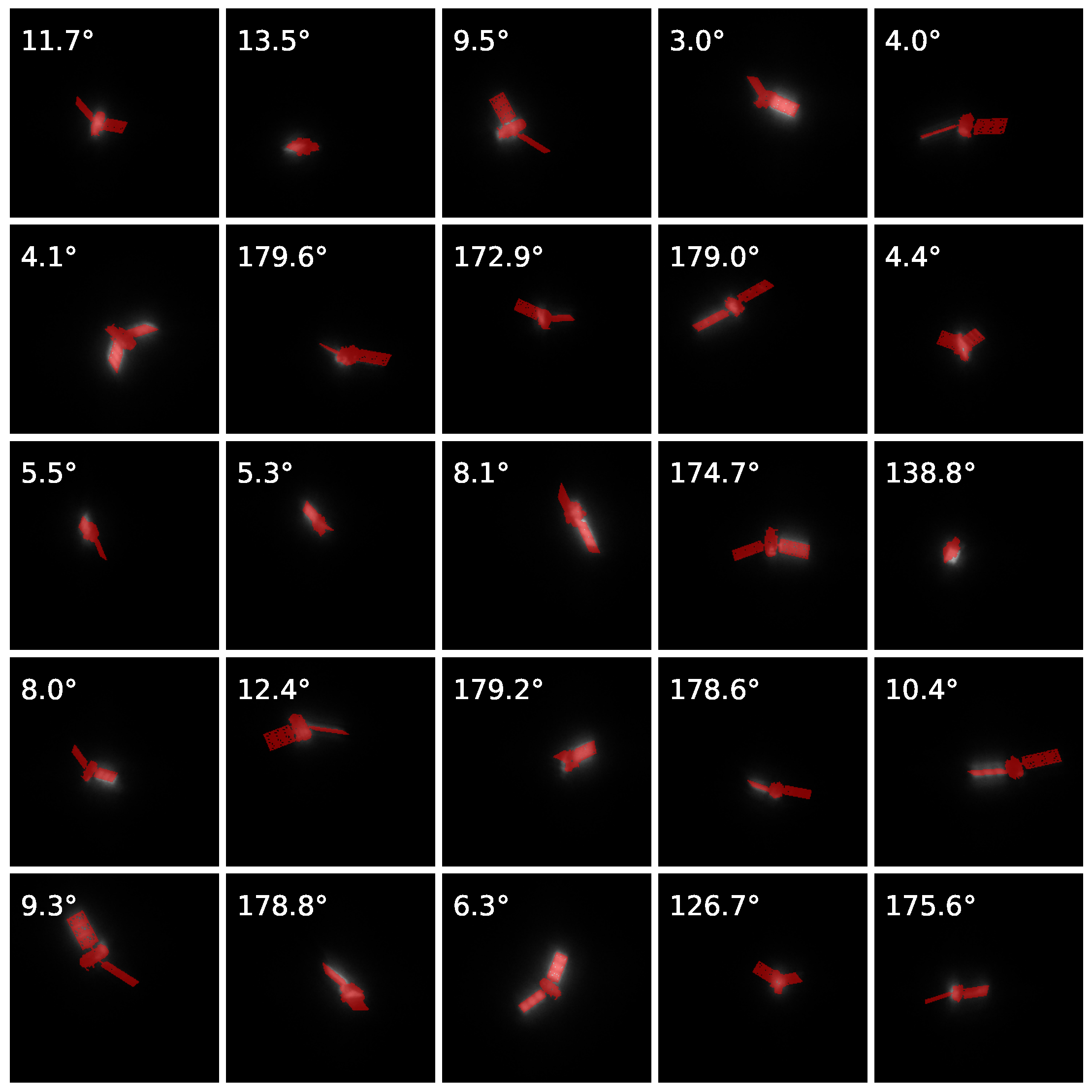
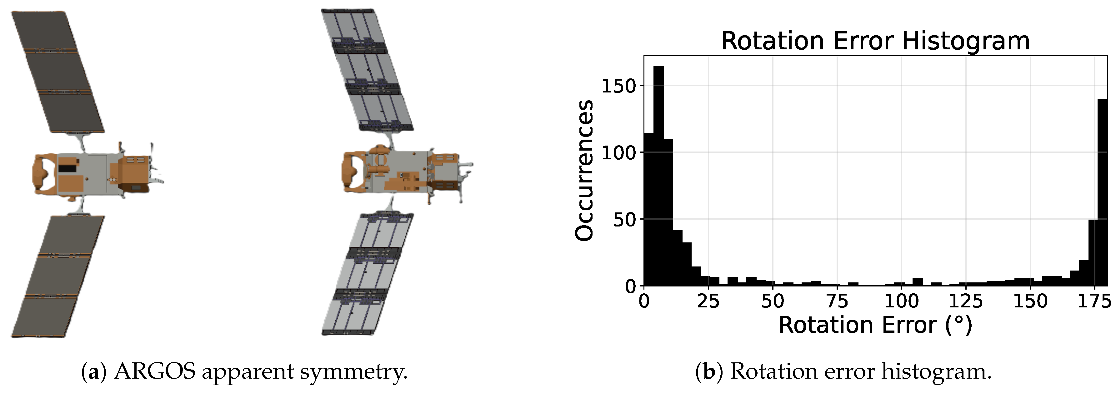
Figure 27.
Twenty-five HFWO ARGOS test images with cm displayed in grayscale, and renders produced with the pose model estimates overlaid as red wireframes. Rotation errors are shown overlaid at the upper-left of each image.
Figure 27.
Twenty-five HFWO ARGOS test images with cm displayed in grayscale, and renders produced with the pose model estimates overlaid as red wireframes. Rotation errors are shown overlaid at the upper-left of each image.
Figure 28.
(a) Two views of opposing sides of the ARGOS satellite CAD model. With the exception of small components not clearly visible under reduced contrast at high spatial frequencies, the silhouettes are nearly identical. (b) Histogram of rotation errors (in degrees) for ARGOS, with a significant cluster near 180° indicating symmetry as a primary source of error.
Figure 28.
(a) Two views of opposing sides of the ARGOS satellite CAD model. With the exception of small components not clearly visible under reduced contrast at high spatial frequencies, the silhouettes are nearly identical. (b) Histogram of rotation errors (in degrees) for ARGOS, with a significant cluster near 180° indicating symmetry as a primary source of error.
Table 5.
Image quality and pose estimation error metrics as a function of for the satellite ARGOS. Pose estimation accuracy improves with image quality, showing reduced rotation, translation, and range errors. All values are means computed over 200 HFWO test images. Rotation errors are presented both in raw and symmetry-adjusted form.
Table 5.
Image quality and pose estimation error metrics as a function of for the satellite ARGOS. Pose estimation accuracy improves with image quality, showing reduced rotation, translation, and range errors. All values are means computed over 200 HFWO test images. Rotation errors are presented both in raw and symmetry-adjusted form.
| (cm) | AO-IQ | SNR | Rot. (°) | Rot. Adj. (°) | Trans. (nrad) | Trans. (cm) | Range (km) | Range (%) |
|---|---|---|---|---|---|---|---|---|
| 5 | 5.42 | 12.2 | 77.5 | 15.9 | 472 | 53.7 | 17.3 | 1.55 |
| 6 | 5.99 | 14.7 | 66.6 | 11.6 | 350 | 40.3 | 15.9 | 1.42 |
| 7 | 5.98 | 17.2 | 61.3 | 9.4 | 331 | 37.7 | 15.6 | 1.40 |
| 10 | 7.04 | 22.6 | 56.8 | 6.8 | 302 | 34.5 | 15.8 | 1.42 |
3.2.3. Hubble Space Telescope (7DOF)
At cm the HST achieved 26.5° mean body-rotation error, 11.8° symmetry-adjusted body-rotation error, 87 cm mean image-plane translation error, and 14.7° mean solar-array angle error (Table 6). Overlays again show good silhouette alignment with symmetry-driven ambiguity (Figure 29, Figure 30a); the rotation-error histogram exhibits peaks near 0°/180° (Figure 30b). Errors decrease with and AO-IQ.
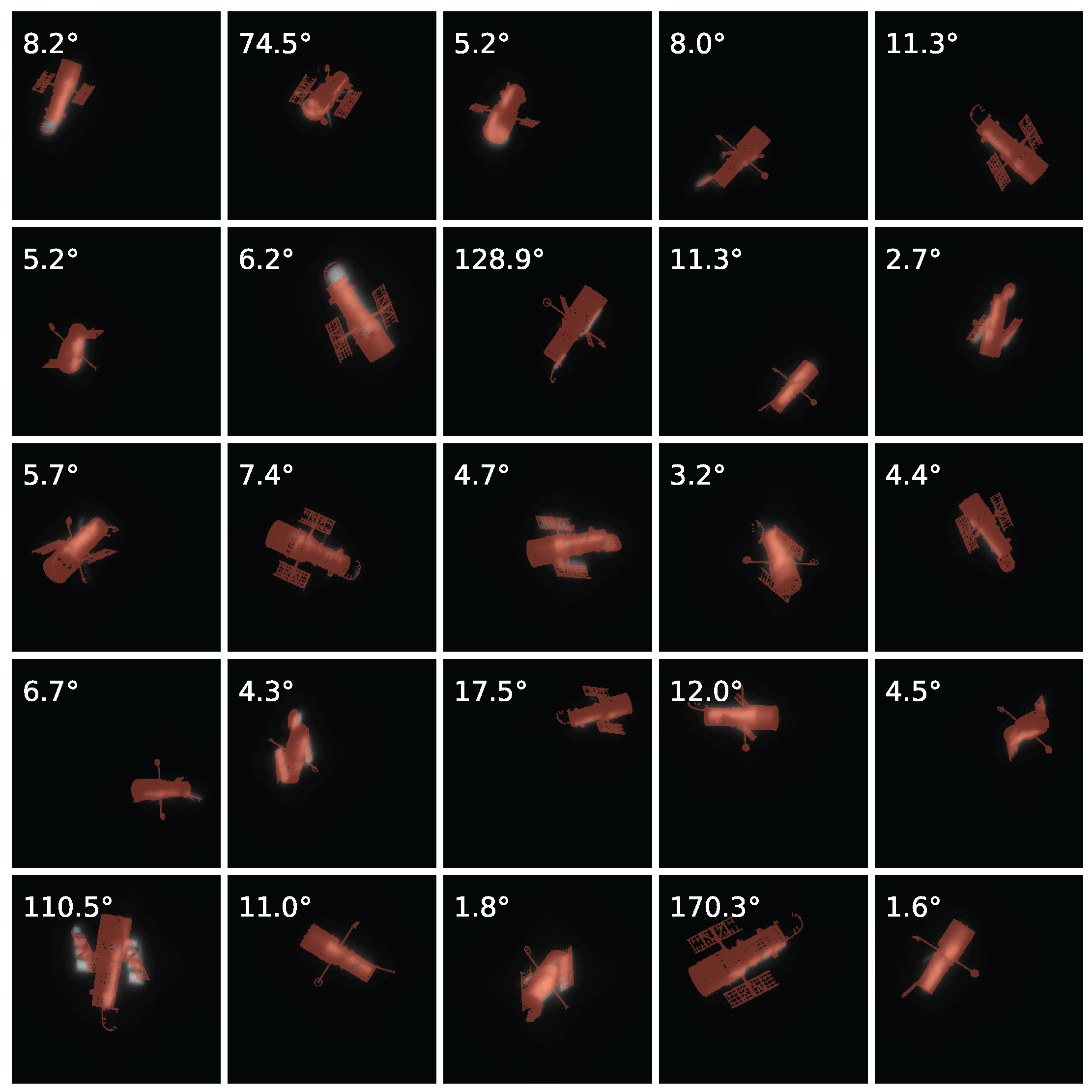
Figure 29.
Twenty-five HFWO HST test images with cm displayed in grayscale, and renders produced with the pose model estimates overlaid as red wireframes. Rotation errors are shown overlaid at the upper-left of each image.
Figure 29.
Twenty-five HFWO HST test images with cm displayed in grayscale, and renders produced with the pose model estimates overlaid as red wireframes. Rotation errors are shown overlaid at the upper-left of each image.
Table 6.
Image quality and pose estimation error metrics as a function of for the HST with 7DOF total (including solar-array rotation). Means over 200 test images; rotation errors also shown in symmetry-adjusted form.
Table 6.
Image quality and pose estimation error metrics as a function of for the HST with 7DOF total (including solar-array rotation). Means over 200 test images; rotation errors also shown in symmetry-adjusted form.
| (cm) | AO-IQ | SNR | Rot. (°) | Rot. Adj. (°) | Trans. (nrad) | Trans. (cm) | Range (km) | Range (%) | Array (°) | Array Adj. (°) |
|---|---|---|---|---|---|---|---|---|---|---|
| 5 | 5.85 | 15.68 | 37.3 | 14.5 | 1262 | 92.2 | 10.9 | 1.48 | 103.3 | 21.4 |
| 6 | 6.22 | 18.33 | 26.5 | 11.8 | 1186 | 86.6 | 11.2 | 1.52 | 102.1 | 14.7 |
| 7 | 6.64 | 20.31 | 24.8 | 11.1 | 1170 | 85.4 | 10.4 | 1.41 | 105.1 | 15.6 |
| 10 | 7.21 | 25.10 | 20.1 | 7.3 | 1100 | 80.1 | 10.9 | 1.49 | 107.6 | 12.1 |
3.2.4. Dependence on Atmosphere and Image Quality
Across satellites, pose accuracy increases with and AO-IQ. After averaging errors over pose and illumination for Seasat, AO-IQ explains nearly all remaining variance in rotation and image-plane translation error; exponential fits to mean error vs. mean AO-IQ achieve (rotation) and (translation) (Figure 26). These relationships allow forecasting of expected accuracy from image-quality proxies while remaining agnostic to specific AO hardware. Alternatively, expected accuracy (specific to a single AO system) can be forecast from atmospheric parameters.
3.3. Pose Accuracy vs. Object Pose
To isolate orientation effects, a single AO PSF ( cm) and realistic noise were applied (via HCIPy) to all 11,000 pristine Seasat LFID test renders, holding image quality fixed. To determine if the model struggles with specific viewing angles, we grouped the images into distinct orientation categories. Using ground-truth rotations, unsupervised k-medoids clustering (quaternion distance) partitioned the 3DOF orientation space into 110 pose classes (mean intraclass quaternion distance °, interclass °; images/class).
Analyzing these classes revealed that estimation accuracy depends heavily on the target’s pose. Class-mean rotation errors spanned °–° (global mean °), with an interclass standard deviation of ° (coefficient of variation (CV) ), indicating substantial pose-dependent difficulty, though intraclass variability remained high (mean intraclass std dev °). Translation estimation showed a more moderate dependence on pose (class means 21–72 cm; global mean 33 cm; CV ; mean intraclass std dev 28 cm), while range estimation exhibited the weakest dependence (class means – km; global mean km; CV ; mean intraclass std dev km).
Physically, accuracy was poorest when Seasat was oriented with the solar arrays closer to the sensor, obscuring portions of the satellite body behind them. In contrast, accuracy was highest with Seasat oriented with the synthetic-aperture radar (SAR) panels towards the top of the image, the solar arrays towards the bottom of the image, and the boom antennas projecting towards the right of the image, as shown in Figure 31.
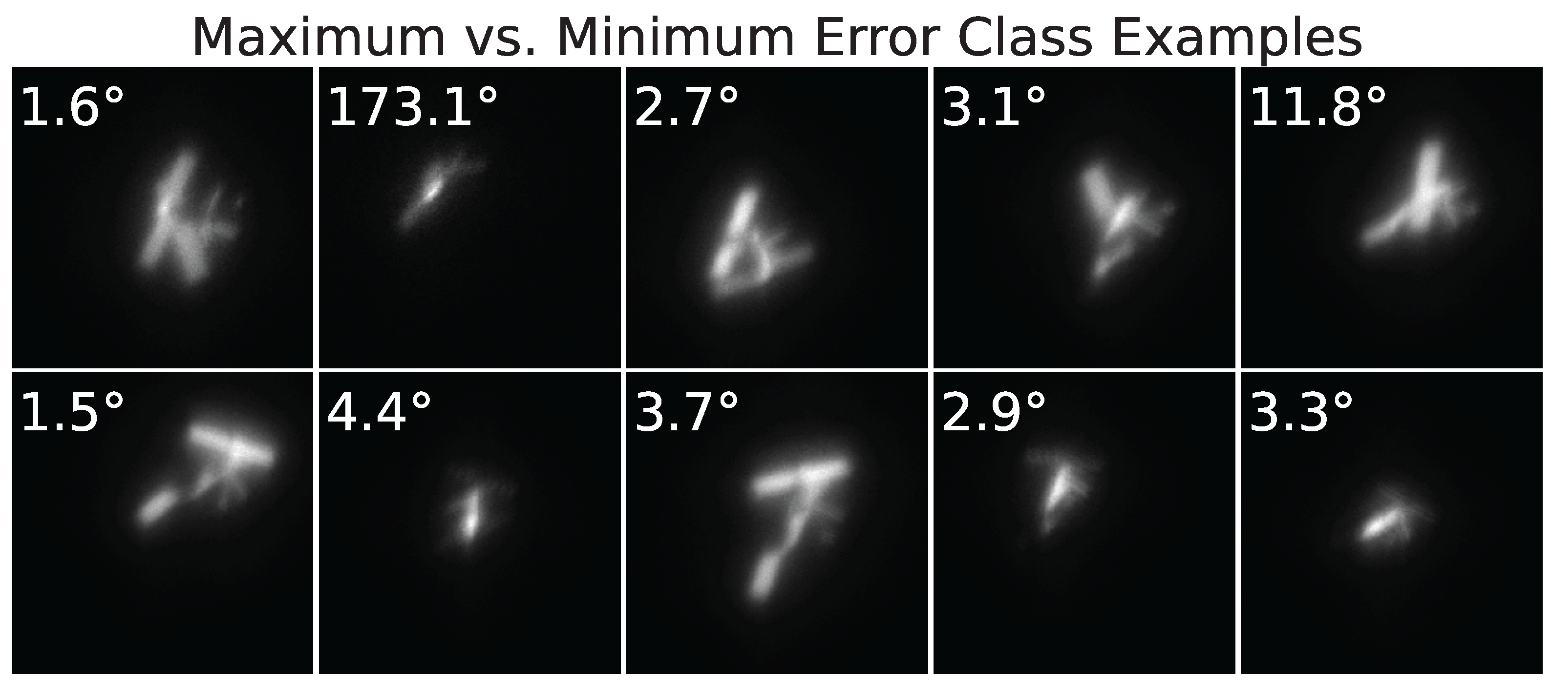
Figure 31.
The first row displays five test images from the pose class with the maximum mean rotation error, with per-sample rotation errors overlaid at the upper left of each test image. The second row displays five test images from the pose class with the minimum mean rotation error.
Figure 31.
The first row displays five test images from the pose class with the maximum mean rotation error, with per-sample rotation errors overlaid at the upper left of each test image. The second row displays five test images from the pose class with the minimum mean rotation error.
3.4. Pose Accuracy vs. Illumination Direction
Using the same 11,000-image set, illumination orientations (in image coordinates: right, up, out of the image) were clustered into 110 classes. Rotation error exhibited a strong dependence on lighting: global mean ° with class means from ° to ° (std dev of class means °, CV; mean intraclass std dev °). Translation showed a modest dependence (means 23–57 cm; global mean 33 cm; CV), and range was weakly affected (means – km; global mean km; CV). A significant correlation was found between rotation error and the illumination Z-component (Pearson , ): back-illumination () increased error, while front-illumination () reduced error, as shown in Figure 32. Further analyses are provided in [18].
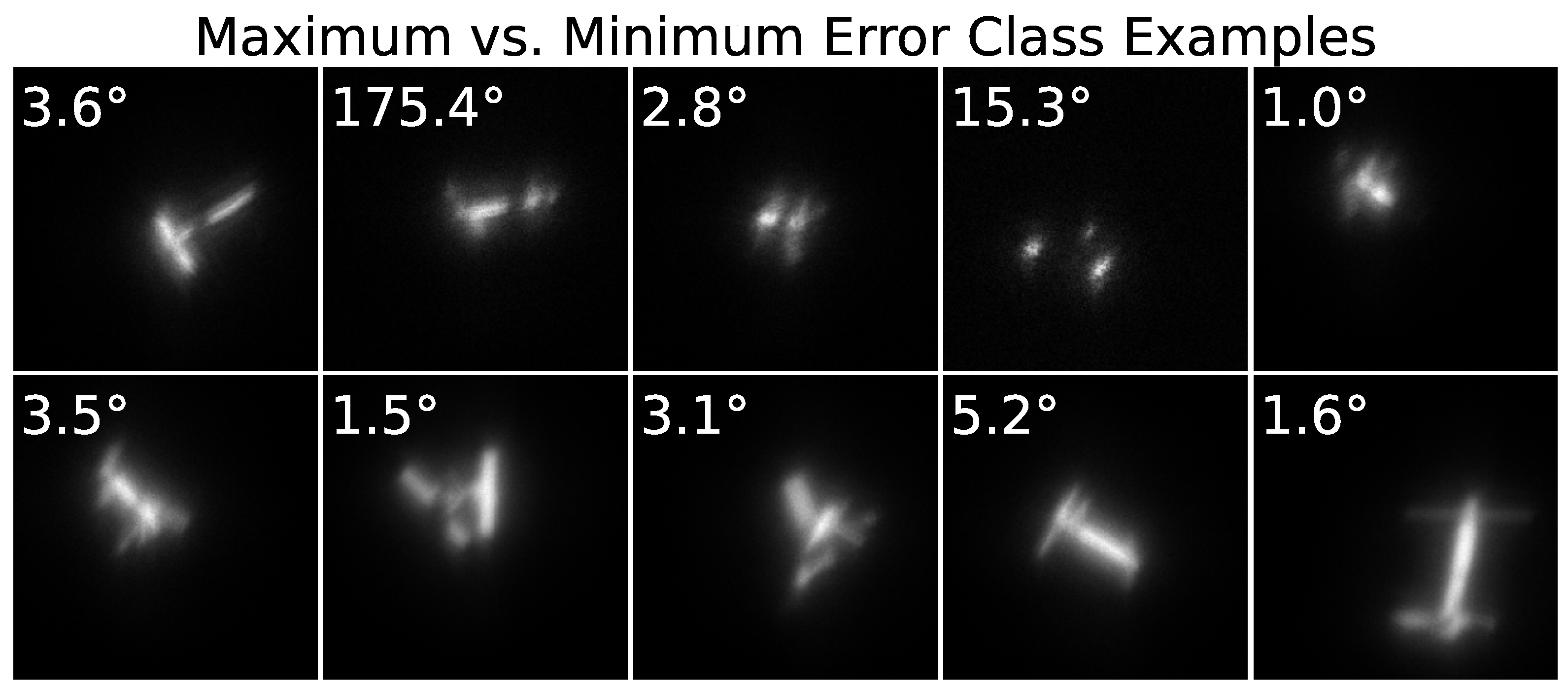
Figure 32.
The first row displays five test images from the illumination direction class with the maximum mean rotation error, with per-sample rotation errors overlaid at the upper left of each test image. The second row displays five test images from the illumination direction class with the minimum mean rotation error.
Figure 32.
The first row displays five test images from the illumination direction class with the maximum mean rotation error, with per-sample rotation errors overlaid at the upper left of each test image. The second row displays five test images from the illumination direction class with the minimum mean rotation error.
3.5. Pose Accuracy vs. CAD Fidelity
Four independent Seasat training sets captured geometry/material realism at increasing fidelity: (i) 100-triangle, single material; (ii) 729-triangle, 15 materials (decimated); (iii) full-fidelity 34k-triangle, 17 materials; (iv) full-fidelity with randomized material augmentation (Figure 33). Each Coarse Localizer/PoseNet was trained identically and evaluated on 2,000 HFWO test images. Mean rotation/translation errors improved monotonically with fidelity: 77.8°/689 nrad (100 tri) → 54.9°/617 nrad (729 tri) → 46.5°/569 nrad (34k tri) → 42.4°/537 nrad (34k+mat-aug). The model degrades gracefully under reduced CAD realism. Additional detail is available in [18].
3.6. Pose Accuracy vs. Training Set Size
The full 264k-sample training set (88k unique poses, 3× randomized augmentations) was subsampled to 16k, 32k, 64k, 88k, and 176k; the pose model was retrained per subset while keeping the localizer fixed (trained on 264k). All models were evaluated on the same 2,000-image HFWO test set used in Section 3.5. Mean errors (averaged across 10 atmospheres) improved with dataset size: rotation decreased from 73.4° (16k) to 42.4° (264k), translation from 867 nrad to 537 nrad, and range from 16.2 km to 14.5 km. An exponential decay fit to rotation error vs. dataset size achieved ; extrapolation to 1.264M samples projects ° mean rotation error, indicating continual (but diminishing) improvement. Additional details are provided in [18].
3.7. Human Analyst Comparison
A benchmark was conducted on 200 Seasat HFWO test images at cm (shorter simulated integration time, ∼50% lower SNR than Section 3.2.1). Frames were processed independently without temporal context by both a human labeler (the first author, using a custom graphical user interface (GUI) detailed in [18]) and the pose model. Cumulative error distributions are shown in Figure 34.
Rotation: The mean human rotation error was 66.6°, whereas the model achieved 34.4°, outperforming the analyst on 141/200 images. Rotation errors ranged from 0.6° to 180.0° for the human and from 0.3° to 177.0° for the model.
Translation: The mean absolute two-axis image plane angular translation error was 572 nrad (59.3 cm) for manual labeling and 473 nrad (48.3 cm) for the model, with the model outperforming the analyst on 116/200 images. Translation errors ranged from 54 to 3812 nrad for the human and from 27 to 2003 nrad for the model. Range was not manually labeled, and the same range estimate provided to the model for inference was used to render the labeling GUI.
Throughput: Manual labeling required 6.27 h in total (mean 1 min 43 s per image; range 23 s to 8 min 37 s). Model inference at 7.1 Hz on a RTX 3060 GPU processed the same set in 28 s ( faster).
3.8. Approach Practicality, Runtime, and Hardware Requirements
A key aim of this research effort was operational practicality. Training data were synthesized with Blender and Python tooling (RTX3060 GPU, 6GB VRAM; 32GB RAM). Model training and augmentation ran on a single NVIDIA A100 (40 GB VRAM) [42]. Rendering 110k grayscale images plus paired front-lit views required ∼10.5 h; rendering added ∼2.5 h. Data loading/preprocessing and augmentations contributed ∼3.3 h total (CPU). A100 training required ∼8.5 h for the Coarse Localizer, h for the complete PoseNet backbone, and ∼3.5 h for the pose head. With early stopping (50-epoch caps; patience 10), the full process (including data generation) required <40 h. Many stages (rendering, augmentation, RoI crops) are trivially parallelizable and could be distributed to reduce wall time further. Pretrained backbones or transfer learning were not used but could likely shorten training.
The storage footprint per satellite was ∼25 GB (lossless compression), dominated by ∼18 GB for 286k augmented 16-bit images; weights were ∼100 MB (Coarse Localizer) and ∼350 MB (pose network). At inference, the end-to-end pipeline (localizer → RoI crop → PoseNet → optional EKF) sustained Hz in real-time streaming mode on the RTX3060, ingesting frames sequentially with batch size.
3.9. Utility of Generalized Models for SDA
We assessed several large, generalized models on SDA tasks: OpenAI and Google Gemini VLMs for monocular pose and Depth AnythingV2 for monocular depth. Tests used pristine orthographic renders (512×512 px) and required pose estimates reletive to a reference view.
3.9.1. Vision-Language Models
OpenAI’s GPT-4o (gpt-4o-2024-11-20) performed poorly on rotation and translation: (i) relative 3DOF rotation from two views: correct across two setups; (ii) one degree of freedom (1DOF) rotation classification with 10 classes: correct (≈ chance); (iii) 1DOF translations along X or Z: all incorrect. A heavily simplified 1DOF Z-axis rotation was answered correctly times, with one success occurring only after corrective feedback. A March 2025 GPT-4o update [49] improved a single simplified case: with baseline/target embedded as red/blue channels, the model identified the axis and direction of 1DOF X translation in trials, though magnitudes varied without a scale reference. Prompts, input images, and complete experimental procedures are provided in [18].
OpenAI’s o4-mini-high (April 2025) showed materially better but still limited capability [50,51]. With pixel scale provided, it recovered 1DOF X translations with correct axis/direction in all trials and near-metric accuracy (red/blue overlay: –m for a 5 m truth; separate images: 5.00 m in all three trials). For 1DOF Z translation (separate images), it correctly inferred a twofold distance change (). On the 10-class 1DOF rotation benchmark it reached correct (43.3%), with strong Z-axis (image-plane rotation) results () but weak X/Y (out-of-plane rotation) ( and ). A simple 6DOF task with multi-view context remained unsolved (three incorrect attempts).
Google’s Gemini Pro 3.1 Preview (March 2026) [52] continued the trend of improved performance, achieving perfect performance on the 1DOF Z translation and 1DOF X translation (separate images) tasks. Notably, while o4-mini-high also performed perfectly on these tasks it did so with extensive use of Python for calculations (such as centroiding) within the chain-of-thought, despite being instructed not to in the prompt. All tool use was explicitly disabled for Gemini Pro 3.1 Preview, so performance was purely the result of the multimodal model ingesting and operating on tokenized images. Gemini Pro 3.1 Preview also achieved a perfect score on the 10-class 1DOF rotation benchmark. The prompts were modified, appending "The first image is the baseline pose", as Gemini Pro 3.1 Preview does not access the filenames of uploaded images and it was important that the model correctly distinguish the baseline reference pose from the target pose so that the predicted transformations were not inverted. The model consistently identified transformations about the X, Y, and Z axes, suggesting a more robust internal representation of 3D geometry. Inference times (driven mainly by number of reasoning iterations) varied significantly with apparent task complexity, from under 10 seconds to over two minutes. The model’s capabilities with degraded imagery or on more challenging, unconstrained 6DOF pose estimation tasks remain to be tested. In a highly simplified 6DOF pose test Gemini Pro 3.1 Preview improved on o4-mini-high with correct rotations and correct translations (o4-mini-high had zero correct rotations or translations). See [18] Sec. 9.1.8, “6DOF Pose Estimation with Context” for complete details.
While VLMs are progressing rapidly, they still require tens to hundreds of seconds of reasoning and remain limited to pose problems that are narrowly constrained with pristine data. This investigation is not intended as a comprehensive benchmark, and many VLMs were not evaluated (including OpenAI’s latest model), as that is outside the scope of this work. Rather, these results highlight the clear trend of improvement (a trend also reflected in broader industry benchmarks evaluating general spatial and object understanding [53]) and motivate the need for a formal, standardized pose estimation benchmark for generalized models.
3.9.2. General-Purpose Monocular Depth
Depth Anything V2 [54], trained at web scale (including ImageNet-21k classes such as satellite/space_station [55]), produces credible depth on everyday scenes but failed to recover meaningful structure on simulated SDA imagery of Seasat. A domain-specific depth model (the PoseNet backbone) performed substantially better (Figure 35) [18]. Given that these test images were in-distribution for PoseNet, its superior performance was expected. However, the severity of Depth Anything V2’s failure was unexpected given its strong cross-domain generalization and a massive training set of 595k synthetic images and ∼62M pseudo-labeled real images.
3.9.3. Takeaway
Generalized models did not provide reliable pose or depth estimation for SDA without task-specific conditioning. Limited successes occurred only in highly simplified settings with explicit pixel scale or strong priors. These results motivate domain adaptation and targeted benchmarks before generalized models can replace specialized SDA computer vision pipelines.
4. Discussion
This work delivers and validates the first practical end-to-end pipeline for real-time, ≥6DOF satellite pose estimation from ground-based AO imagery, trained exclusively on synthetic data. The system generalizes well to real imagery: Seasat achieves ° mean rotation error and 21 cm mean image-plane translation error without temporal filtering, and a full HST pass improves from 27.1° framewise error to 5.9° with Kalman filtering. A qualitative evaluation of 199 additional Seasat frames rated 89.4% of predictions as “ground-truth equivalent” or “high confidence” (Section 3.1.2). On a high-fidelity synthetic test set (HFWO, cm), the model attains 8.4° mean rotation and 34 cm mean image-plane translation error, consistent with real-image results. Operational viability is confirmed: end-to-end inference runs at 7.1 Hz on consumer hardware and outperforms human labeling by 48.4% in mean rotation error while operating faster (Figure 34). Finally, we establish quantitative, operationally useful baselines linking performance to atmospheric conditions: a single scalar image-quality metric (AO-IQ) explains of the variance in both rotation and translation error for Seasat after controlling for object pose and illumination direction (Figure 26).
4.1. Interpretation of Results in Context
This work advances beyond prior art ([3,4]) by enabling full ≥6DOF pose inference under realistic imaging conditions, validated on real imagery. Key, application-specific architectural adaptations from GDR-Net include:
- Serial backbone: four smaller U-Nets (reconstruction → relighting → segmentation → pose) stabilize training and improve robustness to degraded inputs, while remaining single-GPU trainable (Section 3.8, Figure 16).
- Physical priors: injecting illumination direction and TLE-derived range estimates improves accuracy.
- Coupled training: training the PoseNet on the Coarse Localizer outputs reduces tail errors from poor image quality (29% improvement in 90th-percentile error, Figure 19).
Additional adaptations include target range reparameterization (suitable for ranges of ∼1,000 km), auxiliary localization inputs at the feature level, main body pose-aware branched regression heads for articulating components, and a tailored data augmentation pipeline randomized over blur, noise, and other SDA AO-specific degradations ([19], Section 2.3.4). These design choices enable performant generalization to unseen AO data and extension to 7DOF pose estimation (Figure 18).
4.2. Key Challenges and Limitations
Remaining limitations include both algorithmic and practical factors:
- Symmetry ambiguities: Symmetric geometries (ARGOS, HST) drive residual error. On ARGOS at cm for HFWO testing, raw mean rotation error is 66.6°, dropping to 11.6° after symmetry adjustment (Table 5, Figure 27). Kalman filtering has the ability to substantially mitigate geometric ambiguity (Figure 24).
- Dependence on CAD fidelity: Pose accuracy degrades gracefully with decreased CAD fidelity (Section 3.5). Accurate CAD models are still required at train time. Ongoing work in automated 3D mesh generation and model-free pose estimation ([56,57]) is relevant.
- 7DOF limits: For HST, farthest point sampling semantic segmentation U-Net output labels were insufficient to guide learning for flat and highly symmetric components (solar array front/back). Explicit front/back surface symmetry-breaking supervision is a recommended future direction (Figure 25). Alternatively, known illumination direction can be used to break symmetry for solar arrays.
4.3. Implications for SDA
The pipeline provides a validated approach for real-time monitoring and enhanced operator situational awareness as well as for post-processing imagery archives into pose timelines. Intermediate model outputs (, , etc.) require negligible overhead and support additional analysis. Despite advances in generalist VLMs, comprehensive testing (Section 3.9) shows these models fail on unconstrained pose tasks unless aided by internal tools (image centroiding using Python during internal chain-of-thought) and simplified settings. Specialized models remain necessary for practical SDA utility at this time.
4.4. Future Research Directions
Priority areas for further research include:
- Improved symmetry handling: Evaluate ARGOS pose model on real imagery and devise architectures and approaches more robust against strong geometric symmetry.
- Test-time refinement: A novel render-and-compare procedure [18] yields modest gains on high-quality frames (4.5° → 3.4° mean rotation error, 24 cm → 19 cm mean translation error at cm) but is ineffective on marginal imagery (where it would add the most value) and computationally impractical (5–30 s/frame). Improved test-time refinement methods could prove useful.
- Efficiency: Enable multi-target model training via satellite ID injection, implement parallel data generation, and leverage transfer learning across satellites. Improve range handling by treating TLE-range and sensor IFOV as ground truth and resizing CAD geometry accordingly. Explore more advanced pretrained backbone architectures.
- Generalized model benchmarking: Propose a public SDA or pose estimation benchmark to track VLM vs. specialized approach performance.
5. Conclusions
We present the first practical, real-time (7.1 Hz) system for estimating ≥6DOF satellite pose from resolved ground-based AO imagery, trained purely on synthetic data. The model generalizes to real targets: Seasat achieves ° mean rotation and 21 cm mean image-plane translation error without temporal filtering; HST achieves 27.1° framewise error that falls to 5.9° with Kalman filtering. Against human labeling, the system is both faster () and more accurate (48.4% lower mean rotation error). We quantify accuracy as a function of image quality, pose, and illumination; AO-IQ explains of atmosphere-driven variance for Seasat, enabling actionable performance forecasting. We extend the framework to n-DOF (7DOF demonstrated for HST) and document limits due to symmetry and CAD fidelity. Finally, we show that contemporary generalized VLMs are not yet viable substitutes for domain-specific SDA models.
This work establishes an operationally relevant baseline for automated satellite characterization from resolved imagery. By moving beyond theoretical exploration to a validated, high-performance system, it provides a scalable methodology for exploiting SDA sensor data at speed and at scale. As LEO becomes increasingly congested, such capabilities will be central to sustained situational awareness and space traffic management.
Author Contributions
Conceptualization, T.D., M.G., D.W., J.F., and D.M.; methodology, T.D., M.G., and D.W.; software, T.D. and D.F.; validation, T.D., M.G., and D.F.; formal analysis, T.D. and M.G.; investigation, T.D., D.F. and M.G.; writing—original draft preparation, T.D.; writing—review and editing, T.D., D.F., J.F., D.W., D.M. and M.G.; supervision, J.F., D.W., D.M. and M.G. All authors have read and agreed to the published version of the manuscript.
Funding
Approved for public release; distribution is unlimited. Public Affairs release approval #AFRL-2026-2757. This research was funded by the Department of Defense and Air Force Research Laboratory. The views expressed are those of the author and do not reflect the official policy or position of the US Air Force, US Space Force, Department of Defense, or the US Government.
Institutional Review Board Statement
Ethical review and approval were waived for this study. The work involved authors performing performance benchmarks and qualitative scoring of image data, a common practice in the field. The tasks posed no participant risk beyond that of normal computer use.
Informed Consent Statement
Not applicable. The only human subjects involved were the authors.
Data Availability Statement
The datasets presented in this article are not readily available because access is restricted due to Department of Defense and Air Force Research Laboratory policies. Requests to access the datasets should be directed to the corresponding author. Publicly releasable code and data will be shared via GitHub at https://www.github.com/twd14.
Acknowledgments
The authors would like to thank Dr. Dimah Dera, Dr. James Albano, and Dr. Linwei Wang of the Rochester Institute of Technology for their valuable guidance and expertise. We also thank our colleagues at the Air Force Research Laboratory (AFRL) for their technical expertise and many helpful discussions. The authors acknowledge Research Computing at the Rochester Institute of Technology for providing computational resources and support that have contributed to the research results reported in this publication [42].
Conflicts of Interest
The authors declare no conflicts of interest.
References
- Space Training and Readiness Command (STARCOM). SDP 3-100, Space Domain Awareness; United States Space Force Space Doctrine Publication, 2023. [Google Scholar]
- GregorDS. Six degrees of freedom — Wikipedia, The Free Encyclopedia, 2015. Adapted from the original Creative Commons Wikipedia diagram. Available online: https://en.wikipedia.org/wiki/Six_degrees_of_freedom#/media/File:6DOF.svg (accessed on 25 September 2024).
- Wood, G.E. Estimation of Satellite Orientation from Space Surveillance Imagery Measured with an Adaptive Optics Telescope. Master’s thesis, Air Force Institute of Technology, 1996. [Google Scholar]
- Lucas, J.; Kyono, T.; Werth, M.; Gagnier, N.; Endsley, Z.; Fletcher, J.; AFRL, I.M. Estimating Satellite Orientation through Turbulence with Deep Learning. Advanced Maui Optical and Space Surveillance Technologies Conference (AMOS) Conference Proceedings, 2020. [Google Scholar]
- Wang, G.; Manhardt, F.; Tombari, F.; Ji, X. GDR-Net: Geometry-Guided Direct Regression Network for Monocular 6D Object Pose Estimation. In Proceedings of the IEEE/CVF Conference on Computer Vision and Pattern Recognition (CVPR), June 2021; pp. 16611–16621. [Google Scholar]
- Li, Z.; Wang, G.; Ji, X. CDPN: Coordinates-Based Disentangled Pose Network for Real-Time RGB-Based 6-DoF Object Pose Estimation. In Proceedings of the 2019 IEEE/CVF International Conference on Computer Vision (ICCV), 2019; pp. 7677–7686. [Google Scholar] [CrossRef]
- Liu, X.; Zhang, R.; Zhang, C.; Fu, B.; Tang, J.; Liang, X.; Tang, J.; Cheng, X.; Zhang, Y.; Wang, G.; et al. GDRNPP. 2022. Available online: https://github.com/shanice-l/gdrnpp_bop2022.
- Zhang, R.; Huang, Z.; Wang, G.; Liu, X.; Zhang, C.; Ji, X. GPose2023: A Modularized Learning-based Object Pose Estimator. In Oral Presentation at the 8th International Workshop on Recovering 6D Object Pose (ICCV); Tsinghua University, BNRist, 2023. [Google Scholar]
- Sundermeyer, M.; Hodan, T.; Labbé, Y.; Wang, G.; Brachmann, E.; Drost, B.; Rother, C.; Matas, J. BOP Challenge 2022 Results Presentation. 7th International Workshop on Recovering 6D Object Pose, ECCV 2022, Tel Aviv, 2022; Available online: https://cmp.felk.cvut.cz/sixd/workshop_2022/slides/bop_challenge_2022_results.pdf.
- Hodan, T.; Sundermeyer, M.; Labbe, Y.; Nguyen, V.N.; Wang, G.; Brachmann, E.; Drost, B.; Lepetit, V.; Rother, C.; Matas, J. BOP Challenge 2023 on Detection Segmentation and Pose Estimation of Seen and Unseen Rigid Objects. In Proceedings of the Proceedings of the IEEE/CVF Conference on Computer Vision and Pattern Recognition, 2024; pp. 5610–5619. [Google Scholar]
- Zhou, Y.; Barnes, C.; Lu, J.; Research, A.; Yang, J.; Li, H. On the continuity of rotation representations in neural networks. In Proceedings of the IEEE/CVF Conference on Computer Vision and Pattern Recognition, 2019. [Google Scholar]
- Kisantal, M.; Sharma, S.; Park, T.H.; Izzo, D.; Märtens, M.; D’Amico, S. Satellite pose estimation challenge: Dataset, competition design, and results. IEEE Trans. Aerosp. Electron. Syst. 2020, 56, 4083–4098. [Google Scholar] [CrossRef]
- Park, T.H.; Märtens, M.; Jawaid, M.; Wang, Z.; Chen, B.; Chin, T.J.; Izzo, D.; D’Amico, S. Satellite Pose Estimation Competition 2021: Results and Analyses. Acta Astronaut. 2023, 204. [Google Scholar] [CrossRef]
- Park, T.H.; D’Amico, S. Robust multi-task learning and online refinement for spacecraft pose estimation across domain gap. Adv. Space Res. 2024. [Google Scholar] [CrossRef]
- Park, T.H.; D’Amico, S. Adaptive neural-network-based unscented kalman filter for robust pose tracking of noncooperative spacecraft. J. Guid. Control Dyn. 2023, 46, 1671–1688. [Google Scholar] [CrossRef]
- Park, T.H.; D’Amico, S. Bridging Domain Gap for Flight-Ready Spaceborne Vision. arXiv 2024, arXiv:2409.11661. [Google Scholar]
- Dickinson, T.; Walvoord, D.; Gartley, M. Automated 6DOF Satellite Pose Estimation from Resolved Ground-Based Imagery. Advanced Maui Optical and Space Surveillance Technologies Conference (AMOS) Conference Proceedings, 2024. [Google Scholar]
- Dickinson, T.; Dera, Dimah; Albano, James; Wang, Linwei; Walvoord, Derek; Montera, Dennis. From Sim to 6DOF: Deep Learning for Real-Time Satellite Pose Estimation from Resolved Ground-Based Imagery Advisors. Ph.d. dissertation, Rochester Institute of Technology, RIT - Main Campus, 2025. [Google Scholar]
- Drummond, J.D. Adaptive optics Lorentzian point spread function. Proc. Adapt. Opt. Syst. Technol. SPIE 1998, Vol. 3353, 1030–1037. [Google Scholar] [CrossRef]
- Abadi, M.; Agarwal, A.; Barham, P.; Brevdo, E.; Chen, Z.; Citro, C.; Corrado, G.S.; Davis, A.; Dean, J.; Devin, M.; et al. TensorFlow: Large-Scale Machine Learning on Heterogeneous Systems, 2015. Software available from tensorflow.org. [CrossRef] [PubMed]
- Astropy Collaboration; Price-Whelan, A.M.; Lim, P.L.; et al. The Astropy Project: Sustaining and Growing a Community-oriented Open-source Project and the Latest Major Release (v5.0) of the Core Package. Astrophys. J. 2022, arXiv:astro935, 167. [Google Scholar] [CrossRef]
- Adriano, A.; Scott, K.A.; Azad, N.L. Extreme Gradient Boosting and Deep Learning Models for the Classification of Synthetic Space Debris Light Curves. Advanced Maui Optical and Space Surveillance Technologies Conference (AMOS) Conference Proceedings, 2024. [Google Scholar]
- Virtanen, P.; Gommers, R.; Oliphant, T.E.; Haberland, M.; Reddy, T.; Cournapeau, D.; Burovski, E.; Peterson, P.; Weckesser, W.; Bright, J.; et al. SciPy 1.0: Fundamental Algorithms for Scientific Computing in Python. Nat. Methods 2020, 17, 261–272. [Google Scholar] [CrossRef] [PubMed]
- rd Generation Partnership Project (3GPP). Technical Specification Group Radio Access Network; Study on New Radio (NR) to Support Non-Terrestrial Networks (Release 15); Technical Report 38.811; 3rd Generation Partnership Project (3GPP), 2019. [Google Scholar]
- Ghiasi, G.; Lee, H.; Kudlur, M.; Dumoulin, V.; Shlens, J. Exploring the structure of a real-time, arbitrary neural artistic stylization network. In Proceedings of the Proceedings of the British Machine Vision Conference (BMVC), 2017. [Google Scholar]
- Google. Arbitrary Image Stylization v1, 2020. Accessed. (accessed on 2024-12-01).
- Buslaev, A.; Iglovikov, V.I.; Khvedchenya, E.; Parinov, A.; Druzhinin, M.; Kalinin, A.A. Albumentations: fast and flexible image augmentations. Information 2020, 11, 125. [Google Scholar] [CrossRef]
- Goodenough, A.A.; Brown, S.D. DIRSIG5: Next-generation remote sensing data and image simulation framework. IEEE J. Sel. Top. Appl. Earth Obs. Remote Sens. 2017, 10, 4818–4833. [Google Scholar] [CrossRef]
- Por, E. Adaptive Optics with a Shack-Hartmann Wavefront Sensor. Accessed. (accessed on 2024-11-19).
- Por, E.H.; Haffert, S.Y.; Radhakrishnan, V.M.; Doelman, D.S.; van Kooten, M.; Bos, S.P. High Contrast Imaging for Python (HCIPy): an open-source adaptive optics and coronagraph simulator. Proc. Adapt. Opt. Syst. VI. SPIE 2018, Vol. 10703, 1112–1125. [Google Scholar]
- Johnson, R.; Montera, D.; Schneeberger, T.; Spinhirne, J. A new sodium guidestar adaptive optics system for the Starfire Optical Range 3.5 m telescope. In Proceedings of the Adaptive Optics: Methods, Analysis and Applications; Optica Publishing Group, 2009; p. AOTuA1. [Google Scholar]
- Gladysz, S.; Le Louarn, M.; Yaitskova, N.; Garcia-Rissmann, A.; Kann, L.; Drummond, J.D.; Johnson, R.L.; Roskey, D. Size of the halo of the adaptive optics PSF. Proc. Adapt. Opt. Syst. III. SPIE 2012, Vol. 8447, 802–816. [Google Scholar]
- Fried, D.L. Optical resolution through a randomly inhomogeneous medium for very long and very short exposures. J. Opt. Soc. Am. 1966, 56, 1372–1379. [Google Scholar] [CrossRef]
- Tyson, R.K.; Frazier, B.W. Principles of adaptive optics; CRC press, 2022. [Google Scholar]
- Zheng, Z.; Wang, P.; Ren, D.; Liu, W.; Ye, R.; Hu, Q.; Zuo, W. Enhancing geometric factors in model learning and inference for object detection and instance segmentation. IEEE Trans. Cybern. 2021, 52, 8574–8586. [Google Scholar] [CrossRef]
- Zheng, Z.; Wang, P.; Liu, W.; Li, J.; Ye, R.; Ren, D. Distance-IoU loss: Faster and better learning for bounding box regression. Proc. Proc. AAAI Conf. Artif. Intell. 2020, Vol. 34, 12993–13000. [Google Scholar] [CrossRef]
- Ren, S. Faster r-cnn: Towards real-time object detection with region proposal networks. arXiv 2015, arXiv:1506.01497. [Google Scholar]
- Kingma, D.P. Adam: A method for stochastic optimization. arXiv 2014, arXiv:1412.6980. [Google Scholar]
- Developers, S. SciPy: Scientific Computing Tools for Python - Rotation. magnitude. Accessed. 2024. (accessed on 2024-10-05).
- NASA. Hubble Space Telescope 3D Model. NASA Science Resource, 2019. Available online: https://science.nasa.gov/resource/hubble-space-telescope-3d-model-2/ (accessed on 2025-08-14).
- Wang, G.; Manhardt, F.; Tombari, F.; Ji, X. GDR-Net: Geometry-Guided Direct Regression Network for Monocular 6D Object Pose Estimation. GitHub repository, 2021. Available online: https://github.com/THU-DA-6D-Pose-Group/GDR-Net (accessed on 2025-08-14).
- Rochester Institute of Technology. Research Computing Services; 2019. [Google Scholar] [CrossRef]
- Werth, M.; Brandoch, C.; Roe, K.; Conti, A. Multi-Frame Blind Deconvolution Accelerated with Graphical Processing Units. Advanced Maui Optical and Space Surveillance Technologies Conference (AMOS) Conference Proceedings, 2019. [Google Scholar]
- Fulcoly, D.O.; Kalamaroff, K.I.; Chun, F.K. Determining basic satellite shape from photometric light curves. J. Spacecr. Rocket. 2012, 49, 76–82. [Google Scholar] [CrossRef]
- Montera, D. Passing the Torch: Creating Our Own Stars; relevant data displayed at 11m30s; AFRL Inspire, 2017. [Google Scholar]
- Bennett, D.; Allen, D.; Dank, J.; Gartley, M.; Tyler, D. SSA Modeling and Simulation with DIRSIG. Advanced Maui Optical and Space Surveillance Technologies Conference (AMOS) Conference Proceedings, 2014. [Google Scholar]
- Leachtenauer, J.C.; Malila, W.; Irvine, J.; Colburn, L.; Salvaggio, N. General image-quality equation: GIQE. Appl. Opt. 1997, 36, 8322–8328. [Google Scholar] [CrossRef] [PubMed]
- Thurman, S.T.; Fienup, J.R. Analysis of the general image quality equation. Proc. Vis. Inf. Process. XVII. SPIE 2008, Vol. 6978, 102–114. [Google Scholar]
- OpenAI. Introducing 4o Image Generation. Accessed. 2025. (accessed on 2025-04-22).
- OpenAI. Introducing OpenAI o3 and o4-mini. Accessed. 2025. (accessed on 2025-04-22). [Google Scholar] [CrossRef] [PubMed]
- OpenAI. Thinking with images. Accessed. 2025. (accessed on 2025-04-22).
- Google. Gemini 3.1 Pro. 2026. Available online: https://blog.google/innovation-and-ai/models-and-research/gemini-models/gemini-3-1-pro/ (accessed on 2026-03-19).
- Roboflow. Vision Evals: Visual Understanding. Accessed. 2026. (accessed on 2026-05-26).
- Yang, L.; Kang, B.; Huang, Z.; Zhao, Z.; Xu, X.; Feng, J.; Zhao, H. Depth anything v2. Adv. Neural Inf. Process. Syst. 2024, 37, 21875–21911. [Google Scholar] [CrossRef]
- Deng, J.; Dong, W.; Socher, R.; Li, L.J.; Li, K.; Fei-Fei, L. Imagenet: A large-scale hierarchical image database. In Proceedings of the 2009 IEEE conference on computer vision and pattern recognition; Ieee, 2009; pp. 248–255. [Google Scholar]
- Lucas, J.; Kyono, T.; Yang, J.; Fletcher, J. Discovering 3-D Structure of LEO Objects. Advanced Maui Optical and Space Surveillance Technologies Conference (AMOS) Conference Proceedings, 2021. [Google Scholar]
- Hodaň, T.; Matas, J.; Sundermeyer, M.; Huang, J.; Fourmy, M.; Nguyen, V.N.; Kalra, A.; Taamazyan, V.; Tran, C.; Tyree, S.; et al. Benchmark for 6D Object Pose Estimation (BOP Challenge). 2025. Available online: https://bop.felk.cvut.cz/challenges/ (accessed on 2025-08-20).
- Legrand, A.; Detry, R.; De Vleeschouwer, C. Domain Generalization for In-Orbit 6D Pose Estimation. arXiv 2024, arXiv:2406.11743. [Google Scholar]
- Jiang, X.; Missel, R.; Li, Z.; Wang, L. SEQUENTIAL LATENT VARIABLE MODELS FOR FEW-SHOT HIGH-DIMENSIONAL TIME-SERIES FORECASTING. In Proceedings of the 2023 International Conference on Learning Representations, 02 2023. [Google Scholar]
- Ye, Y.; Toloubidokhti, M.; Vadhavkar, S.; Jiang, X.; Liu, H.; Wang, L. On the Identifiability of Hybrid Deep Generative Models: Meta-Learning as a Solution. In Proceedings of the Advances in Neural Information Processing Systems; Globerson, A., Mackey, L., Belgrave, D., Fan, A., Paquet, U., Tomczak, J., Zhang, C., Eds.; Curran Associates, Inc., 2024; Vol. 37, pp. 7714–7735. [Google Scholar]
- Badura, G.P.; Velez-Reyes, M.; Gunter, B.; Valenta, C.R.; Ho, K. Regularizing Training of Physics Informed Neural Networks (PINNs) for Cislunar Orbit Determination via Transfer Learning. Advanced Maui Optical and Space Surveillance Technologies Conference (AMOS) Conference Proceedings, 2024. [Google Scholar]
- Ulmer, M.; Durner, M.; Sundermeyer, M.; Stoiber, M.; Triebel, R. 6d object pose estimation from approximate 3d models for orbital robotics. In Proceedings of the 2023 IEEE/RSJ International Conference on Intelligent Robots and Systems (IROS); IEEE, 2023; pp. 10749–10756. [Google Scholar]
- Zhong, L.; Chen, S.; Wang, W.; Yang, W.; Yuan, G.; Guo, P.; Yang, X.; Zhang, X. Uncooperative Spacecraft Pose Estimation With Normalized Segmentation Coordinate Space. IEEE/ASME Transactions on Mechatronics, 2024. [Google Scholar]
Figure 1.
(a) The 6DOF for rigid object pose: translation along and rotation about three orthogonal axes (figure adapted under CC BY-SA 4.0 license from [2]). (b) Satellite pose estimation determines the translation vector and rotation matrix from the satellite (blue axes) to the camera (red axes); the image plane encodes the observed 2D projection used to infer this transformation.
Figure 1.
(a) The 6DOF for rigid object pose: translation along and rotation about three orthogonal axes (figure adapted under CC BY-SA 4.0 license from [2]). (b) Satellite pose estimation determines the translation vector and rotation matrix from the satellite (blue axes) to the camera (red axes); the image plane encodes the observed 2D projection used to infer this transformation.
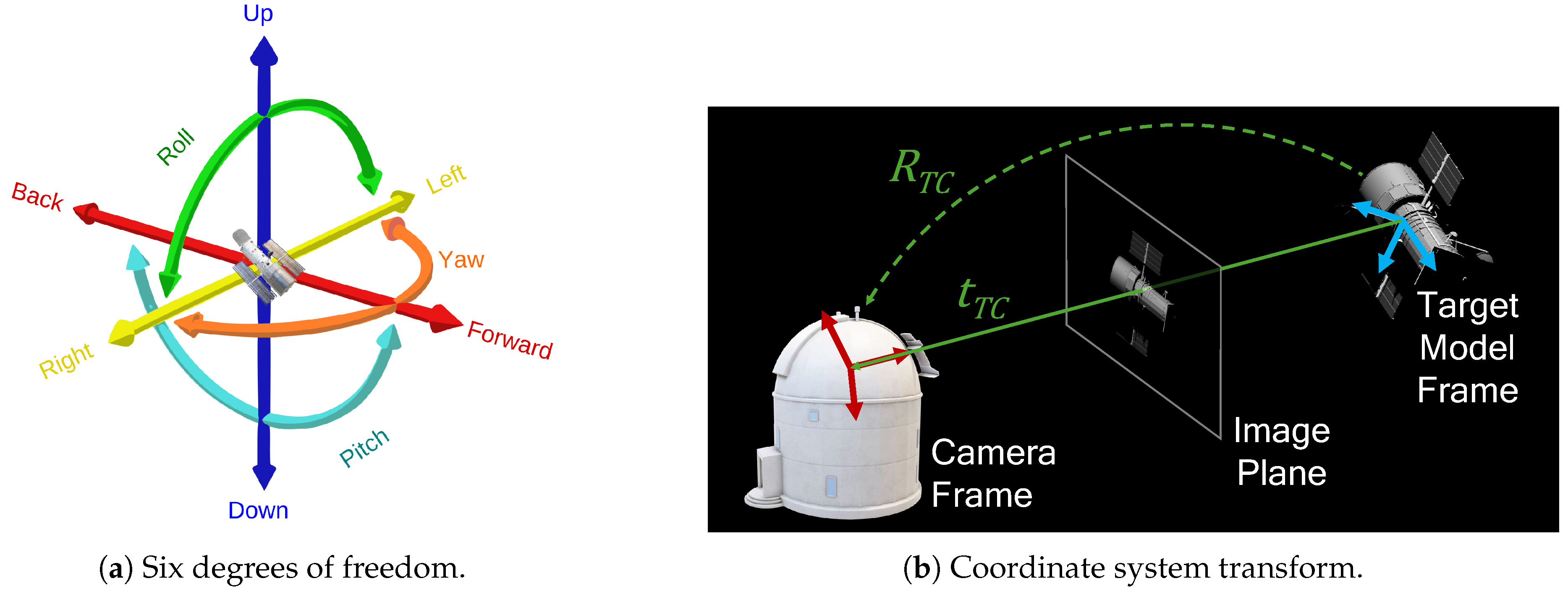
Figure 2.
A pristine render of a hstHST Computer-Aided Design (CAD) model is used to independently illustrate the visual confusion resulting from partial illumination, 3DOF rotation, 3DOF translation, blur, and noise. While HST’s pose in the top left image is obvious, the combined effects of these transformations result in a much more ambiguous pose in the final image.
Figure 2.
A pristine render of a hstHST Computer-Aided Design (CAD) model is used to independently illustrate the visual confusion resulting from partial illumination, 3DOF rotation, 3DOF translation, blur, and noise. While HST’s pose in the top left image is obvious, the combined effects of these transformations result in a much more ambiguous pose in the final image.
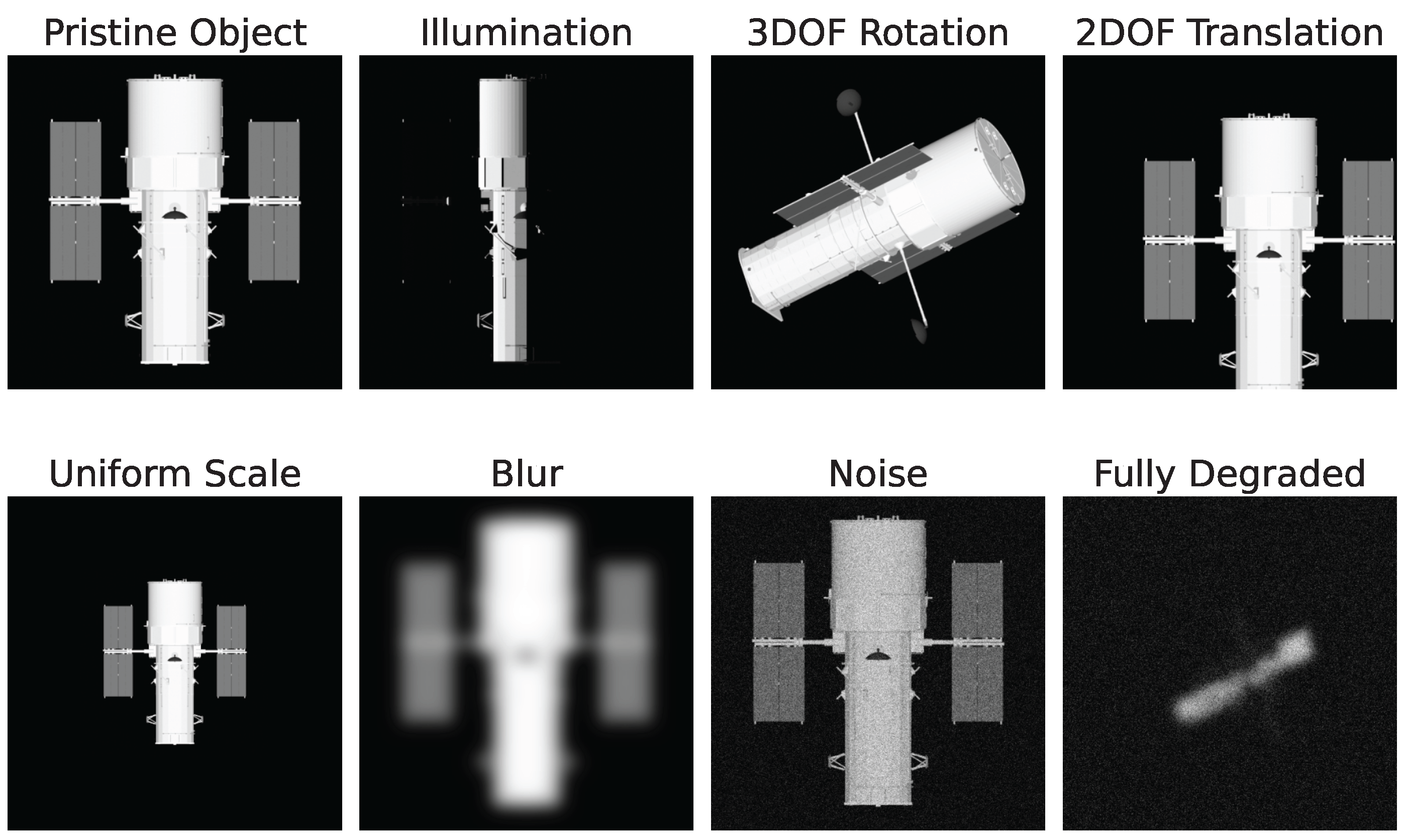
Figure 3.
A 6DOF pose prediction was produced for the underlying grayscale image of the satellite Seasat (SATCAT #10967). The pose prediction was used to align a CAD model, and the model wireframe was overlaid in red on the grayscale image. In this example the previously unobservable position of the unilluminated solar arrays becomes apparent to the viewer.
Figure 3.
A 6DOF pose prediction was produced for the underlying grayscale image of the satellite Seasat (SATCAT #10967). The pose prediction was used to align a CAD model, and the model wireframe was overlaid in red on the grayscale image. In this example the previously unobservable position of the unilluminated solar arrays becomes apparent to the viewer.
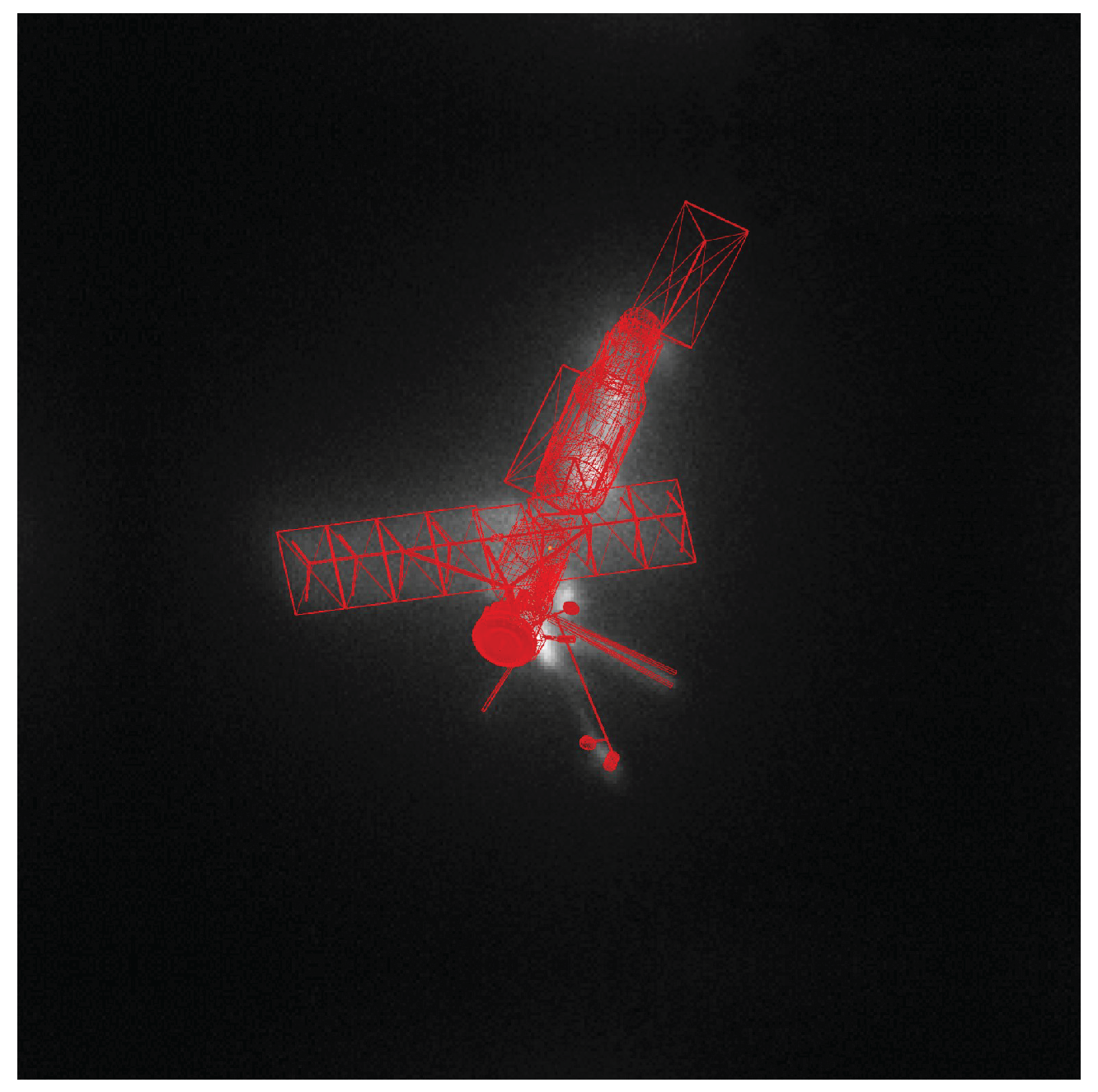
Figure 4.
Solar azimuth and elevation angles (a) and target azimuth and elevation angles (b) for a specified ground site. Solar positions are displayed using a scatter plot, while target positions are displayed as a heatmap with purple indicating zero point density and red indicating maximum.
Figure 4.
Solar azimuth and elevation angles (a) and target azimuth and elevation angles (b) for a specified ground site. Solar positions are displayed using a scatter plot, while target positions are displayed as a heatmap with purple indicating zero point density and red indicating maximum.
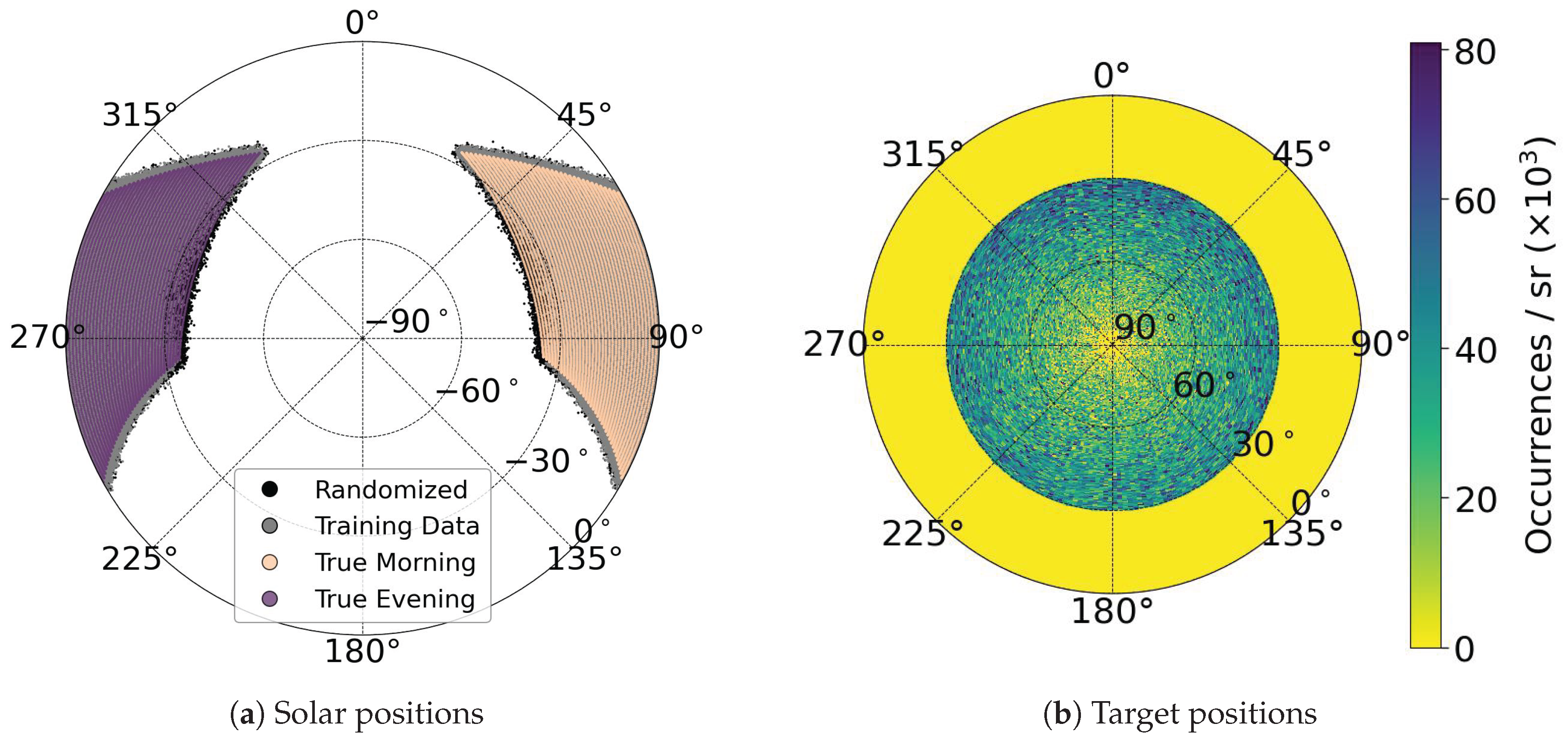
Figure 5.
Histograms of training set quaternion elements (, , , ). Quaternions were uniformly sampled over [23]. Note that uniform sampling in does not produce uniform distributions in quaternion element space.
Figure 5.
Histograms of training set quaternion elements (, , , ). Quaternions were uniformly sampled over [23]. Note that uniform sampling in does not produce uniform distributions in quaternion element space.
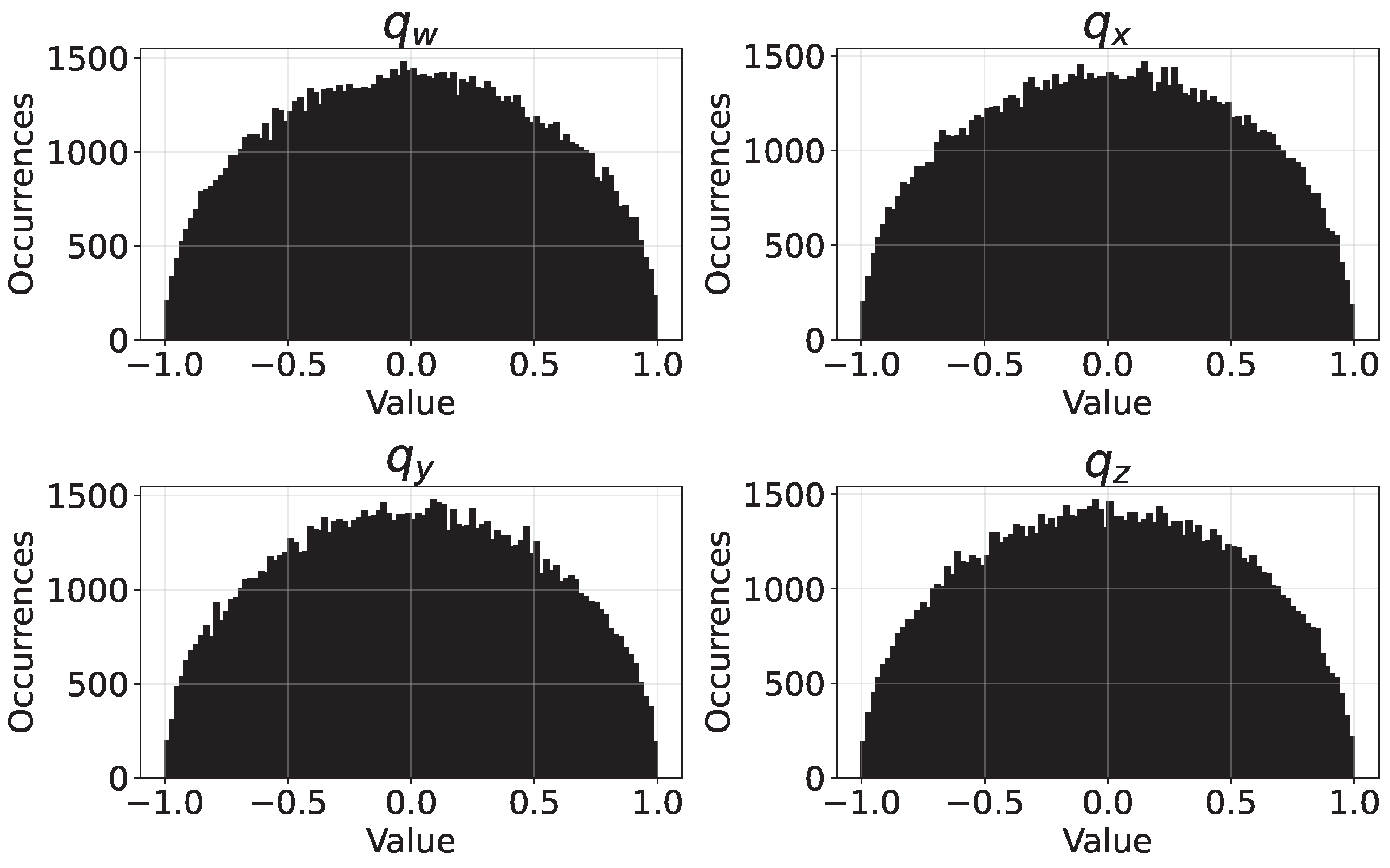
Figure 6.
Image-plane translation offsets for HST training data shown in both pixel coordinates (left) and meters (right). The distributions are largely uniform until approaching the edges of the FOV where uniformity is reduced to meet the constraint of maintaining the full object within the FOV.
Figure 6.
Image-plane translation offsets for HST training data shown in both pixel coordinates (left) and meters (right). The distributions are largely uniform until approaching the edges of the FOV where uniformity is reduced to meet the constraint of maintaining the full object within the FOV.
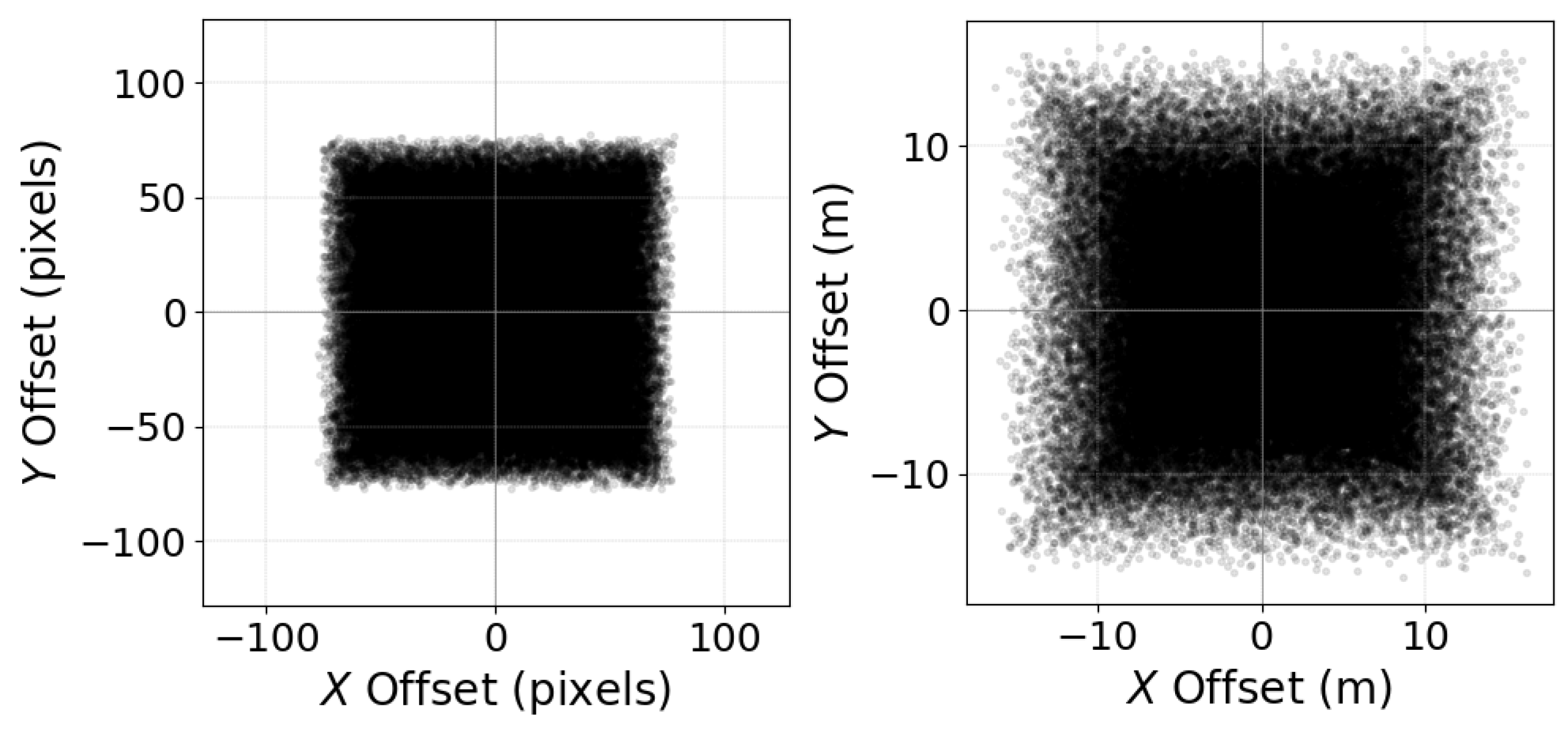
Figure 8.
The ground truth Z components of 3D point maps are visualized using a colormap with partial transparency, overlaid on their corresponding grayscale RoI-cropped synthetic images, showing dense pixelwise 2D↔3D correspondences. These data were generated for coupled pipeline training, where the RoI crop algorithm relied on localizations predicted by the Coarse Localizer. As a result, inaccuracies are evident in the crops.
Figure 8.
The ground truth Z components of 3D point maps are visualized using a colormap with partial transparency, overlaid on their corresponding grayscale RoI-cropped synthetic images, showing dense pixelwise 2D↔3D correspondences. These data were generated for coupled pipeline training, where the RoI crop algorithm relied on localizations predicted by the Coarse Localizer. As a result, inaccuracies are evident in the crops.
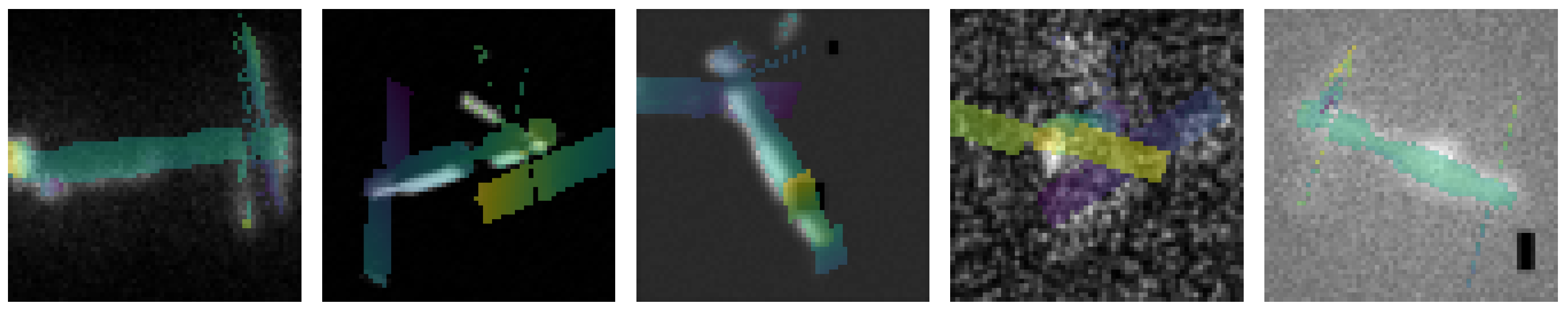
Figure 9.
A 3D visualization of the Seasat point cloud (created by aligning and combining all ) after application of farthest point sampling to segment the geometry and create .
Figure 9.
A 3D visualization of the Seasat point cloud (created by aligning and combining all ) after application of farthest point sampling to segment the geometry and create .
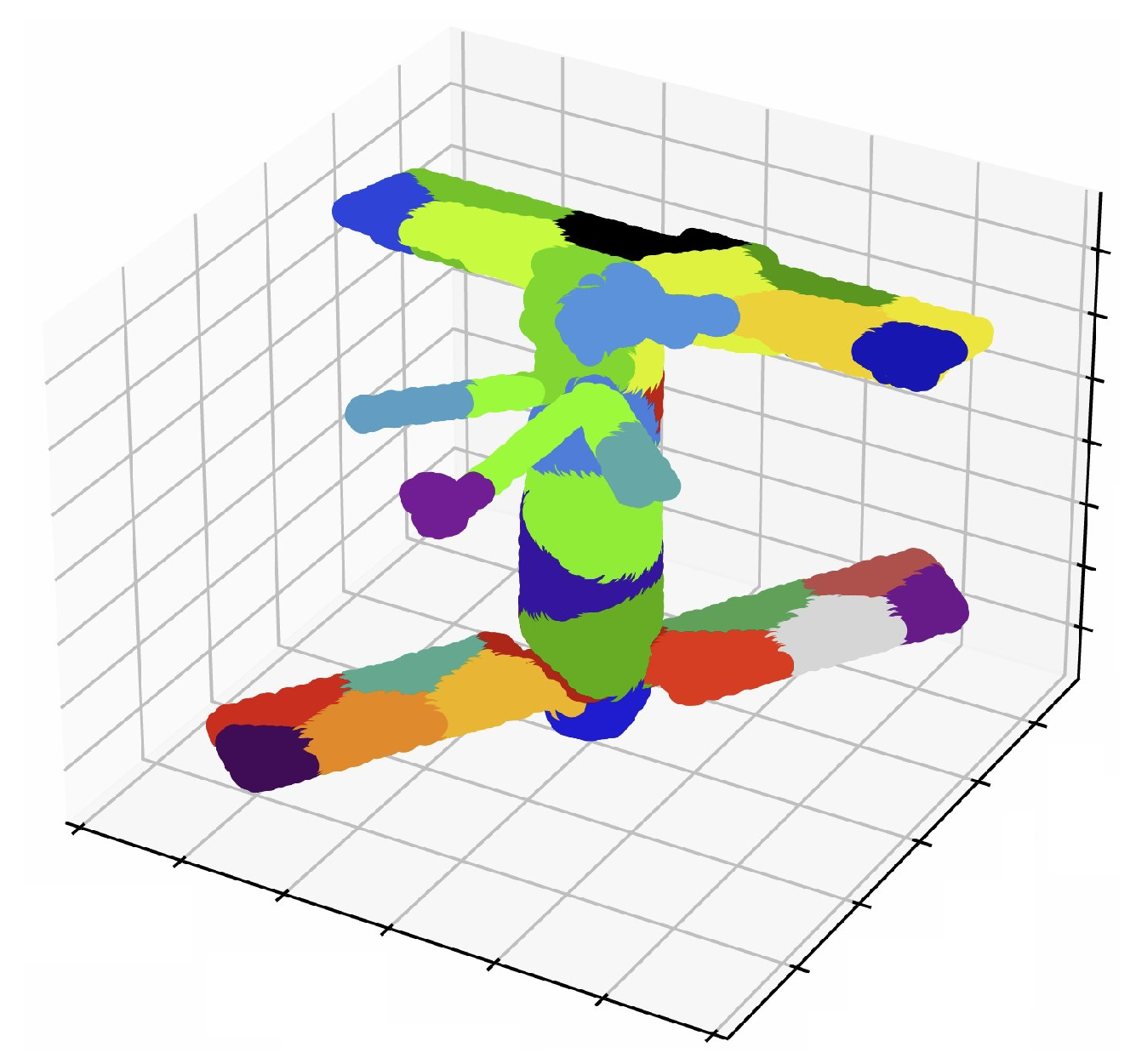
Figure 10.
The first row shows the input RoI cropped test images. The second row displays the corresponding ground truth , where each pixel is assigned one of 33 semantic classes (class 0 for the background in black and 32 object-specific classes in distinct colors). These semantic classes provide a crucial intermediate representation, simplifying the downstream task of regressing the 6DOF pose by first requiring the network to solve the simpler problem of classifying which satellite region each pixel belongs to. The third row illustrates the maps predicted by the U-Net. The U-Net produces per-pixel 33-dimensional vectors via a softmax activation function in the final layer. Each element in the vector represents a softmax-normalized score for one of the 33 classes, indicating the model’s relative confidence for that class. For visualization, these vectors were reduced to their maximum-valued class (the over the 33 classes), and each class was assigned a unique color.
Figure 10.
The first row shows the input RoI cropped test images. The second row displays the corresponding ground truth , where each pixel is assigned one of 33 semantic classes (class 0 for the background in black and 32 object-specific classes in distinct colors). These semantic classes provide a crucial intermediate representation, simplifying the downstream task of regressing the 6DOF pose by first requiring the network to solve the simpler problem of classifying which satellite region each pixel belongs to. The third row illustrates the maps predicted by the U-Net. The U-Net produces per-pixel 33-dimensional vectors via a softmax activation function in the final layer. Each element in the vector represents a softmax-normalized score for one of the 33 classes, indicating the model’s relative confidence for that class. For visualization, these vectors were reduced to their maximum-valued class (the over the 33 classes), and each class was assigned a unique color.
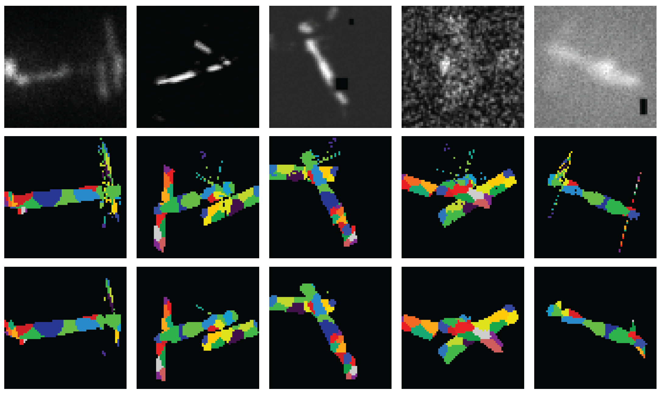
Figure 11.
Ten HST renders showing randomized material properties, illumination strength and diffuse/specular balance, and mliMLI surface texture. Camera parameters, object pose, and illumination direction are held constant for display purposes.
Figure 11.
Ten HST renders showing randomized material properties, illumination strength and diffuse/specular balance, and mliMLI surface texture. Camera parameters, object pose, and illumination direction are held constant for display purposes.
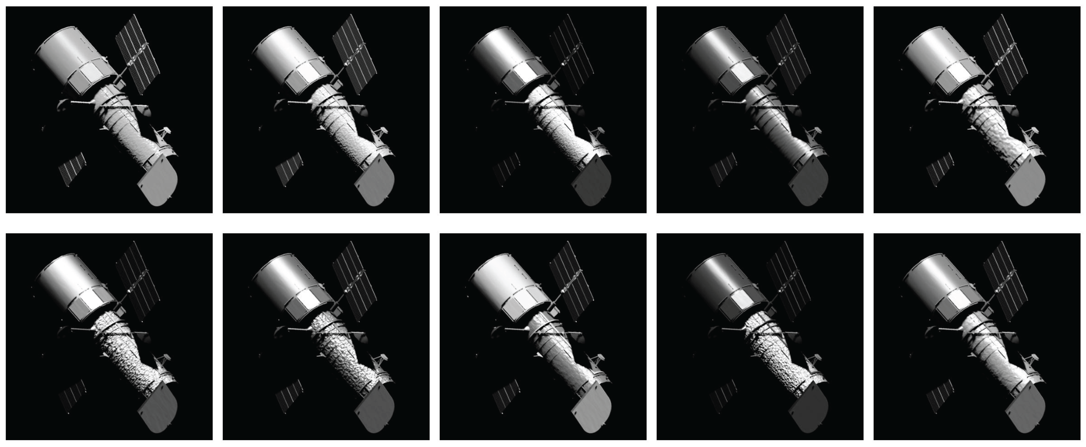
Figure 12.
Five pristine test image renders produced with Blender (top five) and dirsigDIRSIG (bottom five). Despite identical CAD geometry, satellite pose, and illumination directions, the renders appear noticeably different due to DIRSIG’s more advanced simulation pipeline and intentionally distinct material properties designed to stress-test the model’s generalization capability. Renders are displayed with an individual linear min-max stretch.
Figure 12.
Five pristine test image renders produced with Blender (top five) and dirsigDIRSIG (bottom five). Despite identical CAD geometry, satellite pose, and illumination directions, the renders appear noticeably different due to DIRSIG’s more advanced simulation pipeline and intentionally distinct material properties designed to stress-test the model’s generalization capability. Renders are displayed with an individual linear min-max stretch.
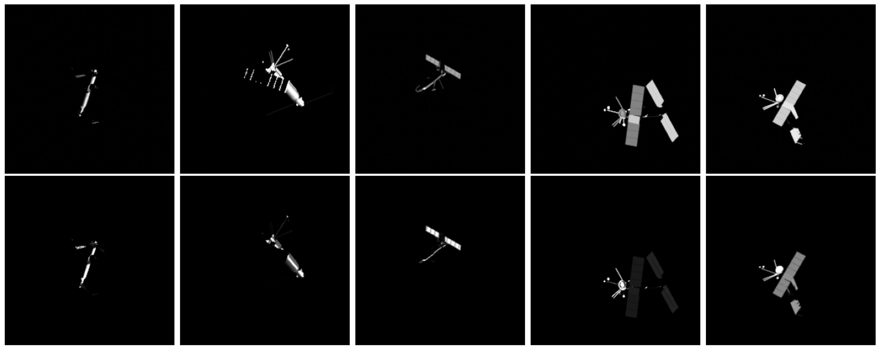
Figure 13.
A psfPSF simulated using hcipyHCIPy, displayed in scale at left and linear scale at right. Complex structure is visible in the PSF. This method is capable of producing highly complex and realistic PSFs.
Figure 13.
A psfPSF simulated using hcipyHCIPy, displayed in scale at left and linear scale at right. Complex structure is visible in the PSF. This method is capable of producing highly complex and realistic PSFs.
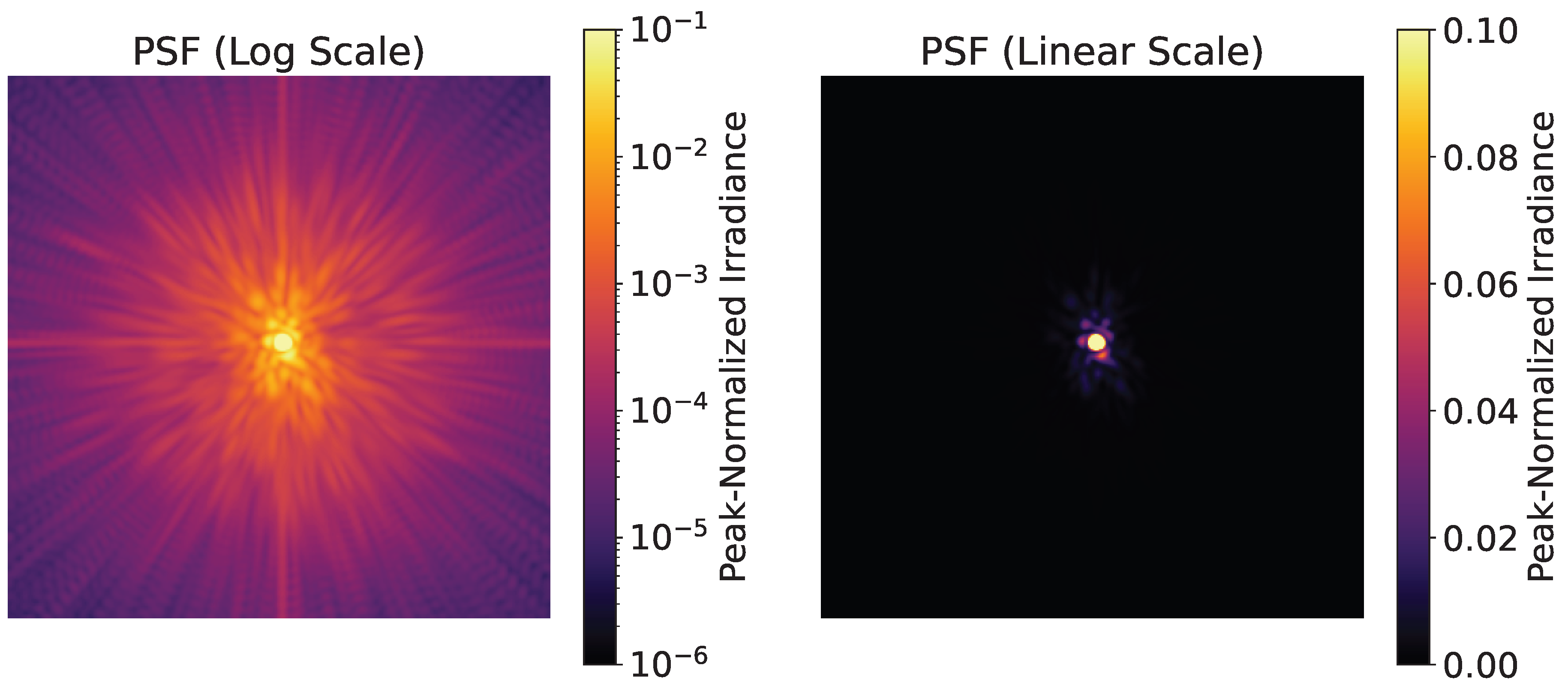
Figure 15.
The first 50 lfidLFID test images from the augmented 6DOF Seasat dataset after the RoI crop and resize algorithm has been applied using the predicted bounding box and object center coordinates.
Figure 15.
The first 50 lfidLFID test images from the augmented 6DOF Seasat dataset after the RoI crop and resize algorithm has been applied using the predicted bounding box and object center coordinates.
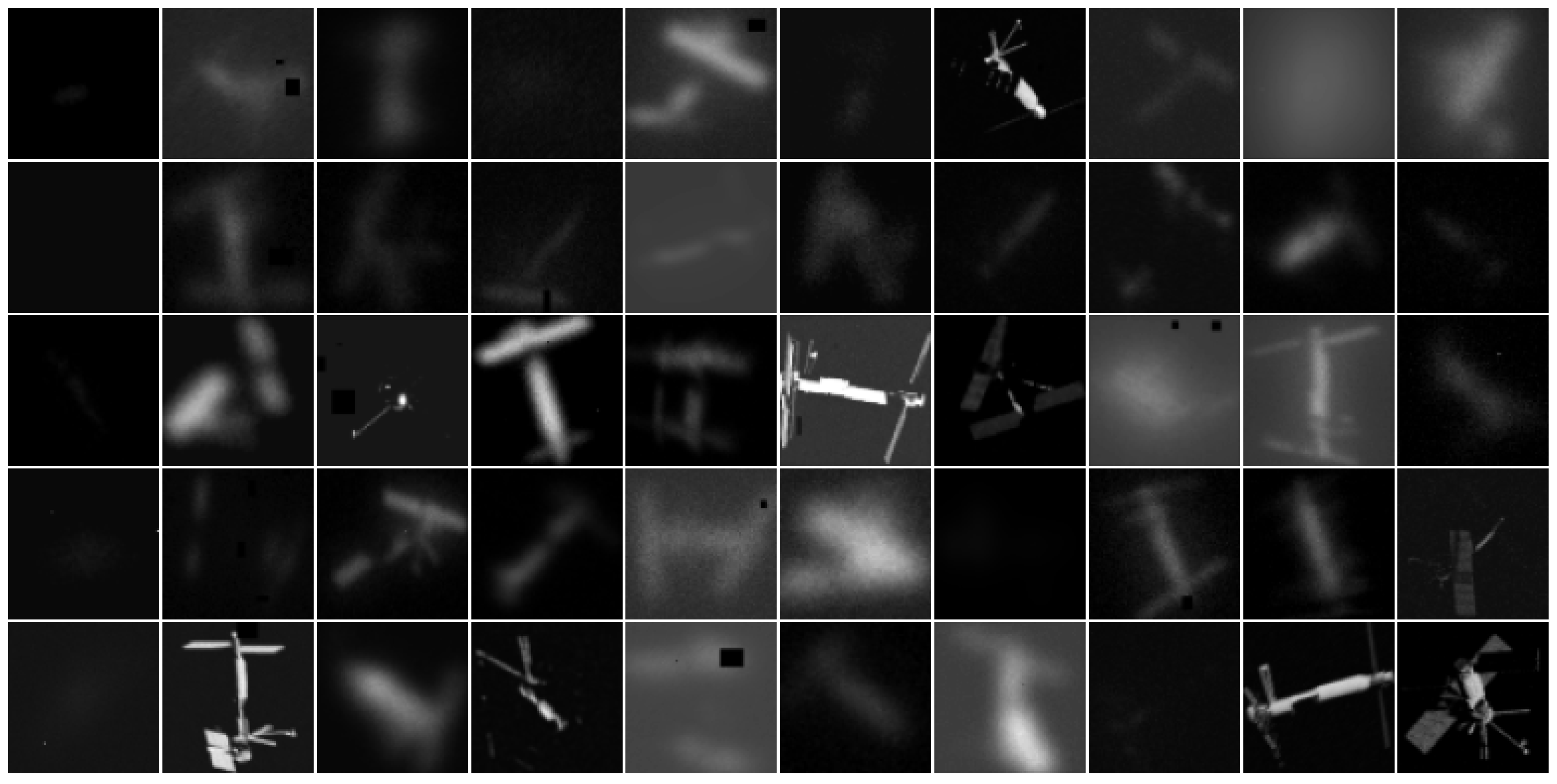
Figure 17.
Training and validation loss as a function of epoch (left), mean LFID validation rotation error in degrees (center), and mean LFID validation two-axis angular translation error in µrad (right) during Stage 4 of PoseNet training. Validation metrics improve rapidly during the first five epochs. Weights were checkpointed based on the best validation loss, and training terminated early (prior to 50 epochs) using a patience of 10 epochs without validation loss improvement.
Figure 17.
Training and validation loss as a function of epoch (left), mean LFID validation rotation error in degrees (center), and mean LFID validation two-axis angular translation error in µrad (right) during Stage 4 of PoseNet training. Validation metrics improve rapidly during the first five epochs. Weights were checkpointed based on the best validation loss, and training terminated early (prior to 50 epochs) using a patience of 10 epochs without validation loss improvement.
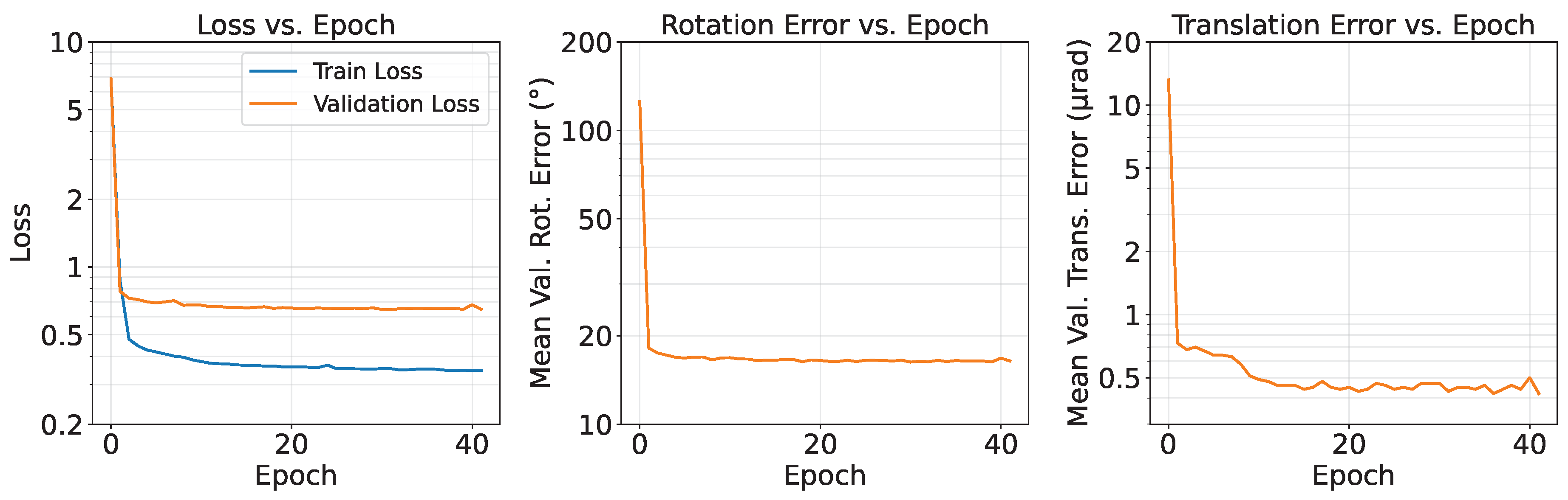
Figure 19.
Comparison of decoupled (blue) and coupled (orange) model performance. The percentage change from decoupled to coupled is shown in black above each of the 12 metrics. The greatest impact was to the 90th percentile rotation error, with a 29% decrease. Performance improved for 11 of 12 metrics, with a 2% increase in 10th percentile range error.
Figure 19.
Comparison of decoupled (blue) and coupled (orange) model performance. The percentage change from decoupled to coupled is shown in black above each of the 12 metrics. The greatest impact was to the 90th percentile rotation error, with a 29% decrease. Performance improved for 11 of 12 metrics, with a 2% increase in 10th percentile range error.
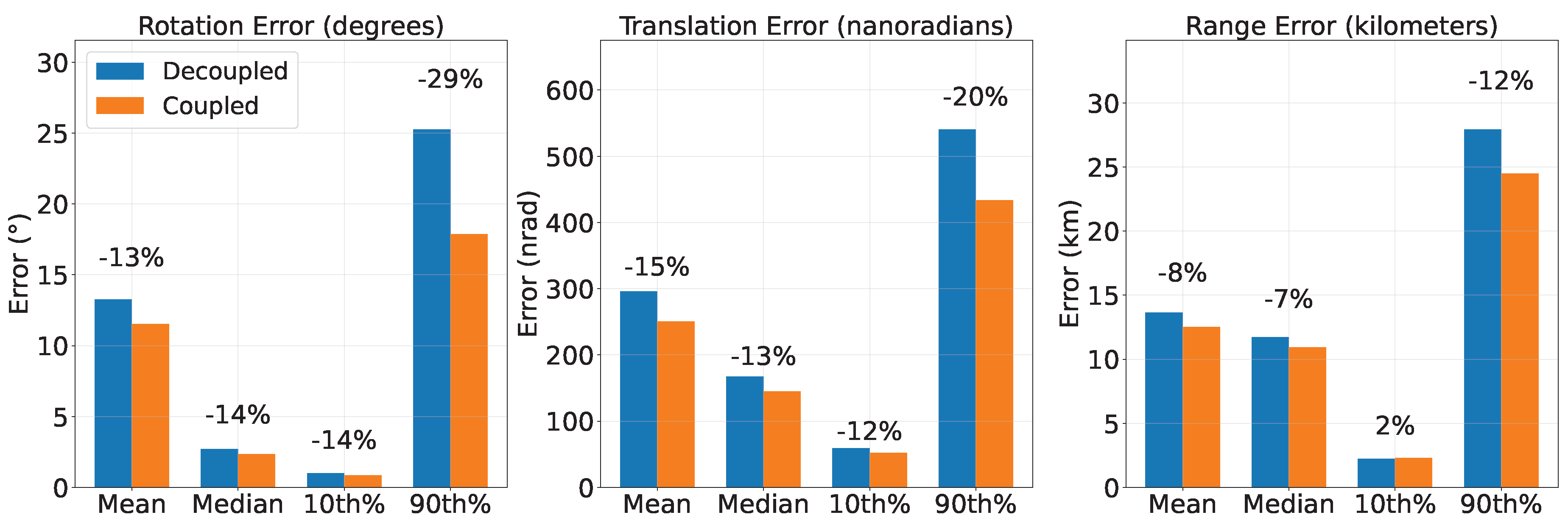
Figure 20.
Pose predictions (red wireframes) overlaid on real Seasat images from SDA AO systems; approximate rotation errors shown at upper left of each panel.
Figure 20.
Pose predictions (red wireframes) overlaid on real Seasat images from SDA AO systems; approximate rotation errors shown at upper left of each panel.
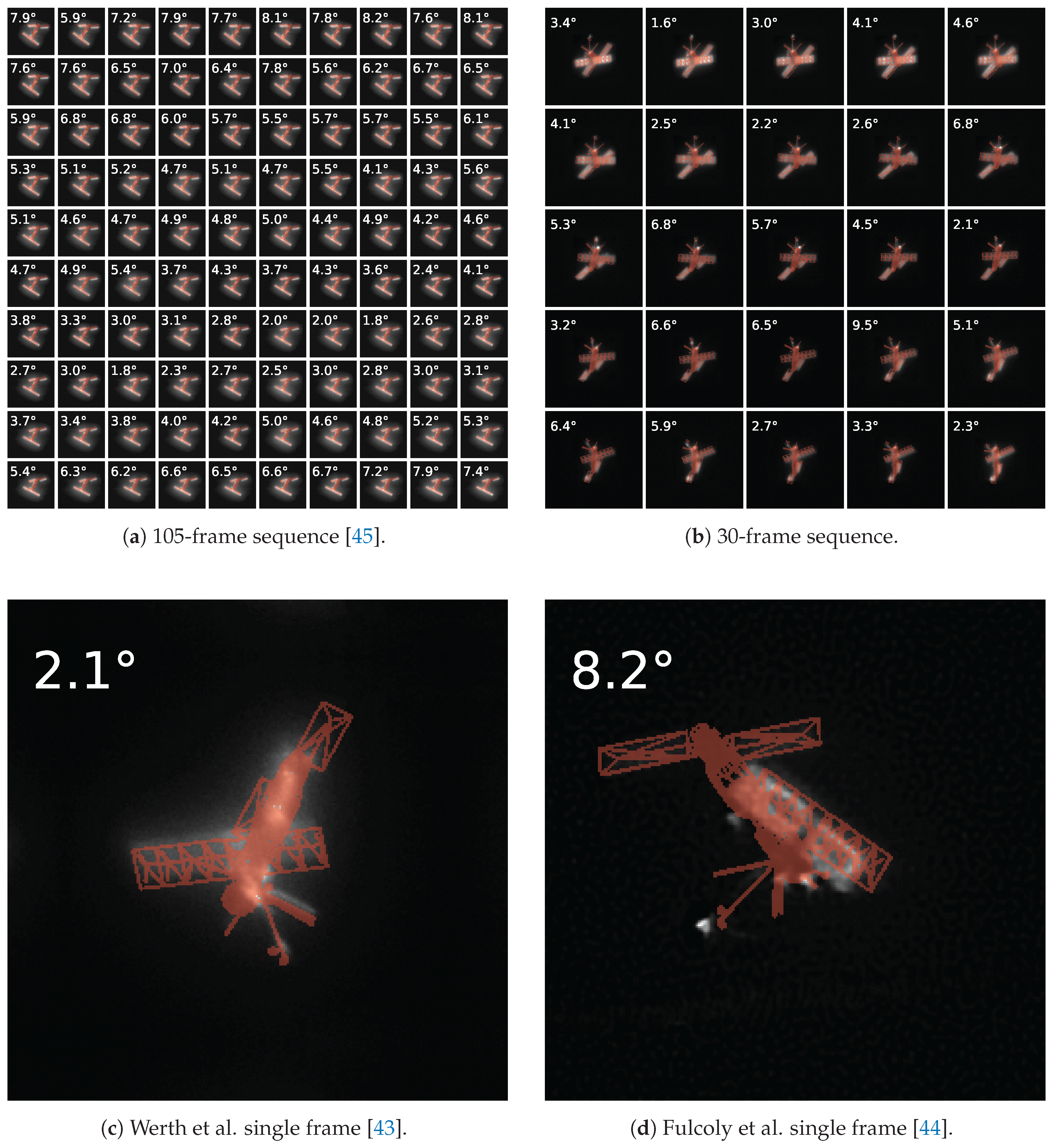
Figure 21.
Red wireframe overlays on a grayscale test image showing notional pose estimates, evaluated left to right using the Satellite Pose Alignment Rating Scale (SPARS): (SPARS-1) catastrophic failure, no silhouette overlap; (SPARS-2) limited success, partial overlap but major misalignment; (SPARS-3) moderate success, good overlap with minor but noticeable errors; (SPARS-4) high confidence match, excellent alignment with only subtle discrepancies; and (SPARS-5) ground truth equivalent, indistinguishable from true pose, even to a trained analyst. The SPARS category is annotated at the upper right of each panel.
Figure 21.
Red wireframe overlays on a grayscale test image showing notional pose estimates, evaluated left to right using the Satellite Pose Alignment Rating Scale (SPARS): (SPARS-1) catastrophic failure, no silhouette overlap; (SPARS-2) limited success, partial overlap but major misalignment; (SPARS-3) moderate success, good overlap with minor but noticeable errors; (SPARS-4) high confidence match, excellent alignment with only subtle discrepancies; and (SPARS-5) ground truth equivalent, indistinguishable from true pose, even to a trained analyst. The SPARS category is annotated at the upper right of each panel.

Figure 22.
Histogram of SPARS evaluation categories for 250 real Seasat images scored by AFRL. Bars are stacked by target elevation <30° vs. ≥30° (model trained only for ≥30°).
Figure 22.
Histogram of SPARS evaluation categories for 250 real Seasat images scored by AFRL. Bars are stacked by target elevation <30° vs. ≥30° (model trained only for ≥30°).
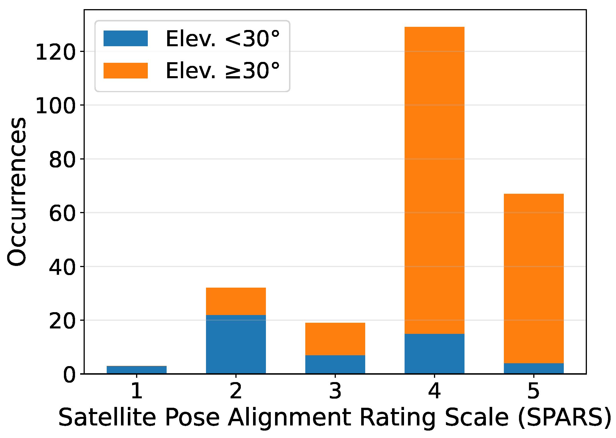
Figure 23.
HST pose overlay for the published frame in [46]; predicted 7DOF pose (including solar array rotation) shown as a red wireframe overlay; body rotation error in degrees at upper left.
Figure 23.
HST pose overlay for the published frame in [46]; predicted 7DOF pose (including solar array rotation) shown as a red wireframe overlay; body rotation error in degrees at upper left.
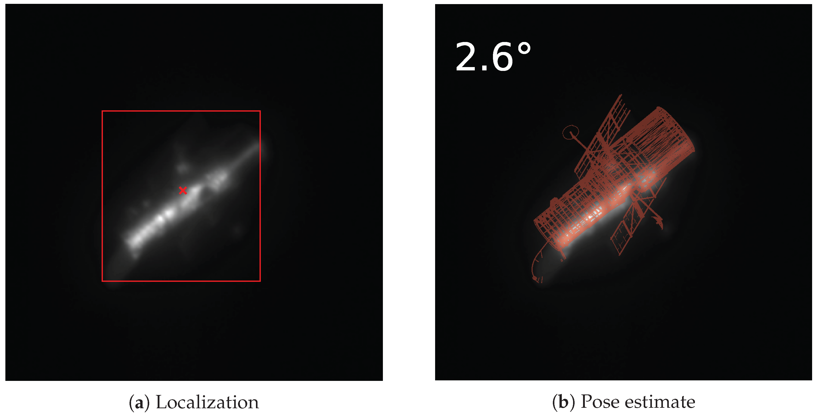
Figure 24.
Per-frame pose errors across 249 real HST frames. Top: body rotation error (deg). Bottom: image-plane translation error (cm). Raw (blue) vs. Kalman-filtered (red).
Figure 24.
Per-frame pose errors across 249 real HST frames. Top: body rotation error (deg). Bottom: image-plane translation error (cm). Raw (blue) vs. Kalman-filtered (red).
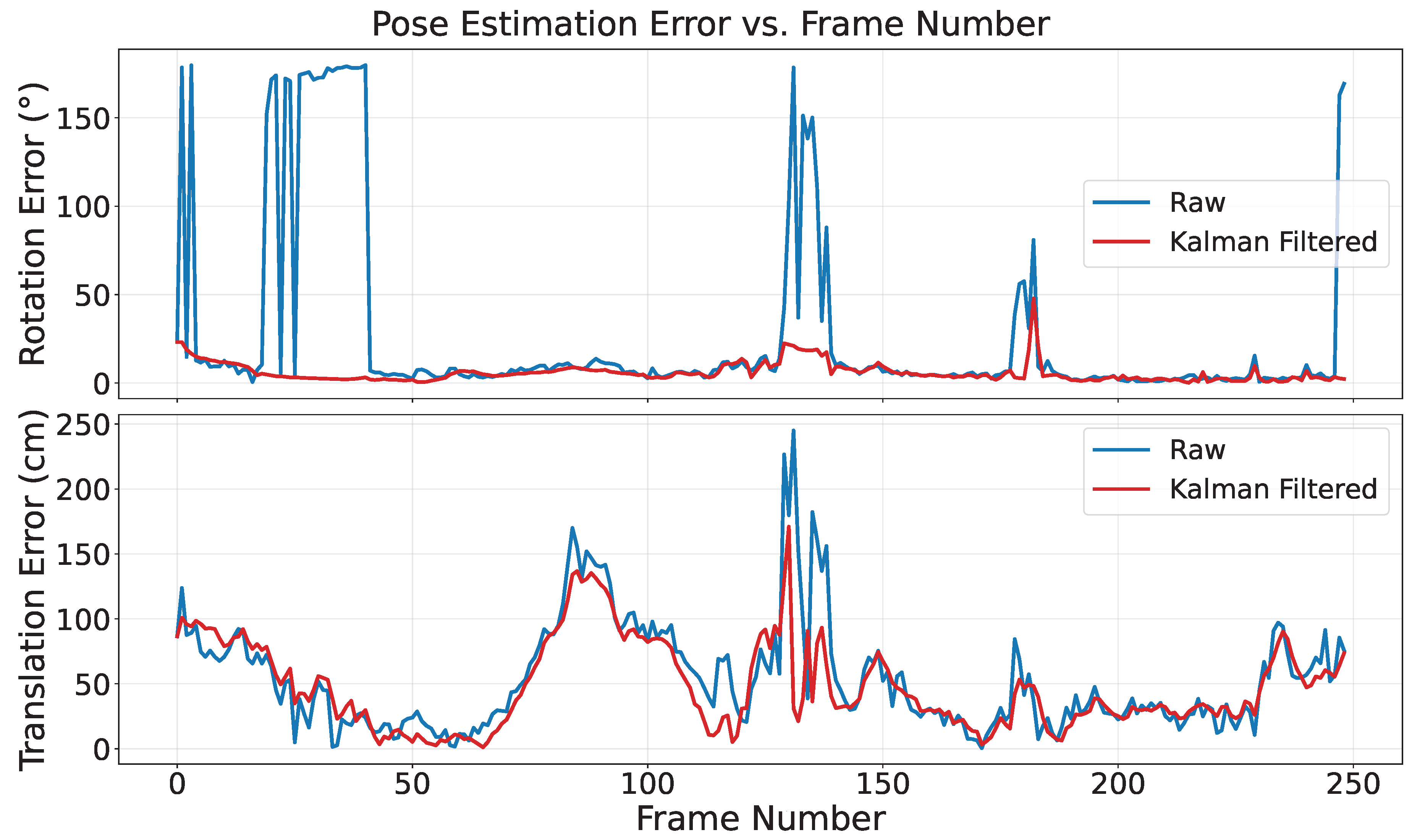
Figure 25.
Per-frame solar-array rotation error for the 249-frame HST pass. Raw (blue) exhibits 180° ambiguity; symmetry-adjusted (orange) and Kalman-filtered (red) curves show substantial reduction.
Figure 25.
Per-frame solar-array rotation error for the 249-frame HST pass. Raw (blue) exhibits 180° ambiguity; symmetry-adjusted (orange) and Kalman-filtered (red) curves show substantial reduction.
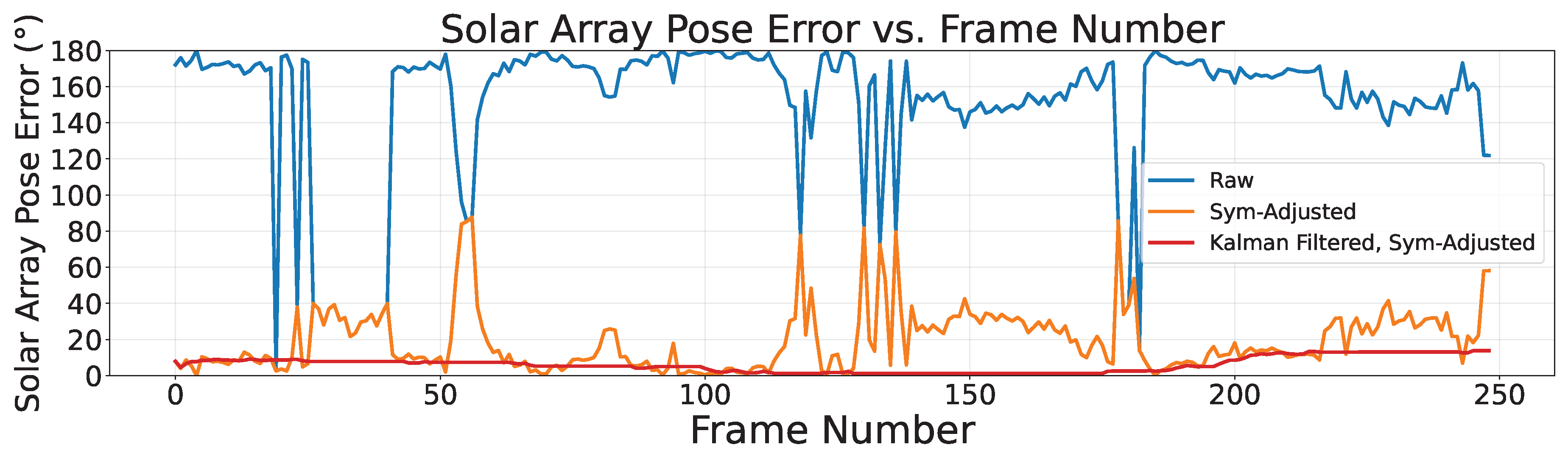
Figure 26.
Seasat errors were averaged over each atmosphere and plotted as a function of mean aoiqAO-IQ score for the test images resulting from that atmosphere. An exponential decay function was fit to the data, demonstrating high coefficients of determination.
Figure 26.
Seasat errors were averaged over each atmosphere and plotted as a function of mean aoiqAO-IQ score for the test images resulting from that atmosphere. An exponential decay function was fit to the data, demonstrating high coefficients of determination.
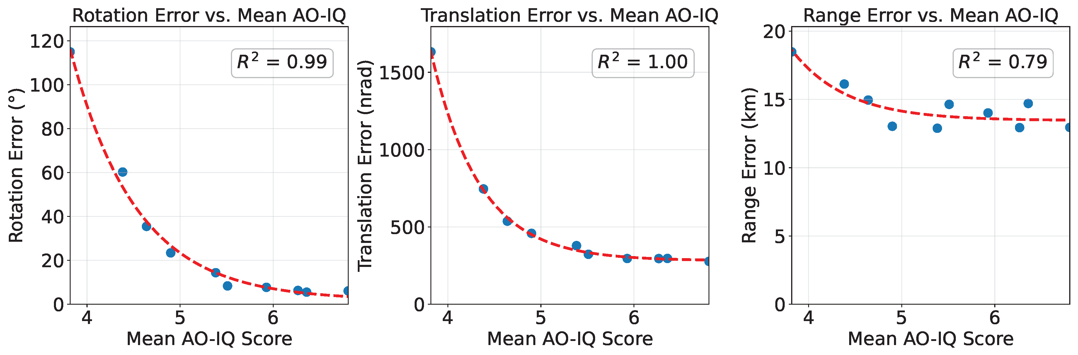
Figure 30.
(a) Two views of opposing sides of the HST satellite CAD model. As with ARGOS, the silhouettes are highly similar. (b) Histogram of HST rotation errors shows clustering near 180°, indicating apparent symmetry as a key error source, albeit less dominant than for ARGOS (see Figure 28).
Figure 30.
(a) Two views of opposing sides of the HST satellite CAD model. As with ARGOS, the silhouettes are highly similar. (b) Histogram of HST rotation errors shows clustering near 180°, indicating apparent symmetry as a key error source, albeit less dominant than for ARGOS (see Figure 28).
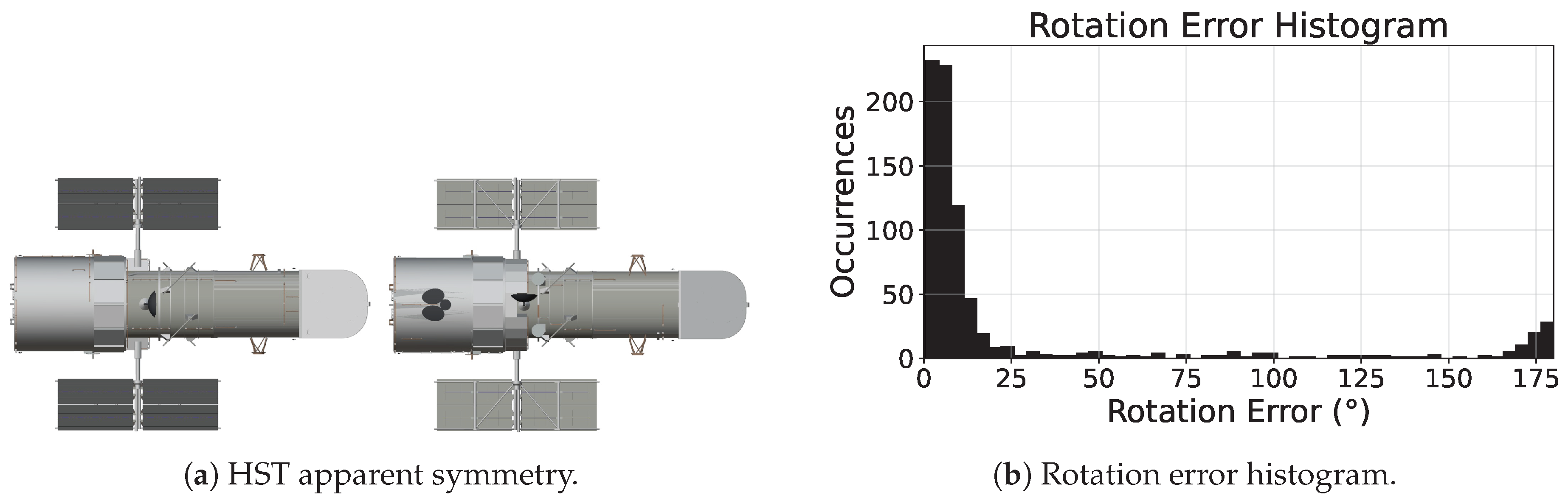
Figure 33.
The single-material 100-triangle Seasat CAD model, composed of a cylinder, triangular prism, and two rectangular prisms is at left. The 15-material 729-triangle Seasat CAD model created by applying Blender’s decimate modifier to the original model is at center. The 17-material 34k-triangle full-fidelity Seasat CAD model is at right.
Figure 33.
The single-material 100-triangle Seasat CAD model, composed of a cylinder, triangular prism, and two rectangular prisms is at left. The 15-material 729-triangle Seasat CAD model created by applying Blender’s decimate modifier to the original model is at center. The 17-material 34k-triangle full-fidelity Seasat CAD model is at right.
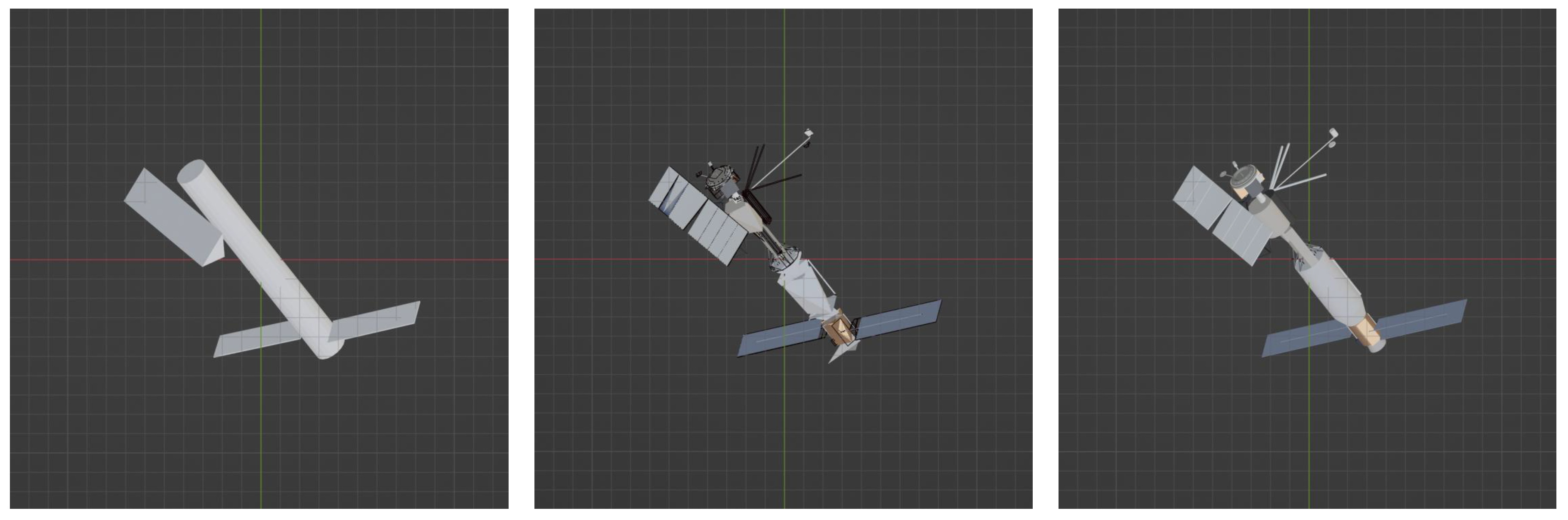
Figure 34.
Cumulative fractional distributions of rotation (a) and two-axis apparent angular translation (b) errors comparing performance of a human labeler to the computer vision pose model. As shown, the pose model significantly outperformed the human expert.
Figure 34.
Cumulative fractional distributions of rotation (a) and two-axis apparent angular translation (b) errors comparing performance of a human labeler to the computer vision pose model. As shown, the pose model significantly outperformed the human expert.
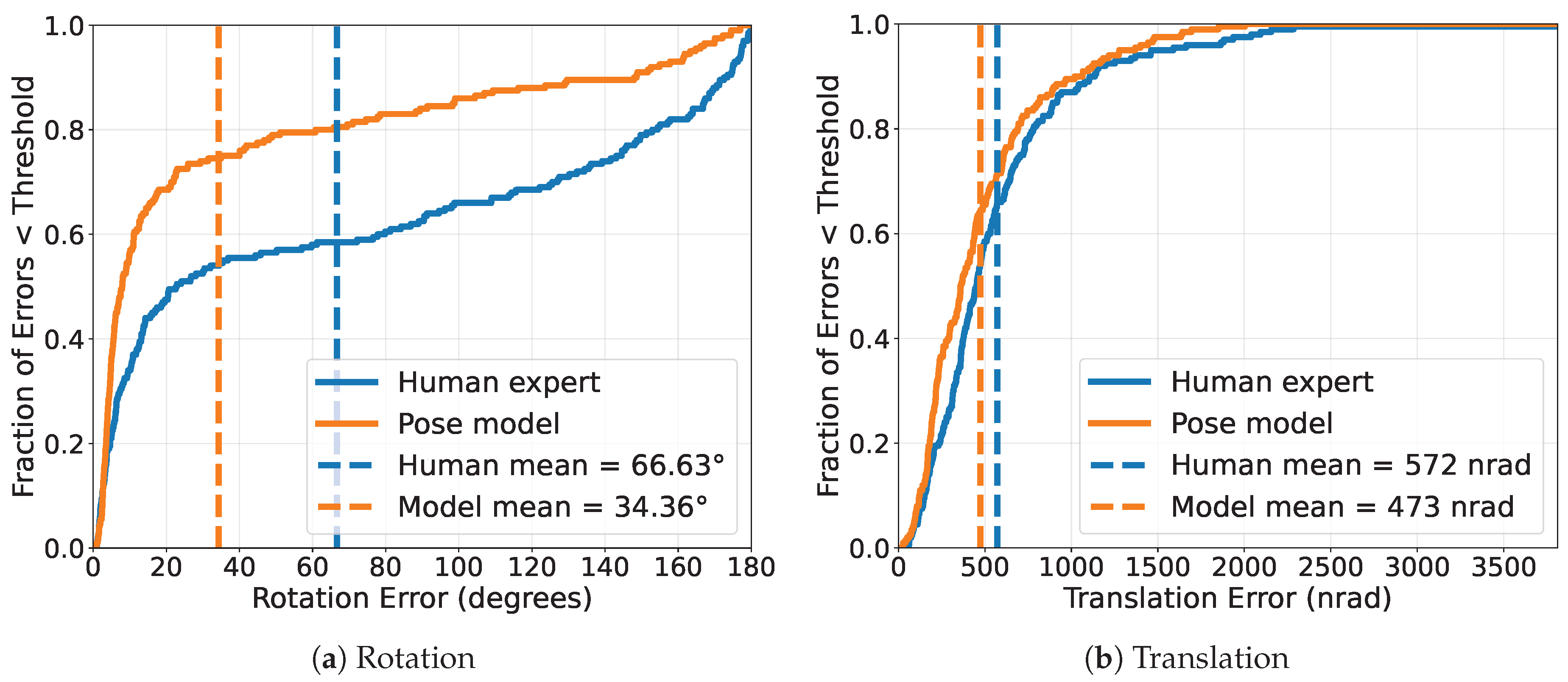
Figure 35.
The top row shows ten simulated test images, the second row shows corresponding ground truth depth maps, the third row shows predicted depth outputs from a custom model trained on synthetic sdaSDA imagery, and the final row shows predicted depth outputs from Depth Anything V2 [54]. All depth maps use the turbo colormap (red = near, purple = far) with per-image min-max normalization (linear contrast stretching).
Figure 35.
The top row shows ten simulated test images, the second row shows corresponding ground truth depth maps, the third row shows predicted depth outputs from a custom model trained on synthetic sdaSDA imagery, and the final row shows predicted depth outputs from Depth Anything V2 [54]. All depth maps use the turbo colormap (red = near, purple = far) with per-image min-max normalization (linear contrast stretching).
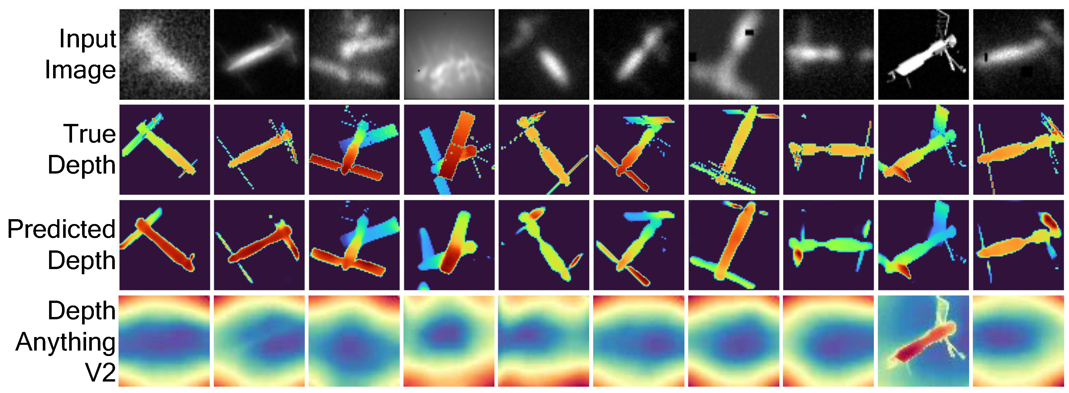
Table 1.
Rotation and translation error statistics for all 137 real Seasat test images, separated by dataset. The Werth et al. [43] and Fulcoly et al. [44] datasets are individual frames. For the results below all test frames were processed individually, with no Kalman filtering.
| Dataset | Rotation Error (°) | Translation Error (cm) | ||||||
|---|---|---|---|---|---|---|---|---|
| Mean | Median | Min | Max | Mean | Median | Min | Max | |
| 105 Frame Video | 5.2 | 5.1 | 1.8 | 9.2 | 16 | 15 | 2.5 | 35 |
| 30 Frame Video | 4.1 | 3.3 | 1.6 | 9.5 | 36 | 26 | 0.8 | 93 |
| Werth et al. | 2.1 | – | – | – | 59 | – | – | – |
| Fulcoly et al. | 8.2 | – | – | – | 39 | – | – | – |
| All Combined | 5.0 | 4.9 | 1.6 | 9.5 | 21 | 19 | 0.8 | 93 |
| Standard Deviation | 1.9 | – | – | – | 17 | – | – | – |
Table 2.
Qualitative evaluation results for 250 real Seasat test images using the SPARS metric, separated into elevation angles below and above the 30° training cutoff.
Table 2.
Qualitative evaluation results for 250 real Seasat test images using the SPARS metric, separated into elevation angles below and above the 30° training cutoff.
| SPARS Level | All () | Elev. <30° () | Elev. ≥30° () |
|---|---|---|---|
| SPARS-1 (Catastrophic Failure) | 3 (1.2%) | 3 (5.9%) | 0 (0.0%) |
| SPARS-2 (Limited Success) | 32 (12.8%) | 22 (43.1%) | 10 (5.0%) |
| SPARS-3 (Moderate Success) | 19 (7.6%) | 7 (13.7%) | 12 (6.0%) |
| SPARS-4 (High Confidence Match) | 129 (51.6%) | 15 (29.4%) | 114 (57.3%) |
| SPARS-5 (Ground Truth Equiv.) | 67 (26.8%) | 4 (7.8%) | 63 (31.7%) |
| Mean SPARS | 3.90 | 2.90 | 4.16 |
Table 3.
Rotation, translation, and solar array angle error statistics for real HST test imagery. The Bennett et al. [46] image is a single published frame. The 249-frame video dataset was processed independently (no temporal context), with and without Kalman filtering. Solar array angle errors are adjusted for 180° symmetry where noted.
Table 3.
Rotation, translation, and solar array angle error statistics for real HST test imagery. The Bennett et al. [46] image is a single published frame. The 249-frame video dataset was processed independently (no temporal context), with and without Kalman filtering. Solar array angle errors are adjusted for 180° symmetry where noted.
| Dataset | Rotation Error (°) | Translation Error (cm) | Solar Array Error (°) | |||||||
|---|---|---|---|---|---|---|---|---|---|---|
| Mean | Median | Min | Max | Mean | Median | Min | Max | Mean | Max | |
| Bennett et al. | 2.6 | – | – | – | 11 | – | – | – | 8 | – |
| 249 Frame Video (No KF) | 27.1 | 6.4 | 0.6 | 179.8 | 54 | 41 | 1 | 245 | 19 | 88 |
| 249 Frame Video (KF Applied) | 5.9 | 4.3 | 0.2 | 47.8 | 48 | 37 | 1 | 171 | 6 | 14 |
| Standard Deviation | 5.5 | – | – | – | 33 | – | – | – | 4 | – |
Solar array angle errors adjusted for 180° symmetry.
Standard deviation for Kalman-filtered 249-frame video.
Disclaimer/Publisher’s Note: The statements, opinions and data contained in all publications are solely those of the individual author(s) and contributor(s) and not of MDPI and/or the editor(s). MDPI and/or the editor(s) disclaim responsibility for any injury to people or property resulting from any ideas, methods, instructions or products referred to in the content. |
© 2026 by the authors. Licensee MDPI, Basel, Switzerland. This article is an open access article distributed under the terms and conditions of the Creative Commons Attribution (CC BY) license (http://creativecommons.org/licenses/by/4.0/).
Copyright: This open access article is published under a Creative Commons CC BY 4.0 license, which permit the free download, distribution, and reuse, provided that the author and preprint are cited in any reuse.


