
Submitted:
15 July 2026
Posted:
16 July 2026
You are already at the latest version
Abstract
Experimental studies of the “Turbine Last Stage – Exit Diffuser” system were carried out on the ET4 test bench of the Turbine Engineering Laboratory of the St. Petersburg Polytechnic University. The diffuser model design allowed for the effect of anti-surge bypass of compressor air into the diffuser on its aerodynamic characteristics to be taken into account. The flow structure in the flow section of the model compartment was studied by traversing 3D flow in control sections using five-channel pneumometric probes. Based on the measurement results, an analysis of the integral characteristics and the three-dimensional flow structure in the exhaust manifold was performed. The studies were conducted in the range from 110% of the nominal load to the idle mode of the last stage. Numerical modeling was performed using ANSYS CFX 2023 R1. RANS equations were closed using the SST turbulence model. Comparison of experimental results and numerical modeling showed good agreement in the integral characteristics within a range of up to 50% of the nominal load. At extreme partial load conditions, significant flow pulsations were observed in the annular section of the diffuser, requiring more detailed transient measurements. Based on the study’s results, requirements were formulated for modifying the experimental setup and measurement system to enable pressure pulsation studies under varying load conditions down to the gas turbine’s idle mode.
Keywords:
gas turbine
; extreme partial operating modes
; idle speed
; experimental bench ET4
; aerodynamics
; pressure pulsation
; ANSYS CFX
1. Introduction
Commissioning and start-up modes of stationary gas turbine units are carried out without external load at idle speed. The ‘idle’ mode is also implemented each time the GTU is started in order to preheat it. Such ‘idle’ modes of GTU operation can last for a fairly long time. At the same time, the flow of the working medium in the turbine changes significantly compared to the nominal mode.
The most significant changes in the flow structure occur in the last stage of the turbine, which can even switch to power absorption modes (ventilation modes). In this case, a complex three-dimensional rearrangement of the outgoing flow occurs [1] (pp.16-25) with very high turbulence at its entry into the diffuser. Since modern stationary GTU designs include power struts for mounting the rear bearing, their flow at ‘idle speed’ occurs at significant angles of attack, which causes periodic or aperiodic pressure pulsations. Experiments have shown that these pulsations also propagate ‘upstream,’ which can lead to resonant vibrations of turbine components [2] (p.324) and disturbances in the combustion chamber.
With the specified flow around the diffuser support struts, the stall phenomena are unsteady and stochastic in nature and the only way to obtain a reliable picture of the flow is to conduct a physical experiment. Such an experiment will be conducted in the facilities of the aerodynamics laboratory I.I Kirilov in St. Petersburg Polytechnic University on the ET4 test bench[3] pp(38,47), but for that, the test bench needs to be modified with 1) the addition of an auxiliary system for additional power to the shaft(APSS-additional power supply system) and 2) the addition of low inertia sensors on the power struts and the diffuser after their positioning has been defined. If all the above is done, the actual experiment can then be implemented. In this paper the preliminary calculations and CFD analysis is done in order to cover the aforementioned topics so as to lay the foundation for the final future experiment, which will in its turn, give us the necessary measurements and results on static pressure pulsation during idling mode of a turbine [4] (pp28-40).
For this reason, it is necessary to study potential pulsation phenomena in the flow section of the gas turbine exhaust system. This study involves:
- simulation of the idle mode of the final stage and the idle mode of the gas turbine;
- determination of the characteristics of pulsation processes in the flow section of the exhaust duct during idle modes;
- determination of the main aerodynamic characteristics of the stage and the “stage–exhaust diffuser” system (the ‘S–D’ system) during GT idle operation.
For experimental studies of the aerodynamics of a turbine exhaust duct under extreme operating conditions, it is advisable to use the ET4 test bench at the Turbine Engineering Laboratory of St. Petersburg Polytechnic University, which is equipped with a model of the Stage-Diffuser ‘S–D’ system of a high-power gas turbine. However, to simulate the gas turbine idling mode in the ‘S–D’ model, additional power must be supplied from an external source to the impeller of the model’s final stage. Only in this case can the gas flow process in the ‘S–D’ model system be simulated during the gas turbine idling mode. Essentially, it is necessary to implement in the model a highly swirled flow behind the final turbine stage with an exit angle α2m < α1m (flow angles a2 and a1 in the middle of the rotor blade and guide vane respectively), which will be accompanied by intense separation phenomena as the flow passes around the power struts in the diffuser.
A theoretical and experimental study of these processes was conducted at the SPbPU Turbine Engineering Laboratory at the request of a major turbine manufacturing company. Ultimately, data were obtained on the aerodynamics of the exhaust duct in the load range from 110% of rated power to gas turbine idling, as well as the distribution of pressure pulsations on the surfaces of the outlet stator/sleeve diffuser during last-stage idling and gas turbine idling. The study of the dynamics of extreme partial operating modes required a significant amount of preliminary work and the development of a unique experimental methodology. First and foremost, this involved determining the amount of additional power required to reach the gas turbine idling mode in the experiment with the ‘S–D’ model and modifying the ET4 test bench. This paper presents the results of computational and experimental studies of the aerodynamics of the ‘S-D’ system over a load range of 0–110% of the rated value, which enabled the modification of the ET4 test bench and the development of a method for measuring pressure pulsations in the outlet duct [5] (p216).
Thus, the main objectives and the set scientific target of the preliminary studies presented in the article are:
- Simulation of the aerodynamics of the ‘S-D’ system in the range from 110% of the rated load to the idle mode of the final stage;
- Validation of the computational flow model in the ‘S-D’ model section;
- Determination of the additional power required to bring the ‘S-D’ model to gas turbine idling;
- Development of a pressure pulsation measurement system and methods for their analysis.
2. Materials and Methods
2.1. Experimental Test Bench ET4 with a Model of the ‘S-D’ System
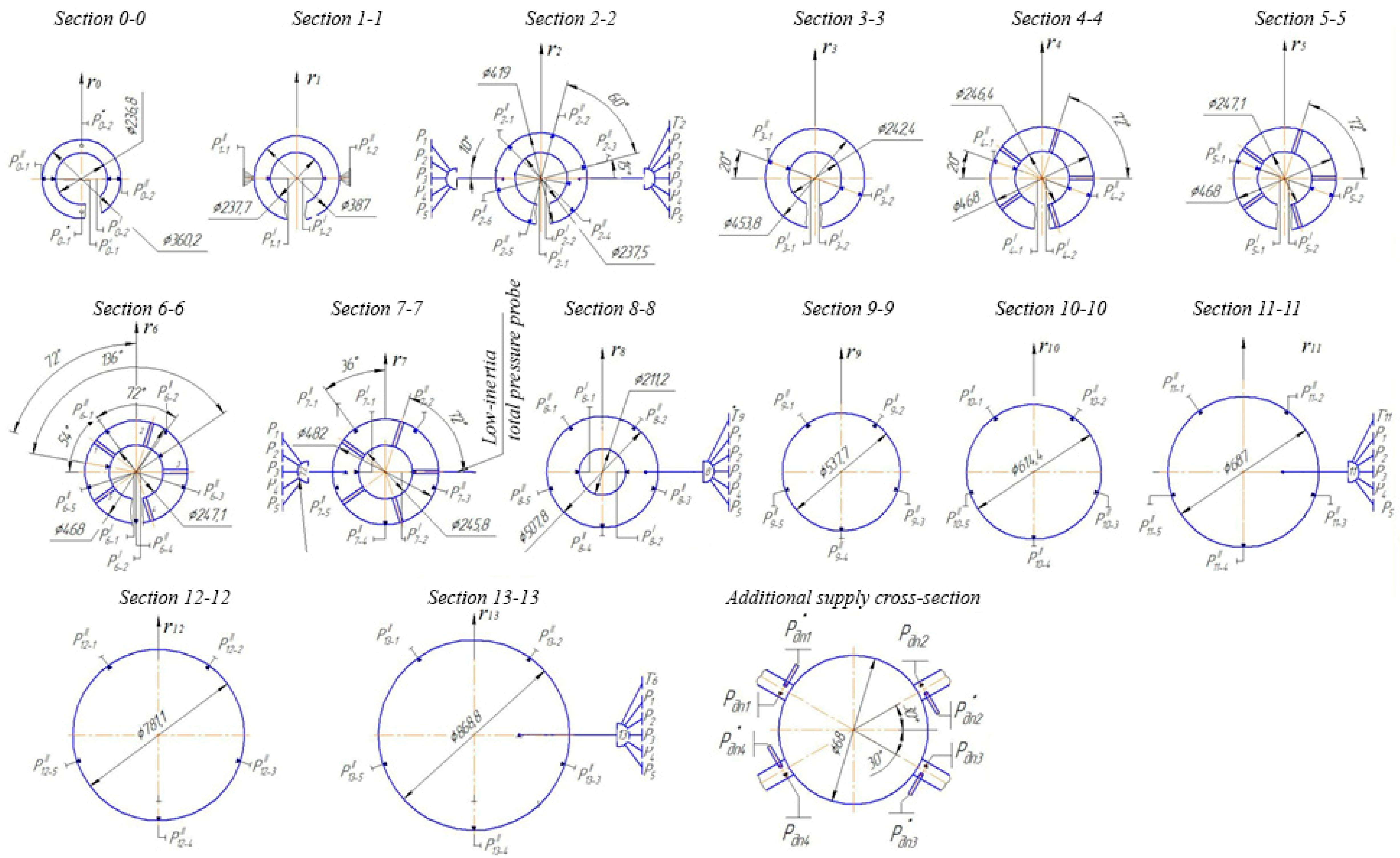
A longitudinal section of the ET4 [6] test bench with the installed model of the ‘S-D’ system is shown in Figure 2.1, and a photograph of the test bench from the side of the hydraulic brake and outlet diffuser is shown in Figure 2.2 and 2.3. The design of the model compartment is such that it simulates the “bypass” of the working fluid around the turbine when simulating extreme partial load conditions. For this purpose, in addition to the main flow entering through the flow-metering nozzle into the equalizing tank and then into the model compartment, an additional air supply is organized in the conical part of the diffuser. Its volume is controlled by a second flow-metering nozzle (the flow-metering nozzle of the ET3 rig). The design of the additional supply is equipped with an additional valve for regulating its flow (Figure 2.4). Flexible plastic pipelines with an internal diameter of Φ68 mm are made of the same length Ltr = 1.5 m, and, consequently, with similar values of air flow resistance in individual supplies. Figure 2.1 shows the control and measuring sections numbered 0–13. Five control sections (2-2, 7-7, 8-8, 11-11, 13-13) are used. In addition, drains for measuring wall pressures are provided along the entire length of the model diffuser, both on the peripheral and on its sleeve/stator surface. In this case, either five drains (from section 6-6 to section 13-13) or two drains (from section 1-1 to section 5-5) are provided along the circumference of the selected section. The exception is section 2-2, which has two drains on the sleeve surface and five drains on the peripheral.
The “Stage-Diffuser” model block is manufactured at a reduced scale of 1:4.566 relative to the actual object. All dimensions of the flow path of the model compartment, including the radial clearances at the root of the guide vane and at the impeller periphery, are precisely matched and scaled to the selected scale. This ensures geometric similarity to the object under study.
Kinematic similarity of the flows is maintained by the equality of three similarity coefficients: the stage’s degree of reactivity, the circulation coefficient (or characteristic number), and the flow coefficient. This equality ensures similarity of the velocity triangles in the full-scale and model stages.
To ensure dynamic similarity between the model and actual flows, it is necessary to maintain the equality of the Mach, Reynolds and Strouhal numbers calculated in section 2-2 behind the working wheel, which coincides with the inlet section of the diffuser. Table 2.1 shows the criteria of kinematic and dynamic similarity for the natural and model flow for the nominal load mode.
Figure 2.1.
Longitudinal section of the ET4 test stand with a model of the “S-D” system.
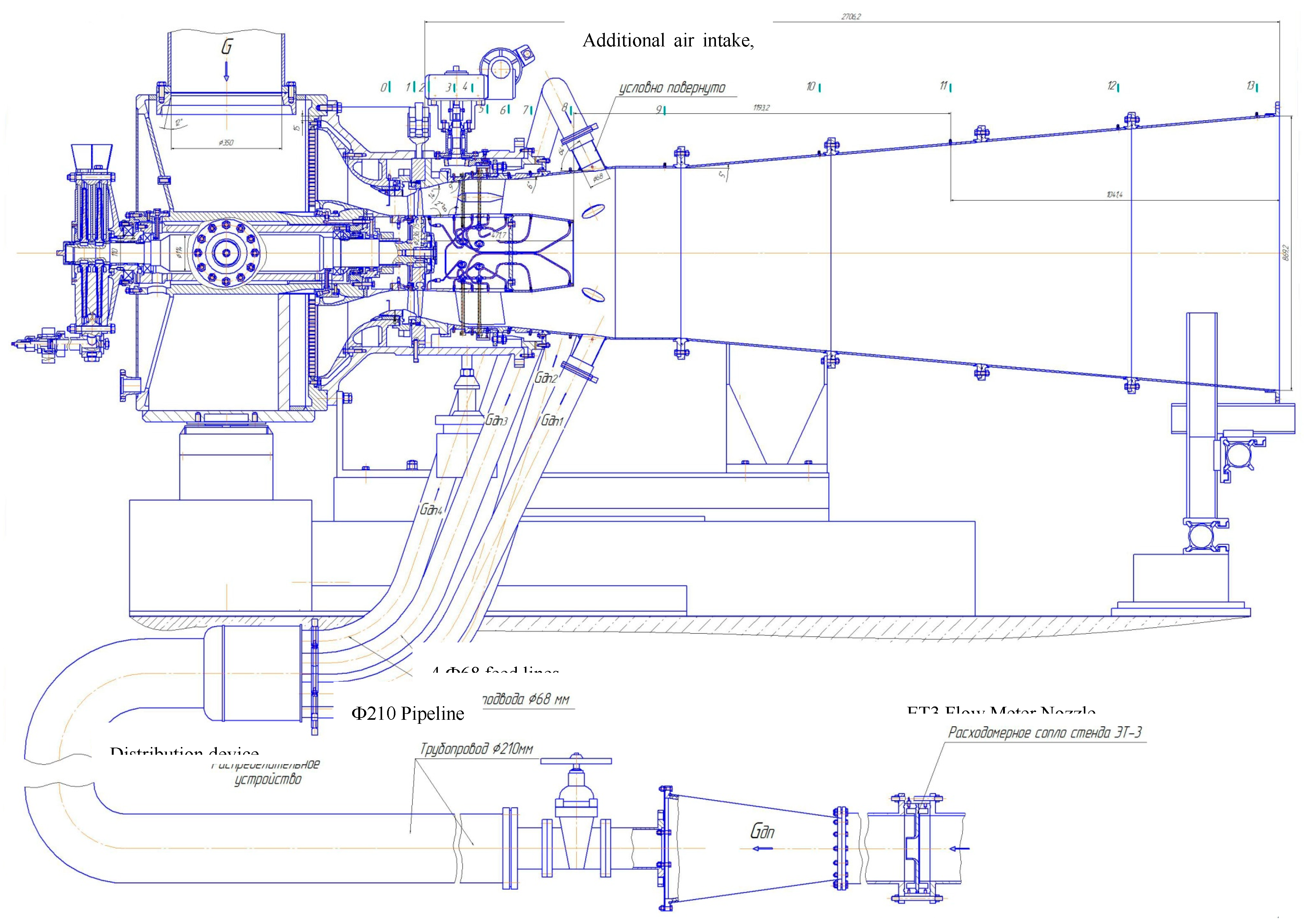
Figure 2.2.
Inputs for additional air intake into the diffuser.
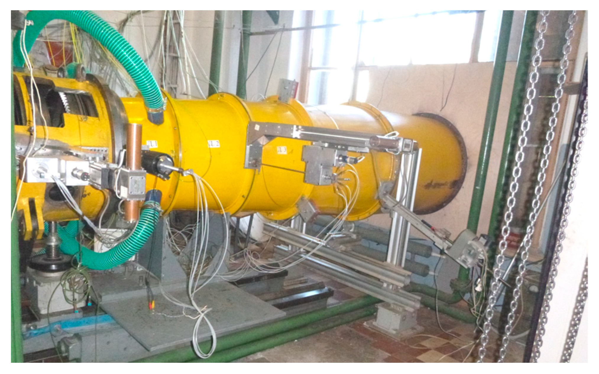
Figure 2.3.
Supplying additional air to the distribution device of the ET4 test bench.
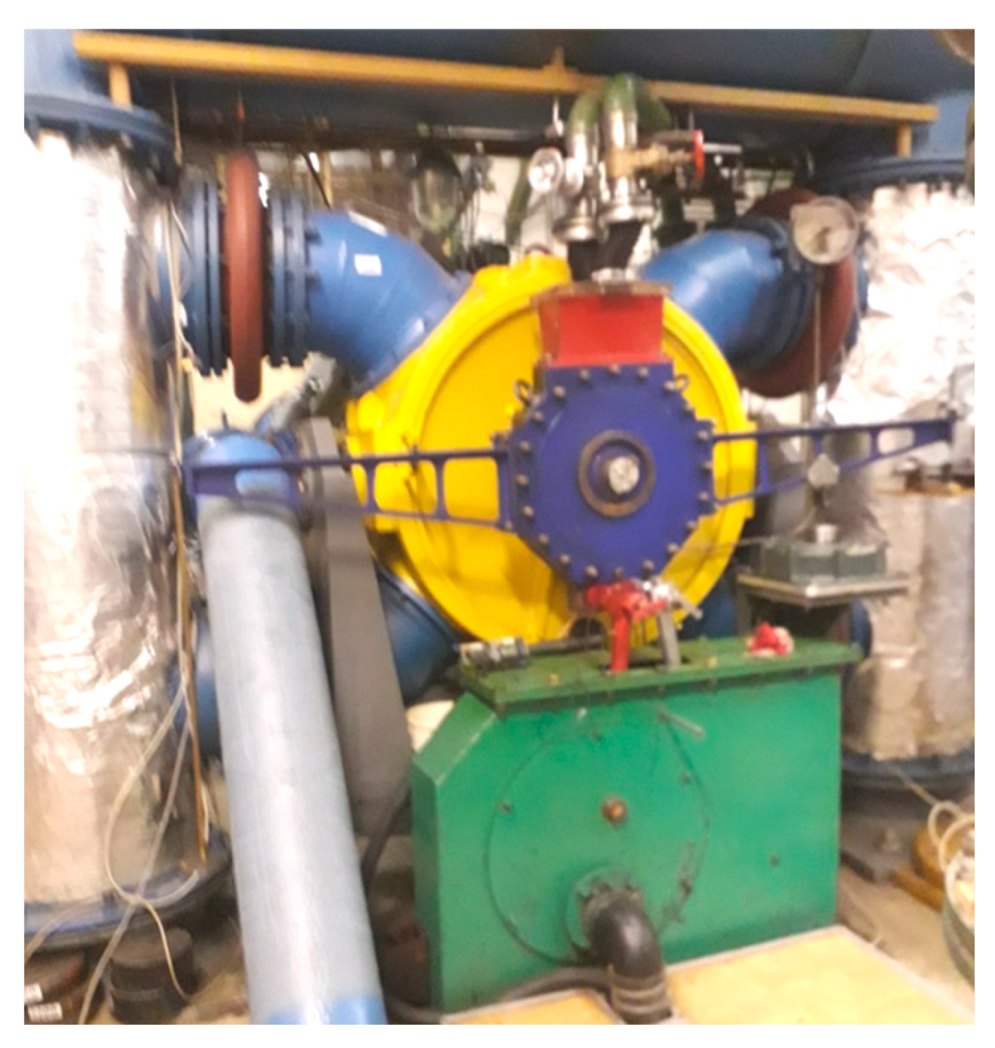
Figure 2.4.
Receiver with air filter of ET3 stand and outlet pipeline of additional blown air.
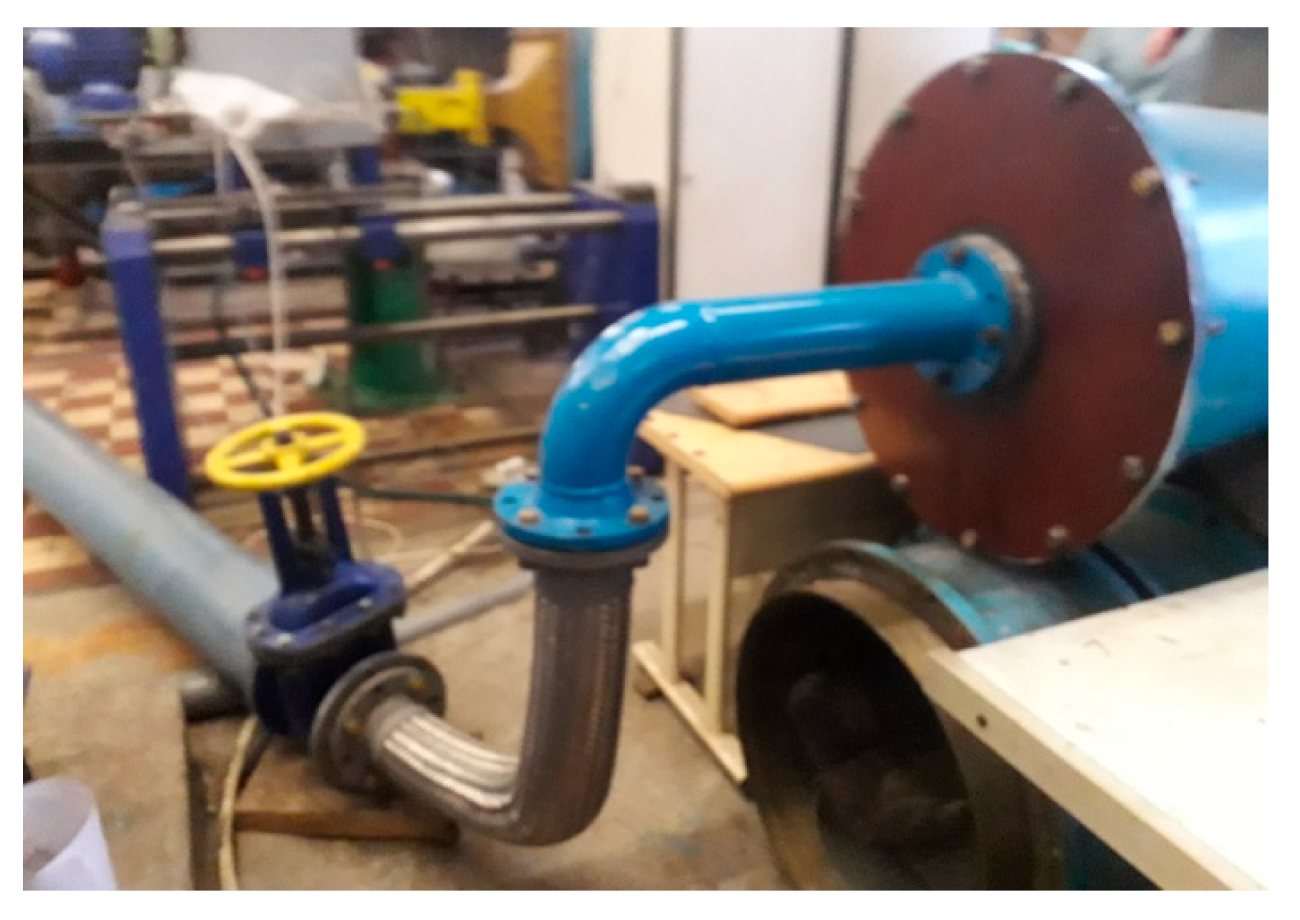

Table 2.1.
Similarity criteria.
| Value | Designation | Dimension | Object | |
| Actual GTU | Model 1:4,566 | |||
| Working fluid | - | - | Combustion products | Air |
| Gas constant | R | Joule/kg. К | 291,17 | 287,1 |
| Isentropic exponent | k | - | 1,3210 | 1,40 |
| Angular velocity | n | rpm | 5441 | 15000 |
| Mach number in section 2-2 | M2 | - | 0,4342 | 0,4112 |
| Mass flow rate | G | kg/sec | 180,8 | 13,5 |
| Reynolds number | Re2 | - | 5,07⋅106 | 1,4⋅106 |
| Characteristic number | u/C0 | - | 0,689 | 0,609 |
| Flow coefficient | cz/u | - | 0,5632 | 0,5631 |
The difference in the Reynolds number that we observe between the actual GTU (5,4.106) and the model ET4 (1,4.106) should not alarm us since for such Mach numbers that are observed in both flows (M2~0,4 Mach) and for these values of the Reynolds numbers we are in the area of auto/selfmodelling of the flow where such differences, do not actually affect the similarity criteria[7] (pp37,38).
2.2. Measurement Diagram
The measurement scheme of the test bench ET4 with the ‘S-D’ model is shown in Figure 2.5 and 2.6. It covers all measurements necessary to determine the integral characteristics of the ‘S-D’ system and to study the 3D flow in its flow path. For this purpose, 11 cross-sections in the diffuser were selected – from cross-section 2-2 at the diffuser inlet to cross-section 13-13 at the outlet. All cross-sections can be divided into two parts: cross-sections with flow traversing, including wall pressure measurements, and cross-sections with circumferential wall pressure distribution measurements using pressure taps.
Wall pressures were measured in all fourteen cross-sections (including cross-sections 0-0 and 1-1). Flow traversing was performed in sections 2-2 behind the rotor blades, 7-7 behind the power struts, 8-8 behind the sleeve diffuser, 11-11 in the middle of the conical section of the diffuser, and 13-13 at the diffuser outlet (Figure 2.5). For this purpose, six coordinate devices with 3D probes were installed in these sections. Traversal of the control sections was typically performed at 11 to 15 points along the radius and from 6 (sections 2-2) to 9 points (sections 7-7 and 13-13) along the angular step.
A preliminary analysis of the flow structure using a numerical experiment revealed a significant potential influence of the power struts on the flow state in section 2-2. Therefore, traversing the inlet cross-section 2-2 and flow traversing in all other control cross-sections (7-7, 8-8, 11-11, 13-13) were performed separately, i.e., sequentially.
Figure 2.5.
Measurement diagram of the ET-4-XX test bench with the high power stationary GTU ‘S-D’ system model and additional air supply to the conical diffuser.
Figure 2.5.
Measurement diagram of the ET-4-XX test bench with the high power stationary GTU ‘S-D’ system model and additional air supply to the conical diffuser.
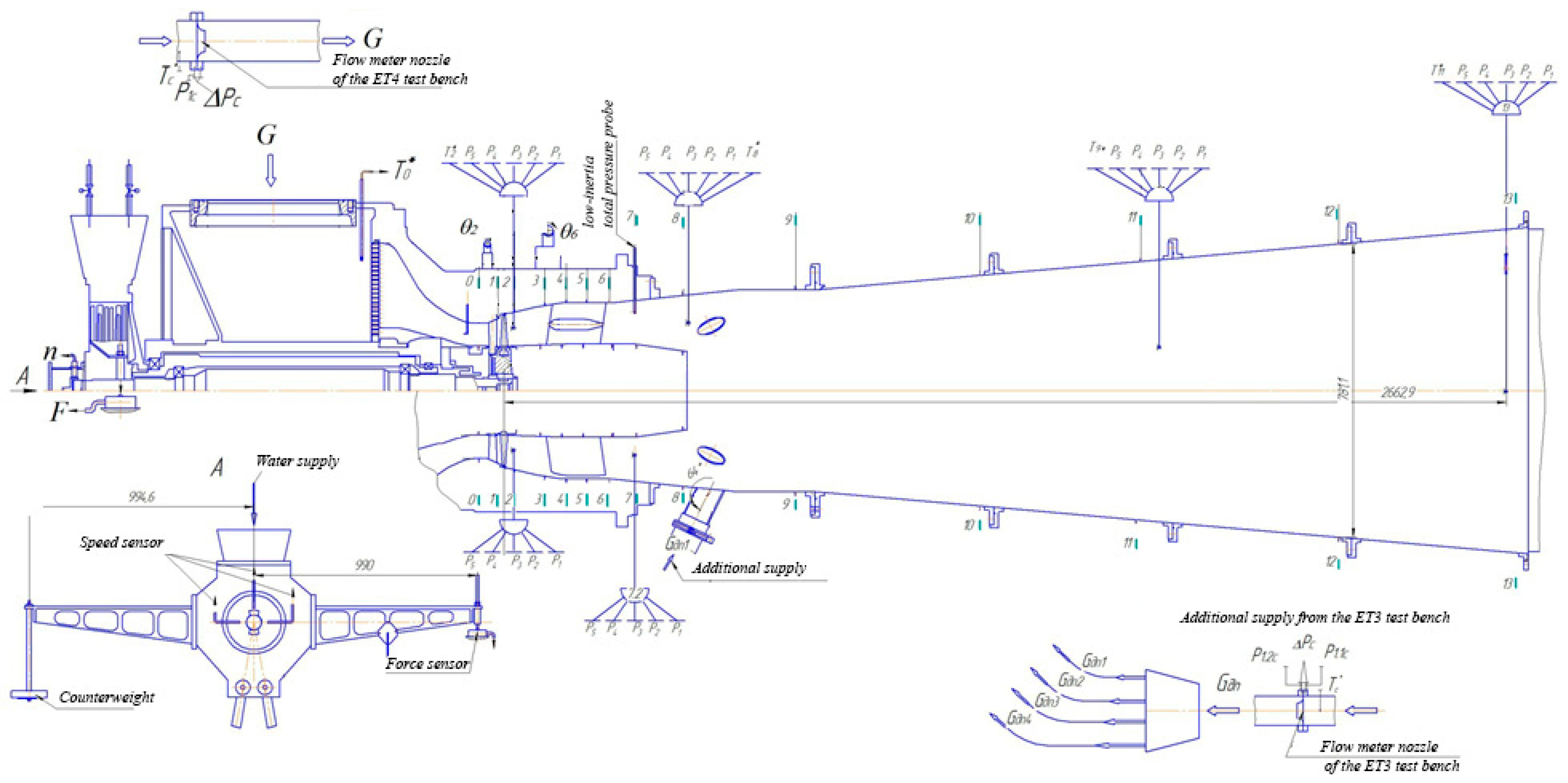
Figure 2.6.
Measuring sections of the ET-4-XX test bench with additional air supply to the conical diffuser.
Figure 2.6.
Measuring sections of the ET-4-XX test bench with additional air supply to the conical diffuser.
2.3. Methodology for Processing Experimental Data
The method of processing experimental data includes calculations as an integral aerodynamic characteristic of the ‘S – D’ system (η+dif, η*+dif), as its components (η, η*), where for example the sign “η+diff” corresponds to the parameter of the efficiency of the system calculated “with” the presence of the diffuser at the exit of the diffuser. And the “η*+diff” corresponds to the efficiency of the “S-D” system calculated at the exit of the diffuser according to the total/braking parameters of the working medium.
Efficiency of the system ‘S-D’ η+ dif и η*+ dif:
where ω - the impeller angular frequency, rad/s;
М – torque developed by the impeller with force F on the hydraulic brake lever (Figure 2.5 and 2.6), N·m;
G – mass flow measured by the flow meter nozzle of the ET4 test bench kg/s;
H0+dif - isentropic enthalpy drop from the total parameters in the inlet of ‘S-D’ system to the pressure in the flow behind diffuser, in section 13-13 (see Figure 2.5 and 2.6), J/kg;
H*0+dif - isentropic enthalpy drop from the total parameters p*0, T*0 in inlet of the ‘S-D’ system to the total parameters behind diffuser, in section 13-13 (see Figure 2.5 and 2.6), J/kg.
Efficiency of the step η, и η*:
where H0 - isentropic enthalpy drop from the total parameters in the inlet of ‘S-D’ system to the pressure in the flow behind step, in section 2-2 (see Figure 2.5 and 2.6), J/kg;
H*0 - isentropic enthalpy drop from the total parameters in the inlet of ‘S-D’ system to the pressure in the flow behind step, in section 2-2 (see Figure 2.5 and 2.6), J/kg.
The pressure recovery coefficient in the diffuser of the ‘S - D’ system is determined by the formula:
where p2 and p13 are the average pressures in control measurement sections 2-2 and 13-13 respectively (see Figure 2.5 and 2.6); and is the dynamic pressure in section 2-2 at the diffuser inlet.
The efficiency of the diffuser, equal to the effective pressure recovery coefficient of the diffuser Cpeff, is determined by the formula:
where - ideal recovery coefficient, determined by the ratio of the inlet (F2) and outlet (F13) cross-sections of the diffuser.
p13 – average pressure at the outlet of the diffuser in section 13-13 (Figure 2.5 and 2.6), Pa;
ρ2, с2 – average density and flow velocity in section 2-2 behind stage (Figure 2.5 and 2.6) kg/m3 and m/s;
p*0 - average total pressure in the flow before the ‘S-D’ system (Figure 2.5 and 2.6), Pa.
2.4. Measuring Instruments and Equipment
The ET4 test bench is equipped with an automated information and measurement system that provides experiment control and data recording [8].
The flow nozzle is located in the supply pipeline upstream of the turbine. Flow measurement is a standard operation, regulated by relevant regulatory documents. The flow nozzle installed on the rig, the temperature and pressure sensors located on it, and the nozzle’s positioning in the pipeline comply with these regulations.
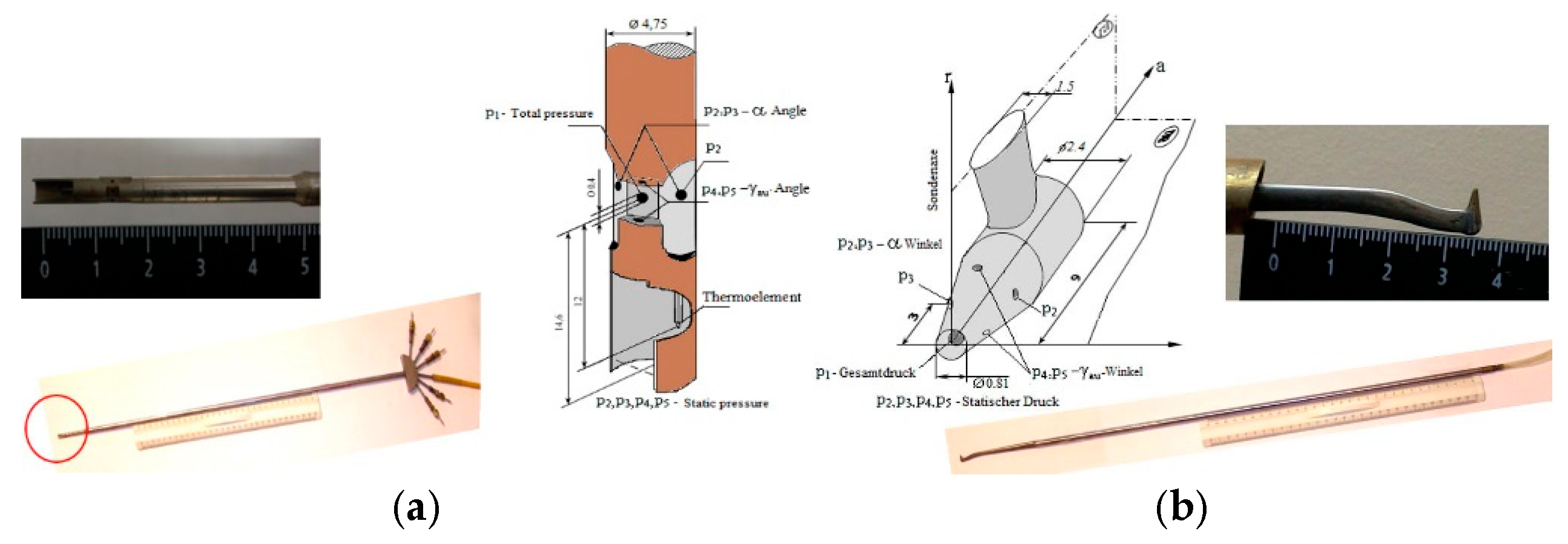
Five-channel pneumometric vector probes (Figure 2.7) are used to traverse the three-dimensional flow in control sections. Measurements are conducted in a semi-oriented mode.
Figure 2.7.
Five-channel Probes: a) - cylindrical United Sensor probe; b) – conical probe.
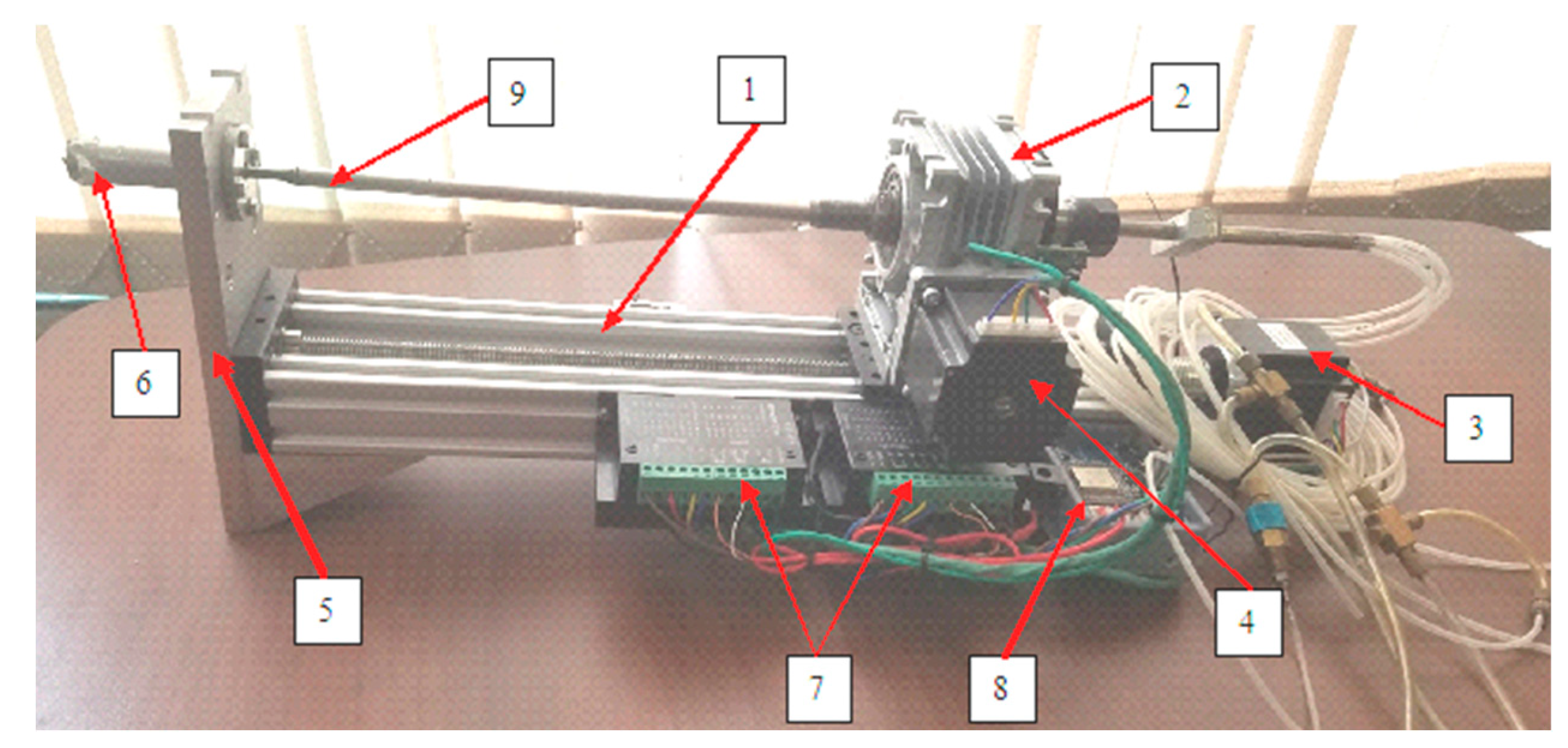
The coordinate devices (Figure 2.8) in which the probes are mounted allow for remote control of the radial and angular position of nozzles. The coordinate device provides a linear displacement accuracy of ±0.01 mm in absolute value and an angular displacement accuracy of ±0.01%.
Figure 2.8.
Coordinate system for orientation of 3D pneumatic probes: 1 - coordinate system guide; 2 - RV-030 gearbox; 3 - stepper motor for linear movements; 4 - stepper motor for angular movements; 5 - bracket; 6 - sealing sleeve; 7 - stepper motor drivers; 8 - controller; 9 - 3D probe.
Figure 2.8.
Coordinate system for orientation of 3D pneumatic probes: 1 - coordinate system guide; 2 - RV-030 gearbox; 3 - stepper motor for linear movements; 4 - stepper motor for angular movements; 5 - bracket; 6 - sealing sleeve; 7 - stepper motor drivers; 8 - controller; 9 - 3D probe.
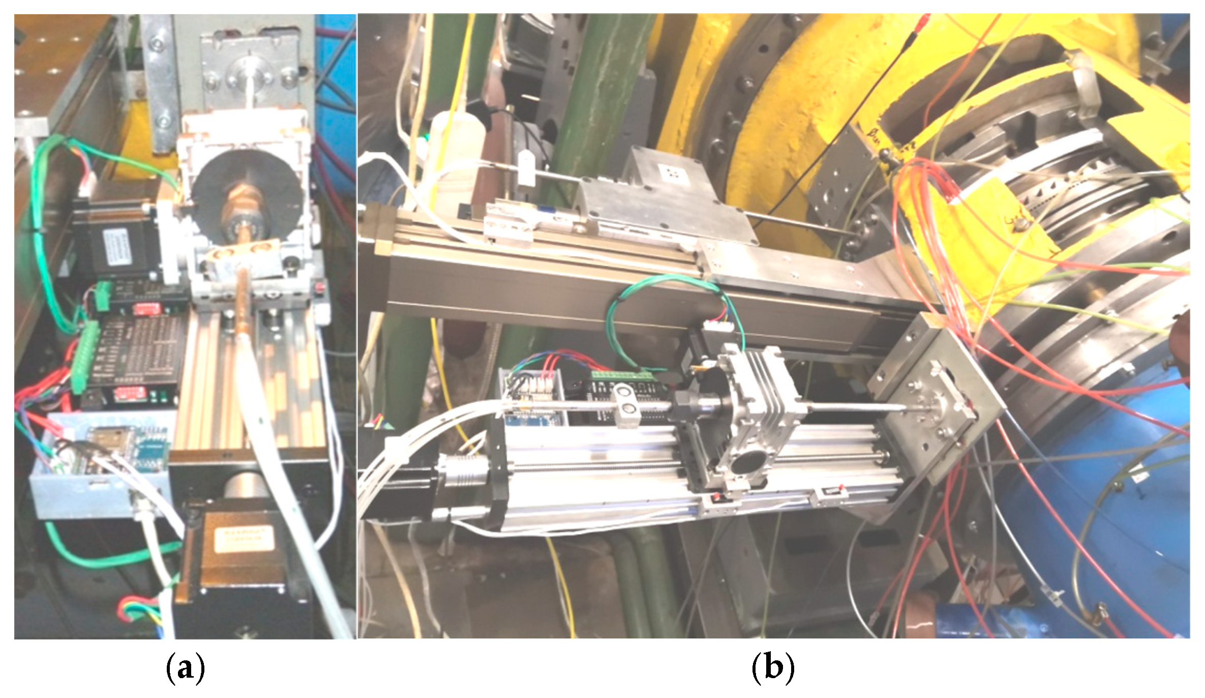
According the measurement scheme (Figure 2.5 and 2.6), the coordinate devices with probes are placed in sections 2-2, 7-7, 8-8, 11-11 and 13-13 (see photo in Figure 2.9).
Figure 2.9.
Coordinate devices with probes on the ET4 test bench: a) – section 2-2; b) – sections 6-6 and 7-7.
Figure 2.9.
Coordinate devices with probes on the ET4 test bench: a) – section 2-2; b) – sections 6-6 and 7-7.
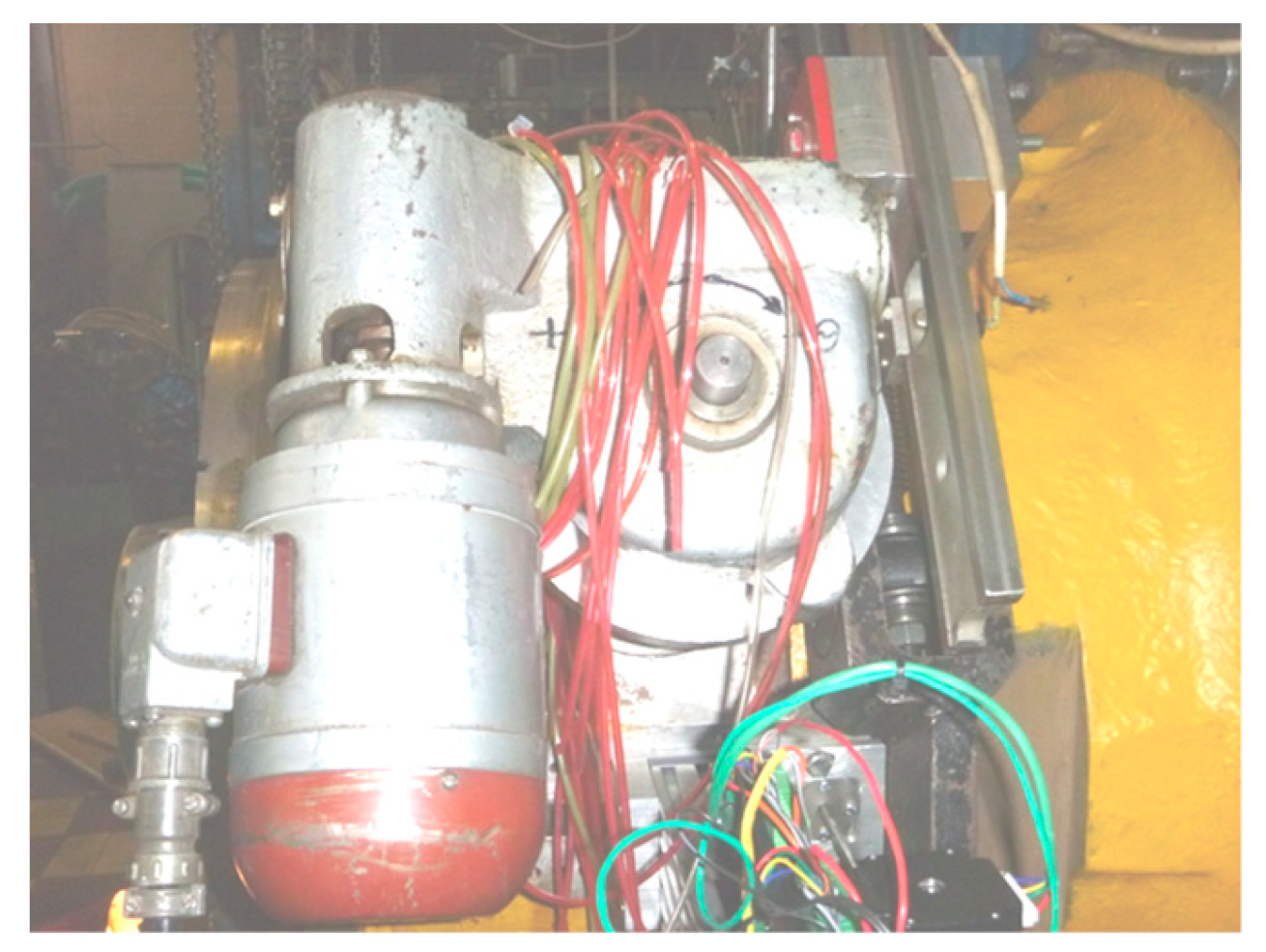
The θ2 and θ7 coordinates in the ET4 test bench’s polar coordinate system were achieved by rotating the guide vane by an angle of θ2i and the sleeve diffuser with power struts by an angle of θ7i, which were registered using video cameras. Special mechanisms with electric drives were used to rotate these components (Figure 2.10 and 2.11).
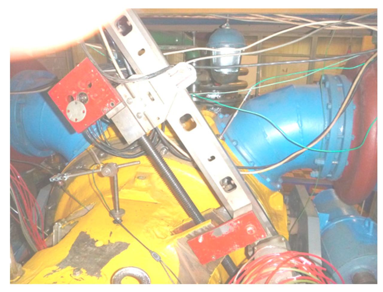
Figure 2.10.
Figure 2.11.
Drive mechanisms for setting coordinates θ2 and θ7.
The 901x series pneumatic intelligent pressure scanners [9] are used to convert pressures measured during an experiment into digital code and support data transmission via a local area network interface using the TCP/IP protocol.
2.5. Calculation Model
The aerodynamics of the ‘S-D’ system were modelled based on the similarity criteria between the actual and model flow in full range of the load modes.
The research was conducted using numerical modelling of actual and model flows. The modelling area also included the outlet diffuser. The calculations were preliminary in nature and were performed without taking into account the cooling of the turbine blade assembly. The objective of the numerical modelling was to obtain the closest possible match between the structure of the model flow and the actual flow in the impeller of the last stage of the turbine and in the outlet diffuser. In this regard, the modelling was carried out in several stages. First, the actual flow in the entire turbine together with the outlet diffuser was modelled (Figure 2.12). Using this model, the parameters before the third stage were obtained. Then, the actual flow in the ‘3-4 stage - outlet diffuser’ compartment was modelled in more detail (Figure 2.13).
Figure 2.12.
Numerical model of natural flow in the turbine-diffuser system.
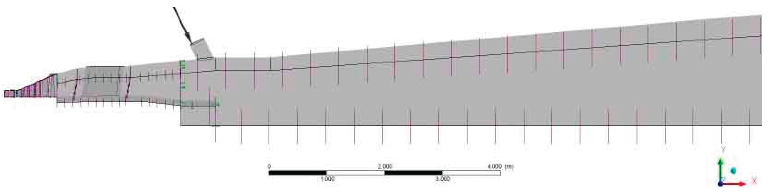
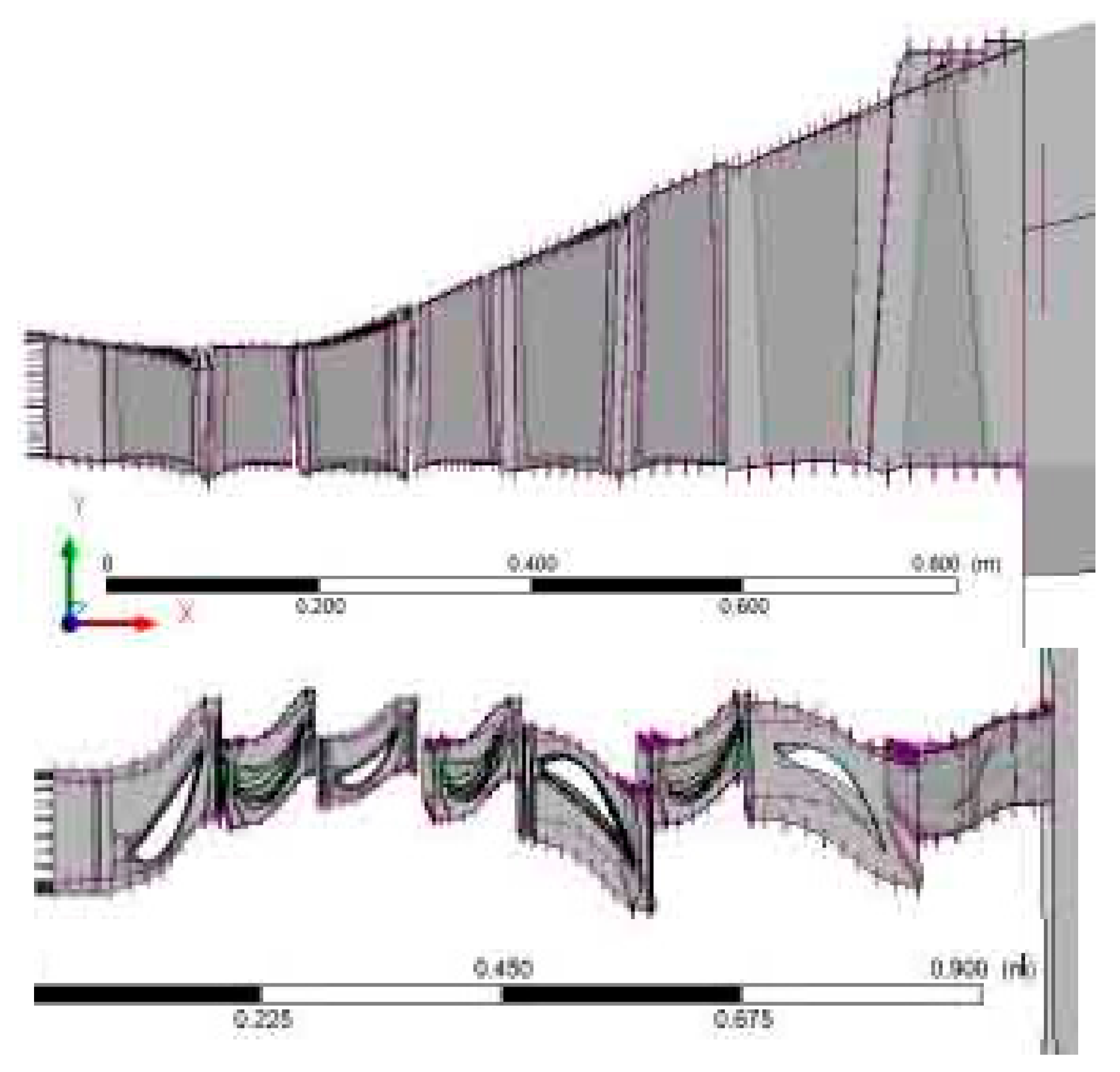
Figure 2.13.
Numerical models of flow in the ‘3-4 turbine stages – diffuser’ system: a) – actual; b) – model.
Figure 2.13.
Numerical models of flow in the ‘3-4 turbine stages – diffuser’ system: a) – actual; b) – model.
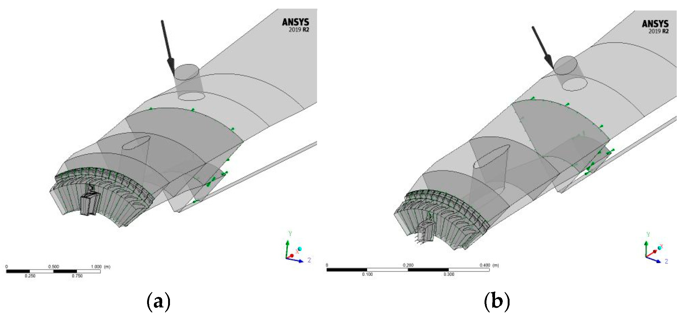
As a result, of preliminary numerical modelling, the main parameters of the model experiment for simulating the specified modes on the Last Stage-Diffuser (‘S-D’) model were determined: air flow rate G, rotor speed n, and flow exit angles from the stage α2m at the middle of the diameter d2m. The values of these parameters, as well as the similarity criteria for the actual and model flow at the nominal load mode and for the specified modes of 10% and 0% of the nominal load presented in Table 2.2.
Table 2.
2. Mode parameters and similarity criteria.
| Percentage of load from rated power | |||||||
| Mode parameter | 100% | 10% | 0% | ||||
|
Actual GTU |
Model (ET4) |
Actual GTU |
Model (ET4) |
Actual GTU |
Model (ET4) | ||
| Combustion gases | Air | Combustion gases | Air | Combustion gases | Air | ||
| Working medium gas constant [Joules/kg К] | R | 291,17 | 287,1 | 291,17 | 287,1 | 291,17 | 287,1 |
| Isentropic index | k | 1,321 | 1,4 | 1,321 | 1,4 | 1,321 | 1,4 |
| Flow rate [kg/sec] | G | 168,38 | 11,695 | 85,4 | 4,4 | 75,73 | 3,8 |
| Rotor speed [rpm] | n | 5441 | 11050 | 5441 | 11050 | 5441 | 11050 |
| Exit angle from the impeller on the middle diameter [deg] | α2m | 92,93 | 92,40 | 31,40 | 33,79 | 27,97 | 28,77 |
| Similarity criteria | |||||||
| Mach number | M | 0,430 | 0,344 | 0,457 | 0,340 | 0,471 | 0,340 |
| Characteristic number | u/C0 | 0,653 | 0,578 | 1,592 | 1,365 | 1,880 | 1,631 |
| Thermodynamic reactivity index | ρт | 0,426 | 0,287 | -0,057 | -0,023 | -0,197 | -0,170 |
| Kinematic reactivity index | ρк | 0,311 | 0,214 | 0,018 | 0,038 | -0,014 | -0,004 |
| Circulation coefficient | 1,070 | 1,238 | 0,038 | 0,097 | -0,054 | -0,023 | |
| Flow coefficient | 0,586 | 0,614 | 0,276 | 0,293 | 0,259 | 0,273 | |
| Reynolds number | Re·10-6 | 2,58 | 1,05 | 3,07 | 0,82 | 3,17 | 0,87 |
| Strouhal’s number | Sh | 0,258 | 0,241 | 0,253 | 0,260 | 0,246 | 0,243 |
| Froude number | Fr | 0,178 | 0,204 | 0,185 | 0,175 | 0,196 | 0,200 |
2.6. Mesh Model of the S-D Model System. Numerical Simulation
The geometry of the model flow section of the ‘S-D’ system is shown earlier in Figure 2.12. In order to preserve the angular dimensions of the calculation area along the entire length of the outlet tract, a deviation from the actual geometry was made, which consisted in replacing four additional air supply pipes in the conical diffuser with five pipes equivalent in total passage area. The axial position of the pipe was modeled exactly in accordance with the geometry of the prototype and the modeling scale of 1:4.566.
The calculated area of the model system “S – D” consists of 5 domains. The domain of the 4th stage guide apparatus (GV) includes 10 interblade channels, and the domain of the 4th stage impeller (RB) includes 15 interblade channels. The ring diffuser domain covers the inter-blade space of the ring diffuser with an angular extent of 360°/5=72°. The conical diffuser domain is a segment of the conical part of the diffuser with an angular extent of 72° with an additional air supply pipe. A numerical model of the ‘S-D’ system is shown in Figure 2.14.
Figure 2.14.
Numerical model of the ‘S – D’ system.
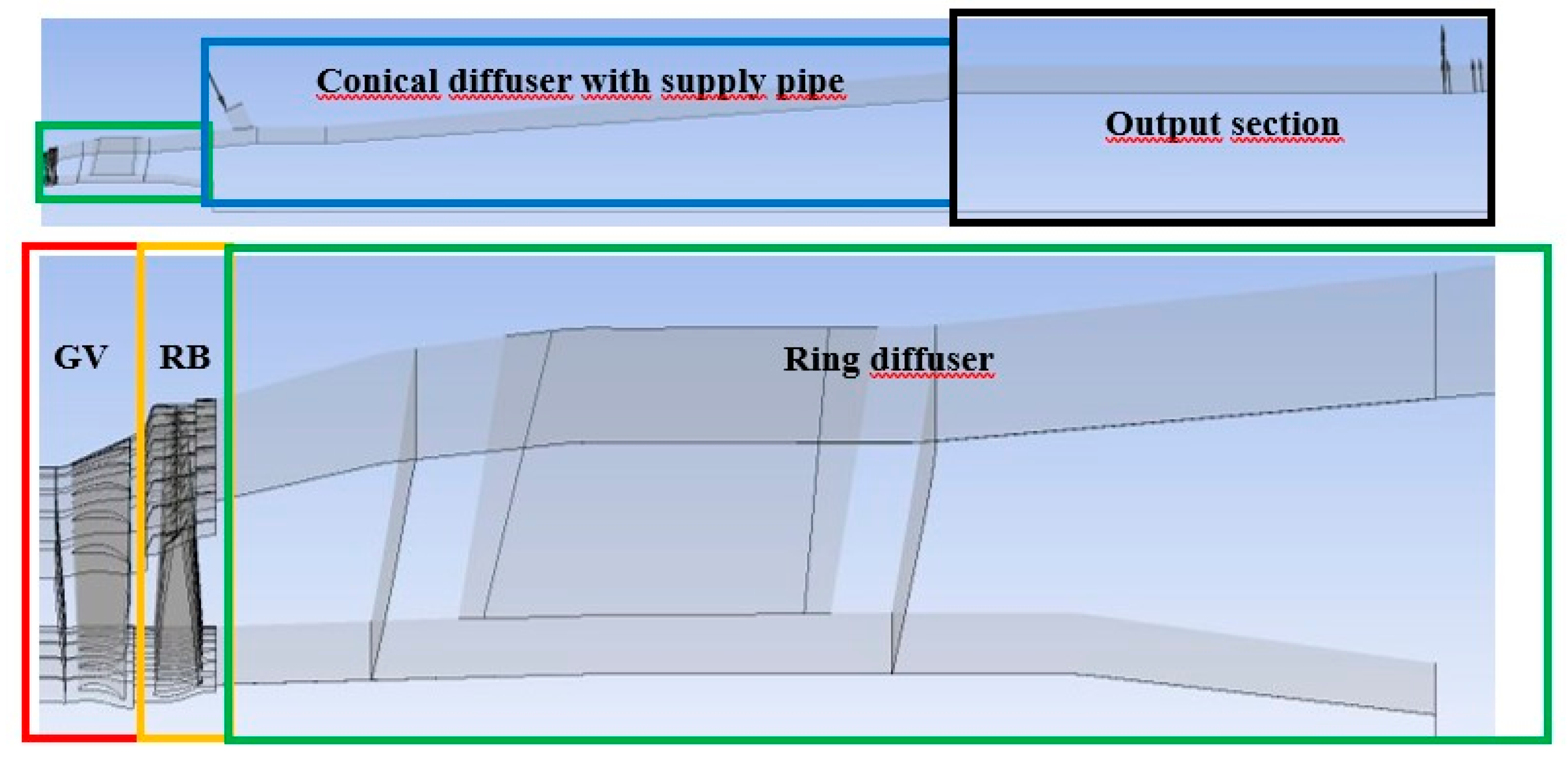
The calculation grids on the surfaces of the fourth stage sleeve and blades are shown in Figure 2.15, and on the surfaces of the annular and conical diffusers – in Figure 2.16 and 2.17.
Hexahedral meshes were used in all areas of the computational model, except for the peripheral area of the working blade.
Figure 2.15.
Mesh on the surface of the sleeve and blades of the fourth stage.
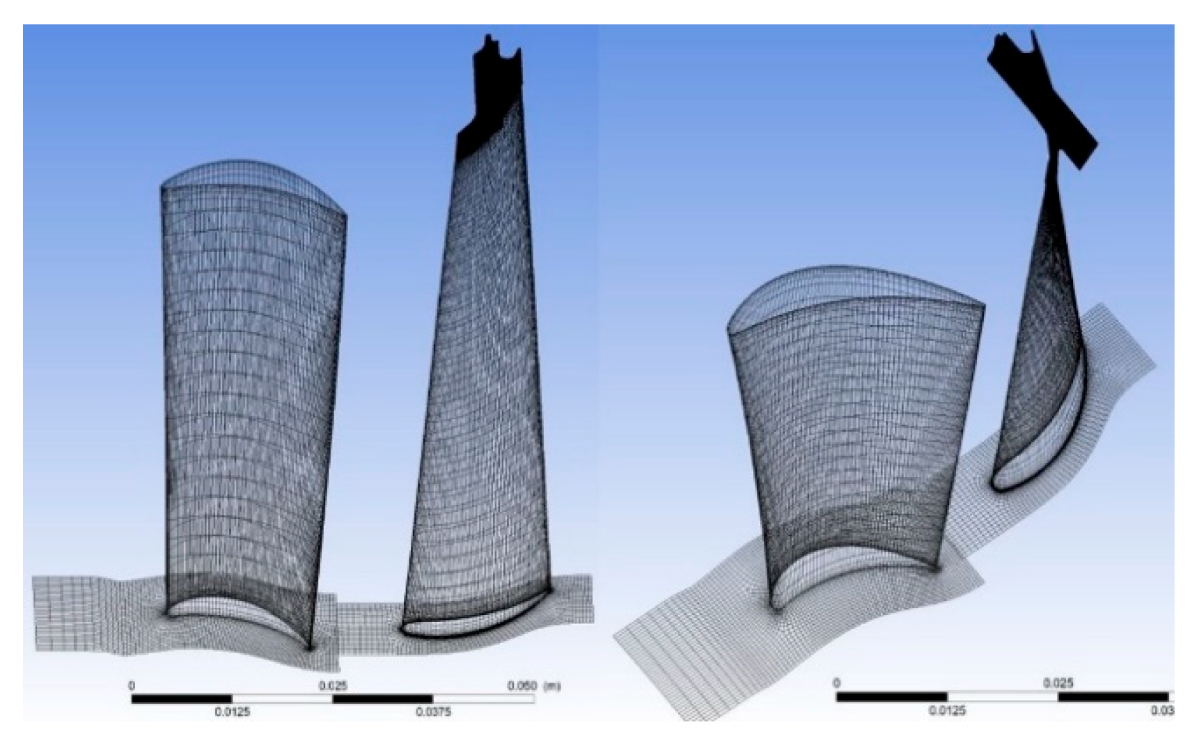
Figure 2.16.
Mesh on the surfaces of the power stand and ring diffuser.
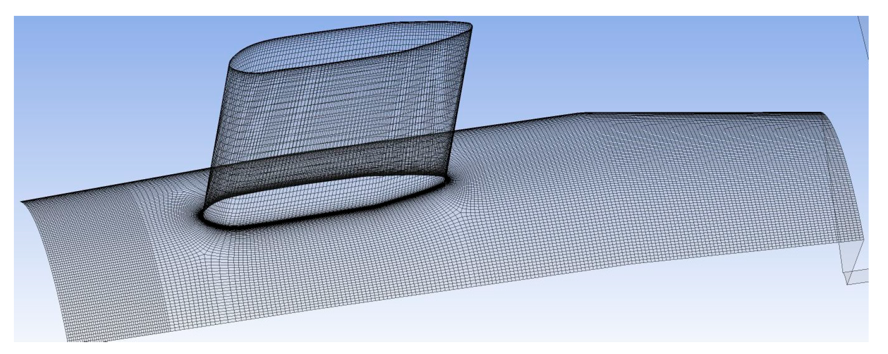
Figure 2.17.
Mesh on the surfaces of the peripheral contour of a conical diffuser with additional air supply.
Figure 2.17.
Mesh on the surfaces of the peripheral contour of a conical diffuser with additional air supply.
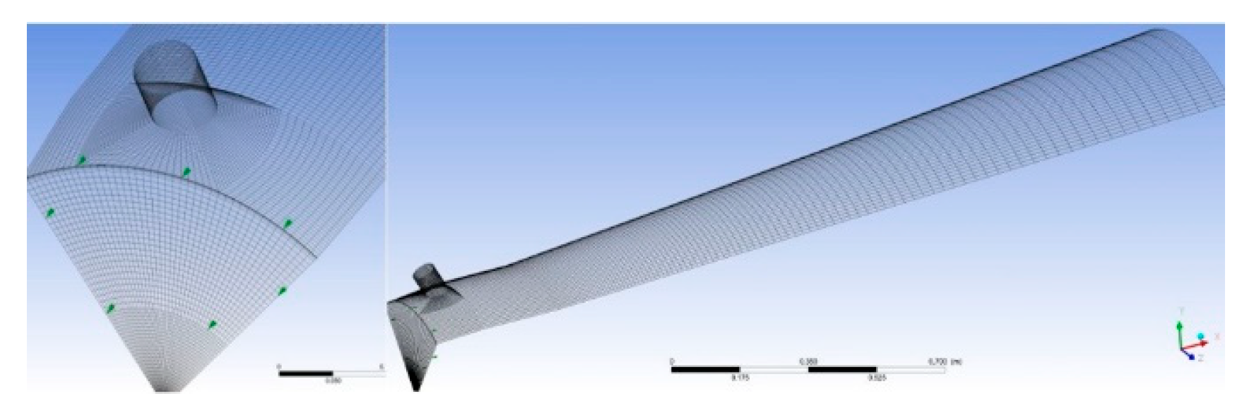
The parameters of the mesh models are presented in Table 2.3. The total size of the computational mesh, including the outlet cylinder mesh, was 17.8 million nodes and 33.2 million elements.
Table 2.3.
Grid model parameters.
| Domain | Mesh type | Number of nodes | Number of Elements |
| GV | Hexahedra | 2312390 | 2181400 |
| RB | Hexahedra, Tetrahedra | 13939440 | 29526540 |
| Ring diffuser | Hexahedra | 922908 | 887158 |
| Conical diffuser | Hexahedra | 397598 | 375474 |
2.7. Numerical Model of Flow in the System ‘S – D’
When calculating the model flow in the ‘S-D’, the boundary conditions at the inlet of the 4th stage (p*0 and T*0) were taken from a model experiment in which the load mode was determined by the given value of the flow outlet angle at the middle diameter behind the impeller. The inlet to the additional air supply pipe the flow rate through a single pipe Gadd.air/5 and total temperature T*add.air were set.
To simulate the flow in the ‘S-D’ system under partial load conditions, the DES method was chosen, which partially resolves the vortex structure of the flow. A second-order upwind scheme was used to discretize convective flows, and time operators were discretized with a second-order approximation. The time step was 4.5·10-6 s, which corresponded to the rotor displacement by one interblade channel in 20-time steps. At each time step, 10 iterations were performed. In the calculation models of the ‘S-D’ system, a model of an average steady turbulent flow of compressible gas was adopted. The flow is described by Reynolds-averaged Navier-Stokes (RANS) equations and energy equations. To describe turbulence, the Boussinesq hypothesis was adopted, and turbulent viscosity is described by the SST turbulence model of Menter.
In the GV channels and in the diffuser, the flow is considered in a stationary coordinate system, and in the RB channels, in a rotating coordinate system. The calculations were performed using the ANSYS CFX [10] software package. Spatial and temporal discretization is performed with second-order accuracy.
The numerical model of flow in the full-scale system “S – D” differs from the model only in the properties of the working fluid [11] (pp96-408). The molar mass of combustion products is assumed to be 28.4 kg/kmol. The heat capacity is specified as an interpolation dependence on temperature based on the set of points in table form. Dynamic viscosity and thermal conductivity are determined using the Sutherland formula. Gas viscosity:
where T0=273,15 oK, μ0=1,715.10-5 Pa.s, C=110,6oK.
Thermal conductivity of gas:
where T0=273,15 oK, λ0=0,02414 W/(m.oK), C=194,4oK.
Numerical simulations of the actual flow were performed for three gas turbine load conditions: nominal (100%), 10% of nominal load, and gas turbine idle (0%). The basic parameters (flow rate, total inlet temperature, and inlet pressure) were provided by the Customer. The initial data for the investigated modes are presented in Table 2.4.
Table 2.4.
Initial parameters of the calculated modes/operating regimes.
| Parameters | Operating mode | |||
|
№1 100% |
№2 10% |
№3 0% |
||
| GTU Power [NТ] | kW | 141306 | 37993 | 29435 |
| Rotor speed [n] | rpm | 5441 | 5441 | 5441 |
| Mass flow rate [G] | kg/sec | 150,6 | 75,88 | 66,88 |
| Brake pressure at the turbine inlet [P*in] | bar | 14,95 | 6,66 | 5,79 |
| Brake temperature at the turbine inlet [Т*in] | oК | 1589 | 1210 | 1157 |
| Pressure at the diffuser outlet [Pout] | Pa | 91129 | 91129 | 91129 |
The flow rate and braking temperature were specified as input boundary conditions. The average cross-sectional pressure was specified at the outlet. The shaft rotational speed remained constant at n = 5441 rpm for all calculations. Adhesion and adiabatic conditions were specified for all solid surfaces. For the nominal operating mode, additional calculations were performed taking into account the non-uniform parameter field at the inlet to the 4th stage: a calculation with an inlet velocity and temperature profile, as well as flow simulation in the ‘S–D’system, which includes all four turbine stages and the outlet diffuser.
3. Results
3.1. Integral Characteristics of the Last Stage- Diffuser ‘S–D’ System
In accordance with the measurement diagram shown in Figure 2.5, probes 21 and 22 (section 2-2), positioned diametrically opposite, and probe 8 (section 8-8) are used to traverse the flow in control sections 2-2 and 8-8. Based on the results of averaging the flow parameters in section 2-2 and the boundary conditions P0*, T0* and P13, the integral characteristics of the stage and the ‘S–D’ system were calculated for the specified load conditions.
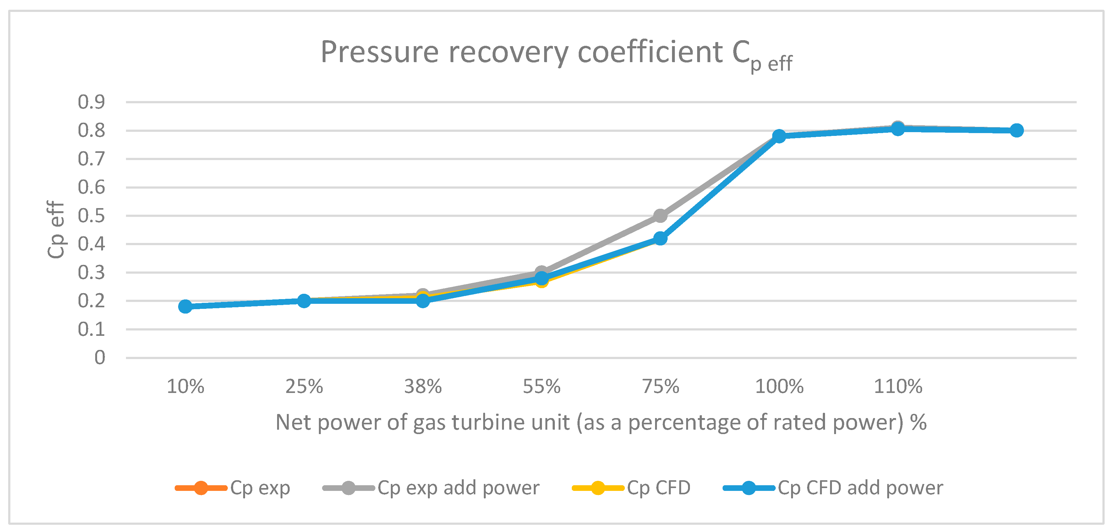
The results obtained are presented in the form of graphs showing the variation in the efficiency of the stage and the ‘S–D’ system, as well as the diffuser pressure recovery coefficient in the load range from 110% to gas turbine idling, are presented in Figures (Figure 3.1 and 3.2) [9].
Figure 3.1.
Changes in the efficiency of the stage and the ‘S–D’ system based on the results of a simulation
experiment and numerical simulation(CFD) across a load range from 110% of rated power to gas turbine idling.
Figure 3.1.
Changes in the efficiency of the stage and the ‘S–D’ system based on the results of a simulation
experiment and numerical simulation(CFD) across a load range from 110% of rated power to gas turbine idling.
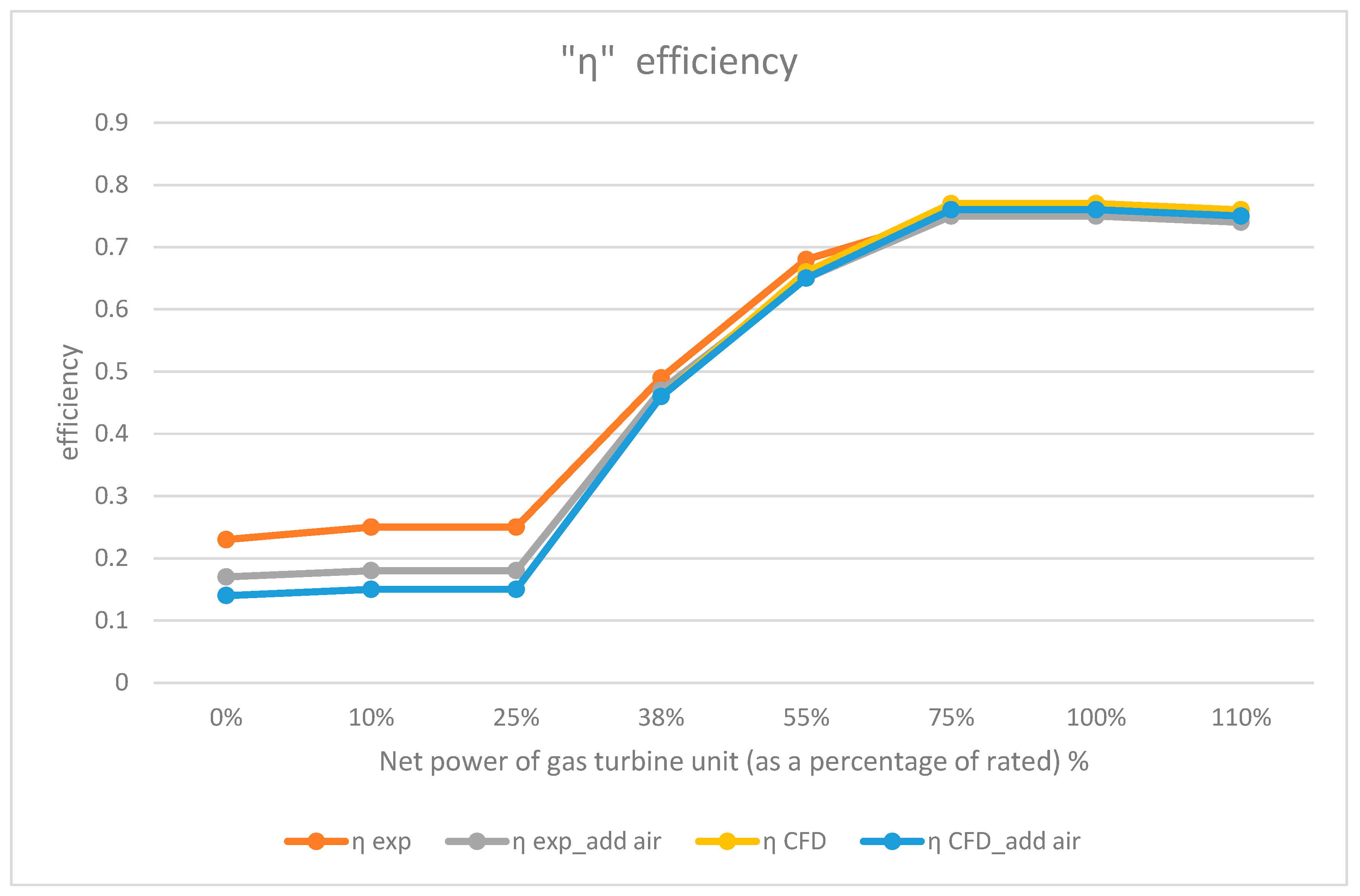
Figure 3.2.
Change in the recovery coefficient Cp eff based on the results of a simulation experiment and CFD
analysis across a load range from 110% of rated power to gas turbine idling.
Figure 3.2.
Change in the recovery coefficient Cp eff based on the results of a simulation experiment and CFD
analysis across a load range from 110% of rated power to gas turbine idling.
The integral characteristics of the stage, diffuser and ‘S–D’ system at rated load (100%) are shown in Table 3.1.
Table 3.1.
Integral characteristics of the last stage- diffuser ‘S–D’ system at nominal conditions.
|
Nr. |
Variable | symbol | Actual GTU | Model ‘S-D’ | |
|
Calculation RANS |
Experiment | ||||
| 1 | Rotation speed [rpm] | n | 5441 | 11050 | |
| 2 | Flow rate of the working fluid at the 4th stage, [kg/s] | G | 194 (195) | 11,7 | 11,67 |
| 3 | Air flow rate through the diffuser, (%) [kg/s] | Gadd. Air | 0 | 0 | 0 |
| 4 | Characteristic number [-] | u/C0 | 0,692 | 0,632 | 0,616 |
| 5 | Flow angle at the mean diameter in section 2-2, [o] | a2c | 94 | 93,0 | 93,8 |
| 6 | Mach number at the mean diameter in section 2-2 [-] | М2 | 0,462 | 0,344 | 0,325 |
| 7 | Power of the 4th stage, [kW] | N4 | 31300 | 485 | 374 |
| 8 | Pressure recovery coefficient in the diffuser, [%] | Cp | 83,9 | 81,4 | 82,3 |
| 9 | Stage efficiency, [%] | η | 77,4 | 75,8 | 75,9 |
| 11 | Efficiency of the ‘S-D’ system, [%] | η +diff | 91,0 | 87,6 | 88,0 |
In section 2-2, located downstream of the impeller at the diffuser inlet, the sweep was carried out using two probes positioned diametrically opposite each other. Section 8 at the outlet of the annular diffuser was swept using a single probe.
Traversing the flow in increments of GV with the power struts in a fixed position showed no stepwise irregularity in the inlet section of the diffuser. At the same time, a difference was recorded in the readings from the probes in section 2-2. In section 8-8, the traversal results could not be processed due to the turbulent nature of the flow. Consequently, it was decided to traverse the control sections only along the pitch of the struts. Figure 3.3–3.5 show the distribution of flow parameters by the channel height in section 2-2 under operating conditions of 10% of the nominal load at Gadd.air=0. Similar measurements were carried out in all control sections for all load modes presented in the graphs of integral characteristics 3.1 - 3.2 at Gadd.air=0 and Gadd.air=11.2%.
Figure 3.3.
Variation of pressure and temperature along the height of the duct in section 2-2. 10% mode, Gadd.air=0.
Figure 3.3.
Variation of pressure and temperature along the height of the duct in section 2-2. 10% mode, Gadd.air=0.
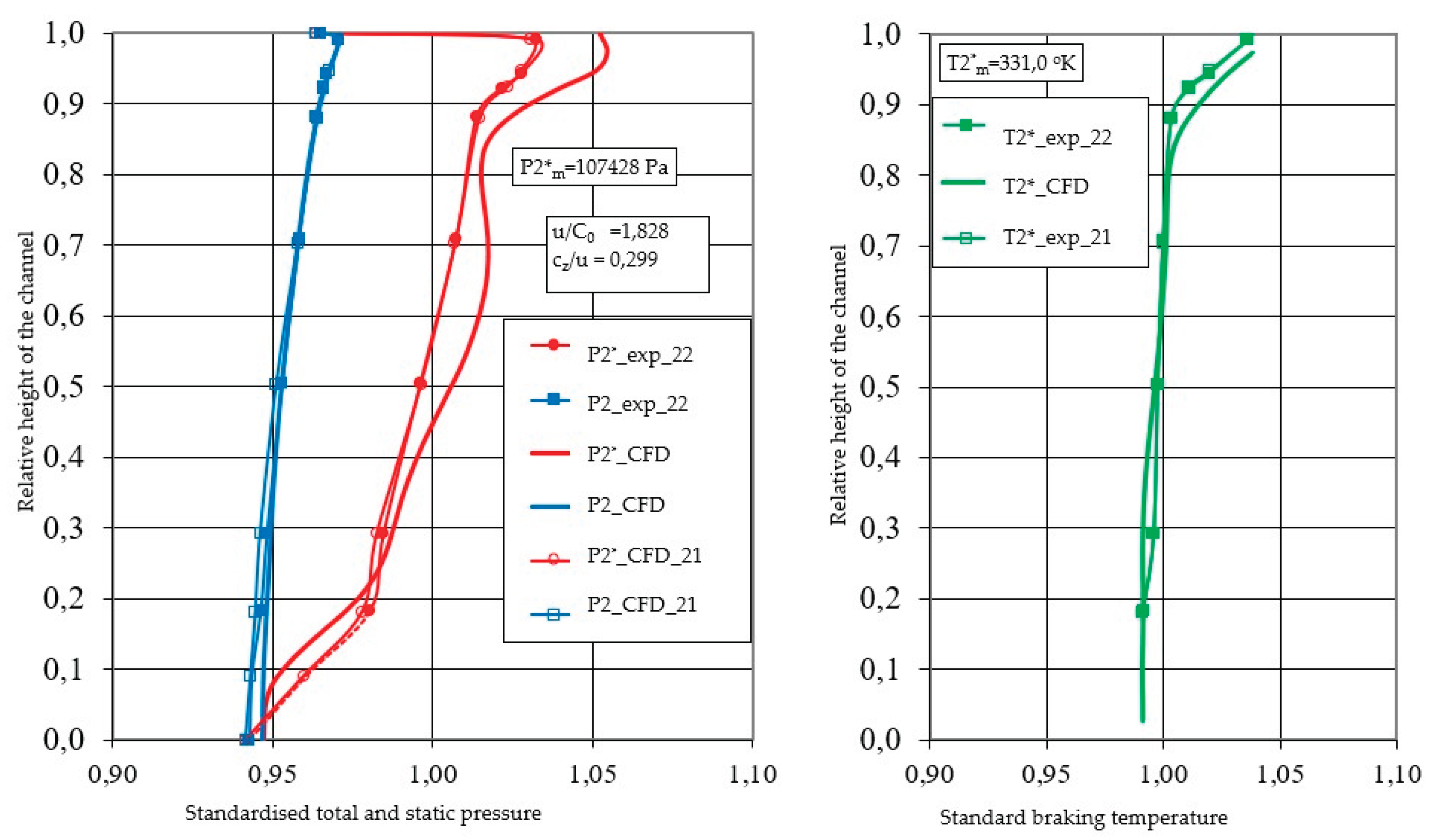
Figure 3.4.
Variation of the components of the Mach number along the height of the channel in section 2-2. 10% mode, Gadd.air=0.
Figure 3.4.
Variation of the components of the Mach number along the height of the channel in section 2-2. 10% mode, Gadd.air=0.
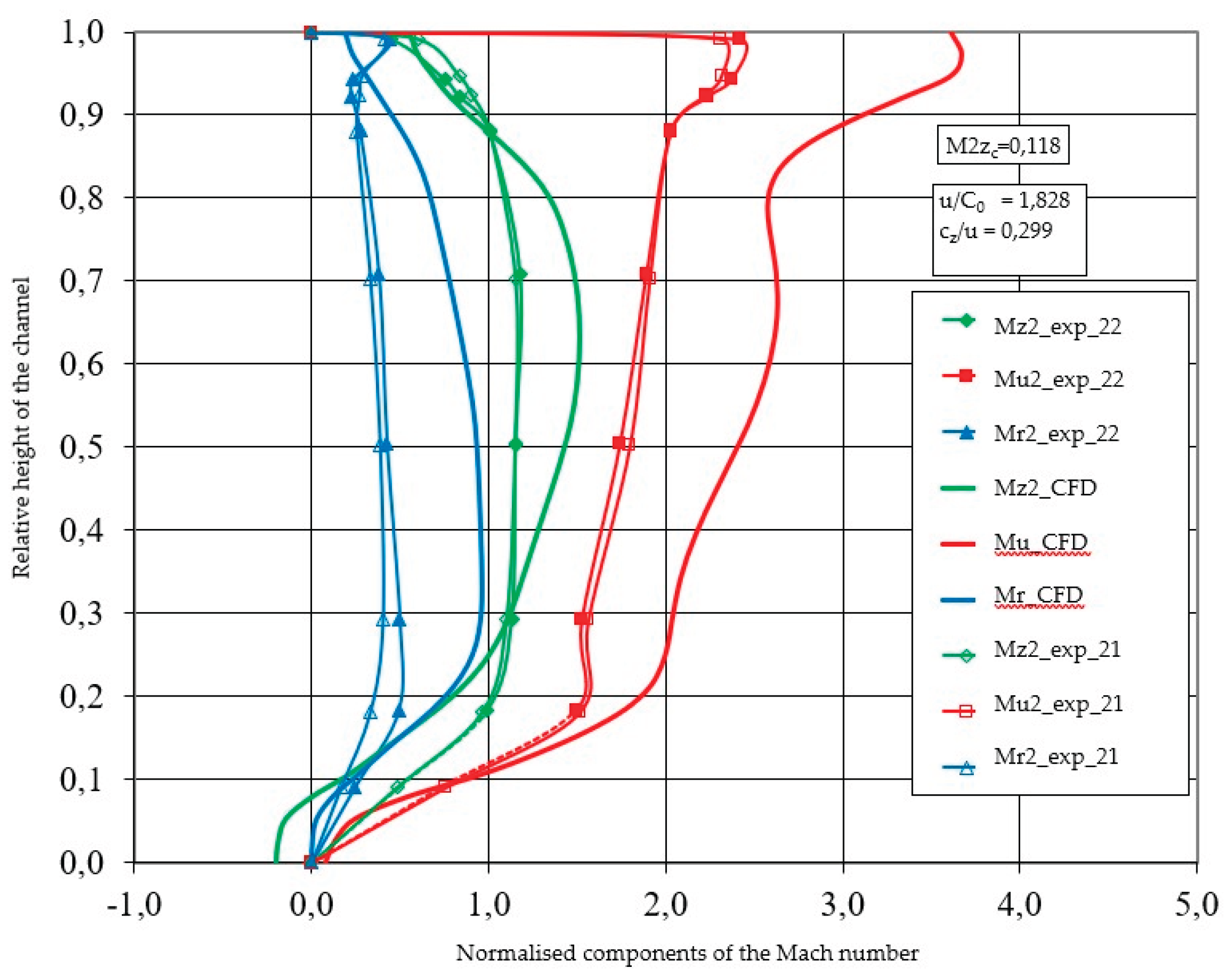
Figure 3.5.
Variation in mean flow angles along the height of the channel in section 2-2. 10% mode, Gadd.air=0.
Figure 3.5.
Variation in mean flow angles along the height of the channel in section 2-2. 10% mode, Gadd.air=0.
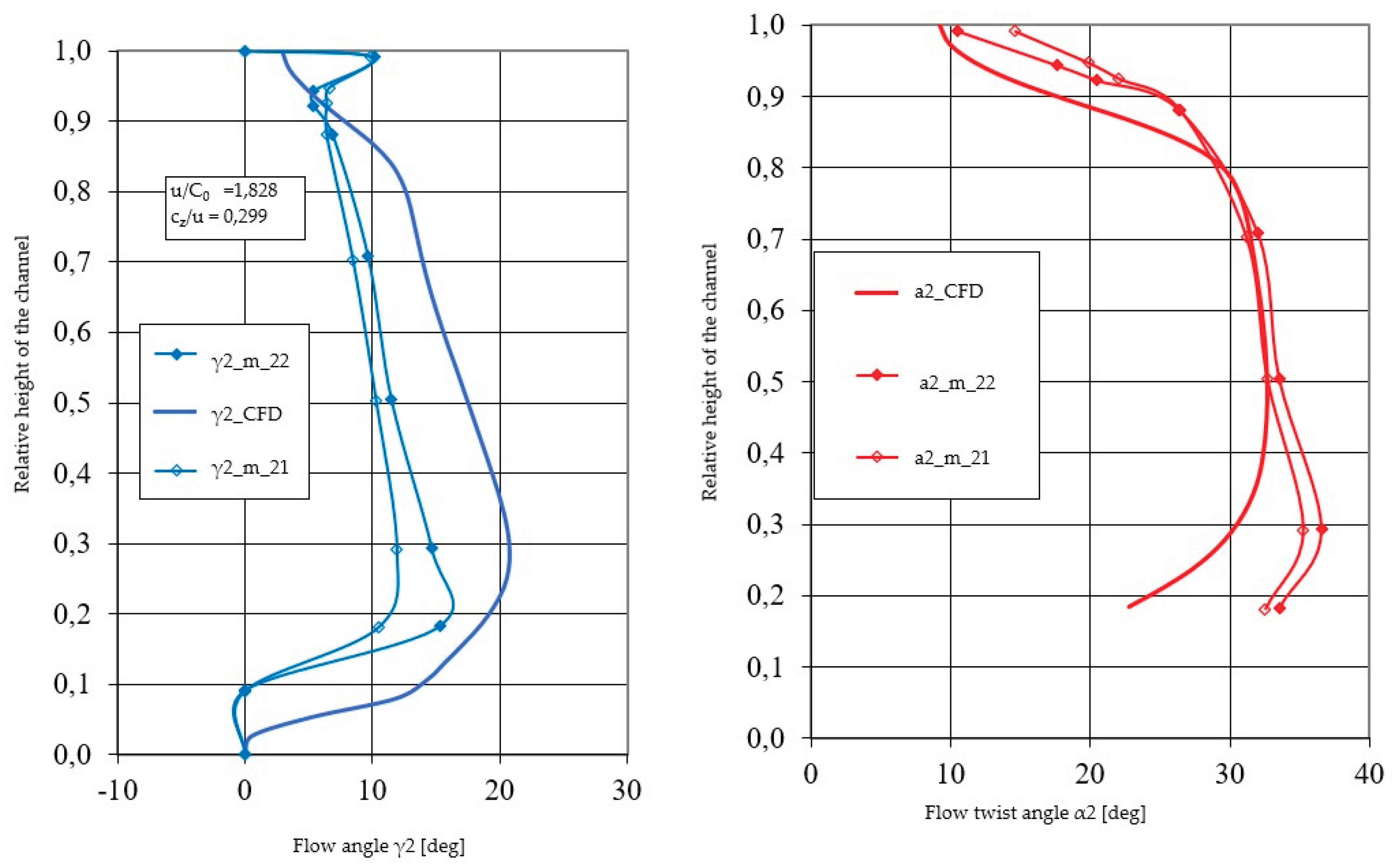
In order to give an understanding of the nomenclature of the figures above we give the following examples:
P2*m: total/brake pressure on the middle diameter in the cross section 2-2
u/c0: characteristic number of the flow
cz/u: the ratio of the “z “component (along the turbine axis) of the speed of the working medium to the tangential speed (u). Flow coefficient.
P2*_CFD_21: the total/brake pressure calculated through CFD for the first probe in the cross section 2-2
P2*_exp_22: the total/brake pressure measured during the experiment for the second probe in the cross section 2-2
Mr2_exp_21: The Mach number of the speed component perpendicular to the turbine axis (“r” direction) measured during the experiment (not CFD) from the first probe on cross section 2-2.
And so on. We want to remember that in cross section 2-2 we have two pneumometric probes situated diametrically opposite one from the other. Thus, the suffixes 21 and 22.
3.2. Calculation of the Additional Power Supply System (APSS)
The results of preliminary numerical modelling of the ‘S-D’ model system showed that at a rotor speed of n=11050 rpm in GTU idle mode, the power consumed by the model stage NMxGTU=11,900 kW. According to the results of the study of the the idle power of the last stage of the model compartment ‘S–D’ is NМхх4st=8,900 kW for the ET4 test bench. An electric motor was selected as the source of additional power. The rated speed of the electric motor shaft is 1500 rpm. To achieve the planned frequency, a multiplier with a transmission ratio of 8.613 and an electric current frequency regulator were included in the Additional Power Supply System (APSS).
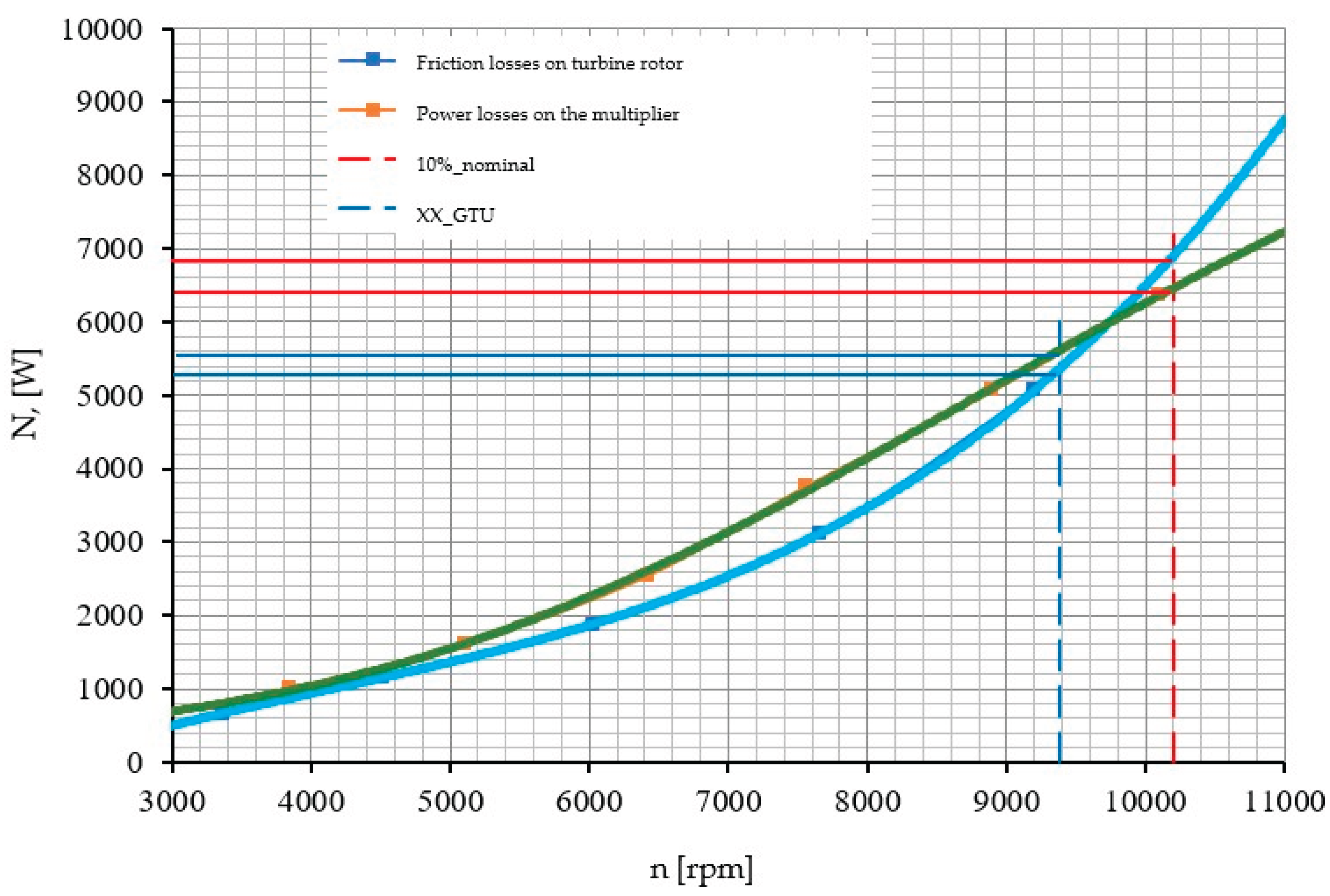
Power losses in the multiplier, according to experimental estimates, amounted to NMult ≈ 8.0 kW at an input shaft rotation speed of nin=1500 rpm (Figure 3.6).
Based on the above preliminary estimates, the required motor power was determined:
Nmotor= NMxGTU + NМхх4st + NMult >11.9+8.9+8≈ 30 kW
Figure 3.6.
Relationship between power losses in the multiplier and in the turbine rotor as a function of shaft speed.
Figure 3.6.
Relationship between power losses in the multiplier and in the turbine rotor as a function of shaft speed.
3.3. Test Programme for the High-Power Stationary Gas Turbine S-D System on the ET-4-XX Test Bench. Goals and Objectives
The main objective of this investigation is to work out the way for simulation of the idle mode of the last stage high power stationary GTU, when a2<a1 as was said in the introduction, which will allow to determine the characteristics of pulsation processes in the flow part of the ‘S-D’ system of the model in the specified extreme modes. Furthermore, this will allow us to obtain unique data on the key aerodynamic characteristics of the stage and the S-D system in a mode corresponding to the idle mode of a high-power stationary gas turbine.
Considering the above, the program for studying extreme partial load conditions, including the idle mode of a gas turbine, using the S-D system model will include several additional specialized experiments:
- Trial adjustment tests of the ‘S-D’ system in idle mode at various air flow rates in order to obtain experimental (real) dependencies: Nxx=f1(n) and Gxx=f2(n) and within the range of n = 0 ÷ 11000 rpm;
- Adjustment tests of the additional power supply system (APSS) to determine experimental dependencies Nelectrical motor= f3(n) U=f4(n) and I=f5(n) in the range n = 0 ÷ 11000 rpm. Here, “I” is the current in the electric motor, and “U” is the voltage of the electric motor;
- Control and commissioning tests of the ‘S – D’ + APSS system in the negative power mode of the model stage (n ≈ 11000 rpm);
- Standard tests of the ‘S–D’ + APSS’ system without additional air supply to the diffuser in the operating mode corresponding to the idle speed of the high power stationary GTU (n=10000 rpm,);
- Standard tests of the ‘S–D’ + APSS’ system with additional air supply to the diffuser in the operating mode corresponding to the idle speed of the high power stationary GTU (n=10000 rpm,).
3.4. Modified Test Bench ET-4-XX Test Bench for Experimental Modeling of the ‘S– D’ System in Idle Mode GTU.
In the gas turbine’s idle mode, the turbine’s last stage operates by absorbing the power generated by the first three stages. This mode cannot be achieved using the model block ‘S-D’, which includes only last stage, without additional power from an external source.
To achieve the gas turbine’s idle mode for model block ‘S-D’, the ET-4 experimental test bench should be upgraded with an additional power supply system (APSS). Figure 3.7 shows a photograph of the APSS of the upgraded ET-4-XX test bench.
Figure 3.7.
Additional Power Supply System (APSS) for experimental stand ЭТ-4-ХХ: 1 – frequency converter; 2 – electrical motor; 3 -multiplier; 4 – bracket; 5 – plastic coupling MUP-1-60; 6 – mounting plate for base unit; 7 –lubrication system for multiplier; 8 – cooling system for multiplier.
Figure 3.7.
Additional Power Supply System (APSS) for experimental stand ЭТ-4-ХХ: 1 – frequency converter; 2 – electrical motor; 3 -multiplier; 4 – bracket; 5 – plastic coupling MUP-1-60; 6 – mounting plate for base unit; 7 –lubrication system for multiplier; 8 – cooling system for multiplier.
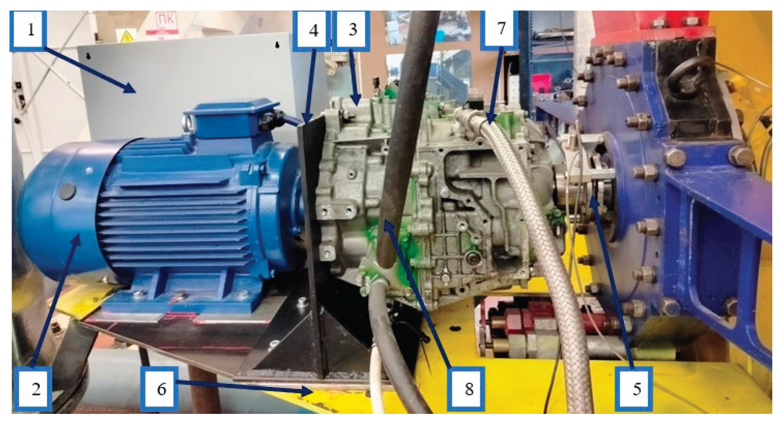
Multiplier 3 is a converted Toyota P410 engine gearbox. After complete overhaul, the multiplier has a transmission ratio of z = 8.613, an output shaft speed of 11,000 rpm, and a transmitted power of 40 kW. It is mounted on a specially manufactured high-rigidity bracket 4 using a vertical flange connection of the housing. The low-speed input shaft of the multiplier is connected to the electric motor shaft 2 by a special coupling. The output shaft of the multiplier is connected to the model stage rotor by a specially made plate coupling 5. The 5AI 180 M4 motor is controlled by a special device – a frequency converter 1, model ITD 373 U 4383. The frequency converter 1 allows the speed of the electric motor rotor to be varied within the range = 0 ÷ 1500 rpm. The rotation frequency of the multiplier output shaft varies within the range of 0÷11000 rpm.
The auxiliary power supply system (APSS) is designed as an extension of the ET-4-XX stand foundation frame to ensure the alignment of the turbine shaft and the new drive system. The mounting plate for base unit 6 consists of a 10 mm thick steel plate reinforced with a grid of channels to increase its rigidity, which are fastened to the underside of the plate with M10 bolts along each channel. The plate is laid on two corner brackets rigidly fixed to the foundation frame of the ET-4-XX stand and on two supports installed on the concrete foundation of the stand on the other side of the steel plate. The four-support system allows the mounting plate to be strictly leveled. This makes the base device a continuation of the ET-4-XX stand foundation, which ensures precise centering of the turbine and the new drive with an electric motor.
This design of the base mounting jig proved to be so effective that further shaft alignment was performed with an accuracy of 0.02 to 0.04 mm. This accuracy ensured full operability of the design up to a model stage shaft rotation speed of n = 11,000 rpm. At the same time, an intense increase in oil temperature was detected in the multiplier, reaching 135 ÷ 150 °C during the first hour of operation of the test bench. Therefore, water cooling of the multiplier was provided at the design. This reduced the oil temperature to 90 °C. The water connection was made from the already existing hydraulic brake system.
A longitudinal section of the ET-4-XX test bench is shown in Figure 3.8.
Figure 3.8.
Longitudinal section of the ET-4-XX test bench for experiments on idle mode regimes of high power stationary GTU.
Figure 3.8.
Longitudinal section of the ET-4-XX test bench for experiments on idle mode regimes of high power stationary GTU.
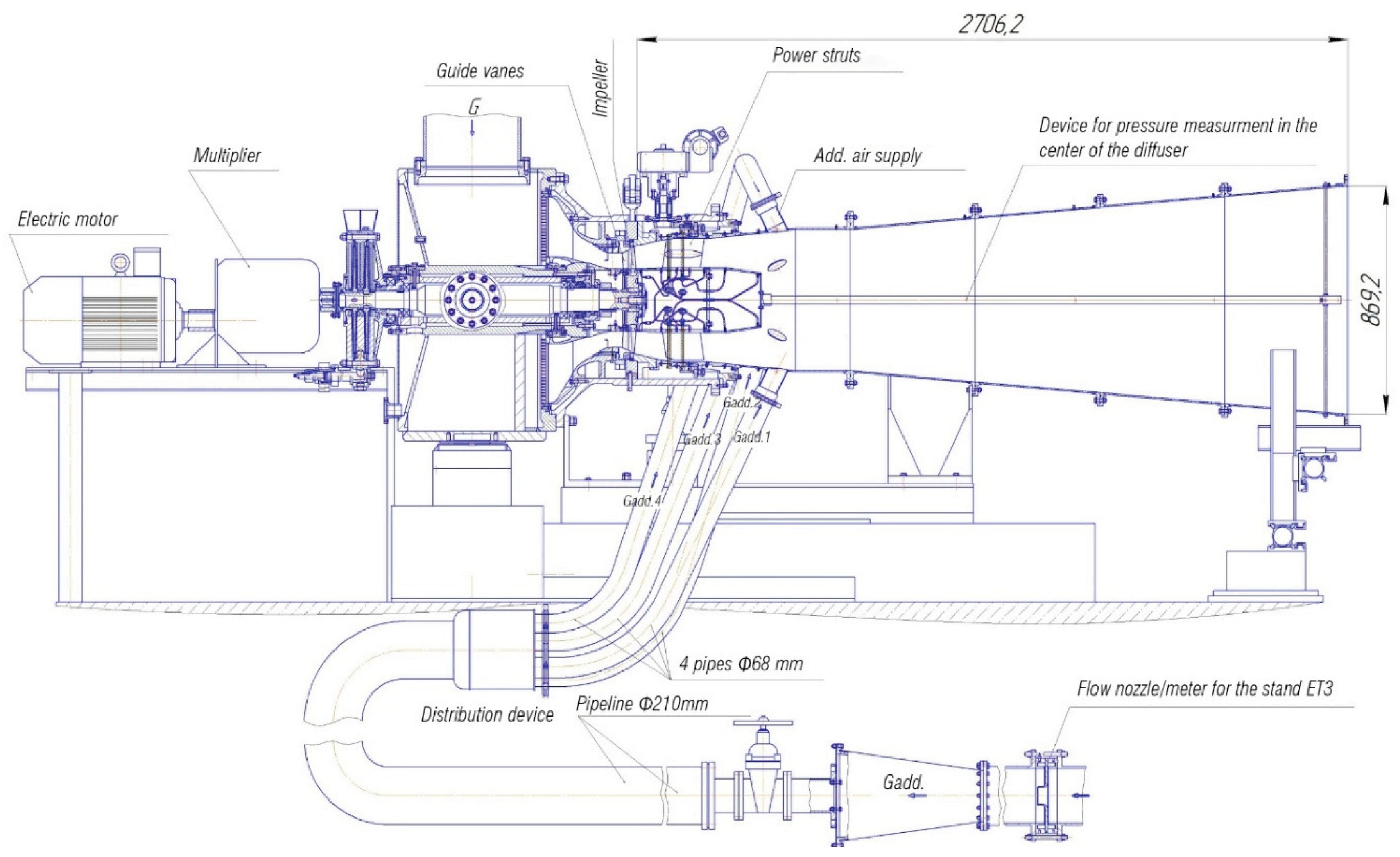
The aerodynamics of the ‘S – D’ system for specified partial load modes are simulated both with and without additional air supply to the diffuser. Additional air supply to the diffuser on the ET-4-XX model stand is provided by four pipes with a diameter of 68 mm at the diffuser inlet, with accurate modelling of the air supply in accordance with the scale of the entire ‘S-D’ system model, equal to 1:4.566 of the actual geometric dimensions.
In ventilation mode, the flow leaves the impeller with high swirl and with such swirl, the flow is displaced and concentrated in the peripheral sections of the diffuser. Under these conditions, the pressure measurement ports located at the periphery of the diffuser cannot characterize the average pressure in the corresponding cross-section of the diffuser flow path. Therefore, for these specific flow conditions, a special device was manufactured and installed to measure pressures in the center of the diffuser in the form of a fixed pipe Φ32 mm, in which receiving holes with fittings are made for each of the control sections of the diffuser.
The Φ4 mm hose branches are located behind the diffuser, in the low-velocity flow zone, through a special outlet. It should be noted that the technique used to measure pressures at the center of a highly swirling flow significantly increases the accuracy of the results averaging these pressures across the section under study, and with it the accuracy of the local pressure recovery coefficients in the diffuser Cp along its length at such extreme operating modes of the stage.
3.5. Methodology of Experimental Research in a Quasi-Stationary Setting
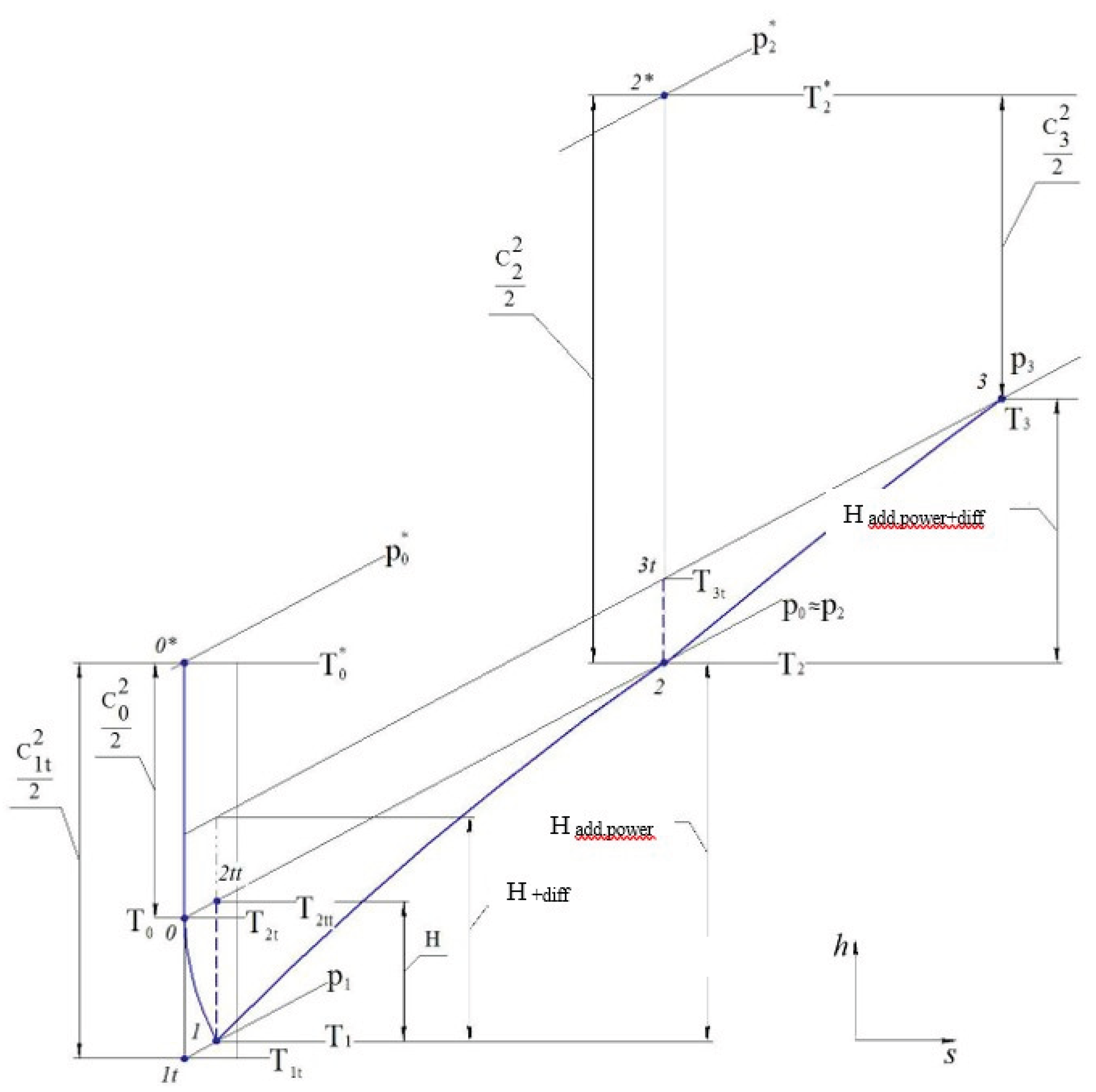
At load modes of 10% of rated power and idle speed of the high power stationary GTU, the last stage of the turbine operates with power absorption. The working process in the ‘S – D’ + APSS at these modes is schematically represented in Figure 3.9 in “h-s” coordinates.
This flow structure can only be achieved by supplying additional power to the impeller of the last stage of the turbine, which is transmitted through the rotor shaft from the first three stages. Thus, the impeller transfers mechanical energy to the flow moving through it. This process is represented in the “h-s” diagram by polytropic curve 1-2 and isentropic curve 2-2*. Consequently, the additional energy supplied is spent on increasing the pressure from p1 to p2 (process 1-2) and on the kinetic energy behind the impeller (process 2-2*). The final conversion of energy in the mode under consideration occurs along polytropic 2-3.
Figure 3.9.
Work process in the ‘S – D’+APSS system in idle mode of a single-shaft gas turbine.
3.6. Mathematical Apparatus for Processing Experimental Data
Representing the operating process in a turbine stage with additional power input facilitates a deeper understanding of energy generation and absorption processes. Based on the hs-diagram, a mathematical framework was developed for processing experimental data and calculating the integral characteristics of the stage and the ‘S-D’ block, taking into account the additional power input.
Additional power transmitted to the shaft from the APSS:
where Nelec.motor - power consumed by the APSS electric motor, [W]; Nmult- power lost in the multiplier, [W].
The power delivered to the flow by the impeller compressing the flow in the modes under study is determined by the additional power supplied minus the power lost in the bearings Nb. The enthalpy drop that takes place by the compression process in the impeller is determined by the formula:
Here, “G” is the mass air flow through the model stage in kg/s.
The useful enthalpy increase of the compression process from point 1 to point 2 is determined by the temperature difference in the flow in sections 1-1 and 2-2:
Taking into account formulas (3.1) and (3.2), the efficiency of the stage is equal to:
The enthalpy difference recovered in the diffuser in an ideal process is equal to:
The actual enthalpy difference recovered in the diffuser is equal to:
According to the h-s diagram in Figure 3.10, the useful enthalpy difference in the system Last Stage-Diffuser ‘S - D’ is equal to:
The enthalpy consumed is equal to:
Taking into account formulas (3.9) and (3.10), the efficiency of the Last Stage-Diffuser ‘S - D’ system is equal to:
4. Discussions
4.1. Results of the Numerical Flow Simulation
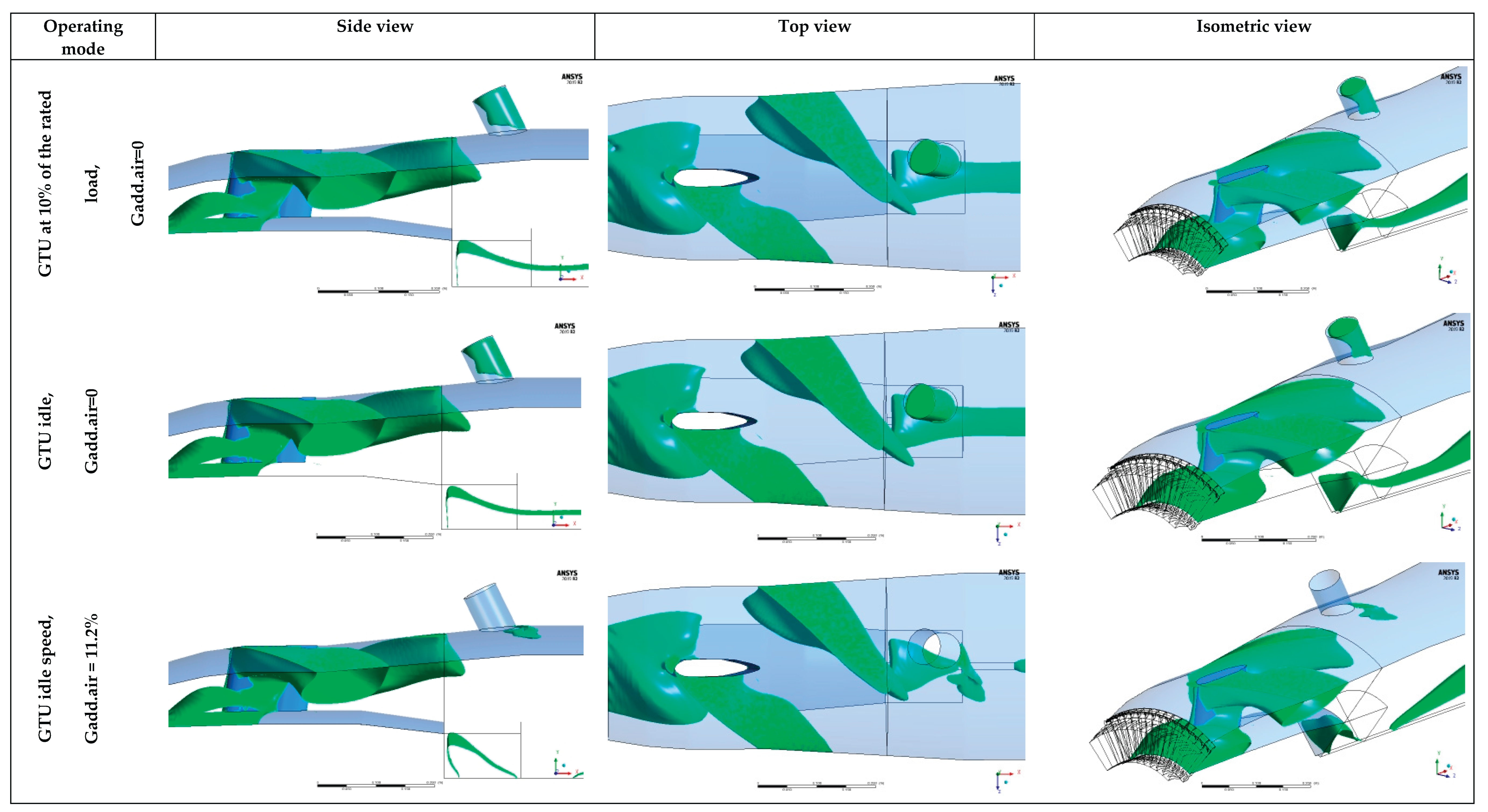
The results of the numerical simulation of the flow under the specified load conditions are presented in Figure 4.1–4.3 in the form of streamlines and separation zones in the annular diffuser. Numerical modeling of extreme partial regimes for the model flow was performed using DES approach to take into account additional losses caused by the significant non-stationary nature of the flow in the annular diffuser. The streamlines in Figure 4.1 indicate that the vortex separation zone in the diffuser is concentrated in its annular section. The location of the vortex zones can be seen in more detail in Figure 4.2, which shows the streamlines in the inter strut space of the annular diffuser. Figure 4.2 (side view) clearly shows the return flow region in the inlet section of the annular flow immediately behind the impeller. The transit flow is concentrated in the upper part of the diffuser and impinges on the power strut almost perpendicularly (top view, Figure 4.2). This allows us to expect significant pressure pulsations on the hub surface in the inter strut space and on the strut surface on the side opposite the incoming flow.
Furthermore, pulsations can be expected at the end of the hub due to the vortex structure from the adjacent support strut (Figure 4.2, top view).
This is also confirmed by Figure 4.3, which shows areas of separated return flows.
Figure 4.1.
Streamlines in the outlet diffuser at extreme partial load conditions.
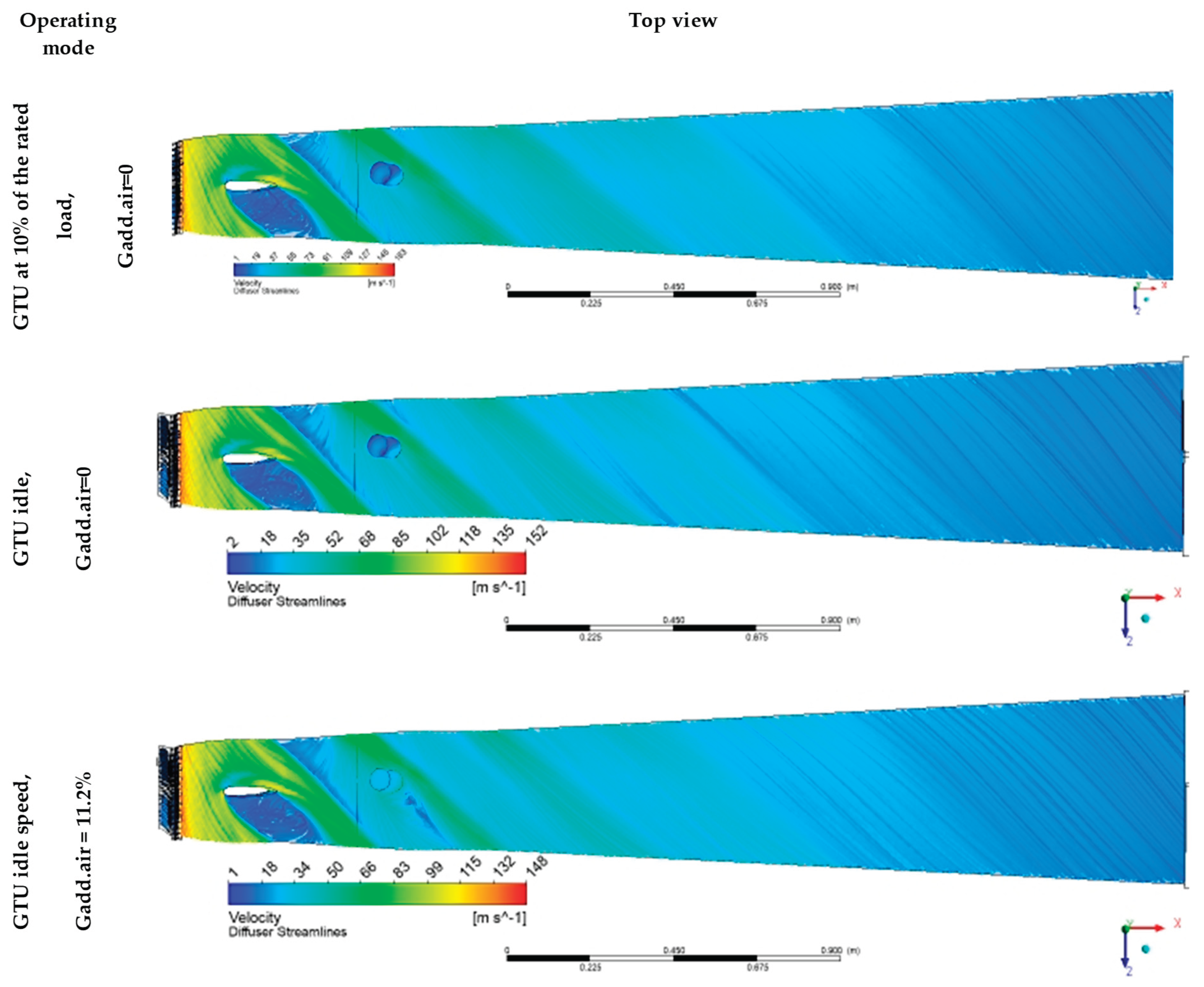
Figure 4.2.
Flow lines in the inter-column space of the annular part of the outlet diffuser at extreme partial load conditions.
Figure 4.2.
Flow lines in the inter-column space of the annular part of the outlet diffuser at extreme partial load conditions.
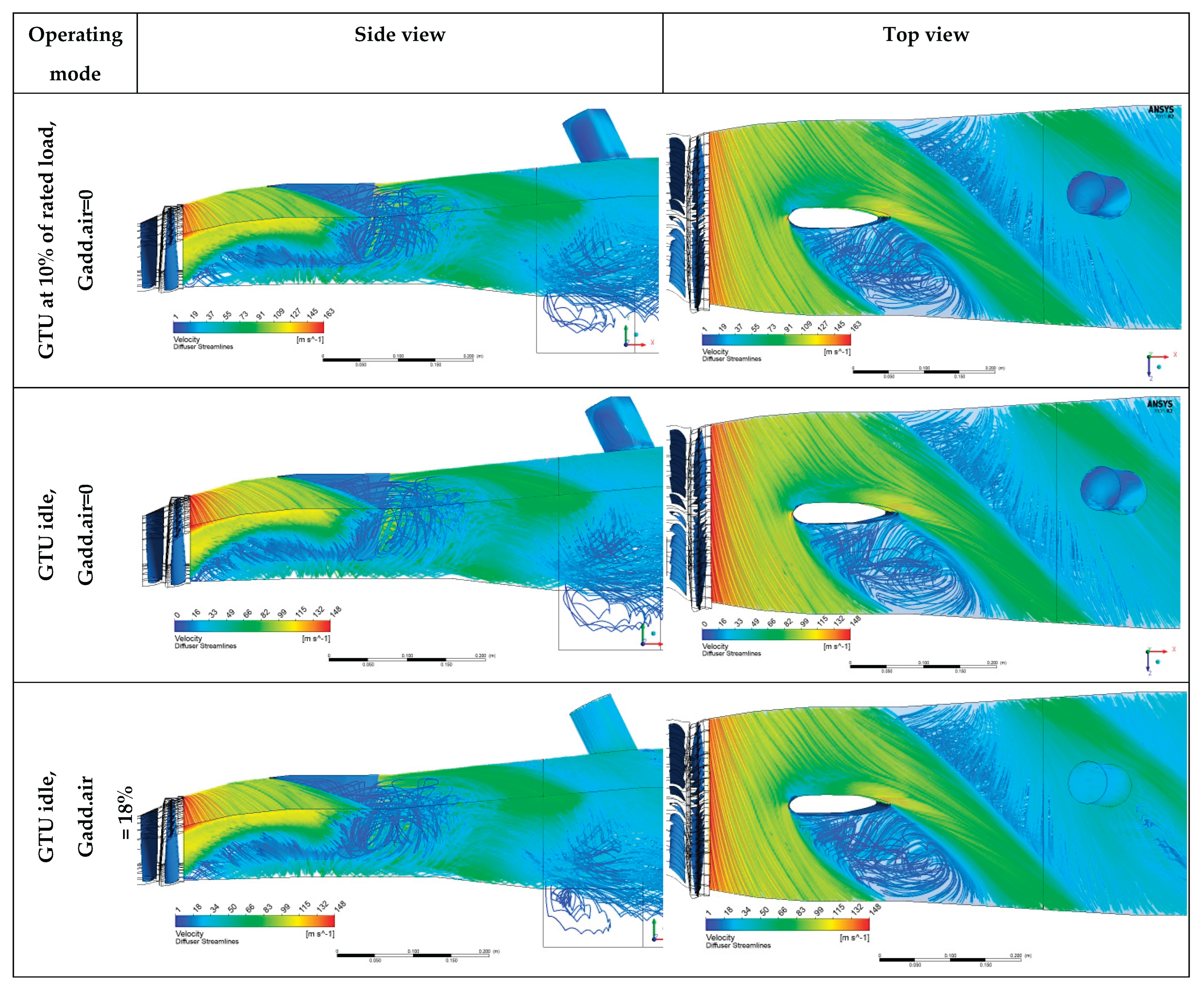
Figure 4.3.
Flow separation patterns in the diffuser at 10% of rated load and at gas turbine idle.
4.2. Unsteady Characteristics Measuring System
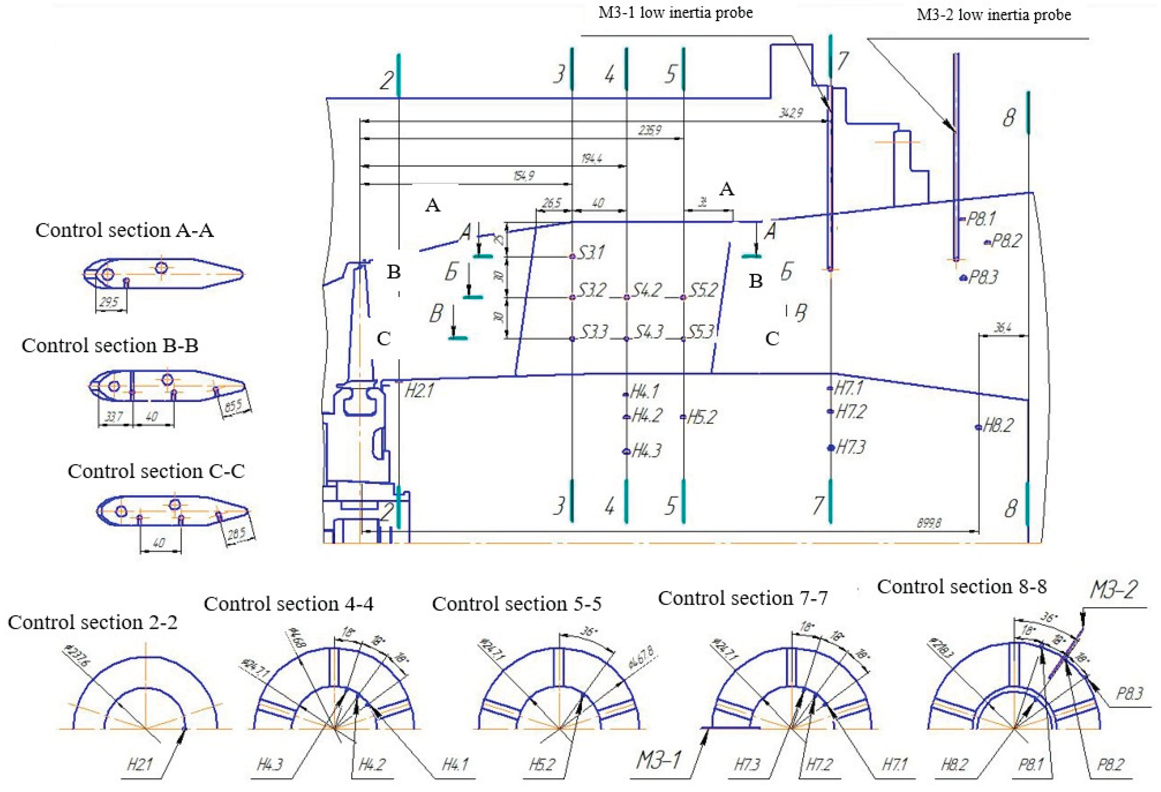
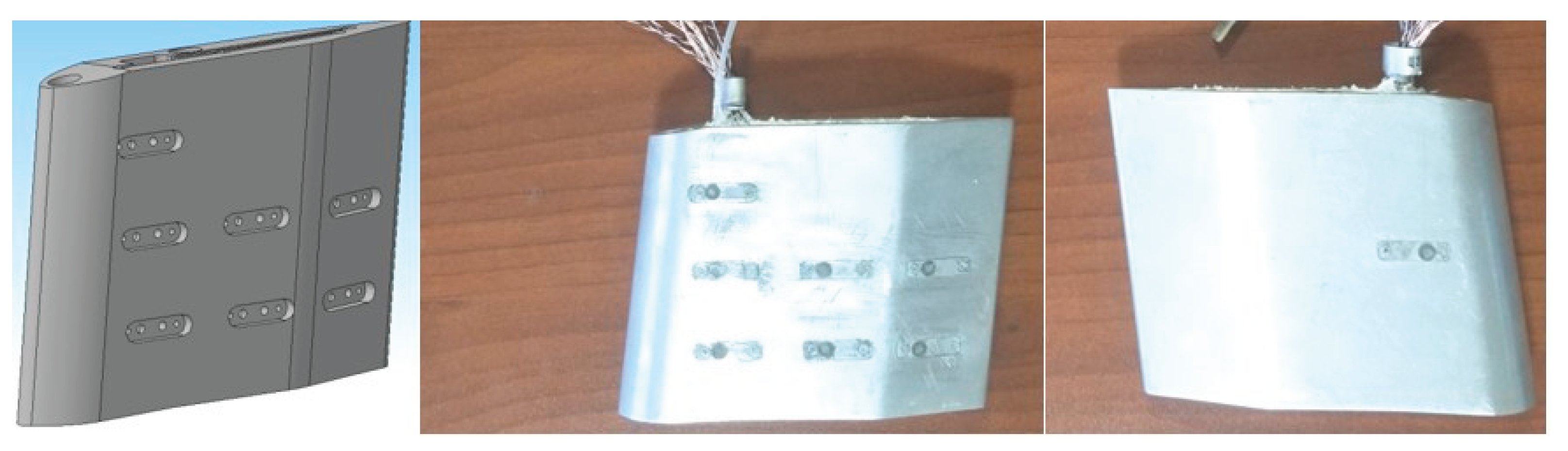
From the flow patterns (streamline in ANSYS CFX) and the 3D flow separation graphics, we can now conclude about the positioning of the sensors for the measurement of the pressure pulsations during idle state of the GTU. The system for measuring non-stationary flow characteristics is designed to determine these pressure pulsations “δP” in the flow behind the power struts, on the surfaces of the power struts and the diffuser sleeve. The sensor layout was determined based on the results of numerical modelling of 10% rated power modes and GTU idle mode and low-inertia pressure sensors that register wall (static) pressure pulsations should be installed flush with the surfaces of the power struts, hubs, and peripheral circuit. The sensor designations correspond to their position on the strut (S), hub (H) or periphery (P) and the number of the measuring section. Low-inertia probes are placed in coordinate systems to record full pressure pulsations “δP*” behind the strut in measuring sections 6-6 and 8-8.
The results of numerical modeling of extreme partial flow conditions also suggested the presence of velocity pulsations in the diffuser inlet section, which would cause total pressure pulsations in the section downstream of the impeller. Therefore, it would be advisable to supplement the system for measuring transient processes in the diffuser with a low-inertia total pressure sensor.
A transient calculation using the DES approach allowed for a preliminary assessment of the frequencies and amplitudes of the total and static pressure pulsations in the study area. Based on this assessment, signal synchronization and amplification units were chosen for the measurement system.
Thus, the pressure pulsation measurement diagram should be included low-inertia pressure sensors installed on the surface of the H sleeve, S struts, and peripheral surface P of the diffuser, as well as a low-inertia MZ probe, a rotation sensor, multichannel amplifiers, and analog-to-digital converters (ADCs) connected via a USB interface to computers, as well as a digital oscilloscope.
The PowerGraph 3.3 software package from DISoft LLC is used to control the data acquisition and processing modules. The software package records data transmitted from the ADC, digitally calibrates, filters, and visualizes it in real time during the experiment. Further analysis of the results is performed offline using built-in statistical and spectral processing subroutines.
The measurement diagram of pressure pulsation measurements in the flow and on the surfaces of the annular diffuser is shown in Figure 4.4. The measurement system provides parallel multi-channel recording of signals from low-inertia sensors in a frequency band of at least 20 kHz in arrays of 8 channels.
Figure 4.4.
Schematic diagram of pressure pulsation measurements in the flow and on the surfaces of the annular diffuser.
Figure 4.4.
Schematic diagram of pressure pulsation measurements in the flow and on the surfaces of the annular diffuser.
4.3. Measuring Devices and Measuring Equipment for Recording Flow Unsteady Characteristics.
To determine the parameters of the pulsation components of the flow in the flow section of the studied model system ‘S–D’ high power stationary GTU, as it was mentioned, a low-inertia pressure (LIP) probe was chosen. The (LIP) probe should be installed at a specified point in the flow section using a coordinate device (see the measurement diagram in Figure 2.5 and 2.6). The sensors are based on identical MPX pressure sensors manufactured by Motorola (USA). The MPX2300 sensor is a miniature piezoresistive pressure sensor. The sensor contains a sensitive element made of single-crystal silicon with strain gauges integrated into the membrane body. The necessary metrological characteristics are ensured by built-in temperature compensation and calibration circuits.
Pressure sensor characteristics:
- Measurable pressure range: 0–40 kPa.
- Pressure compensation level: up to 40 kPa.
- Time constant: 1 ms.
- Output signal in the range: 10 mV/5 V.
- Relative error: +/-5%.
- Operating temperature range: from +10 °C to +80 °C.
The H and S sensors installed on the surface of the bushing and struts are shown on the Figure 4.5 and 4.6).[11]
Figure 4.5.
Design of a ring/sleeve diffuser with low-inertia pressure sensors of type H.
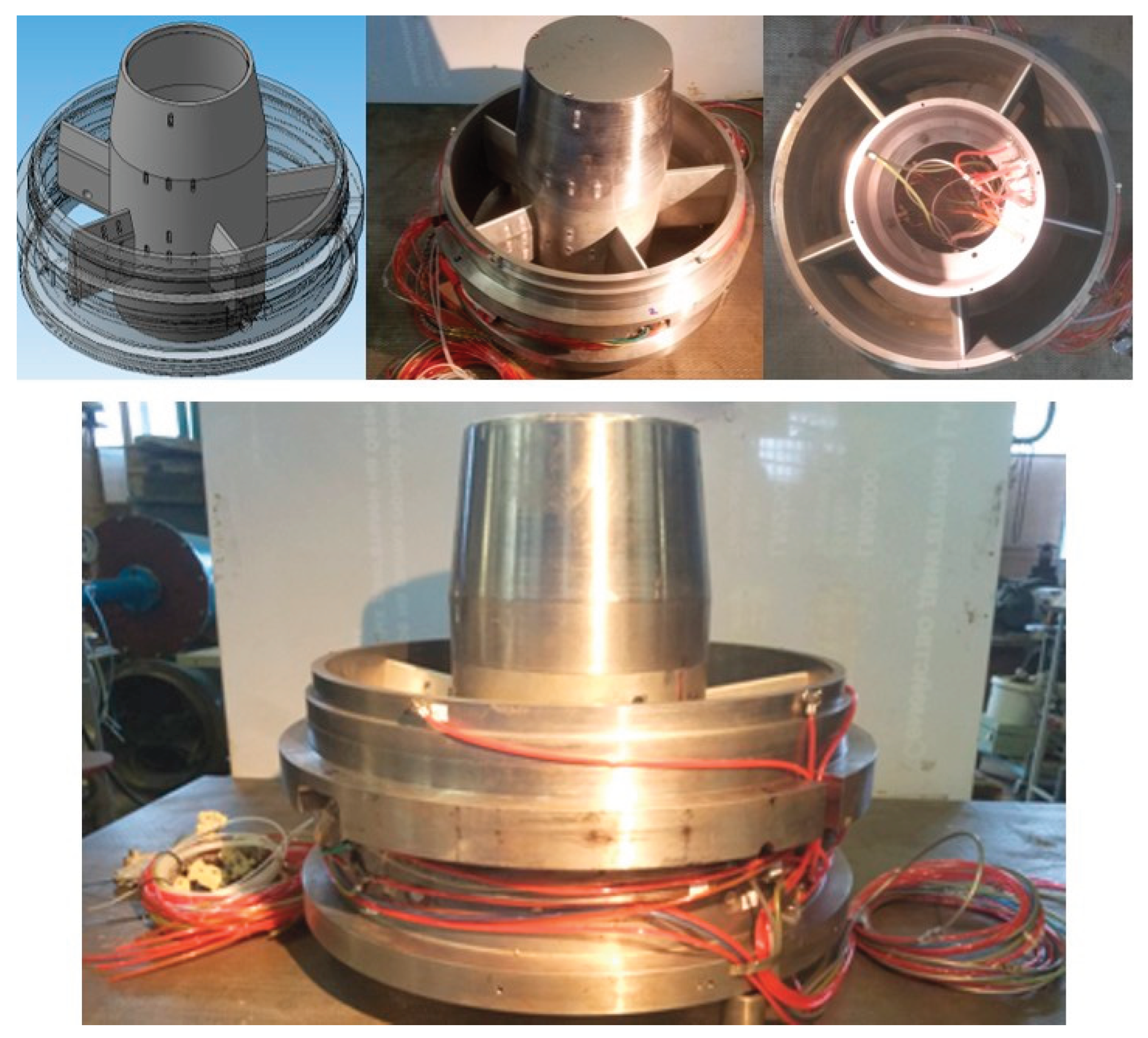
Figure 4.6.
Power struts with built-in low-inertia pressure sensors, type S.
5. Conclusions
With the new measurement scheme of the ET4 test bench now equipped with the low inertia pressure sensors on the power struts and the sleeve as well as the APSS unit as an external source of power, we can now proceed to an experiment for the mapping of the pressure pulsations in the area of the struts and the exit of the last stage. This way we will be able to measure the frequencies which are formulated in such extreme partial modes and from discreet values of pressure pulsation measurement, we can obtain a continuous function through extrapolation about the pulsation of the static pressure in all the area at the exit of the last stage and into the diffuser. This can lead us to check for the reliability [13] of the whole unit under circumstances of extreme partial working regimes [14] or idle mode of the turbine.
Nomenclature
The following symbols are used in the manuscript:
c absolute velocity [m/s]
h enthalpy [kJ/ (kg · K)]
n rotor speed [rpm]
H total enthalpy [kJ/ (kg · K)]
P* total pressure [Pa]
T* total temperature [K]
u tangential velocity [m/s]
R gas constant [Joules/kg К]
k isentropic exponent
ω angular velocity [rad/sec]
M2 Mach number in section 2-2
G mass flow rate [kg/sec]
Re2 Reynolds number in section 2-2
u/C0 characteristic number
cz/u flow coefficient
М torque N·m;
G mass flow kg/s;
H0+dif isentropic enthalpy drop from the total parameters in the inlet of ‘S-D’ system to the pressure in the flow behind diffuser, in section 13-13 J/kg;
H*0+dif isentropic enthalpy drop from the total parameters p*0, T*0 in the inlet of the ‘S-D’ system to the total parameters behind diffuser, in section 13-13 J/kg.
η stage efficiency
η* efficiency measured according to total parameters
η+diff total efficiency of the S-D system
H0 isentropic enthalpy drop from the total parameters in the inlet of ‘S-D’ system to the pressure in the flow behind step, in section 2-2 J/kg;
H*0 - isentropic enthalpy drop from the total parameters in the inlet of ‘S-D’ system to the pressure in the flow behind step, in section 2-2 J/kg.
Cp pressure recovery coefficient in the diffuser
α2m exit angle from the impeller on the middle diameter [deg]
ρт thermodynamic reactivity index
ρк kinematic reactivity index
Sh Strouhal’s number
Fr Froude number
cu circulation coefficient
cz flow coefficient
N power [kW]
δP static pressure pulsations
Abbreviations
The following abbreviations are used in this manuscript:
CFD Computational fluid dynamics
RANS Reynolds-averaged Navier-Stokes
DES Detached Eddy Simulation
APSS additional power supply system
References
- Kirillov, Alexander Ivanovich; Galaev, Sergey Alexandrovich; Isupov, Vasily Yuryevich; Smirnov, Evgeny Mikhailovich. Application of vortex-resolving methods to the calculation of three-dimensional flow in a gas turbine outlet diffuser. Sci.> Tech. Bull. St. Petersburg State Polytech. Univ. 2014, No. 4(207), 16–25. [Google Scholar]
- Borishansky, K.N.; Borishansky, K.N. Vibrations of steam turbine blades and measures to combat them; Art-Xpress: St Petersburg, 2011; p. 324. [Google Scholar]
- Cherkasova, M.G.; Semakina, E. Yu; Chernikov, V.A. Validation of a numerical method for studying the ‘Stage-Diffuser’ system and its application to design upgrades. J. Samara Univ. Aerosp. Eng. Technol. Mech. Eng. 2022, Vol. 21, 38–47. [Google Scholar] [CrossRef]
- Semakina, E. Yu.; Chernikov, V. A.; Sukhanov, A. I. Pressure pulsations in the flow and vibration of gas turbine engine exhaust components. Sci. Tech. Bull. St. Petersburg Polytech. Univ. Nat. Eng. Sci. Vol. 23(No. 2.), 28–40. [PubMed]
- Fedyakov, E. M.; Koltakov, V. K.; Bogdatyev, E. E. Measurement of Variable Pressures. Mosc. Stand. Publ. House 1982, 216. [Google Scholar]
- 6. Chernikov V.A., Experimental stand for turbines exhaust diffusers and inlets gas-dynamic analyses. In Heat-Power Engineering; 2008; Volume №6, pp. 49–54.
- 7. Lapshin K.L, The theory for optimal design for thermal turbomachines. In Lecture notes; pp(37,38) Ministry of education and science of the Russian Federation, Federal state autonomous educational institution for higher education-Saint Petersburg, Polytechnic University “Peter the Great”: Saint Petersburg, 2018.
- Chernikov, V.A.; Yu, Semakina E. Information-computational System of Aerodynamic Stand for stream study in flow path of “stage-diffuser” section and some testing results on heavy-duty gas turbine model. In Energy converting machinery and units; 2008; Volume № 1, pp. 24–34. [Google Scholar]
- Mimic, D.; Drechsel, B.; Herbst, F. “Correlation between Pressure Recovery of Highly Loaded Annular Diffusers and Integral Stage Design Parameters”. Proceedings of ASME Turbo Expo 2017, Turbomachinery Technical Conference and Exposition, Charlotte, USA, 2017. pp. GT2017–63586. [Google Scholar]
- ANSYS CFX User’s Guide. 2023.
- The Current State of Hydrodynamics of Viscous Fluids / Ed. by S. Goldstein. Moscow: IL, Vol. 2. pp. (96, 98), (248), (408). 1948.
- 9000 Series Intelligent Pressure Scanners User’s Manual – Pressure Systems, Inc.
- Borishansky, K.N. Types of self-oscillations in steam turbine blades and measures to combat them. Scientific and Technical Bulletin of St Petersburg State Polytechnic University. St Petersburg. No.2. (171) (pp. 52–60) 2013.
- Sukhanov A.I, “Aerodynamic Excitation of Turbine Blade Vibrations in a Compressible, Transient Flow and Improvement of the Method for Calculating Variable Loads”, Dissertation for the Degree of Candidate of Technical Sciences, Leningrad, 1984.
Disclaimer/Publisher’s Note: The statements, opinions and data contained in all publications are solely those of the individual author(s) and contributor(s) and not of MDPI and/or the editor(s). MDPI and/or the editor(s) disclaim responsibility for any injury to people or property resulting from any ideas, methods, instructions or products referred to in the content. |
© 2026 by the authors. Licensee MDPI, Basel, Switzerland. This article is an open access article distributed under the terms and conditions of the Creative Commons Attribution (CC BY) license (http://creativecommons.org/licenses/by/4.0/).
Copyright: This open access article is published under a Creative Commons CC BY 4.0 license, which permit the free download, distribution, and reuse, provided that the author and preprint are cited in any reuse.


