

Submitted:
15 July 2026
Posted:
16 July 2026
You are already at the latest version
Abstract
Monitoring the current technical condition of a marine internal combustion engine and diagnosing the causes of deviations of its operating parameters from reference values are important tasks for ensuring the efficient and safe operation of marine power plants and vessels in general. This paper investigates the theoretical founda-tions, methods, and practical implementation of a digital twin of a marine internal combustion engine as a tool for solving these tasks. The main requirements and stages of digital twin development are presented, including: calibration of the mathematical model; determination of the set of sensors and other input data obtained from the op-erating engine; identification of the current engine operating mode; definition of objec-tive functions characterizing deviations of engine operation from reference conditions; and automation of fault detection algorithms. In particular, modifications introduced into the mathematical model of engine operating processes are presented, allowing more flexible representation of fuel injection characteristics as well as automatic ad-justment of model parameters according to the identified engine operating mode. A fault detection method based on simulation modeling and the classical theory of design of experiments is proposed. The four-factor fractional factorial experiments were per-formed, followed by analysis of the obtained results using second-order polynomial regression equations. The results demonstrate that the proposed method provides cor-rect identification of engine faults, although the numerical values of the investigated factors are determined with a certain error. Therefore, further development of the proposed approach requires improvement of the mathematical model, formulation of explicit rules for selecting the investigated factors, and automation of fault identifica-tion methods under conditions of cycle-to-cycle variability of the engine working pro-cess and measurement uncertainties.
Keywords:
technical condition diagnostics
; marine internal combustion engine
; digital twin
; design of experiments
; objective function
; condition monitoring
1. Introduction
Internal combustion engines (ICE) are key components of a ship power plant, and their reliable operation directly affects the economic efficiency of vessel operation, navigation safety, and the level of environmental impact. Therefore, continuous efforts are being devoted to improving engine design, optimizing engine working processes and operational methods [1], as well as adapting engines to new fuels and regulatory requirements [2].
One of the major directions contributing to the improvement of marine ICE operation efficiency is the implementation of modern digital technologies for continuous technical condition monitoring, automation of engine control, and development of onboard self-diagnostic systems capable of assessing the current engine condition during operation. The development of this field has led to the emergence and practical implementation of digital twin (DT) technologies [3,4].
Manufacturers of modern marine engines already offer commercial services based on DT technologies. Everllence provides the PrimeServ Assist platform for real-time monitoring and AI-based diagnostics [5]. Wärtsilä offers the Operational Performance Improvement & Monitoring (Operim) system, which integrates a virtual twin for comparison between actual and expected engine performance [6]. WinGD developed the WinGD Integrated Digital Expert (WiDE) platform , which utilizes a customized DT model based on factory test data to provide actionable engine health assessment [7,8]. Nevertheless, further improvement of this technology remains an important research task.
A digital twin can be defined as a virtual representation of an internal combustion engine that reproduces selected aspects of its operation and behavior. Depending on its intended purpose, a DT should provide the most reliable possible prediction of variations in engine and subsystem parameters under different operating conditions. Digital twins of ICE may serve different purposes and can be classified as follows.
By purpose:
- engine control;
- engine diagnostics and condition monitoring;
- engine repair and maintenance;
- engine design and optimization;
- personnel training and teaching;
By primary focus:
- engine operating process;
- wear, lubrication, and cooling processes;
- thermal and mechanical stresses;
- engine component design and assembly.
By deployment architecture:
- embedded into the engine ECU;
- remotely accessible cloud-based systems;
- standalone PC-based installations.
Digital twins have a potential of application during the whole engine lifecycle, starting from its design and production [9]. The most challenging task in terms of achieving both high computational speed and high prediction accuracy is the development of DT intended for real-time engine control [10]. Such DTs may operate as “shadow models” running in parallel with real ECUs to validate control actions or predict engine behavior before actual actuation. DT could be an effective and cost-saving instrument for educational and training purposes [11].
However, the most widespread application of digital twins for marine ICE is technical condition diagnostics and condition monitoring. Intensive research efforts in this area are aimed both at improving mathematical models specifically adapted for DT applications [12,13] and at enhancing interaction between the digital twin and the real engine through sensor systems [14], including integration into comprehensive ship power plant diagnostic systems [15,16]. Particular attention should also be paid to the growing application of machine learning techniques in systems employing digital twins [17,18,19,20,21].
Despite the significant progress achieved in this field, the effective application of DT for diagnostics and condition monitoring of marine ICE still requires overcoming several important challenges. First, it is necessary to ensure an appropriate balance between the level of detail of the DT mathematical model and computational speed, especially for online monitoring applications or when diagnostic conclusions must be obtained during real-time engine operation [22]. Second, reliable identification of the current engine operating mode by the digital twin must be ensured, which requires determination of the necessary sensor set and appropriate methods for sensor data processing [23]. Finally, robust methods for fault identification and technical condition assessment using digital twins should be developed to ensure acceptable diagnostic reliability, support automation, and provide unambiguous diagnostic conclusions.
2. Definitions
Although the application of mathematical modeling to the diagnosis of the technical condition of ICE is a widespread practice, the theoretical foundations and methodological approaches to the application of DT for technical condition diagnostics remain insufficiently systematized. In particular, the application of DT for representing engine working processes requires the development of algorithms for automated simulation and extraction of diagnostic features capable of indicating deviations in engine technical condition.
Consider several definitions. An engine operating mode is defined as the set of operational engine parameters that characterize the current load and control state of the engine without considering its technical degradation. An engine possesses a set of operating modes , while each individual operating mode belongs to this set:
A technical condition of the engine is defined as the set of parameters describing the technical properties and degradation state of the engine and its subsystems. For the set of technical conditions , each particular technical condition is considered as:
The reference technical condition is defined as the factory condition of the engine or as its optimal technical condition.
Monitoring of the engine working process is defined as the observation, analysis, and statistical processing of a set of measurable engine parameters under given operating conditions. For the space of observable parameters , a particular available vector of the monitored parameter may be denoted as :
Figure 1 shows schematically the interaction of vectors , and as constituents of their sets for a given engine under given conditions of operation. While some of the parameters are common for all three vectors, another are specific for each.
The mathematical model of an engine working processes may be represented in the following general form:
where, the resulting vector is a function of the input parameter vector , the calculation control vector , the engine operating mode vector , and the technical condition vector .
The vector contains the simulation results, including engine working process parameters and corresponding process diagrams. The vector represents the input data used for calculations. This vector may be divided into two components: the vector of constant parameters , which remains unchanged between calculations for a given digital twin application scenario, and the vector of variable parameters , whose values change depending on the engine operating mode:
the constant parameters may include, for example, the geometric dimensions of the cylinder–piston group, the number of cylinders, and fuel injector characteristics. It should be noted that the set of constant parameters is specific to each engine and depends on the particular digital twin application scenario. The most commonly used variable parameters include crankshaft rotational speed, fuel injection timing, injection duration, boost pressure, and similar operating variables.
The vector may also be divided into two components: parameters available from sensor measurements and parameters that remain unknown due to the absence of corresponding sensors or the impossibility of direct measurement. Determination of the latter component represents a significant challenge and may influence the selection and configuration of the vector .
The vector may be interpreted as a set of parameters defining the calculation strategy or computational mode. For example, calculations may be performed with balancing of turbine and compressor power within the turbocharging system and determination of boost pressure, or alternatively with prescribed boost pressure values. Similarly, calculations may involve determination of the fuel injection timing required to achieve a specified maximum cylinder pressure, or may be carried out with fixed injection timing values.
3. Digital Twin Framework
According to the conceptual diagram presented in Figure 2, the application of a DT for diagnostics issues involves several functional stages:
- Calibration of the mathematical model of the DT for a particular engine using available experimental and documentation data.
- Determination of the sensor set through which the DT receives information about the current engine operating mode and its parameters.
- Determination of objective and constraint parameters, as well as parameters carrying diagnostic information regarding the engine technical condition.
- Definition of fault types and the corresponding healthy technical condition of the engine.
Therefore, calibration of the mathematical model for a digital twin involves not only performing simulations, but also comparing the obtained results with documentation and experimental data. Such comparison is performed for a subset of analyzed operating modes:
For each operating mode , a discrepancy vector is determined:
in this formulation, the vector may be interpreted as a vector of relative deviations between the simulation results and the available literature or experimental data.
The calibration process of the mathematical model may therefore be represented as an optimization problem aimed at minimizing the following functional:
An important stage in the application of a DT is identification of the current engine operating mode using the available (often highly limited) data obtained from sensors installed on the engine. These data may be represented by the observation vector . For this reason, preliminary calibration and tuning of the mathematical model are essential. The process of engine operating mode identification may also be represented as the following optimization problem:
The application of a DT for diagnostic purposes must solve the principal problem not merely of performing parallel simulation of engine working processes during diagnostic analysis, but also of developing algorithms capable of producing additional diagnostic criteria or indicators characterizing the technical condition of the engine. This may be formulated as determination of the engine technical condition deviation vector , which contains deviations between a selected set of characteristic engine parameters and their corresponding reference (desired) values:
importantly, the values of the vectors and may be obtained either experimentally, through simulation, or by a combination of both approaches, which introduces additional variability into digital twin applications.
From this perspective, minimization of the vector may be considered a formal representation of the diagnostic fault identification process, particularly when a set of parameters used for such minimization can be specified:
It may therefore be stated that the vector activates specific DT algorithms aimed at reliable identification of a particular fault.
Thus, the operation of a marine engine DT may be formally represented as an optimization problem whose solution consists in identifying the factors (parameters governing engine operation) responsible for the actual deviation of engine operating parameters from their reference or expected values. Analysis of these parameters and their values constitutes the diagnostic feature indicating a particular fault condition.
The development of effective methods and algorithms for solving this optimization problem therefore remains an important research problem.
3. Configuring the Digital Twin
Thus, the application of digital twins for solving problems related to diagnostics of the technical condition of internal combustion engines may be implemented according to different schemes and principles. One possible approach is considered below using the example of the laboratory test bench of Odesa National Maritime University based on a Weichai WP4 marine diesel-generator [25]. The core of the DT is based on the on-line service Blitz-PRO, which provides simulations of static and transient ICE operations with 0D-1D thermodynamic model [26,27].
According to the scheme presented in Figure 2, the main stages include calibration of the digital twin mathematical model, identification of the current engine operating mode, and diagnostics of the engine technical condition.
Mathematical Model Calibration
At the first stage, calibration of the mathematical model is performed considering the operating mode space . For the investigated engine, this space is limited to certain regions around fixed engine operating modes, as shown in Table 1.
To determine the mathematical model calibration parameters, i.e., to obtain the array of vector values , both literature data and experimental engine test data were used. Such experiments should preferably be carried out according to classical experimental procedures, namely:
- ensuring steady-state engine operation with stabilization of all controlled parameters, primarily temperatures of cooling media and exhaust gases;
- applying averaging procedures over a sample of 50–100 consecutive engine cycles in order to reduce the influence of cycle-to-cycle variability of the engine working process.
Obviously, such experiments require specialized equipment and laboratory test bench conditions; however, they provide the most reliable information regarding engine working processes. Table 2 and Figure 3 present examples of experimental data obtained in accordance with the above-mentioned principles.
A separate important problem is the processing of experimental data, during which several tasks must be solved:
- reliable determination of the top dead center (TDC) position;
- accounting for the influence of crankshaft angular velocity irregularity;
- averaging of sequential cycle data;
- determination of fuel injection timing and injection duration;
- determination of fuel ignition timing;
- calculation of fuel injection characteristics and heat release characteristics.
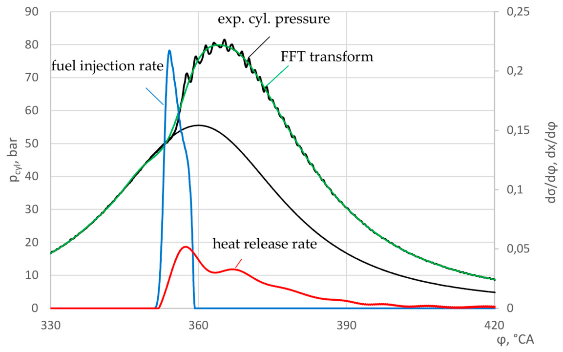
Each of the above-mentioned tasks requires the development of efficient computational algorithms and their implementation in software form. For example, accurate determination of the TDC position is performed using both the crankshaft position sensor signal and analysis of the compression curve of the experimental indicator diagram using methods proposed in [28,29,30]. Compensation for errors associated with crankshaft rotational speed irregularity is achieved using both direct signal acquisition from the flywheel toothed ring and analytical methods based on calculation of the resultant tangential force. FFT-based filtering algorithms are applied for determination of fuel ignition timing and calculation of heat release characteristics.
Figure 3.
Averaged and normalized experimental data for the test engine at (Pb = 18 kW at 1500 rpm) as a result of 72 consecutive cycles being processed.
Figure 3.
Averaged and normalized experimental data for the test engine at (Pb = 18 kW at 1500 rpm) as a result of 72 consecutive cycles being processed.
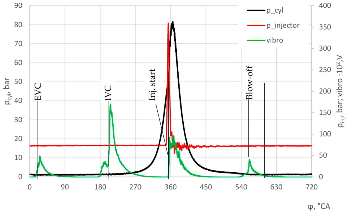
Figure 4.
Experimental cylinder pressure diagram superimposed with the calculated fuel injection rate diagrams and heat release rate diagrams for a test engine at mode (Pb = 18 kW at 1500 rpm).
Figure 4.
Experimental cylinder pressure diagram superimposed with the calculated fuel injection rate diagrams and heat release rate diagrams for a test engine at mode (Pb = 18 kW at 1500 rpm).
The following criteria were used for calibration of the mathematical model. For integral parameters averaged over the engine cycle, such as boost pressure, fuel consumption rate, and similar quantities, the objective function δint is proposed:
where N is the number of experimental operating points, is the experimentally measured value, and is the corresponding simulated value.
For the in-cylinder pressure diagram (indicator diagram), it is reasonable to use the parameter Δpav, defined as the average deviation between the simulated and experimental pressure traces over the engine cycle:
where L is the number of measurement points in the experimental indicator diagram.
The results of mathematical model calibration for three reference engine operating modes are presented in Figure 5 and Table 3.
Operating mode identification
From the perspective of mathematical modeling, the problem of identifying the current engine operating mode using sensor data requires accurate synthesis of fuel injection characteristics, fuel combustion characteristics, and proper determination of turbocharger turbomachinery parameters.
An important requirement is the automatic adjustment of the corresponding model calibration parameters based on the calibration data obtained at the reference operating points. As an example of such model adaptation, consider the fuel injection characteristics. Figure 6 presents the experimentally and computationally determined injection rate profiles for three reference operating modes of the investigated diesel-generator set: ,, and .
The obtained injection characteristics may be directly utilized within the digital twin; however, they remain valid only for the operating conditions under which they were determined. Therefore, the digital twin must be capable of modifying the fuel injection characteristics according to changes in the engine operating mode. In the case of a diesel-generator set, the parameter that primarily characterizes operating mode variations from the perspective of fuel injection is the injection duration, which can be experimentally determined through analysis of a vibroacoustic sensor signal.
In his work, Razleitsev [31] proposed approximating fuel injection characteristics using the sum of two parabola-type functions:
where is the normalized injection angle, Фinj1 is the relative duration of application of the first approximation function, and a, b, c, m1, m2, m3 and m4 are calibration coefficients.
Figure 6 shows the experimentally and computationally derived injection characteristics plotted as a function of the normalized injection angle . A common feature of all obtained curves can be observed during the initial injection phase, namely a gradual increase in the injection rate that closely follows an exponential trend.
Such behavior cannot be adequately represented by the original Razleitsev equations. However, satisfactory approximation can be achieved through a minor modification of the model:
where Фinj2 denotes the relative start point of application of the second approximation function.
When Фinj2 = 0, the original Razleitsev formulation is recovered. Appropriate selection of Фinj1 and Фinj2 enables satisfactory approximation of the initial stage of fuel injection.
Obviously, when the injection duration changes, the calibration parameters a, b, c, m1, m2, m3, m4, Фinj1 and Фinj2 must also change. However, for practical implementation within a digital twin, it is desirable to minimize the number of variable parameters. In the present case, satisfactory representation of the injection characteristics over the investigated operating range can be achieved by varying only three parameters: m4, Фinj1 and Фinj2.
Figure 7 presents the regression relationships obtained for these parameters as functions of the injection duration φinj. Application of the proposed fuel injection model to both the reference operating modes and an arbitrary intermediate operating mode is illustrated in Figure 8. The results demonstrate that the modified equations provide sufficiently accurate approximation of the experimental injection characteristics, including the critical initial stage of fuel injection.
Malfunction detection
To employ a digital twin for engine condition diagnostics, an optimization problem must be solved. One potentially effective approach is the application of Design of Experiments (DoE) methodology and statistical response surface analysis.
In particular, the following approach may be proposed. The engine is considered as a collection of interconnected systems and mechanisms, including the fuel injection system, air supply system, valve timing mechanism, cylinder–piston assembly, and others. For each system or mechanism, a set of parameters can be identified that reflects specific fault conditions and can be incorporated into the engine process simulation.
For the fuel injection system, such parameters may include the fuel injection timing, injection duration, injector nozzle hole diameter, and fuel density and viscosity. For the valve timing mechanism, the relevant parameters include intake and exhaust valve opening and closing timings. For the air supply system, characteristic parameters include charge-air cooler resistance and effectiveness, compressor and turbine adiabatic efficiencies, turbine flow capacity, exhaust system resistance, and similar quantities. The selection of parameters depends on the specific engine under investigation.
The fault identification procedure may be formulated as a sequential analysis of each selected engine subsystem. For this purpose, a numerical experiment is performed using either a full-factorial experimental design matrix or an appropriate fractional-factorial replica. For each parameter representing a potential fault, a baseline level and variation interval are specified. The objective functions are selected to quantify deviations between simulation results and diagnostic or monitoring data obtained from the actual engine.
For integral engine performance parameters, the objective function δint defined by Equation (14) is employed. For indicator diagrams, which remain one of the most informative diagnostic tools in marine engine practice, the following objective function is proposed:
where Δpav and Δpmax denote the average cycle deviation (defined according to Equation (15)) and the maximum deviation between experimental and simulated indicator diagrams, respectively.
For a more detailed analysis of indicator diagram discrepancies, logarithmic objective functions may also be introduced:
The logarithmic representation normalizes deviations across different phases of the engine cycle, particularly during combustion and gas-exchange processes. This feature is important when diagnosing faults originating from different engine subsystems.
Figure 9 illustrates simulation results obtained for a prototype engine, selected as the MAN B&W 8S50ME-B8 operating at 75% MCR along the propeller characteristic. A combined fault condition involving cylinder wear and exhaust valve malfunction was artificially introduced. It can be observed that the ln(p)=f(φ) diagram provides substantially better visualization of deviations during both combustion and gas-exchange phases than the conventional p=f(φ) indicator diagram.
The proposed fault identification methodology was evaluated using a test case. A digital twin was developed within the Blitz-PRO simulation environment based on a virtual engine derived from the MAN B&W 6S80ME-C7 prototype. A fault associated with the fuel injection system was simulated for one of the six cylinders while operating at 75% MCR along the propeller characteristic.
The input dataset available for fault detection consisted of measurements obtainable using standard engine instrumentation, as summarized in Table 4, together with the indicator diagram of the affected cylinder. Furthermore, it was assumed that the faulty subsystem was known in advance and that only two fault-related parameters deviated simultaneously from their healthy values.
All simulations were performed using a constant cycle fuel delivery of qf = 135.4 g/cycle. The following diagnostic factors were investigated:
- Injection timing φstart.inj, characterizing fuel pump adjustment quality and high-pressure fuel pump valve condition;
- Injection duration φinj, characterizing wear of fuel equipment and injector adjustment;
- Injector nozzle hole diameter dinj.holes, characterizing nozzle wear;
- Coefficient Ec in the fuel spray mean diameter correlation, characterizing deterioration of the injector needle valve.
Table 5 summarizes the baseline factor levels, variation intervals, and parameter values corresponding to both healthy (etalon) and faulty (malfunction) operating conditions.
Table 6 presents the fractional-factorial design matrix together with the corresponding values of the three objective functions δint, ΔpID, and Δln(p)ID. The same table also contains the calculated response surfaces obtained using second-order polynomial regression models. Figure 10 presents the synthesized indicator diagrams corresponding to different factor combinations.
The response functions were approximated using second-order polynomial regression equations of the form:
g(x1, x2, x3, x4) = a0 + a1⋅x1 + a2⋅x2 + a3⋅x3 + a4⋅x4 + a5⋅x1⋅x2 + a6⋅x1⋅x3 + a7⋅x1⋅x4 + a8⋅x2⋅x3 + a9⋅x2⋅x4+ a10⋅x3⋅x4 + a11⋅x12 + a12⋅x22 + a13⋅x32 + a14⋅x42
The coefficients ai for the three objective functions are provided in Table 7.
The obtained regression models were subsequently analyzed to locate their extrema and determine the factor combinations corresponding to the minimum objective function values. The results are presented in Table 8.
As can be seen, the analysis successfully identified the nature of the simulated malfunction, namely prolonged fuel injection (a possible consequence of leakage within the high-pressure fuel pump) combined with deteriorated fuel atomization (a possible consequence of injector nozzle wear). However, the exact numerical values of the fault-related parameters were not estimated accurately.
Consequently, the results demonstrate the importance of selecting factors with sufficiently independent physical effects when constructing the diagnostic experiment.
It is also informative to compare the optimized parameter values with the actual values used to simulate the malfunction. Such a comparison is presented in Figure 11. The results indicate that the parameter combinations identified through optimization reproduce the actual engine process with satisfactory accuracy, particularly for parameter set (3) shown in Figure 11.
4. Discussion
The presented results on engine condition diagnostics based on digital twin simulation demonstrate both the significant potential of the proposed approach and a number of challenges that must be addressed before its practical implementation in marine engine operation.
Indeed, provided that a properly calibrated digital twin is available, Design of Experiments (DoE) methods can be employed to investigate the influence of various faults and malfunctions within engine systems on the parameters of the working process. Furthermore, the proposed methodology enables estimation of the quantitative values of fault-related parameters, which can subsequently be verified during engine inspection and maintenance procedures.
An important advantage of the proposed approach is its potential for automation. In principle, the digital twin may continuously compare actual engine performance against the reference performance of a healthy engine and automatically identify probable causes of detected deviations. Such functionality could significantly enhance the capabilities of modern condition monitoring systems.
However, the conducted investigations have also revealed several challenges that require further research:
- Improvement of numerical experiment design and response surface analysis methods to ensure reliable identification of response function extrema and elimination of physically unrealistic solutions.
- The digital twin must incorporate physical parameters of engine systems and components that can be directly measured during condition assessment. This requirement necessitates an adequate level of model detail and adaptation of the mathematical model to the specific engine under consideration.
- The factors selected to represent potential faults should, as far as possible, influence the engine process independently and exhibit minimal correlation with one another.
Therefore, further development of the proposed methodology requires an appropriate level of physical detail within the engine model to represent the most probable fault mechanisms of a specific engine. This will facilitate the selection of diagnostic factors that satisfy the fundamental requirements of Design of Experiments theory, namely controllability, measurability, independence, compatibility, uniqueness, significance, and reproducibility.
In addition, practical implementation of the proposed approach under real operating conditions must account for cycle-to-cycle variability of the engine working process and uncertainties associated with measurement systems and sensors.
Following the successful validation of the methodology using a virtual test case, the next logical step is experimental verification on a research engine. Under real operating conditions, diagnostic procedures become substantially more challenging due to cycle-to-cycle combustion variability and measurement uncertainties affecting both conventional engine parameters and indicator diagrams.
To enable such investigations, controlled modifications of the engine working process must be introduced experimentally. For example, a throttle valve was installed upstream of the compressor inlet to simulate variations in intake system resistance, as illustrated in Figure 12. And Figure 13 presents an example of the resulting influence on engine performance. Additional factors that may be varied experimentally include fuel delivery parameters, exhaust system resistance, and fuel properties.
5. Conclusions
The application of digital twin technology to monitoring and diagnostic systems for marine internal combustion engines represents an important step toward more automated and efficient operation of marine power plants. Early detection of engine faults contributes not only to improved navigational safety and reduced risk of failures, but also to lower fuel and lubricant consumption and reduced environmental impact.
An engine digital twin should provide an adequate level of detail in the simulation of engine working processes and include, among its input variables, physical parameters describing the principal engine systems and components that may be associated with fault development. Particular importance is attached to the calibration of the mathematical model and to the integration of the digital twin with the actual engine through sensor-based data acquisition.
The digital twin enables both the establishment of reference engine performance based on manufacturer specifications and sea-trial data, and the continuous assessment of deviations between actual and reference operating parameters during service.
From a practical perspective, one of the most important advantages of the proposed approach is the ability to identify probable faults responsible for observed deviations from reference performance. To achieve this objective, the use of Design of Experiments methodology and numerical multifactor experiments has been proposed. By minimizing response functions associated with the selected objective functions, it becomes possible to estimate the values of fault-related parameters that characterize the engine condition.
The conducted investigations have demonstrated that successful fault identification strongly depends on the proper selection of factors and on accurate representation of their physical influence within the engine mathematical model. Particular attention should be paid to ensuring factor independence and compliance with the fundamental assumptions of experimental design theory.
Further development and practical implementation of the proposed methodology require consideration of cycle-to-cycle variability of engine working processes as well as measurement uncertainties associated with the sensors supplying input data to the digital twin.
Author Contributions
Conceptualization, D.M.; methodology, D.M.; software, D.M.; validation, D.M. and P.B.; formal analysis, R.V.; investigation, P.B.; resources, P.B.; data curation, Y.K.; writing—original draft preparation, D.M. and P.B.; writing—review and editing, R.V. and Y.K.; visualization, D.M.; supervision, D.M.; project administration, R.V.; funding acquisition, R.V. All authors have read and agreed to the published version of the manuscript.
Funding
This research received no external funding.
Data Availability Statement
The original contributions presented in this study are included in the article. Further inquiries can be directed to the corresponding authors. Additional information could be accessed by links: http://blitzpro.zeddmalam.com/application/index, https://depas.od.ua/.
Conflicts of Interest
the authors declare no conflicts of interest.
Abbreviations
The following abbreviations are used in this manuscript:
| DT | Digital twin |
| ICE | Internal combustion engine |
| TDC | Top dead center |
| BDC | Bottom dead center |
| EVO | Exhaust valve opening |
| EVC | Exhaust valve closing |
| IVO | Intake valve opening |
| IVC | Intake valve closing |
| ncrank | Engine speed |
| Pb | Brake power |
| p0 | Ambient pressure |
| pi | Indicator mean effective pressure |
| pmax | Maximum combustion pressure |
| pcompr | Compression pressure |
| pign | Pressure at the ignition point |
| ps | Charge air pressure |
| bb | Brake specific fuel consumption |
| boil | Specific fuel oil consumption |
| qfuel | Injected fuel mass per cycle |
| gNOx | Specific NOx emission |
| t0 | Ambient temperature |
| tt | Temperature at turbine inlet |
| tw1 | Cooling water temperature at engine inlet |
| toil1 | Oil temperature at engine inlet |
| poil1 | Oil pressure at engine inlet |
| φ | Crank angle (°CA) |
References
- Sagin, S.; Sagin, A.; Zablotskyi, Y.; Fomin, O.; Píštěk, V.; Kučera, P. Method for Maintaining Technical Condition of Marine Diesel Engine Bearings. Lubricants 2025, 13, 146. [Google Scholar] [CrossRef]
- Melnyk, O.M.; Shumylo, O.M.; Bulgakov, M.P.; Voronenko, S.V.; Onishchenko, O.A.; Korobkova, O.M.; Shapovalova, I.O.; Panteleieva, O.S. Integrated Multicriteria Analysis of Hydrogen and Ammonia as Alternative Marine Fuels in the Maritime Transport Decarbonization Process. J. Chem. Technol. 2025, 33, 1216–1231. [Google Scholar] [CrossRef]
- Shahmoradi, S.; Hosseini Imani, M.; Mazza, A.; Pons, E. Applications of the Digital Twin and the Related Technologies Within the Power Generation Sector: A Systematic Literature Review. Energies 2025, 18, 5627. [Google Scholar] [CrossRef]
- Booyse, W.; Wilke, D.N.; Heyns, P.S. Deep Digital Twins for Detection, Diagnostics and Prognostics. Mech. Syst. Signal Process. 2020, 140, 106612. [Google Scholar] [CrossRef]
- Everllence. Digital Marine Products—Sea Ahead: Join Our Digital Journey. Available online: https://www.everllence.com/marine/solutions/digital-marine-products (accessed on 10 May 2026).
- Wärtsilä. Operim—Operational Performance Improvement & Monitoring. Available online: https://www.wartsila.com/marine/services/gas-solutions-services/operim (accessed on 10 May 2026).
- WinGD. WinGD Integrated Digital Expert: Unlocking the Full Power; WinGD Brochure, 2022. Available online: https://wingd.com/media/qo3ikkz1/wingd-wide-brochure.pdf (accessed on 10 May 2026).
- WinGD. WiDE (WinGD Integrated Digital Expert). Available online: https://wingd.com/products-solutions/digital-optimisation/wide (accessed on 10 May 2026).
- Wang, K.; Wang, X.; Tan, C.; Dong, S.; Zhao, F.; Lian, S. Digital twin-enhanced robotic system for remote diesel engine assembly defect inspection. Ind. Robot 2025, 52, 266–276. [Google Scholar] [CrossRef]
- Söderäng, E.; Hautala, S.; Mikulski, M.; Storm, X.; Niemi, S. Development of a digital twin for real-time simulation of a combustion engine-based power plant with battery storage and grid coupling. Energy Convers. Manag. 2022, 266, 115793. [Google Scholar] [CrossRef]
- Dong, X.; Huang, J.; Luo, N.; Hu, W.; Lei, Z. Design and Implementation of Digital Twin Diesel Generator Systems. Energies 2023, 16, 6422. [Google Scholar] [CrossRef]
- Koeser, P.S.; Berbig, F.; Pohlmann-Tasche, F.; Dinkelacker, F.; Wang, Y.; Tian, T. Predictive Piston Cylinder Unit Simulation - Part II: Novel Methodology of Friction Simulation Validation Utilizing Floating-Liner Measurements. In Proceedings of the SAE 2023 World Congress Experience (WCX 2023), Detroit, MI, USA, 18–20 April 2023; p. Paper No. 2023-01-0415. [Google Scholar] [CrossRef]
- Stoumpos, S.; Theotokatos, G.; Mavrelos, C.; Boulougouris, E. Towards Marine Dual Fuel Engines Digital Twins—Integrated Modelling of Thermodynamic Processes and Control System Functions. J. Mar. Sci. Eng. 2020, 8, 200. [Google Scholar] [CrossRef]
- Stoumpos, S.; Theotokatos, G. A novel methodology for marine dual fuel engines sensors diagnostics and health management. Int. J. Engine Res. 2022, 23, 974–994. [Google Scholar] [CrossRef]
- Geertsma, R.D.; Negenborn, R.R.; Visser, K.; Hopman, J.J. Design and control of hybrid power and propulsion systems for smart ships: A review of developments. Appl. Energy 2017, 194, 30–54. [Google Scholar] [CrossRef]
- Dong, X.; Huang, J.; Luo, N.; Hu, W.; Lei, Z. Design and Implementation of Digital Twin Diesel Generator Systems. Energies 2023, 16, 6422. [Google Scholar] [CrossRef]
- Aliramezani, M.; Koch, C.R.; Shahbakhti, M. Modeling, diagnostics, optimization, and control of internal combustion engines via modern machine learning techniques: A review and future directions. Prog. Energy Combust. Sci. 2022, 88, 100967. [Google Scholar] [CrossRef]
- Huang, Q.; Xie, T.; Liu, J. Machine Learning-Assisted Reconstruction of In-Cylinder Pressure in Internal Combustion Engines Under Unmeasured Operating Conditions. Energies 2025, 18, 5235. [Google Scholar] [CrossRef]
- Huang, Q.; Xie, T.; Liu, J. Machine Learning-Assisted Reconstruction of In-Cylinder Pressure in Internal Combustion Engines Under Unmeasured Operating Conditions. Energies 2025, 18, 5235. [Google Scholar] [CrossRef]
- Hanuschkin, A.; Schober, S.; Bode, J.; Schorr, J.; Böhm, B.; Krüger, C.; Peters, S. Machine learning–based analysis of in-cylinder flow fields to predict combustion engine performance. Int. J. Engine Res. 2021, 22, 257–272. [Google Scholar] [CrossRef]
- Nath, K.; Kumar, V.; Smith, D.J.; Karniadakis, G.E. A digital twin for diesel engines: Operator-infused physics-informed neural networks with transfer learning for engine health monitoring. Eng. Appl. Artif. Intell. 2026, 170, 114052. [Google Scholar] [CrossRef]
- Deon, B.; Cotta, K.P.; Silva, R.F.V.; Batista, C.B.; Justino, G.T.; Freitas, G.C.; Cordeiro, A.M.; Barbosa, A.S.; Loução, F.L.; Simioni, T.; et al. Digital twin and machine learning for decision support in thermal power plant with combustion engines. Knowl.-Based Syst. 2022, 253*, 109578. [Google Scholar] [CrossRef]
- Bo, Y.; Wu, H.; Che, W.; Zhang, Z.; Li, X.; Myagkov, L. Methodology and application of digital twin-driven diesel engine fault diagnosis and virtual fault model acquisition. Eng. Appl. Artif. Intell. 2024, 131, 107853. [Google Scholar] [CrossRef]
- Wu, W.-H.; Chen, G.-B.; Yang, Z.-C. The Application and challenge of Digital Twin technology in Ship equipment. Proceedings of the 2021 International Conference on Mechanical Engineering, Intelligent Manufacturing and Automation Technology (MEMAT 2021) J. Phys. Conf. Ser. 2021, 2021(1939), 012068. [Google Scholar] [CrossRef]
- Korczewski, Z.; Varbanets, R.; Minchev, D.; Rudnicki, J. Multi-Symptom Diagnostic Investigation of the Working Process of a Marine Diesel Engine: Case Study Part 2 Simulation Diagnostics. Pol. Marit. Res. 2025, 32(4), 87–96. [Google Scholar] [CrossRef]
- Minchev, D.S.; Varbanets, R.A.; Alexandrovskaya, N.I.; Pisintsaly, L.V. Marine diesel engines operating cycle simulation for diagnostics issues. Acta Polytech. 2021, 61, 435–447. [Google Scholar] [CrossRef]
- Varbanets, R.; Minchev, D.; Savelieva, I.; Rodionov, A.; Mazur, T.; Psariuk, S.; Bondarenko, V. Advanced marine diesel engines diagnostics for IMO decarbonization compliance. AIP Conf. Proc. 2024, 3104, 020004. [Google Scholar] [CrossRef]
- Minchev, D.; Varbanets, R.; Shumylo, O.; Zalozh, V.; Aleksandrovska, N.; Bratchenko, P.; Truong, T.H. Digital Twin Test-Bench Performance for Marine Diesel Engine Applications. Pol. Marit. Res. 2023, 30, 81–91. [Google Scholar] [CrossRef]
- Korczewski, Z.; Rudnicki, J.; Varbanets, R.; Minchev, D. Multi-Symptom Diagnostic Investigation of the Working Process of a Marine Diesel Engine: Case Study Part 1 Measurement Diagnostics. Pol. Marit. Res. 2025, 32(2), 50–61. [Google Scholar] [CrossRef]
- Varbanets, R.; Minchev, D.; Zalozh, V.; Marchenko, A.; Gryshchuk, Y.; Klymenko, V. Methods of Real-Time Parametric Diagnostics for Marine Diesel Engines. Pol. Marit. Res. 2024, 31, 71–84. [Google Scholar] [CrossRef]
- Razleytsev, N.F. Modelirovanie i Optimizatsiya Protsessa Sgoraniya v Dizelyakh [Modeling and Optimization of the Combustion Process in Diesel Engines]; Vishcha Shkola: Kharkiv, Ukraine, 1980; p. 169. [Google Scholar]
Figure 1.
Sets of operating modes, technical states and monitoring parameters and their interrelation.
Figure 1.
Sets of operating modes, technical states and monitoring parameters and their interrelation.
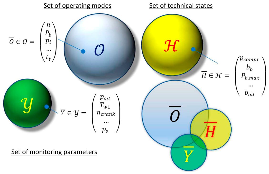
Figure 2.
Digital Twin framework for diagnostics task.
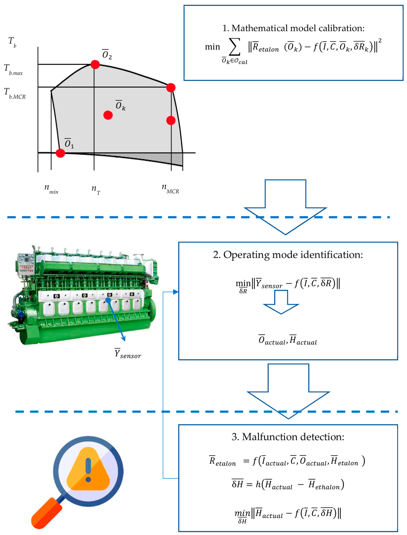
Figure 5.
Simulated and experimental indicated diagrams after mathematical model calibration.
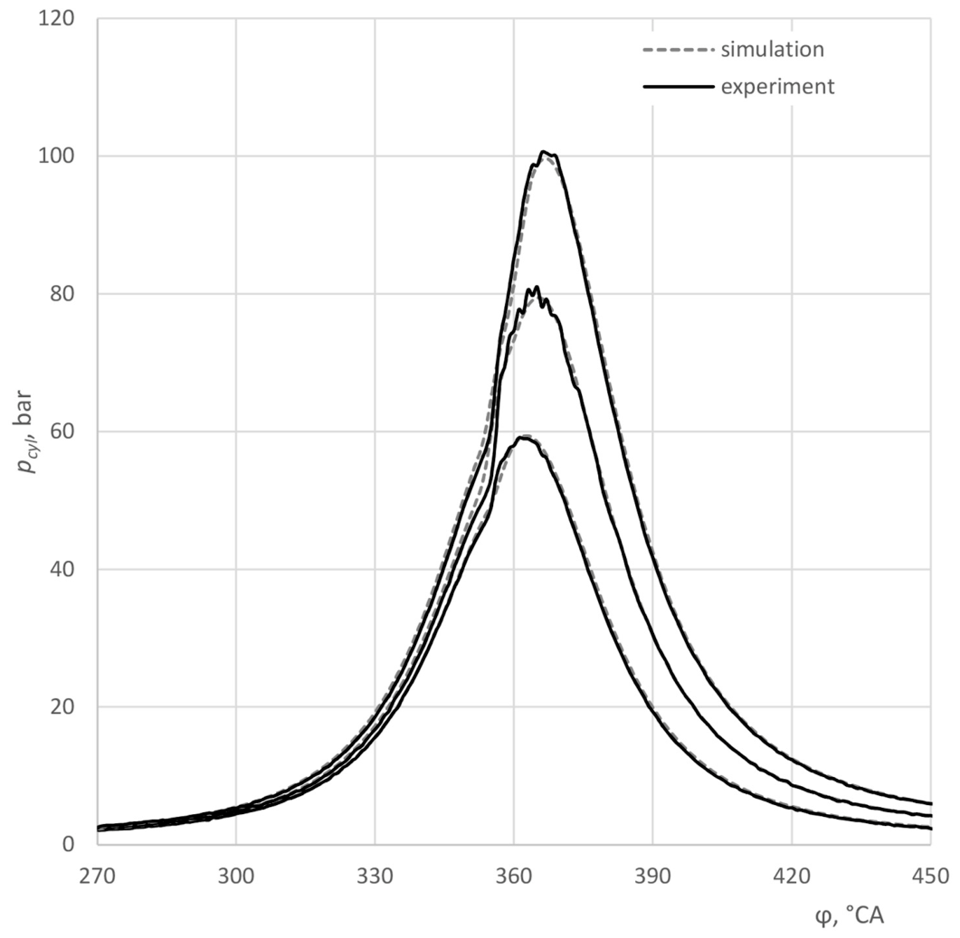
Figure 6.
Fuel-injection diagrams for three operating mode at 1500 rpm.
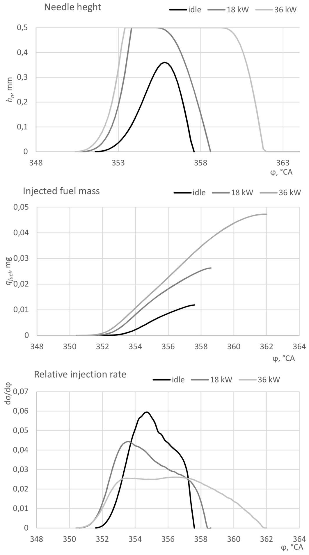
Figure 7.
Regressions for chosen coefficients of injection characteristics prediction.
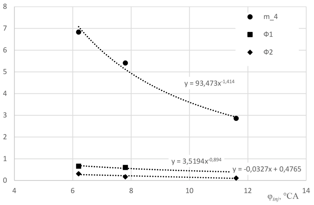
Figure 8.
Experimental and simulated fuel injection diagrams: a) 36 kW, b) 18 kW, c) idle, d) random (φinj = 10 °CA). .
Figure 8.
Experimental and simulated fuel injection diagrams: a) 36 kW, b) 18 kW, c) idle, d) random (φinj = 10 °CA). .
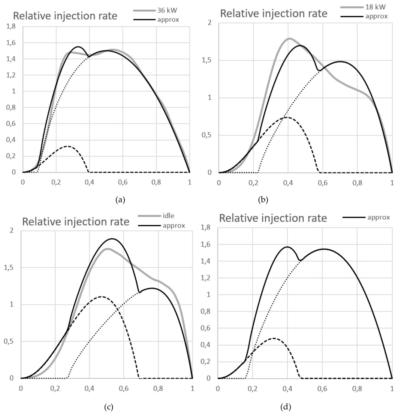
Figure 9.
Fractional experiment simulations diagrams for MAN B&W 8S50ME-B8 at valvetrain system and cylinder wear malfunction.
Figure 9.
Fractional experiment simulations diagrams for MAN B&W 8S50ME-B8 at valvetrain system and cylinder wear malfunction.
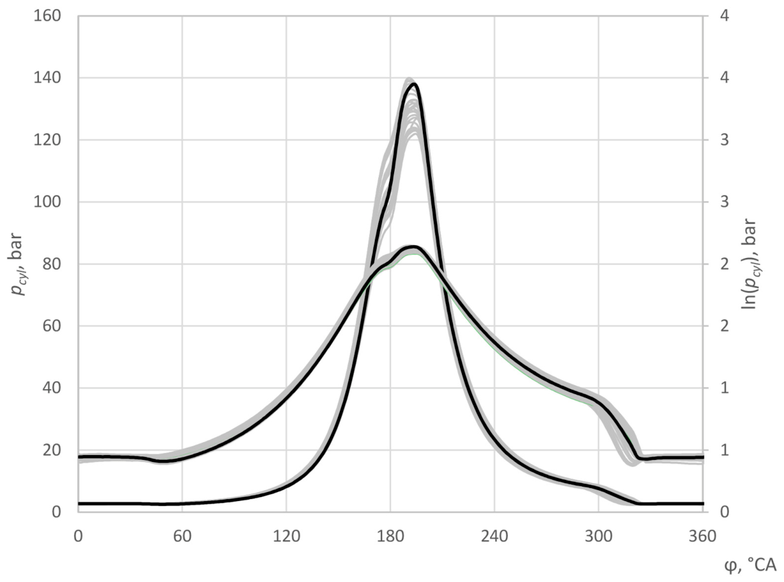
Figure 10.
Fractional experiment simulations diagrams for MAN B&W 6S80ME-С7 at fuel-injection system malfunction.
Figure 10.
Fractional experiment simulations diagrams for MAN B&W 6S80ME-С7 at fuel-injection system malfunction.
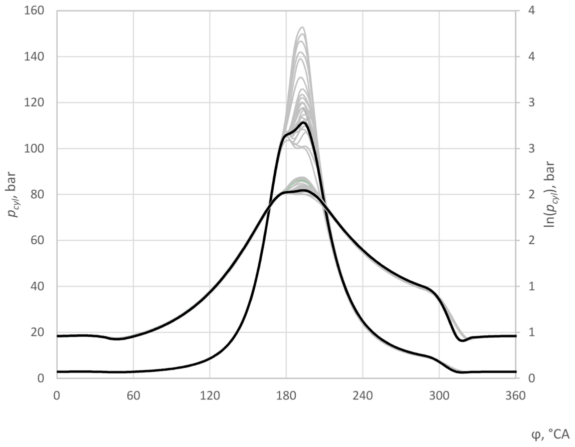
Figure 11.
Comparison of pressure traces for three sets of varying factors φstart.inj, φinj, dinj.holes, Ec (output from Blitz-PRO service): 1) 2, 24, 1.2, 1.15; 2) 0.2, 26, 1.4, 1.15; 3) 2, 26, 1.2, 1.25.
Figure 11.
Comparison of pressure traces for three sets of varying factors φstart.inj, φinj, dinj.holes, Ec (output from Blitz-PRO service): 1) 2, 24, 1.2, 1.15; 2) 0.2, 26, 1.4, 1.15; 3) 2, 26, 1.2, 1.25.
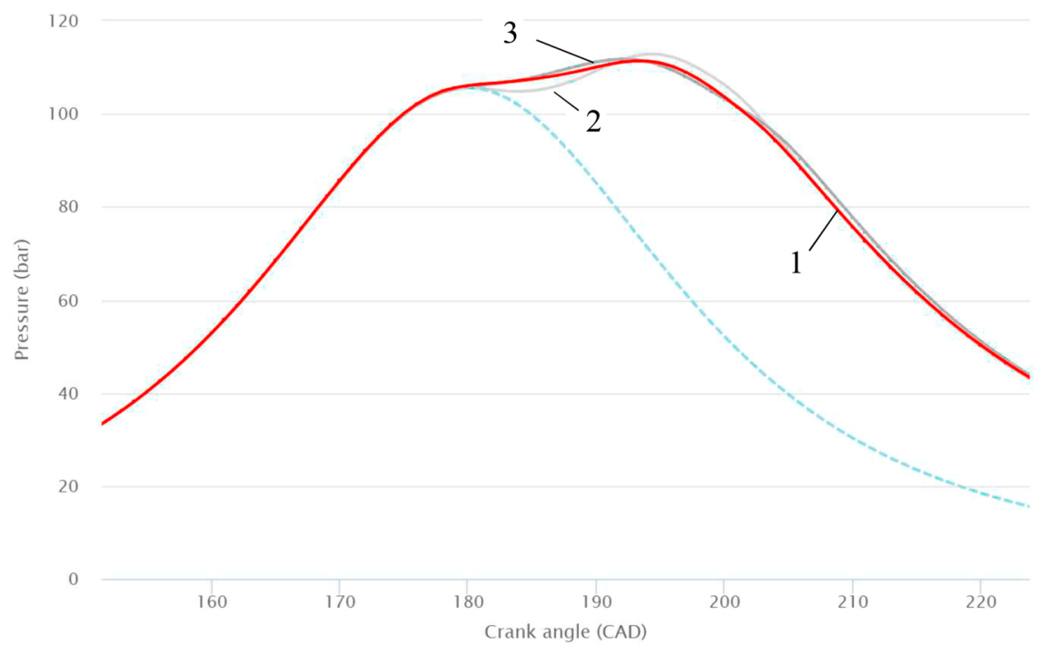
Figure 12.
Throttle valve installation on the test engine.
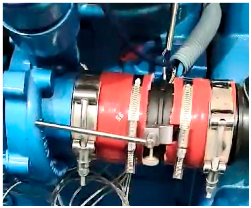
Figure 13.
Depas 5.0W diagnostic system report for 18 kW without throttling (left) and with throttling (right).
Figure 13.
Depas 5.0W diagnostic system report for 18 kW without throttling (left) and with throttling (right).
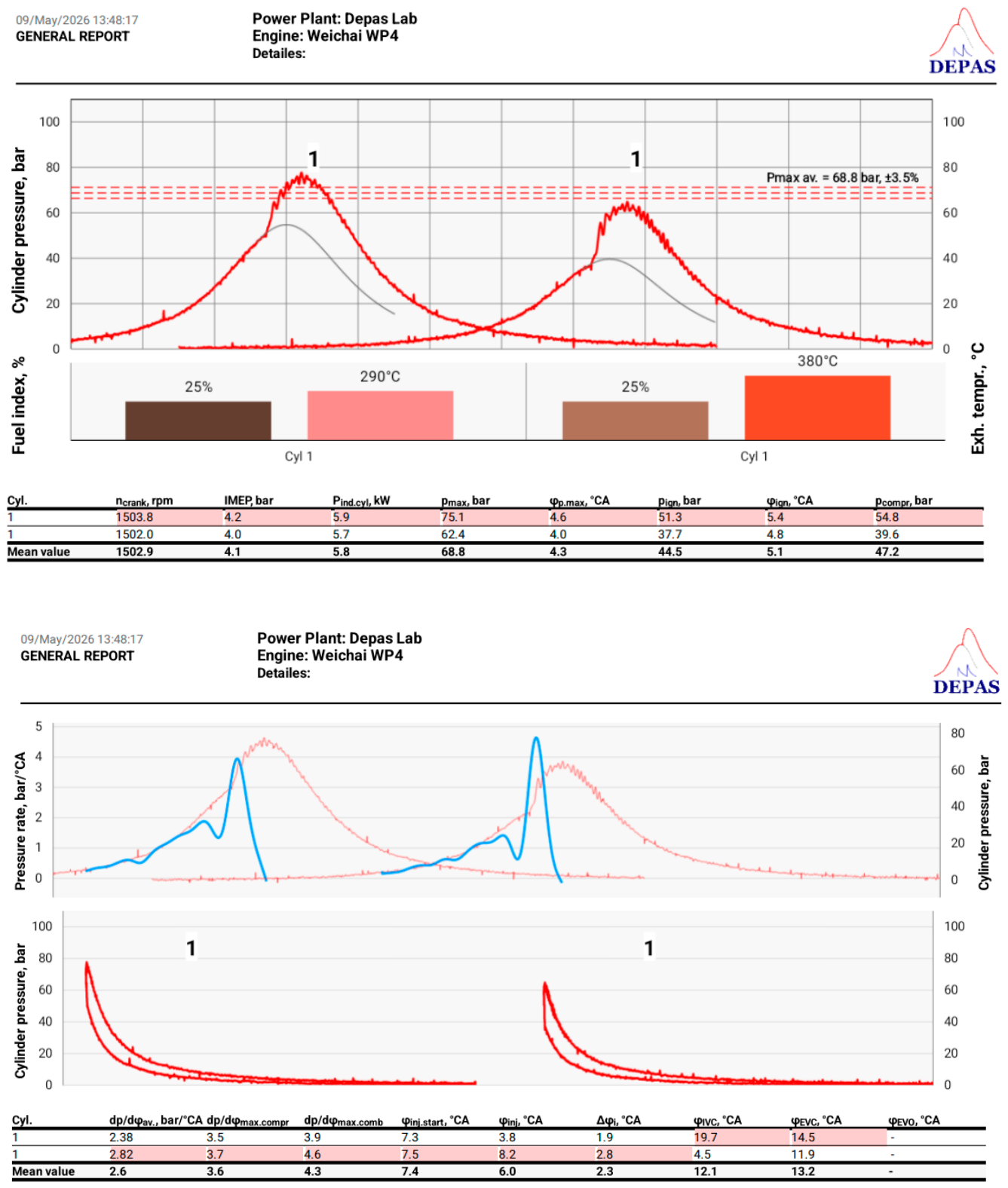

Table 1.
Set of operating modes used for mathematical model calibration.
| № | Designation | Pb, kW | ncrank, rpm |
| 1 | 0 | 670 | |
| 2 | 0 | 1500 | |
| 3 | 18 | 1500 | |
| 4 | 36 | 1500 |
Table 2.
Example of the vector for the operating mode .
| № | Parameter | Units | Value | Accuracy |
| Parameters of the operating mode | ||||
| 1 | Pb | kW | 18,5 | ± 0.1 |
| 2 | ncrank | rpm | 1509.3 | ± 0.1 |
| 3 | p0 | bar | 1.01 | ± 0.01 |
| 4 | t0 | °C | 10 | ± 0.1 |
| 5 | tw1 | °C | 80 | ± 0.5 |
| 6 | toil1 | °C | 75 | ± 0.5 |
| Experimental data | ||||
| 7 | pcyl = f(φ) | bar | Arrays of data, visualization as diagrams (see Figure 3 for example) | 1 % |
| 8 | pinj = f(φ) | bar | 1 % | |
| 9 | ppump = f(φ) | bar | 1 % | |
| 10 | flywheel = f(φ) | V | - | |
| 11 | Vvibro = f(φ) | V | - | |
| 12 | ps | bar | 1.15 | ± 0.01 |
| 13 | ts | °C | 43.3 | ± 0.1 |
| 14 | Gair | kg/s | ± 0.005 | |
| 15 | Gfuel | kg/h | 4.62 | ± 0.005 |
| 16 | tt / tt2 | °C | 281.5 / 258.3 | ± 0.5 |
| 17 | tt.cyl1, tt.cyl2, tt.cyl3, tt.cyl4 | °C | 267.3, 252.5, 279.3, 235.5 |
± 0.5 |
| 18 | [CO] | ppm | 80.4 | 2 % |
| 19 | [NOx] | ppm | 1230 | 2 % |
| 20 | [O2] | % | 15.4 | 2 % |
| Manufacturer data | ||||
| 21 | ε | - | 18 | - |
| 22 | bb | kg/(kW·h) | - | |
| 23 | φIVC | °CA after BDC | 20 | - |
| 24 | φIVO | °CA before TDC | 9 | - |
| 25 | φEVC | °CA after TDC | 18 | - |
| 26 | φ EV0 | °CA before BDC | 42 | - |
| Outcome of experimental data processing | ||||
| 27 | pi | bar | 3.97 | ± 0.01 |
| 28 | bi | kg/(kW·h) | 173.8 | ± 0.5 |
| 29 | pmax | bar | 79.4 | ± 0.5 |
| 30 | pc | bar | 57 | ± 0.5 |
| 31 | pign | bar | 52.8 | ± 0.5 |
| 32 | φIVC | °CA after BDC | 20.2 | ± 0.5 |
| 33 | φIVO | °CA before TDC | ||
| 34 | φEVC | °CA after TDC | 19.8 | ± 0.5 |
| 35 | φEV0 | °CA after TDC | ||
| 36 | φign | °CA before TDC | 5.7 | ± 0.5 |
| 37 | φinj.start | °CA before BDC | 9 | ± 0.5 |
| 38 | φinj | °CA | 8 | ± 0.5 |
| 39 | dσ/dφ = f(φ) | - | ||
| 40 | dx/dφ = f(φ) | - | ||
Table 3.
Mathematical model calibration accuracy.
| Operating mode | Engine power | δint , % | Δpav , bar |
| 0 | 1.26 | 0.059 | |
| 18 | 1.13 | 0.216 | |
| 36 | 1.52 | 0.235 |
Table 4.
Set of data from sensors for a 75% MCR propeller load operation of the virtual engine MAN B&W 6S80ME-C7.
Table 4.
Set of data from sensors for a 75% MCR propeller load operation of the virtual engine MAN B&W 6S80ME-C7.
| Parameter | Units | Etalon | Malfunction |
| Indicated mean effective pressure, IMEP | bar | 16.66 | 15.99 |
| Maximum pressure, pmax | bar | 120.3 | 111.3 |
| Compression pressure, pcomp | bar | 107.5 | 105.7 |
| Exhaust gas temperature after exhaust valve, texh | °C | 376.5 | 405 |
| Scavenge air receiver pressure, pres | bar | 2.94 | 2.93 |
| Scavenge air cooler air inlet temperature, tk | °C | 142 | 140.8 |
| Air pressure drop across scavenge air cooler, ΔpCAC | bar | 0.02 | 0.02 |
| Air pressure drop across air intake filter, Δpint | bar | 0.01 | 0.01 |
| Scavenge air receiver temperature, tres | °C | 46.4 | 46.5 |
| T/C air intake temperature, tint | °C | 20 | 20 |
Table 5.
Values of variable factors.
| Parameter | Units | Base level | Interval of variation | Etalon value | Malfunction value |
| φstart.inj | °CA | 2 | 3 | 2 | 2 |
| φinj | °CA | 23 | 3 | 20 | 24 |
| dinj.holes | mm | 1.3 | 0.1 | 1.2 | 1.35 |
| Ec | - | 1.2 | 0.05 | 1.15 | 1.15 |
Table 6.
Replica of the full-factor numerical experiment for the set of controlled parameters.
| № | Factors | Target functions | Regression | |||||||
| φstart.inj | φinj | dinj.holes | Ec | δint | ΔpID | Δln(p)ID | δ’int | Δp’ID | Δln(p)’ID | |
| °CA | °CA | mm | - | % | bar | - | % | bar | - | |
| 1 | 2 | 20 | 1.4 | 1.25 | 1.37 | 2.64 | 0.0114 | 1.58 | 3.14 | 0.0159 |
| 2 | 2 | 20 | 1.2 | 1.25 | 3.28 | 5.54 | 0.0223 | 2.91 | 4.91 | 0.0197 |
| 3 | 2 | 26 | 1.2 | 1.25 | 0.64 | 0.99 | 0.0059 | 1.01 | 1.32 | 0.0047 |
| 4 | 2 | 23 | 1.2 | 1.25 | 3.05 | 4.30 | 0.0190 | 2.44 | 3.26 | 0.0209 |
| 5 | 5 | 20 | 1.2 | 1.25 | 9.54 | 17.34 | 0.0671 | 9.61 | 17.50 | 0.0651 |
| 6 | -1 | 20 | 1.3 | 1.25 | 2.47 | 3.98 | 0.0537 | 2.80 | 4.65 | 0.0531 |
| 7 | 2 | 20 | 1.4 | 1.2 | 1.59 | 3.54 | 0.0141 | 1.90 | 3.64 | 0.0108 |
| 8 | 2 | 20 | 1.4 | 1.2 | 4.18 | 6.62 | 0.0265 | 3.45 | 5.66 | 0.0204 |
| 9 | 2 | 26 | 1.4 | 1.2 | 1.28 | 1.48 | 0.0080 | 1.46 | 2.31 | 0.0070 |
| 10 | 2 | 23 | 1.4 | 1.2 | 3.66 | 5.15 | 0.0222 | 3.04 | 4.26 | 0.0254 |
| 11 | 5 | 20 | 1.2 | 1.2 | 10.09 | 18.51 | 0.0704 | 10.77 | 19.48 | 0.0756 |
| 12 | -1 | 20 | 1.2 | 1.2 | 2.96 | 4.72 | 0.0538 | 3.15 | 4.67 | 0.0559 |
| 13 | 2 | 26 | 1.2 | 1.15 | 3.54 | 5.27 | 0.0238 | 2.34 | 3.61 | 0.0193 |
| 14 | 2 | 23 | 1.2 | 1.15 | 0.51 | 0.69 | 0.0044 | 1.69 | 2.45 | 0.0118 |
| 15 | 5 | 20 | 1.3 | 1.15 | 6.15 | 12.26 | 0.0455 | 6.01 | 11.95 | 0.0474 |
| 16 | -1 | 20 | 1.3 | 1.15 | 1.10 | 2.74 | 0.0115 | 0.73 | 2.37 | 0.0055 |
| 17 | 2 | 26 | 1.3 | 1.15 | 0.58 | 1.29 | 0.0055 | 1.72 | 2.78 | 0.0069 |
| 18 | 2 | 23 | 1.3 | 1.15 | 2.12 | 3.00 | 0.0129 | 2.26 | 3.17 | 0.0134 |
| 19 | 5 | 20 | 1.4 | 1.15 | 8.88 | 16.13 | 0.0640 | 8.56 | 16.03 | 0.0594 |
| 20 | -1 | 20 | 1.2 | 1.15 | 1.58 | 2.82 | 0.0133 | 1.71 | 2.85 | 0.0247 |
| 21 | 5 | 26 | 1.2 | 1.15 | 5.35 | 9.15 | 0.0357 | 5.11 | 8.89 | 0.0351 |
| 22 | -1 | 26 | 1.2 | 1.15 | 1.26 | 4.50 | 0.0193 | 1.00 | 3.79 | 0.0253 |
| 23 | 5 | 23 | 1.2 | 1.15 | 7.98 | 14.20 | 0.0600 | 7.93 | 13.75 | 0.0601 |
| 24 | -1 | 23 | 1.3 | 1.15 | 1.68 | 2.37 | 0.0544 | 1.66 | 2.82 | 0.0414 |
Table 7.
Coefficients of regression equations for selected target functions.
| a0 | a1 | a2 | a3 | a4 | a5 | a6 | a7 | |
| δint | -9.57E+01 | 9.07E+00 | -6.82E+00 | -1.16E+02 | 4.08E+02 | -1.20E-01 | -2.62E+00 | -2.68E+00 |
| ΔpID | -1.59E+02 | 2.20E+01 | -1.01E+01 | -1.66E+02 | 6.20E+02 | -3.24E-01 | -6.00E+00 | -6.55E+00 |
| Δln(p)ID | -1.14E+00 | 1.40E-02 | -4.26E-02 | -2.53E+00 | 5.25E+00 | -4.89E-04 | 1.21E-02 | -2.59E-02 |
| a8 | a9 | a10 | a11 | a12 | a13 | a14 | ||
| δint | 3.99E+00 | 1.04E+00 | 4.40E+01 | 2.40E-01 | 1.00E-02 | -9.90E+00 | -2.01E+02 | |
| ΔpID | 5.18E+00 | 9.32E-03 | 5.05E+01 | 4.92E-01 | 7.99E-02 | -2.20E+00 | -2.81E+02 | |
| Δln(p)ID | 4.66E-02 | 1.45E-02 | 1.18E+00 | 3.92E-03 | -7.32E-04 | 2.16E-02 | -2.87E+00 |
Table 8.
Estimation of factors values by regression functions extremums analysis.
| Parameter | Units | From functions extremums | Actual values | ||
| δ'int | Δp’ID | Δln(p)’ID | |||
| φstart.inj | °CA | 0.2 | 2 | 2 | 2 |
| φinj | °CA | 20 | 26 | 26 | 24 |
| dinj.holes | mm | 1.4 | 1.2 | 1.2 | 1.35 |
| Ec | - | 1.15 | 1.25 | 1.25 | 1.15 |
Disclaimer/Publisher’s Note: The statements, opinions and data contained in all publications are solely those of the individual author(s) and contributor(s) and not of MDPI and/or the editor(s). MDPI and/or the editor(s) disclaim responsibility for any injury to people or property resulting from any ideas, methods, instructions or products referred to in the content. |
© 2026 by the authors. Licensee MDPI, Basel, Switzerland. This article is an open access article distributed under the terms and conditions of the Creative Commons Attribution (CC BY) license.
Copyright: This open access article is published under a Creative Commons CC BY 4.0 license, which permit the free download, distribution, and reuse, provided that the author and preprint are cited in any reuse.


