

Submitted:
13 July 2026
Posted:
15 July 2026
You are already at the latest version
Abstract
This study validates the URANS k-ω SST turbulence model in OpenFOAM for simulating 2D flow around a fixed circular cylinder, a key benchmark for offshore structure design. Balancing accuracy and computational cost, the model was tested for laminar (Re=40) and subcritical turbulent (Re=10,000) regimes. Results showed excellent agreement with benchmarks: for laminar flow, a drag coefficient (Cd) of 1.54 and separation angle of 52.3°; for turbulent flow, a mean Cd of 1.15, a Strouhal number of 0.22 at x/D=2, and a separation angle of 86.5°. This confirms the model's reliability for predicting integral forces and vortex shedding in these regimes. However, the study also highlights the inherent limitations of the 2D domain due to its inability to resolve 3D anisotropic wake turbulence.
Keywords:
CFD
; OpenFOAM
; cylinder
; URANS
; k-ω SST
; vortex-induced vibration
1. Introduction
The investigation into the fluid flow dynamics around a fixed circular cylinder, a system renowned for its deceptive geometric simplicity and underlying flow complexity, remains one of the classical benchmarks in Computational Fluid Dynamics (CFD) for problems relevant to civil, naval, and coastal engineering [1,2,3,4]. An accurate predictive capacity is paramount for the robust design and safety assessment of modern offshore infrastructure, such as risers, monopile foundations, and bridge piers, where extreme turbulent flow and associated forces are prevalent [5,6,7]. Engineering applications typically encounter flow fields characterized by high Reynolds numbers (Re), which span a transitional range from the subcritical (Re~106) to the supercritical (Re~107) flow regimes [8,9]. Within this highly dynamic Re spectrum, the flow exhibits sequential transitions that lead to turbulent boundary layer separation and pronounced alternating pressure gradients, which in turn drive unsteady structural loading, the mechanism behind Vortex-Induced Vibration (VIV) [4,5,10]. The study of flow around a circular cylinder has evolved from early experimental classifications to advanced numerical simulations, focusing on boundary layers, shear layers, and wake dynamics.
High-fidelity models, including Direct Numerical Simulation (DNS) and highly resolved LES, provide the most detailed turbulent flow solution [9], yet they are rendered impractical for most industrial-scale applications by the astronomical computational resources required for modeling high Re, 3D, and lengthy transient simulations [3,10,11]. Therefore, the Unsteady Reynolds-Averaged Navier-Stokes (URANS) approach remains the necessary, reliable tool for large-scale engineering problems [12]. This research leverages the OpenFOAM platform, which, as an open-source CFD toolbox based on the Finite Volume Method (FVM), affords both computational efficiency (through message passing interface (MPI) parallelization) and the full flexibility required for customizing solvers (pisoFoam, pimpleFoam) and implementing advanced fluid model extensions crucial for simulating WSI (Wave-Structure Interaction) with tools like waves2Foam and olaFlow [13,14,15]. Given its superior performance over k-ε models in complex separated flow where turbulent viscosity modeling is crucial, the Shear Stress Transport (k-ω SST) model serves as the most suitable primary closure for URANS in external flow simulations [3,16].
The flow past a cylinder is partitioned into different fluid dynamic regimes across the full spectrum of Reynolds number. A fundamental contribution was provided by [1], who established a comprehensive phenomenological classification system based on three transitions in disturbed regions: the wake, the shear layers, and the boundary layers. Historically, early experimentalists such as [7,17,18] mapped these regimes.
The formation of vortices is the dominant feature of the wake, and its structure is highly sensitive to Reynolds number and three-dimensional (3D) instabilities. Norberg [19] provided an extensive review of fluctuating lift and wake modes, highlighting that in the subcritical regime, intrinsic 3D instabilities arise, specifically streamwise vortex loops (Mode A) and fine-scale streamwise rib structures (Mode B). Khan et al. (2018) [20] emphasized that the flow is inherently 3D at this Re=3900; 2D simulations fail to capture the turbulence decay mechanism, leading to overpredicted drag and historical discrepancies in recirculation length and separation angle. Rodríguez et al. (2015) [21] utilized Large Eddy Simulation (LES) to investigate the topology during the critical to supercritical transition (Re = 2.5105 to 8.5105). They confirmed the existence of asymmetric flow states characterized by one-bubble (asymmetrical) and two-bubble (symmetrical and asymmetrical) separation modes. As the flow progresses into the supercritical regime, the wake recovers symmetry, stabilizing into a narrower wake (thus, from approximately 0.87D in the critical regime to 0.4D in the supercritical regime) with a steady Strouhal number (St0.44), significantly higher than the subcritical value of 0.2 [21].
The forces exerted on the cylinder are decomposed into mean drag, fluctuating drag, and fluctuating lift; these forces can induce Vortex Induced Vibration (VIV). As detailed by [8,11], the mean drag coefficient drops suddenly during the critical regime due to the delay in separation points. Capturing this “drag crisis” is a primary benchmark for numerical models. Norberg [19] noted that while mean lift is zero for a symmetric cylinder, the fluctuating lift (RMS) is significant due to alternating vortex shedding. The spanwise correlation length of these forces is highly dependent on Re, dropping significantly during the transition regimes. Vlastos [10] and He [8] describe the “lock-in” phenomenon, where the vortex shedding frequency synchronizes with the structure’s natural frequency, leading to high-amplitude vibrations. He [8] further explored VIV in tapered cylinders and shear flows, establishing that structural shear rates (varying diameter) can broaden the lock-in bandwidth compared to uniform cylinders.
With the advent of CFD, the URANS became the suitable choice for industrial applications. Pang [3] and Ong [11] evaluated various turbulence models, their results indicated that the Standard k-ε model is robust but often over-predicts turbulence in the stagnation region. Menter’s k-ω SST (Shear Stress Transport) model is widely regarded as superior for cylinder flows. Rosetti [9] URANS calculations for smooth circular cylinder flow in a wide range of Reynolds numbers: solution verification and validation URANS calculations for smooth circular cylinder flow in a wide range of Reynolds numbers: solution verification and validation performed a rigorous verification and validation study, concluding that URANS captures global quantities (mean drag, Strouhal number) reasonably well for Re = 10 to 5105, including the general trends of the drag crisis. However, [2,9] highlight that URANS assumes isotropic eddy viscosity, which fails to reproduce the 3D streamwise vorticity in the subcritical wake. This often leads to an overestimation of drag and base suction (shorter formation lengths) compared to experimental data, particularly in the critical regime where boundary layer transition is highly sensitive.
To capture the stochastic nature of turbulence and 3D wake structures, researchers moved resorted to the LES model. Catalano [8] and Rodríguez [21] demonstrated that LES provides superior accuracy in the critical and supercritical regimes, correctly capturing the delayed separation and the recovery of the drag coefficient. Khan [20] demonstrated that spanwise mesh resolution is critical; coarse grids act like 2D simulations, artificially enhancing coherence and overpredicting forces. They recommended specific grid densities for wall-resolved LES. Catalano et al. (2003) [8] noted that wall-resolved LES becomes less suitable at Re > 106, necessitating wall-functions or hybrid RANS-LES (DES) approaches.
The numerical validation of URANS models (the primary focus in studies up to (Re ~ 106) illustrates a hierarchy of model performance when constrained by buoyancy or separation effects [3,10]. Firstly, simpler linear EVMs (such as k-ε) generally yield unsatisfactory results for flow past a cylinder due to model breakdown at separated regions (i.e., overestimating separation angle ), consequently failing to correctly predict lift and drag dynamics, and exhibiting inappropriate eddy-viscosity fields when turbulence is generated anisotropically [3,10,12,13]. This flawed prediction of the separation point remains the critical reason for predictive inaccuracy. Secondly, the k-ω SST model has been rigorously selected for high-Re flows for its superior stability in separated regions and for the flexibility of enhancement [16,17]. Comparative OpenFOAM work by [3] demonstrated the importance of augmenting this closure via features like curvature correction, which improved the accuracy of Cd and St by mitigating the turbulence models’ poor performance in high-shear, rotational regions. Thirdly, Scale-Resolving and Hybrid models (DES, LES, WALE LES) offer necessary compromises, attempting to selectively compute the large turbulent structures responsible for oscillations while using URANS/RANS approximations near the wall (LES/DES) to conserve computational effort [9,10,11,22]. Explicit testing of these more complex models is necessary for the maritime domain where structural response can be highly nonlinear.
The acknowledged limitation in validating standard URANS implementations stems from the fundamental deficiency of Eddy Viscosity Models (EVMs) to represent anisotropic turbulence using the isotropic Boussinesq assumption. While many studies have demonstrated successful correlation for integral outputs like Cd, critics assert this success often masks numerical flaws and unphysical fluid mechanics that invalidate predictive claims for transient structural loading [1,3,10]. Achieving true validation and reducing reliance on the often-flawed linear closure for advanced models (such as porous media in WSSI [17,18] or VIV dynamics [11,19] requires a pivot to verify localized, physically sensitive parameters, revealing three critical validation deficiencies in current high Re benchmarks.
Validation commonly fails to confirm accurate near-wall physics. The structural integrity of the turbulent solution relies heavily on correctly identifying the boundary layer separation: highly resolved profiles of dimensionless wall velocity (U+ vs. y+) and the accurate calculation of the separation angle (), derived from the wall skin friction profile () vanishing [3,10].
Quantitative statistical evidence of wake dynamics in previous researches are widely lacking. Qualitative visuals (e.g., vorticity contours) alone are insufficient to verify the dynamic integrity and energy distribution within the wake region [10,20].
This study evaluates the predictive fidelity of OpenFOAM within a two-dimensional computational framework of a flow around a cylinder. The investigation focuses on the accurate resolution of velocity fields, force coefficients (drag and lift), pressure fluctuations, and turbulent kinetic energy (TKE) across flow regimes extending from the laminar (Re=40) to the subcritical (Re=104). It aims to assess the model’s accuracy and computational practicality across the two distinct regimes by comparing key outputs such as drag and lift coefficients, Strouhal number, and separation angle against established experimental and numerical benchmarks. The study provides a rigorous evaluation of the model’s predictive reliability for integral flow parameters. Furthermore, it extends validation beyond global forces to analyze wake dynamics, pressure fluctuations, and wall shear stress, offering a more comprehensive assessment of simulated physics. Acknowledging a core limitation, the study explicitly highlights the inherent constraint of the 2D approach in capturing three-dimensional, anisotropic turbulence.
2. Theoretical Formulation
The modeling framework is based on the solution of the incompressible Reynolds-Averaged Navier–Stokes (RANS) equations with the k-ω SST turbulence model, implemented within the pisoFoam solver. The formulation covers the governing equations, turbulence modeling, and numerical methods employed. Numerous studies have employed these sets of equations in the past in the investigation of flow around a bluff body. In this section the governing equations and the boundary conditions will be discussed.
2.1. Governing Equations
The flow is assumed to be incompressible and is modeled using the Unsteady Reynolds-Averaged Navier-Stokes (URANS) equations, the continuity equation [1]and the momentum conservation equation [2] to solve the mean flow velocity.
where and are the time-averaged velocity components, is the mean pressure, ρ is the fluid density, υ is the kinetic viscosity and represents the Reynolds stress tensor that accounts for the effects of turbulence.
2.2. Turbulence Modeling
For this study, the k-ω Shear Stress Transport (SST) model developed by [15] which combines the standard k-ω model near solid boundaries with the k-ε model in the free stream was selected. The model solves two transport equations the turbulent kinetic energy (k) and the specific dissipation rate (w), which is illustrated in Equations (3) and (4) respectively:
where the blending function F1 is defined by
With
and y is the distance to the nearest wall. F1 = 0 from the surface (k-ε model) and switch over to one inside the boundary layer (k-ω model).
The turbulent eddy viscosity is defined as:
where S is the invariant measure of the strain rate and F2 is a second blending function defined by:
The production limiter is used in the SST model to prevent the build-up in the turbulence stagnation regions:
All the constants are calculated by a blend from the corresponding constants of the k-ε and k-ω model via . The constants for this model are as follows:
where Pk is the production of turbulent kinetic energy, νt is the eddy viscosity, and F1 is a blending function.
2.3. Computational Domain and Mesh Design
For this study a two-dimensional computational domain as shown in Figure 1 was developed to minimize computational cost while ensuring the results were not influenced by far-field boundary effects. The cylinder of diameter (D) was placed at the origin (0, 0). The domain extends 20D from the inlet to the center of the cylinder to allow for full flow development, 40D downstream to ensure the vortex street is fully developed and to prevent reverse flow at the outlet and 20D to the top and bottom boundaries.
2.4. Boundary Conditions
- i.
- For inlet, a fixed Value with a uniform vector of (1 0 0) was selected for the velocity component in the x-direction. A uniform flow was specified, with the Reynolds number (Re) calculated using the formula relating velocity U to Re. . The values of k and omega (w) are also calculated using the equations as follows:
- ii.
- The outlet was placed sufficiently downstream (40D) to ensure no vortices were present in the flow stream. Zero Gradient velocity outlet setting was used in OpenFOAM whiles the pressure was set at a fixed value of 0. The values of k and ω were also calculated using Equations (10) and (11).
- iii.
- For cylinder walls, the sides were set as free-slip boundaries (no Slip in OpenFOAM), allowing fluid velocity parallel to the wall to be computed, while normal velocity and wall shear stress were set to zero (Uy=0, = 0). Wall functions for the turbulence parameters (k and ω) using the following equations.
- iv.
- The boundary condition selected was a symmetry Plane. This indicates that there’s no flow across it, and all variables are mirrored as if the domain is reflected across this plane. The velocity and normal component normal to the surface is 0. An ‘empty’ boundary condition was used in the front and back plane, which effectively performs a 2D calculation.
2.5. Solver Algorithm Settings
The transient, incompressible flow around the circular cylinder was solved using the pisoFoam solver in OpenFOAM. The solver is based on the Pressure-Implicit with Splitting of Operators (PISO) algorithm, originally developed by [23]. which is particularly well-suited for unsteady, incompressible flow problems requiring high temporal accuracy and strong coupling between pressure and velocity fields. In the PISO approach, the momentum equations are solved to obtain an intermediate velocity field, which is then corrected through a sequence of pressure correction steps to enforce mass conservation. This procedure eliminates the need for outer iteration loops (as used in the SIMPLE or PIMPLE methods), making PISO highly efficient for transient simulations with small time steps. The finite volume method (FVM) was used to discretize the governing equations on a structured hexahedral mesh. Time integration was performed using a second-order implicit backward differencing scheme, providing numerical stability and accurate temporal resolution of the periodic vortex shedding phenomena. Spatial derivatives were discretized using second-order accurate schemes, as summarized in Table 3, to minimize numerical dissipation and maintain fidelity in the flow field, particularly in the shear layers and wake region. The pressure–velocity coupling was handled by the PISO algorithm through multiple correction loops per time step, ensuring consistent enforcement of the continuity equation. The pressure equation was discretized using the Gauss linear corrected scheme to account for mesh non-orthogonality, while the convective terms of the velocity field were treated using a linear upwind-biased scheme to preserve stability and boundedness in regions of strong gradients. The main control over time step is the Courant number (Co), which represents the portion of a cell that the flow will transverse due to the advection effect in one time step. The courant number is represented in the equation below
For this simulation the Courant number is set at a maximum of 0.8 because a low Courant number is required to maintain numerical stability [2] and hence the time step is adjusted within the simulation to achieve the value.
2.6. Meshing
A structured O-grid topology was generated using OpenFOAM’s block Mesh utility. This strategy is crucial for high-quality simulations. The mesh is highly refined in the region adjacent to the cylinder wall as shown Figure 2 and Figure 3 to resolve the viscous sublayer and the boundary layer development. The height of the first cell layer was calibrated to ensure a non-dimensional wall distance y+≈1, which is a requirement for the low-Reynolds-number near-wall treatment of the SST model.
The mesh is also refined in the wake region to accurately capture the shear layers and the dynamics of the von Kármán vortex street. A smooth expansion ratio (typically < 1.2) was maintained from the refined regions towards the far-field boundaries to minimize numerical diffusion errors.
The mesh was created and tested with a low Reynolds number Re=40 to provide a selection criterion for the optimum mesh to be selected. The Courant number was set at 0.8 for stability. Computational time and accuracy in the prediction of Cd was also a selection criterion. The mesh independence test for flow around a circular cylinder at Re = 40, D = 1 m, U = 1 m/s was conducted. Mesh and time-step independence were further evaluated using three controlling criteria: computational efficiency, accuracy, and data-space utilization. Computational cost was measured as the total clock time. Accuracy was determined by the relative deviation of the mean drag coefficient and Strouhal number with respect to the finest mesh/time-step case. Data-space utilization was quantified as the total result file size normalized by the simulation duration. Based on these tests the fine mesh was selected for the study even though it had a higher computational cost. The additional computational cost is justified by the significant improvement in resolution for boundary layer analysis, wake dynamics, and overall solution accuracy. This choice will provide higher-quality data for your velocity and pressure profiles especially in the wake regions.
3. Validation
The plot in Figure 4 shows the results from the co-efficient of drag (Cd) obtained for both laminar and subcritical flow regime were compared with experimental data and other numerical simulations. This was done to assess the accuracy of the model in capturing key flow parameters and to determine the percentage confidence of the results from the simulation.
At Re=40, the Cd recorded was 1.54 which agreed with the results from [2] who reported a Cd of 1.55. Experimental data from [18,24,25,26] showed a Cd of 1.6. Numerical data from [27,28,29] reported a Cd between 1.51–1.54. At Re=10000, a Cd of 1.15 was recorded which strongly correlates with the results with this present results and other numerical simulations from [1,30,31]
A graph plot in Figure 5 shows the results of the Strouhal obtained for both laminar and subcritical flow regime were compared with experimental data and other numerical simulations. The Strouhal Number calculated at Re=10000 was 0.22. This value agrees with the results from [2] and the experimental data from [19,32]
Also, at Re=10000, the estimated mean separation angle at stagnation point being 86.5° corresponds with the experimental data from [19]. From the experimental data, the mean separation angle within the subcritical flow regime was between 88° to 78° covering a range of Re from 0.072–6.10104. The separation angle at Re=40 (52.27°) is close to the experimental data from [18,24,25,26] recorded separation angles between 53°-53.4°.
Numerical data from [27,28,29] (1970) reported separation angles between 53.6°-53.8°. Stringer et al. (2014) also reported a separation angle of 54°. The results from the experimental data, the numerical simulation, and [2] strongly correlate with the separation angels reported for both laminar (Re=40) and subcritical (Re=10000).
4. Results
This chapter presents a detailed analysis of the simulation results for both the laminar (Re=40) and the turbulent (Re=104) flow regimes. The data, extracted from the generated plots, includes force coefficients, velocity profiles in both x and y planes, pressure fluctuations, wall shear stress, and spectral analysis to provide a comprehensive understanding of the flow physics. Figure 6 and Figure 7 shows the time step for the stream tracing in both the x and y-directions. It depicts that at a time=150.0sec, the tracing around the diameter tube is fully developed as compared to the time=1.0 sec. where the stream tracing is showing to develop.
4.1. Force Coefficients
The force coefficients are critical parameters for validating the numerical model and understanding the hydrodynamic loads on the cylinder.
4.1.1. Drag Coefficient
At Re=40 (Laminar Flow): The flow remains steady, characterized by a symmetric recirculation bubble. The simulation successfully captures the steady, laminar flow regime. The drag coefficient exhibits minor transient fluctuations before stabilizing to a constant value. The time-averaged mean drag coefficient is 1.54 at Re=40. This result demonstrates excellent agreement with the benchmark value of 1.55 from [2] and with classical references [24,25,26] thereby validating the mesh quality and solver settings for laminar flow. A comparison between the mesh resolutions and the predicted force co-efficient (Cd and Cl) is plotted as shown in Figure 8 and Figure 9 for mesh adoption for the simulation.
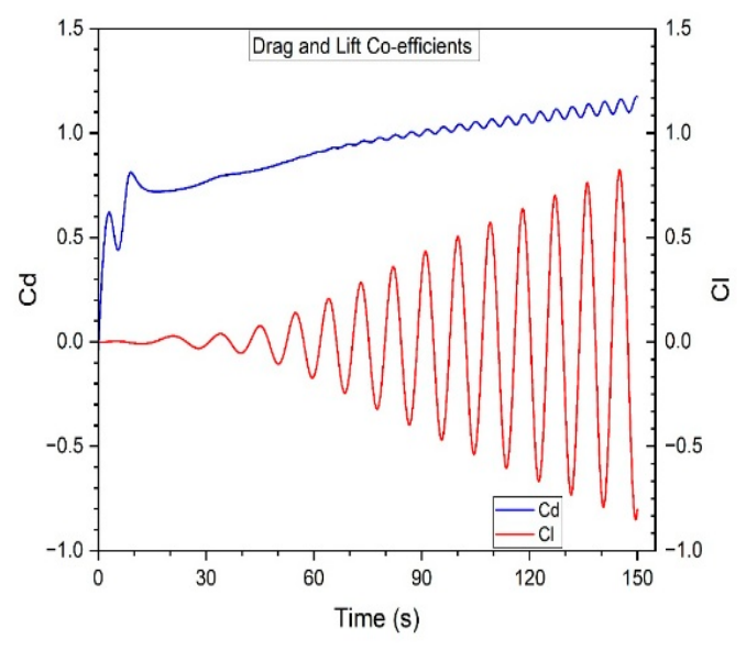
At Re=104 (Turbulent Flow): The flow is unsteady and characterized by periodic vortex shedding. The drag coefficient oscillates periodically around the mean value. As seen in Figure 10, the coefficient of drag is approximately 1.15 at t = 150s. The oscillatory component has a small amplitude, which is consistent with the expected behavior where the lift force is more significantly affected by vortex shedding as shown in Figure 12.
4.1.2. Lift Coefficient
At Re=10,000: The lift coefficient plot (Figure 11) reveals a clear, high-amplitude sinusoidal oscillation. This is the direct result of the alternating vortex shedding from the sides of the cylinder, which creates a fluctuating pressure differential. The amplitude of the lift coefficient oscillation is approximately ±0.8, indicating significant unsteady lateral forces. The periodic nature of this signal is the basis for calculating the vortex shedding frequency.
Figure 11.
Co-efficient of Lift at Re=10000.
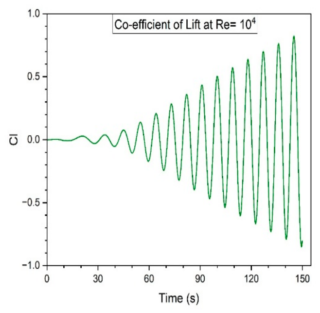
Figure 12.
Combined Drag and Lift Co-efficient vs time.
4.2. Velocity
The velocity profile for the flow was captured at different time steps from t=0.25s to 150.0s as shown in Figure 13. The velocity profiles show the transition of flow from laminar to turbulence after t=50.0s. Low velocities were recorded close to the cylinder due to the separation of flow at the wake region. Beyond the wake region, the flow begins to re-merge leading to fluctuation in the in the velocities as results. This fluctuation in velocities is because of increased turbulence. However, the velocity continues to increase in magnitude as the flow continues to lose its turbulence, becoming more stable as the flow gradually transitions back to laminar. Various probes from 1m to 20m were placed in the computational domain to measure the velocities at those points. Figure 14 and Figure 15 shows the velocities in the in the x-direction (direction of flow from inlet) and Figure 15 shows the overall magnitude of the velocity (U Magnitude)
4.3. Pressure Distribution and Fluctuations
Pressure probes were placed at several locations in the wake (x/D = 1.5, 2.5, 3.5, 5, 10, 20) to monitor the velocities at the wake region (Figure 17), the pressure field dynamics (Figure 19), and the average pressure (Figure 20).
Wake Velocity and Pressure Dynamics: The stacked pressure plots (Figure 16) clearly show the propagation of pressure fluctuations through the wake. Probe P0 (x/D=1.5), closest to the cylinder, exhibits the largest pressure fluctuations, with an amplitude of approximately ±0.6 Pa. This is directly linked to the periodic formation and convection of vortices.
Figure 16.
Propagation of pressure fluctuations through wake region.
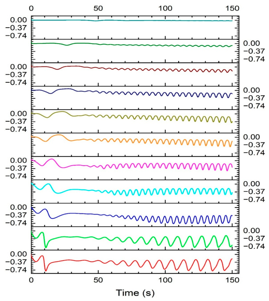
Figure 17.
Wake velocity vs streamwise position (x/D).
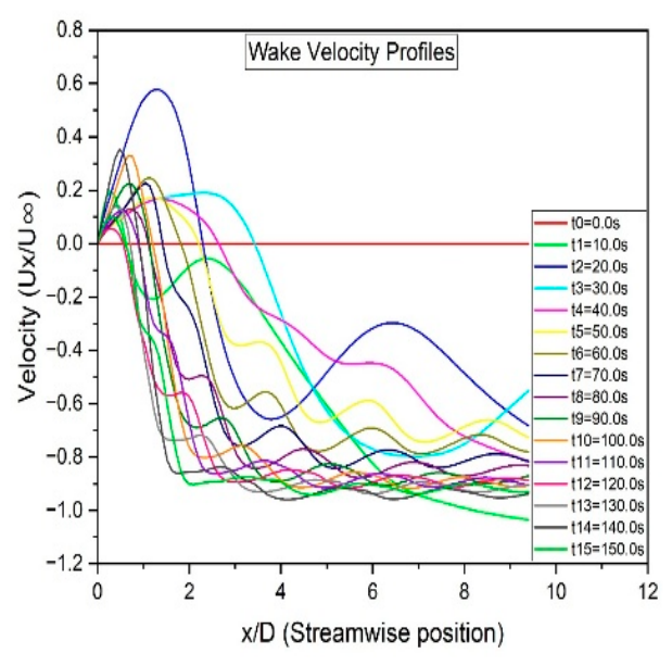
Figure 18.
Evolution of mean pressure.
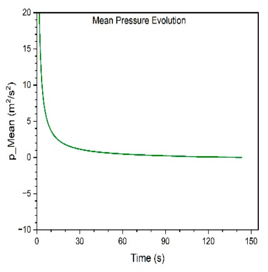
Figure 19.
Pressure evolution in wake region.
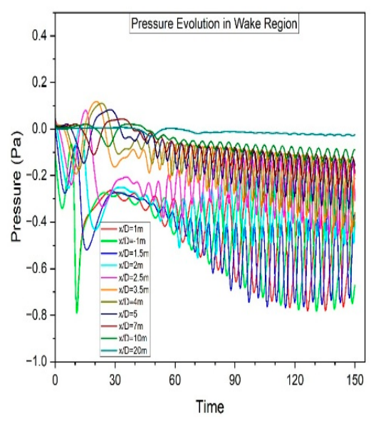
Figure 20.
Average pressure vs x/D.
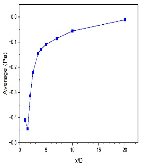
Attenuation with Distance: The amplitude of the pressure fluctuations decreases significantly with distance downstream. Probe P5 (x/D=20) shows very minor fluctuations (amplitude ~±0.03 Pa), indicating the dissipation of the coherent vortex structures far into the wake. This attenuation is characteristic of turbulent energy decay.
4.4. Wall Shear Stress
The wall shear stress components in the X and Y directions provide insight into the surface flow and separation behavior.
- Shear Stress Components: The plots of Min and Max Wall Shear Stress in X and Y directions show oscillatory behavior for Re=10,000.
- Identification of Separation Points: The periodic variation in shear stress, particularly the Y-component, is synchronized with the vortex shedding cycle. The points where the wall shear stress drops to zero indicate the instantaneous separation points on the cylinder surface. The time-averaged data from these signals was used to estimate a mean separation angle of 52.27° for laminar flow and 86.5° for subcritical from the front stagnation point, which is typical for both flow regimes as shown in Figure 21 and Figure 22 respectively.
4.5. Spectral Analysis and Strouhal Number
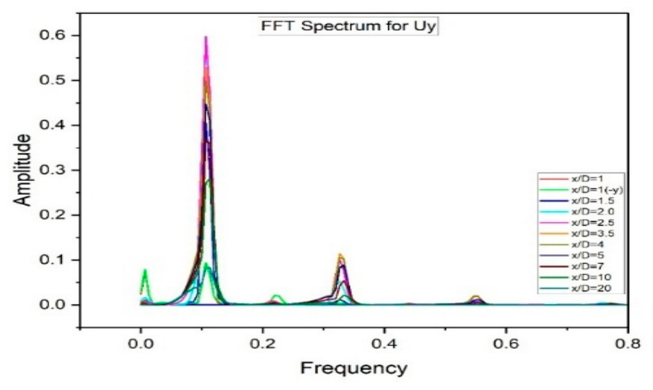
A Fast Fourier Transform (FFT) was performed on the velocity signal from a probe located in the near wake (Probe 1) to identify the dominant vortex shedding frequency.
FFT Peak and Shedding Frequency: The Spectral Analysis plots (Figure 23 and Figure 24) show a dominant, sharp peak at a specific frequency in both x and y directions. For a Reynolds number of 10,000, the Strouhal number (St) is defined as St=fD/U∞, where f is this peak frequency.
Calculation of Strouhal Number: Based on the peak frequency identified in the FFT and the given flow parameters, the calculated Strouhal number is 0.22 at x/D=2. This value aligns excellently with established empirical data and the benchmark study, providing strong validation for the model’s ability to accurately capture the unsteady wake dynamics.
4.6. Turbulent Kinetic Energy
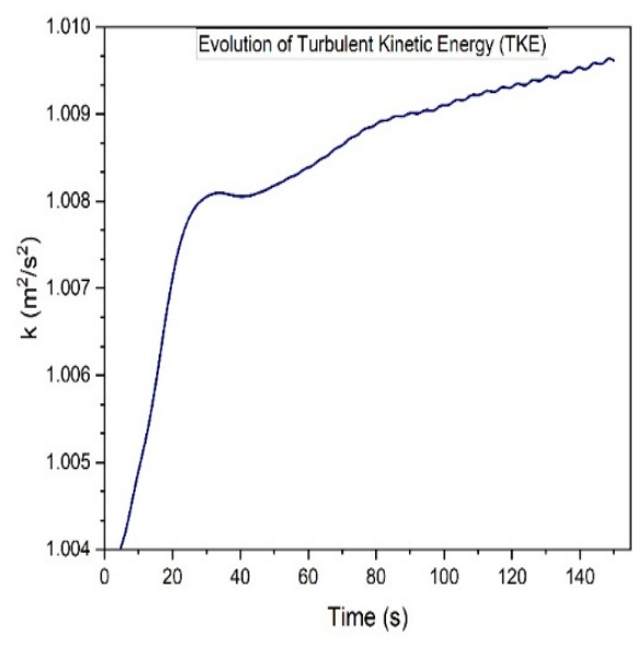
The model successfully captured the evolution of the turbulent kinetic energy in the wake region at subcritical flow regime as shown in Figure 26. This also reaffirms the model’s ability in predicting boundary layer, separation of flow, shear layers and the wake region. The evolution of TKE signifies an intense, localized turbulence generation zone. This is characteristic of a probe placed directly within the near-wake vortex formation region, immediately downstream of the cylinder. The fluctuations in the mean TKE (Figure 25) are a direct consequence of the coherent shedding; as large vortices are shed, they momentarily increase the total turbulent energy in the domain, leading to the observed fluctuations of the mean TKE.
Figure 25.
Evolution of mean TKE.
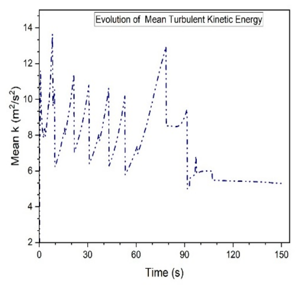
Figure 26.
Evolution of TKE.
5. Conclusions
This study validates the Unsteady Reynolds-Averaged Navier-Stokes (URANS) methodology, specifically the k-ω Shear Stress Transport (SST) turbulence model within OpenFOAM, for simulating flow around a circular cylinder—a canonical problem in fluid dynamics with direct relevance to offshore and civil engineering structures like monopiles and bridge piers. While high-fidelity simulations remain computationally prohibitive for many practical applications, URANS is an indispensable engineering tool, necessitating rigorous validation.
The study aimed to address validation gaps by not only comparing integral force coefficients but also examining derived parameters like separation angle and Strouhal number across different flow regimes. A two-dimensional computational model was developed, and simulations were conducted for laminar (Re=40) and subcritical turbulent (Re=10,000) flow. The model demonstrated excellent agreement with benchmark data. For laminar flow, the drag coefficient and separation angle matched classical results. For turbulent flow, the predicted, Strouhal number, and separation angle correlated well with established experimental and numerical studies [2,23]. Beyond force coefficients, the study provided a detailed analysis of flow development, wake dynamics, pressure fluctuation propagation, and wall shear stress, offering a holistic view of the simulated physics.
Acknowledging a primary limitation, the study notes that the 2D framework cannot capture the three-dimensional, anisotropic turbulence inherent in real-world, high-Reynolds number flows, confining direct applicability to regimes where 2D assumptions are valid. Consequently, future work should pursue full 3D simulations using URANS and Scale-Resolving Simulations (SRS) like DES or LES. The established validation protocol should be extended to a broader range of Reynolds numbers and more advanced turbulence models, ultimately facilitating integration into Fluid-Structure Interaction (FSI) frameworks for analyzing offshore infrastructure.
This study successfully validated the URANS k-ω SST model in OpenFOAM for simulating two-dimensional flow around a circular cylinder in laminar and subcritical turbulent regimes. It reinforces the model’s utility for predicting integral parameters while clearly delineating its limitations, thereby providing a clear pathway for more sophisticated and application focused research in computational marine hydrodynamics.
Data Availability Statement
The original contributions presented in this study are included in the article. Further inquiries can be directed to the corresponding authors.
Acknowledgments
Special thanks from the authors to Ghana Hydrological Authority, under the Ministry of Works, Housing and Water Resources, Ghana. This research paper is supported by funding project “National Key R&D Program of China (2023YFE0126300) and the Africa Center of Excellence in Coastal, University of Cape Coast, ACECoR, Ghana.
References
- Zdravkovich, M. M. Conceptual overview of laminar and turbulent flows past smooth and rough circular cylinders. J. Wind Eng. Ind. Aerodyn. 1990, vol. 33(no. 1–2), 53–62. [Google Scholar] [CrossRef]
- Stringer, R. M.; Zang, J.; Hillis, A. J. Unsteady RANS computations of flow around a circular cylinder for a wide range of Reynolds numbers. Ocean Eng. 2014, vol. 87, 1–9. [Google Scholar] [CrossRef]
- Pang, L. J.; Skote, M.; Lim, S. Y. Modelling high Re flow around a 2D cylindrical bluff body using the k-ω (SST) turbulence model. Prog. Comput. Fluid Dyn. An. Int. J. 2016, vol. 16(no. 1), 48–57. [Google Scholar] [CrossRef]
- He, Z.; Zhang, K.; Wang, G.; Tu, J. Vortex-induced vibration of the variable cross-sectional cylinder cases in transverse direction at Re= 3900 using OpenFOAM. Ocean Eng. 2024, vol. 303, 117511. [Google Scholar] [CrossRef]
- Jiang, C.; el Moctar, O. Numerical investigation of wave-induced loads on an offshore monopile using a viscous and a potential-flow solver. J. Ocean Eng. Mar. Energy 2022, vol. 8(no. 3), 381–397. [Google Scholar] [CrossRef]
- Padrón, L. A.; Carbonari, S.; Dezi, F.; Morici, M.; Bordón, J. D. R.; Leoni, G. Seismic response of large offshore wind turbines on monopile foundations including dynamic soil–structure interaction. Ocean Eng. 2022, vol. 257, 111653. [Google Scholar] [CrossRef]
- Achenbach, E. “Distribution of local pressure and skin friction around a circular cylinder in cross-flow up to Re= 5× 10⁶,” J. Fluid Mech. 1968, vol. 34(no. 4), 625–639. [Google Scholar] [CrossRef]
- Catalano, P.; Wang, M.; Iaccarino, G.; Moin, P. Numerical simulation of the flow around a circular cylinder at high Reynolds numbers. Int. J. Heat Fluid Flow 2003, vol. 24(no. 4), 463–469. [Google Scholar] [CrossRef]
- Rosetti, G. F.; Vaz, G.; Fujarra, A. L. C. URANS calculations for smooth circular cylinder flow in a wide range of Reynolds numbers: solution verification and validation. J. Fluids Eng. 2012, vol. 134(no. 12), 121103. [Google Scholar] [CrossRef]
- Vlastos, D.; Riziotis, V. A.; Papadakis, G.; Manolas, D. I.; Chaviaropoulos, P. K. Numerical investigation of vortex induced vibrations on cylinders. In Journal of Physics: Conference Series; IOP Publishing, 2024; p. 22034. [Google Scholar]
- Ong, M. C.; Utnes, T.; Holmedal, L. E.; Myrhaug, D.; Pettersen, B. Numerical simulation of flow around a smooth circular cylinder at very high Reynolds numbers. Mar. Struct. 2009, vol. 22(no. 2), 142–153. [Google Scholar] [CrossRef]
- Huang, L.; et al. A review on the modelling of wave-structure interactions based on OpenFOAM. OpenFOAM J. 2022, vol. 2, 116–142. [Google Scholar] [CrossRef]
- Hosur, S. M.; Ramesha, D. K.; Basu, S. Transient simulation of flow past smooth circular cylinder at very high Reynolds number using openfoam. Appl. Mech. Mater. 2014, vol. 592, 1972–1977. [Google Scholar] [CrossRef]
- Jacobsen, N. G.; Fuhrman, D. R.; Fredsøe, J. A wave generation toolbox for the open-source CFD library: OpenFoam®. Int. J. Numer. Methods Fluids 2012, vol. 70(no. 9), 1073–1088. [Google Scholar]
- Menter, F. R. Two-equation eddy-viscosity turbulence models for engineering applications. AIAA J. 1994, vol. 32(no. 8), 1598–1605. [Google Scholar] [CrossRef]
- Chen, J.; Wu, J. Numerical investigation of vortex-induced vibration of a porous-coated cylinder at subcritical Reynolds number with a combined k-ε model for porous medium. Ocean Eng. 2024, vol. 304, 117828. [Google Scholar] [CrossRef]
- Roshko. On the development of turbulent wakes from vortex streets; 1954. [Google Scholar]
- Tritton, D. J. Experiments on the flow past a circular cylinder at low Reynolds numbers. J. Fluid Mech. 1959, vol. 6(no. 4), 547–567. [Google Scholar] [CrossRef]
- Norberg, C. Fluctuating lift on a circular cylinder: review and new measurements. J. Fluids Struct. 2003, vol. 17(no. 1), 57–96. [Google Scholar] [CrossRef]
- Khan, N. B. Numerical Modeling and Analysis of Flow Around Stationary and Oscillating Circular Cylinder. In University of Malaya (Malaysia); 2018. [Google Scholar]
- Rodrıguez; Lehmkuhl, O.; Chiva, J.; Borrell, R.; Oliva, A. “Characteristics of the near wake region behind a cylinder at critical and super-critical Reynolds num-bers”. [CrossRef] [PubMed]
- Versteeg, H. K. An introduction to computational fluid dynamics the finite volume method, 2/E; Pearson Education India, 2007. [Google Scholar]
- Issa, R. I. Solution of the implicitly discretised fluid flow equations by operator-splitting. J. Comput. Phys. 1986, vol. 62(no. 1), 40–65. [Google Scholar] [CrossRef]
- Taneda, S. Experimental investigation of the wakes behind cylinders and plates at low Reynolds numbers. J. Phys. Soc. Jpn. 1956, vol. 11(no. 3), 302–307. [Google Scholar] [CrossRef]
- Coutanceau, M.; Bouard, R. Experimental determination of the main features of the viscous flow in the wake of a circular cylinder in uniform translation. Part 1. Steady flow. J. Fluid Mech. 1977, vol. 79(no. 2), 231–256. [Google Scholar] [CrossRef]
- Grove, S.; Shair, F. H.; Petersen, E. E. An experimental investigation of the steady separated flow past a circular cylinder. J. Fluid Mech. 1964, vol. 19(no. 1), 60–80. [Google Scholar] [CrossRef]
- Dehkordi, Ghadiri; Jafari, H. Houri. Numerical simulation of flow through tube bundles in in-line square and general staggered arrangements. Int. J. Numer. Methods Heat Fluid Flow 2009, vol. 19(no. 8), 1038–1062. [Google Scholar] [CrossRef]
- Park, J.; Kwon, K.; Choi, H. Numerical solutions of flow past a circular cylinder at Reynolds numbers up to 160. KSME Int. J. 1998, vol. 12(no. 6), 1200–1205. [Google Scholar] [CrossRef]
- Dennis, S. C. R.; Chang, G.-Z. Numerical solutions for steady flow past a circular cylinder at Reynolds numbers up to 100. J. Fluid Mech. 1970, vol. 42(no. 3), 471–489. [Google Scholar] [CrossRef]
- Massey, B. S. Mechanics of fluids, 6th ed.; Chapman & Hall, 1994. [Google Scholar]
- Thompson, N. Mean forces, pressures and flow field velocities for circular cylindrical structures: Single cylinder with two-dimensional flow; 1986. [Google Scholar]
- Achenbach, E.; Heinecke, E. On vortex shedding from smooth and rough cylinders in the range of Reynolds numbers 6× 10³ to 5× 10⁶. J. Fluid Mech. 1981, vol. 109, 239–251. [Google Scholar] [CrossRef]
Figure 1.
Geometry of the computed domain.
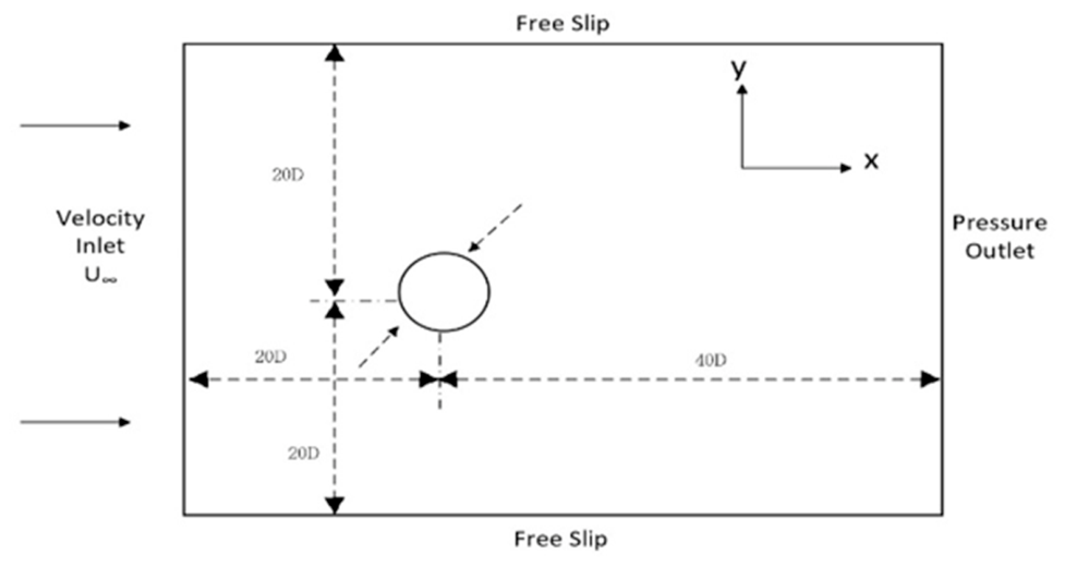
Figure 2.
refine mesh in the region adjacent to the cylinder wall.
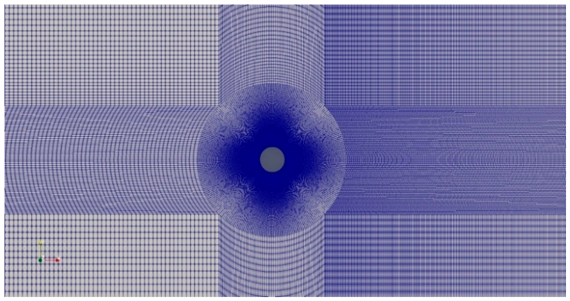
Figure 3.
refined in the wake region.
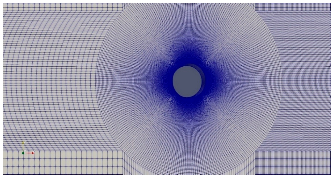
Figure 4.
Co-efficient of drag vs Reynolds number, correlation between experimental and numerical results.
Figure 4.
Co-efficient of drag vs Reynolds number, correlation between experimental and numerical results.
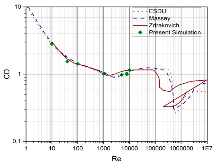
Figure 5.
Strouhal Number vs Reynolds number; correlation between experimental and numerical results.
Figure 5.
Strouhal Number vs Reynolds number; correlation between experimental and numerical results.
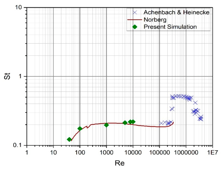
Figure 6.
Stream tracing in x-direction.
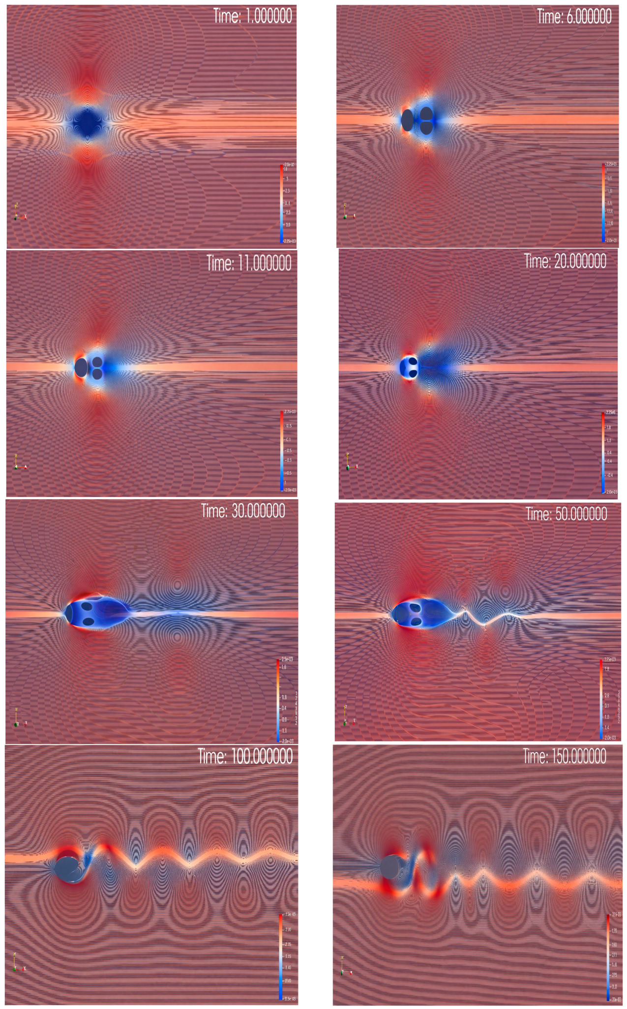
Figure 7.
Stream tracing in y-direction.
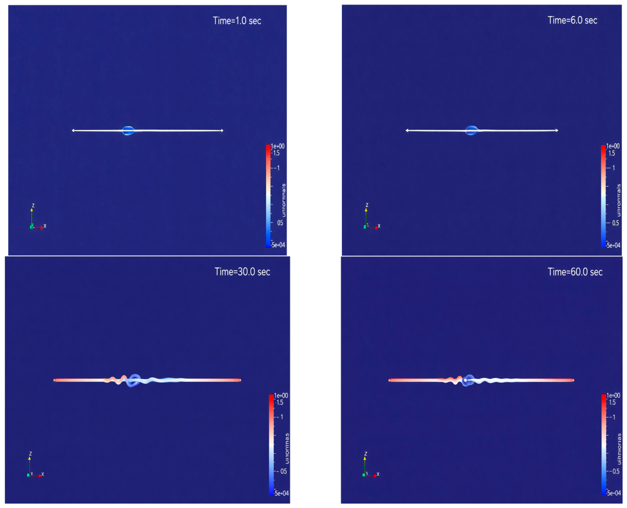
Figure 8.
Co-efficient of drag (Cd) vs Mesh Resolution.
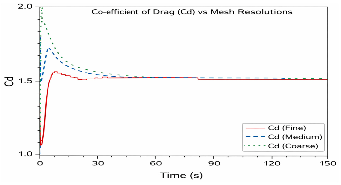
Figure 9.
Co-efficient of Lift (Cl) vs Mesh Resolution.
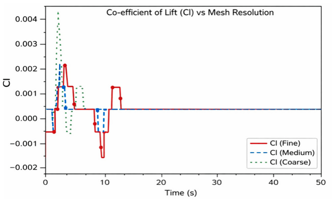
Figure 10.
Coefficient of Drag for Re=10000.
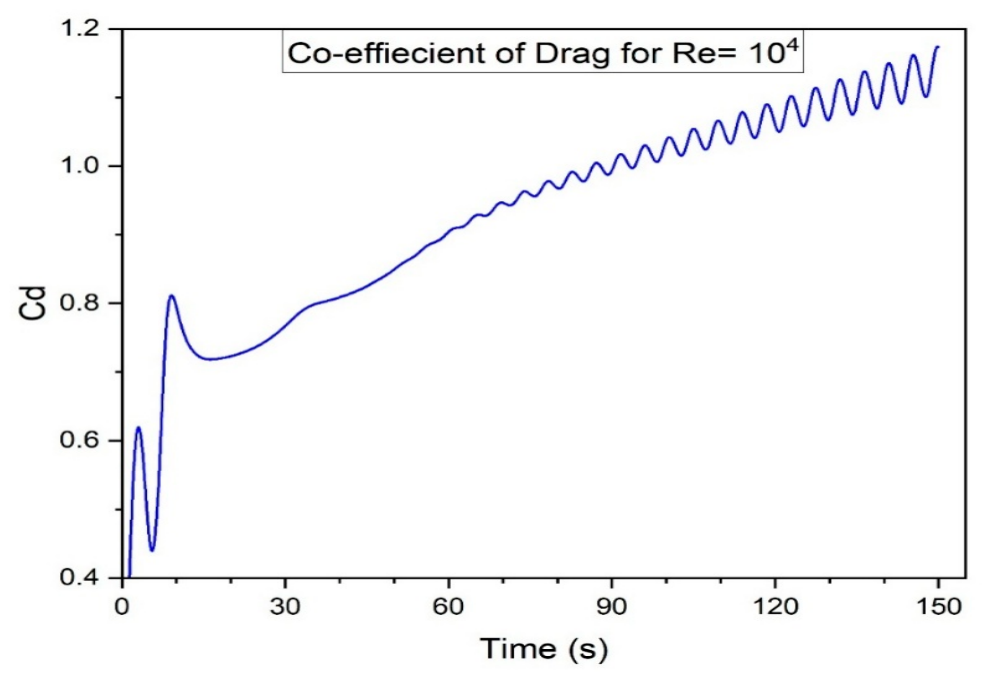
Figure 13.
Velocity profile.
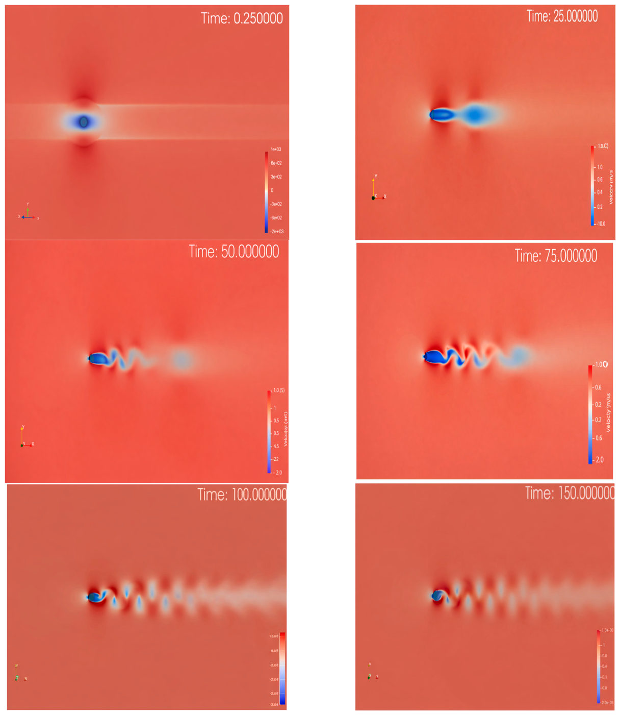
Figure 14.
Velocity Ux profiles at different probe positions.
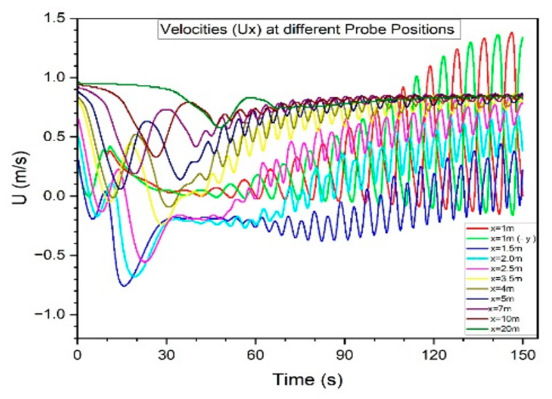
Figure 15.
Velocity |Ux| at different probe positions.
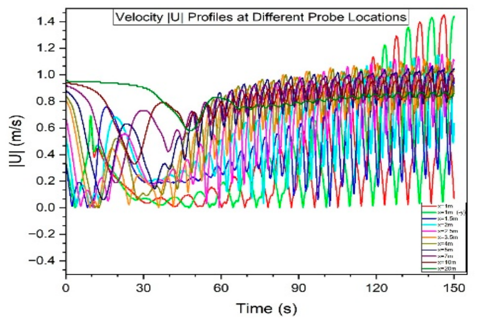
Figure 21.
Tangential velocity versus geometric angle at Re=40.
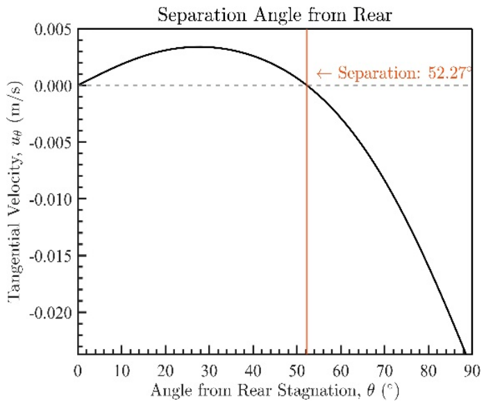
Figure 22.
Tangential velocity versus geometric angle at Re=10000.
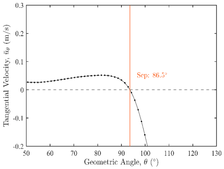
Figure 23.
FFT Spectrum for Ux.
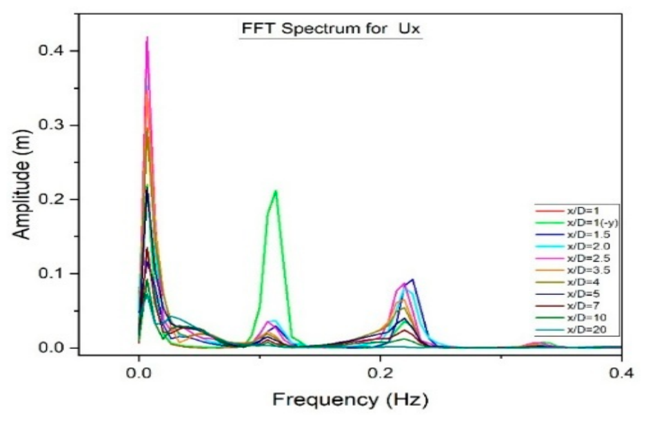
Figure 24.
FFT Spectrum for Uy.
Disclaimer/Publisher’s Note: The statements, opinions and data contained in all publications are solely those of the individual author(s) and contributor(s) and not of MDPI and/or the editor(s). MDPI and/or the editor(s) disclaim responsibility for any injury to people or property resulting from any ideas, methods, instructions or products referred to in the content. |
© 2026 by the authors. Licensee MDPI, Basel, Switzerland. This article is an open access article distributed under the terms and conditions of the Creative Commons Attribution (CC BY) license.
Copyright: This open access article is published under a Creative Commons CC BY 4.0 license, which permit the free download, distribution, and reuse, provided that the author and preprint are cited in any reuse.


