

Submitted:
11 July 2026
Posted:
13 July 2026
You are already at the latest version
Abstract
In an increasingly complex modern social information environment, in which consumers are exposed to both changes in economic conditions and pervasive social comparison cues, there remains limited research exploring the relationship between financial anticipation, social signals, and consumption choices. Using an experimental approach, we examine how income trajectories and social information shape consumption choices. Participants in our online decision task were randomly exposed to information indicating either increasing or decreasing income trajectories, alongside social information about the popularity of a relatively cheap or expensive choice of a specific type of product, among individuals with the same income trajectory. Firstly, we find that cheap information during economic decline undermines the standard prediction that anticipated income decline leads consumers to prefer cheaper products. Specifically, the results indicate a significant non-conformity effect specific to the scenario of anticipated income decline: when income was expected to decrease and the social information indicated a majority choice of cheap products, participants were more likely to select the expensive products. On the other hand, social information had no significant impacts when income was expected to increase. Our findings challenge the conventional intuition of a socially-driven trend in frugal consumption, highlighting counter-conformity as a driver of expensive purchase behavior during economic downturns.
Keywords:
income anticipation
; social information
; counter-conformity
; consumption behavior
; cheap-salience
1. Introduction
In modern economic systems, individual decision-making is often constrained by dual frictions: aggregate fluctuations in the economic environment and peer effects within the social information landscape. As global economic uncertainty becomes normalized, consumers face not only idiosyncratic shocks to future income streams but also reside within a highly transparent network of social comparison. This has heightened the salience of income trajectories and social comparison in everyday consumption choices. These forces raise a fundamental question: how do consumers integrate anticipations about their future income with social information when choosing between cheap and expensive products?
Standard consumption theory predicts that anticipated income declines should strengthen preferences for cheaper goods through precautionary saving and tighter budget constraints [1]. At the same time, a large body of empirical evidence documents that social information (e.g., what others choose) systematically shapes individual behavior [2]. However, how these two forces interact remains insufficiently understood, particularly in environments characterized by economic pressures and different income trajectories.
This study employs a randomized controlled experiment to identify the mechanisms of consumption choice under economic pressure by exogenously manipulating income trajectories and social information. Within a described context of economic downturn and unstable employment, participants were exposed to social information indicating whether the majority or minority chose the cheaper or more expensive option among two products. The study’s core finding reveals a counter-intuitive “non-conformity effect”: in the treatment group under income decline, when the social information was “cheap-preferring,” the probability of participants selecting expensive products significantly increased. This suggests that during economic downturns, social information about cheaper choices may in fact fail to induce frugality and instead act as a psychological threat, triggering consumers to engage in counter-conformity via expensive purchases as a possible channel for avoiding social status devaluation.
A large literature in microeconomics and behavioral economics studies how information affects consumption choices. Early work emphasized expectations about lifetime income as a key determinant of consumption smoothing [1]. More recent studies highlight the role of economic uncertainty and pessimistic income trajectories in shaping precautionary behavior [3,4]. These studies consistently predict reduced demand for expensive goods when income prospects deteriorate.
Another strand of literature documents that economically equivalent information can lead to systematically different choices depending on how information is framed [5]. In consumption contexts, price and reference points have been shown to influence demand, perceived value, and willingness to pay [6]. However, asset price expectations yield heterogeneous effects: while renters reduce spending when anticipating higher home prices due to housing cost burdens, homeowners’ spending remains unaffected, reflecting wealth offsetting [7]. This highlights how economic constraints and identity-based motivations can interact with information to shape consumption decisions.
A growing literature emphasizes the influence of social information and peer effects on economic behavior [2]. Information about majority choices often induces conformity, especially under uncertainty [8]. However, recent work also suggests that social signals can also generate a deviation from the conformity when status or identity concerns are salient [9,10]. Under situations of increasing or decreasing income trajectories, an individual’s income trend or economic condition can serve as an identity factor which influences conformity and a deviation from the conformity behavior. Our experiment enables a systematic examination of the impacts of the observable choices of others on individual’s own consumption choice under a shared income trajectory.
This issue is of particular importance in addressing questions of whether economic downturns inevitably lead to a perpetual spiral of ‘downgraded’ consumption, or whether there are fundamental counteracting forces at the microeconomic and psychological level, which can naturally mitigate such undesirable macroeconomic outcomes. The results in our study suggest that perhaps societies need not be overly concerned about endless cycles of downgraded consumption. The reason is that consumers may naturally gravitate towards a tendency to distinguish themselves from their peers in the same income trajectory group, by choosing more expensive products when their peers choose cheaper products. However, this finding also bears a cautionary message in terms of the consumer welfare of consumption choices, in that the tendency to gravitate towards more expensive options from a social status motive can exert additional economic pressures on consumers during periods of income decline.
The remainder of this paper proceeds as follows. Section 2 describes conceptual framework and hypotheses. Section 3 introduces the detailed study design and implementation procedure. Section 4 presents the main results and robustness checks, along with heterogeneity analysis. Section 5 concludes and discusses policy implications.
2. Conceptual Framework and Hypotheses
Recent research emphasizes that consumption responses to income trajectories depend critically on perceived economic security rather than expected income levels alone. Empirical evidence indicates that reference dependence can shape dynamic decisions under uncertainty [11]. Evidence from high-frequency administrative and survey data shows that households exposed to negative income news sharply reduce discretionary spending, consistent with heightened consumption discipline rather than smooth adjustment of consumption [12]. Related work further documents that perceived labor market fragility amplifies conservative consumption behavior even in the absence of realized income losses [13]. In this context, an anticipated income decline reduces the effective consumption constraints and increases sensitivity to price-related considerations, thus, consumers facing pessimistic income trajectories should be expected to display stronger preferences for cheaper options.
A growing literature indicates that social information functions as a significant behavioral influence when individuals face uncertainty and limited confidence in their private assessments. Empirical evidence indicates that households systematically update beliefs and economic plans in response to socially transmitted narratives, even when such narratives are only loosely connected to fundamentals [14]. In consumption contexts, information about majority choices can therefore serve as a coordination device, reducing perceived decision risk and cognitive effort. This role of social information is expected to intensify when economic prospects deteriorate. Anticipated income decline increases uncertainty about future resources, making individuals more reliant on external information such as majority behavior.
Beyond the informational content of social signals, framing can further shape how economic information is interpreted. Experimental and field evidence suggests that labels emphasizing prudence or thrift can alter preferences by changing the perceived appropriateness of behavior, even when objective trade-offs remain unchanged [15]. In economic downturn environments, the majority behavior of cheap may highlight prudence, self-control and economic rationality. It can legitimize frugal consumption and amplify conformist responses among individuals who perceive cheap choices as socially appropriate under economic pressures.
Economic pressure may simultaneously heighten sensitivity to social rank and identity concerns. Recent research shows that perceived downward mobility risk can trigger compensatory behavior aimed at preserving one’s social standing [16]. Related evidence demonstrates that threats to self-image induce compensatory actions that are often costly in material terms [17]. Applied to consumption choices, when cheap options become socially associated with vulnerability or decline, individuals may deliberately deviate from the cheap-majority consumption pattern. In such contexts, choosing expensive products can function as a costly signal of resilience, self-worth or social distinction.
When an individual’s income is expected to increase, economic uncertainty is relatively low and perceived budget constraints are relaxed. Under such conditions, individuals are less dependent on external social cues and more likely to rely on stable preferences or intrinsic product valuation. [14] found support for this, which suggests that the behavioral influence of social information weakens when decision-makers feel economically secure. Therefore, the majority choice was cheap or expensive should not systematically affect consumption decisions when income prospects are favorable.
With these concepts and theories, we formulate the following hypotheses about the relationship between income trajectories, social information and the choices of cheaper products. Our information disclosure treatments and subsequent statistical analysis will shed light on whether there are differences in conformity behavior across income trajectories conditions, and whether information about others’ choices of cheap salient products versus expensive salient products accounts for these patterns in meaningful ways:
Our first hypothesis addresses the general pattern of product purchase between anticipated income decrease versus increase.
Hypothesis 1: Decision-makers under anticipated income decline choose cheap products more frequently than those anticipating income increase.
This hypothesis straightforwardly reflects the notion that consumers under expected income decrease gravitate towards cheaper products. The reasoning is that given that when income is expected to decline, individuals face heightened economic insecurity and increased concern over future resources. Standard economic reasoning predicts that such conditions strengthen consumption discipline and amplify price sensitivity. This income-driven preference for cheaper options should manifest as a baseline pattern, regardless of whether social information is available.
Our second hypothesis addresses product choices under income decline, specifically whether consumers tend to conform to majority choices or not. While Hypothesis 1 predicts a general shift toward cheaper products under income decline, social information may trigger more complex responses when frugal consumption is socially salient. Based on the literature on social information and influence, we expect social information to suggest conformity effects. Building on this foundation, Hypothesis 2 examines how social information affects cheap product consumption under anticipated income decline. However, at a more granular level, we recognize that two competing mechanisms may be at play:
Hypothesis 2A1 (Conformity to Frugal Patterns): Social information indicating that the majority of consumers facing the same anticipated income trajectory chose cheap products will reinforce frugal consumption patterns.
This hypothesis posits that social information serve a dual function as both informational guidance and social justification, strengthening the normative pull toward prudent consumption and conferring legitimacy on frugal choices. Consequently, individuals will conform to the frugal majority.
Alternative mechanism (Counter-Conformity): Economic decline may threaten individuals’ perceived social status and self-image. When cheap consumption becomes socially salient through information about majority purchases, it may signal overall vulnerability or downward mobility among those facing anticipated income decline. In response, individuals may be motivated to specifically avoid conforming to the majority choice. One explanation is that information about majority cheap purchases triggers a costly counter-conformity motive, whereby individuals attempt to achieve social distinction and resist association with the economically constrained group.
Hypothesis 2A2 (Social Information and Counter-Conformity): Under anticipated income decline, individuals exposed to social information, particularly for the cheap-majority information will choose cheap products less frequently than those receiving no information, thus exhibiting counter-conformity.
Social Information Moderates the Income-Conformity Relationship
While the previous hypotheses specify how the purchase of differently priced products depend on expected income trends (income decrease, specifically), and potentially on social information, our next set of hypotheses specifically addresses the relationship between conformity and income trajectories. We define conformity in this context as choosing the product that the majority of consumers chose, based on the social information provided to the decision-maker.
However, we note that our experiment design has a limited capacity to uncover a broad relationship between conformity and income trajectory. The reason is that due to the methodology of experimental economics social information about consumption choices were derived from actual pilot data; in the pilot data income-declining participants (who tended to prefer cheap products, consistently with Hypothesis 1) disproportionately received “cheap-majority” information. Thus, observed “conformity” could reflect either genuine social influence, or underlying preferences.
Hypothesis 3: Income-declining individuals exhibit higher conformity than those in income-increasing individuals (baseline, potentially confounded).
Once cheap salience information is accounted for, the conformity gap may disappear if the observed difference in Hypothesis 3 is driven by preference rather than genuine social influence.
Hypothesis 4: Once cheap salience information is accounted for, the conformity gap between income-declining and income-increasing individuals disappears.
Separately, Hypotheses 4A1 and 4A2 address the independent effect of cheap-salience information on conformity. These are directional alternatives: cheap-salience information may either reinforce conformity by signaling that the majority chose the budget option, or suppress it by triggering reactance or signaling low social status.
Hypothesis 4A1: Cheap salience information positively predicts conformity.
Hypothesis 4A2: Cheap salience information negatively predicts conformity.
Information Effects under Income Increase
Hypothesis 5 examines how social information shapes product choice for income-increasing individuals. When income is anticipated to increase, economic uncertainty is relatively low and perceived budget constraints are relaxed, making individuals less reliant on external social cues. Hypothesis 5 therefore serves as a general null hypothesis against the no-information baseline.
Hypothesis 5: When income is anticipated to increase, social information, whether cheap or expensive salience, has no systematic effect on product choices relative to the no-information baseline.
Building on Hypothesis 5, Hypothesis 6 examines a more specific directional question: whether the form of information presentation within the information-present conditions produces differential responses, independent of the overall null effect relative to no information.
Hypothesis 6: Among individuals facing income increase, being informed that fewer people chose the expensive option (minority-expensive information) will lead to more frequent cheap product choices compared to being informed that the majority chose the cheap option (majority-cheap information).
3. Study Design
3.1. Experimental Design
We employed a 2×2 between-subjects design to examine how income trajectory and social consumption information, influence consumption choices. The two core factors were income conditions (increasing vs. decreasing) and information salience (displaying cheap-product choice proportions vs. expensive-product choice proportions).
To establish proper baselines, we included two control groups that received no social consumption information— one for each income condition. Combined with the four treatment conditions that varied both income anticipation and information salience, this resulted in six experimental conditions total. A total of 480 participants were recruited via the online platform Credamo and initially assigned randomly to one of the six conditions ( per condition), resulting in a final valid analytical sample of 468 participants. The study took approximately 5 minutes for subjects to complete. 1
It is important to clarify the structure of the social information manipulation. The between-subject treatment is the information salience framework: whether the proportion choosing the cheap product (Cheap Salience: Treatment C1, Treatment C2) or the proportion choosing the expensive product (Expensive Salience: Treatment c11, Treatment c22) is displayed. Because all information derived from actual pilot data rather than constructed percentages, the majority or minority status of each product’s choice varies naturally across the 10 products within each condition. To most directly test the theoretical predictions of counter-conformity under economic strain, our primary analyses focus on the comparison between the no-information baseline and the social information treatment within the income-decline trajectory.
3.2. Social Information Construction
The pilot study was conducted on February 10, 2025, with 30 participants per income condition2. Based on these data from actual choices from the same product choice sets, we created two types of information salience treatments:
Cheap Salience Treatment: Participants viewed information about the proportion of people who chose the cheap product.
Expensive Salience Treatment: Participants viewed information about the proportion of people who chose the expensive product.
Note that these two treatments are merely different presentations of the same underlying choice data. The treatment lies in which product type’s selection proportion is displayed, but not in altering actual majority/minority relationships.
Note that pilot participants in different income conditions exhibited different product preferences, the information distribution differed across income conditions:
Income-increasing conditions: Across 10 product pairs, the cheap salience treatment displayed cheap-product selection proportions for 4 items (Q3, Q4, Q8, Q12), while the expensive salience treatment displayed expensive-product selection proportions for 6 items (Q5, Q6, Q7, Q9, Q10, Q11).
Income-decreasing conditions: Across 10 product pairs, the cheap salience treatment displayed cheap-product selection proportions for 9 items (Q3, Q4, Q5, Q6, Q7, Q8, Q10, Q11, Q12), while the expensive salience treatment displayed expensive-product selection proportions for 1 item (Q9).
Control groups received consumption pairs but no information regarding others’ choices, serving as the reference group for identifying social information effects. A detailed outline of the different treatment groups is provided in Figure 1.
3.3. Experimental Procedure
The experimental procedure was conducted online using the platform Credamo. After providing informed consent and reading task instructions, participants were exposed to the income trajectory condition. To enhance psychological engagement with the scenario, participants were asked to imagine themselves in a specific economic situation. They read a detailed textual scenario describing either declining or rising income anticipations, accompanied by a simulated bar graph visualizing the income trajectory over time. In the income-decreasing condition, the scenario described economic downturn, industry-wide decline, and job instability as factors causing continuous income decline. In the income-increasing condition, participants read a parallel scenario depicting positive economic outlook, industry growth, and stable career advancement leading to rising income. This imaginative scenario was designed to create stronger immersion, making the scenario more convincing.
To ensure participants thoroughly processed the scenario and actively engaged with the imagined situation, they were asked two engagement questions (Q1 and Q2) about the hypothetical scenario’s impacts on their lives. These questions encouraged participants to think realistically about the scenario and adopt the corresponding mentality, thus deepening engagement with the treatment. Following this, participants completed an ordinary attention check that instructed them to select a specific option to verify attentive participation. Participants who failed this check were terminated from the survey.
Our study employs a scenario-based vignette design: a detailed written description of an economic situation accompanied by a visualized income trajectory graph. Vignette-based experiments have been widely validated as a method for inducing hypothetical economic states. Hainmueller et al. [18] demonstrated that responses to carefully constructed vignettes closely predict real-world behavior, and Aguinis and Bradley [19] provide methodological best-practice guidance confirming the validity of vignette designs for causal inference in behavioral research. To ensure that participants genuinely adopted the intended income mindset rather than passively reading the scenario, we included two post-scenario engagement questions: participants rated their satisfaction with the imagined income trajectory (Q1, 9-point Likert scale) and identified the anticipated life impacts of the income change (Q2, multiple choice). As expected, income-decrease participants reported significantly lower satisfaction than income-increase participants ( vs. , , ), and selected negative life impacts (e.g., reduced financial security, lower consumption) at significantly higher rates. These results confirm that the scenario successfully induced the intended differential mindset across conditions.
Participants then engaged in the main consumption choice task (Questions 3–12), selecting from 10 pairs of consumption goods across various categories (fruits, beverages, shoes, hats, etc.; see Table 1). Figure 2 illustrates the visual presentation with example product pairs. Panel A (left): Cheap salience treatment showing the percentage who chose cheap products (Q3: 66.7% chose the cheaper beverage at ¥13.9; Q4: 60% chose the plain cap at ¥37). Panel B (right): Expensive salience treatment showing the percentage who chose expensive products (Q3: 33.3% chose the premium beverage at ¥33; Q4: 40% chose the Yankees cap at ¥227). These two panels illustrate complementary information of the same underlying choice data. Control group participants saw identical product images and prices but without percentage information. In all displays, the left column presented cheap products, while the right column presented expensive products (see Figure 2; Note on Imagery: To comply with copyright regulations, the original images from the experiment have been replaced here with photos of identical angle, composition and layout taken directly by the authors). Table 1 provides the complete list of all product pairs used in the study (see Table 1).
Before making choices, participants received instructions clarifying that: (1) their anticipated income allowed them to purchase any displayed product, and (2) images and prices were for reference only, their choices represented preferences for similar products at similar price points, not necessarily the exact items shown. This disclaimer ensured choices reflected price-tier preferences rather than specific brand features.
Treatment group participants received additional information stating that the displayed choice percentages came from other participants facing the same income trajectory and could serve as a reference for decision-making. Participants were also informed that these percentages were obtained from a different participant pool and therefore might not fully correspond to the choices made in their own session. This was intended to ensure that the information was perceived as a reference signal rather than a deterministic forecast of others’ behavior. Depending on condition assignment, participants saw either the percentage who chose the cheap product (left column) or the percentage who chose the expensive product (right column). These percentages derived from actual pilot study data. Control group participants saw only the product pairs without any social information.
The study concluded with a post-task questionnaire covering demographics (age, gender, education), actual wealth conditions (monthly income, residence type), and perceptions about future economic growth.
Consumption choices were hypothetical and not financially incentivized. Participants received a fixed payment upon completion regardless of their choices. This design was adopted because the study focused on consumption decisions under hypothetical income trajectories and sought to incorporate a broad range of products and price points (from ¥13.9 to ¥7,199). This choice of stimuli was intentionally designed to reflect a wide range of commodity prices and item categories in the study; however, this wide distribution precluded the practical implementation of real consumption in the experiment. Accordingly, participants made hypothetical consumption choices, reflecting a common practice in consumer behavior and psychology experiments where practical constraints often prevent the use of real consumption decisions. Prior research has shown that such hypothetical choice paradigms can provide meaningful insights into consumer preferences and decision-making under hypothetical economic scenarios [20,21].

Table 1.
Product Pairs and Pilot Selection Percentages.
| Income Decrease | Income Increase | ||||||
|---|---|---|---|---|---|---|---|
| Q# | Category | Cheap (Price) | Expensive (Price) | Cheap% | Expensive% | Cheap% | Expensive % |
| Q3 | Beverage | Domestic chain (¥13.9) | International chain (¥33) | 100.0 | 0.0 | 66.7 | 33.3 |
| Q4 | Hat | Basic (¥37) | Branded (¥227) | 86.7 | 13.3 | 60.0 | 40.0 |
| Q5 | Shoes | Standard (¥99) | Premium (¥799) | 76.7 | 23.3 | 46.7 | 53.3 |
| Q6 | Meal | Box meal (¥15) | Stir-fry (¥27) | 56.7 | 43.3 | 26.7 | 73.3 |
| Q7 | Fruit | Loose (¥15) | Premium (¥45) | 83.3 | 16.7 | 43.3 | 56.7 |
| Q8 | Sports | Basic racket (¥114) | Carbon (¥560) | 86.7 | 13.3 | 66.7 | 33.3 |
| Q9 | Cup | Practical (¥20) | Premium (¥84) | 46.7 | 53.3 | 16.7 | 83.3 |
| Q10 | Shampoo | Basic (¥39) | Functional (¥120) | 63.3 | 36.7 | 23.3 | 76.7 |
| Q11 | Skincare | Basic (¥122) | Premium (¥530) | 70.0 | 30.0 | 33.3 | 66.7 |
| Q12 | Phone | Domestic (¥4,775) | International (¥7,199) | 86.7 | 13.3 | 70.0 | 30.0 |
4. Main Results
Table 2 provides a complete overview of cheap product choices across all six experimental conditions. To facilitate direct comparison across subsequent analyses, we present both the full 10-product totals and the 9-product totals with Q9 excluded. This exclusion reflects a specific empirical pattern observed in our pilot data: under the income-decrease trajectory, Q9 was the only product for which the majority of pilot participants chose the expensive option. As such, Q9 represents an isolated anomaly rather than a systematic tendency, and its inclusion would introduce noise into aggregate comparisons. Excluding Q9 therefore yields a cleaner baseline for comparing the social information treatment against the no-information control group under the income-decrease trajectory. We refer to this 9-product sample as the analytical sample throughout the remainder of the paper.
4.1. Income Changes and Product Choice Patterns
We first examine whether income trajectory fundamentally shapes product preferences. All statistical tests reported in this section and throughout Section 4 are two-sample proportion tests. Corresponding robustness checks using independent-samples t-tests on participant-level means are provided in Appendix A, yielding substantively identical results.
Results confirm that individuals anticipating income decline choose cheap products significantly more frequently than those anticipating income increase, supporting Hypothesis 1 (See Figure 3). In the no-information condition, the proportion of cheap product choices was 0.766 for income-declining participants in Treatment A2 compared to 0.440 for income-increasing participants in Treatment A1 (). In the social information condition, the proportion was 0.702 for income-declining participants in the combined Treatment C2/c22 compared to 0.463 for income-increasing participants in the combined Treatment C1/c11 ().
The gap between income-declining and income-increasing groups narrows slightly in the information-present condition (0.702 − 0.463 = 0.239) relative to the no-information baseline (0.766 − 0.440 = 0.326). Notably, this aggregate pattern shows important heterogeneity. The observed difference was largely concentrated among those receiving the social information, particularly for the cheap-majority information. This indicates a complex interaction between income trajectories and the social information, which we examine in subsequent analyses (Section 4.2 and Section 4.3).
4.2. Social Information Effects: Evidence of Counter-Conformity
4.2.1. Basic Statistical Tests
To test whether individuals under income-decline show a conformity or a counter-conformity pattern when exposed to social information (Hypothesis 2), we conducted statistical tests of proportions comparing cheap product selection rates between the no-information condition and the social information conditions within the income-decline group.
Our primary analysis included all conditions within the analytic sample where participants were exposed to social information — encompassing both cheap-salience (Treatment C2) and expensive-salience (Treatment c22) conditions. As shown in Figure 4, the aggregate result is highly significant: participants exposed to social information selected cheap products significantly less frequently than those receiving no information ( vs. ; ), providing strong support for the counter-conformity hypothesis.
We further restrict the comparison to the cheap-salience condition alone (Treatment A2 vs. Treatment C2) to examine which component of social information drives this effect. As shown in Figure 5, the counter-conformity pattern remains highly significant in this restricted sample, suggesting that it is primarily the cheap-majority information that drives the aggregate result. Note that the baseline proportion for the no-information group is identical to that reported in Figure 4 (0.786), as both analyses use Treatment A2 as the reference.
The results suggest that income-declining participants exposed to social information consistently chose expensive products more frequently than the no-information group, supporting Hypothesis 2A2. This finding is particularly striking given the economic context: individuals already facing income decline are, upon receiving social information, further nudged toward more expensive consumption choices. Rather than reinforcing financially prudent behavior, social information appears to trigger a counter-conformity response that may exacerbate financial vulnerability.
One plausible explanation is that exposure to social information triggers a pattern primarily driven by status signaling and self-concept protection. Faced with a perceived threat to their economic identity, these individuals may engage in compensatory consumption, choosing expensive products to signal financial resilience and distance themselves from the “frugal majority” [22]. By actively rejecting choices that align with their objective financial decline, they protect their self-concept from the negative connotations associated with economic constraint. This dynamic is further supported by evidence that consumer behavior is not solely driven by personal income but also by aspirational alignment with higher-status groups [23].
Furthermore, this behavior may partly stem from hedonic compensation triggered by economic anxiety. Research shows that economic anxiety heightens reliance on hedonic purchases for emotional regulation [24], and present-biased preferences are amplified under financial stress [25]. Additionally, sensitivity to social comparison may spark psychological reactance: individuals may reject inexpensive options to avoid being categorized with a struggling peer group, consistent with findings that economic inequality shapes how individuals perceive their place in the social hierarchy [26].
4.2.2. Tobit Regression Analysis
To validate the counter-conformity pattern using a more rigorous analytical framework, we estimated a two-limit Tobit model within the analytic sample, setting a lower bound at 0 and an upper bound at 9. The dependent variable is the total number of cheap products chosen out of 9 eligible product pairs (bounded integer, range 0–9). While the bounds reflect experimental design rather than data censoring in the strict econometric sense, the two-limit Tobit model is a standard approach for bounded count outcomes of this type. Standard errors are clustered at the participant level to account for within-person correlation across the 9 product choices. Following our primary analysis, we compared the cheap-salience group exposed to cheap-majority information against the no-information baseline within the income-decline condition.
Results confirmed the counter-conformity effect. Exposure to social information, specifically for the cheap-majority information, significantly reduced cheap product selection, especially after controlling for demographic characteristics (gender and age). This negative association remained robust across model specifications, providing additional confidence in our findings.
The Tobit model also included participants’ perceptions of future economic growth as control variables, which served to validate our income condition. Compared to neutral expectations, very pessimistic economic outlooks significantly increased cheap product selection, while very optimistic outlooks significantly decreased it. These patterns confirm that subjective economic perceptions operate similarly to our experimental income trajectory condition.
Table 3.
Tobit Regression - Counter-Conformity Effect in Income-Decrease Group.
| VARIABLES | (1) | (2) | (3) | (4) | (5) |
|---|---|---|---|---|---|
| Cheap Choice | Cheap Choice | Cheap Choice | Cheap Choice | Cheap Choice | |
| Cheap Majority Information | -0.779* | -0.748* | -0.921** | -0.829* | -0.885** |
| (0.455) | (0.454) | (0.445) | (0.434) | (0.429) | |
| Economic Outlook: | |||||
| Very Pessimistic | 3.521** | ||||
| (1.670) | |||||
| Pessimistic | -0.196 | ||||
| (0.736) | |||||
| Slightly Pessimistic | -0.362 | ||||
| (0.618) | |||||
| Slightly Optimistic | -0.587 | ||||
| (0.678) | |||||
| Optimistic | -2.275* | ||||
| (1.287) | |||||
| Very Optimistic | -3.532*** | ||||
| (0.894) | |||||
| Constant | 7.621*** | 8.176*** | 7.936*** | 8.657*** | 10.635*** |
| (0.323) | (0.486) | (0.594) | (1.228) | (1.873) | |
| Controls Included | |||||
| Female | No | Yes | Yes | Yes | Yes |
| Age | No | No | Yes | Yes | Yes |
| Income | No | No | No | Yes | Yes |
| Residence | No | No | No | Yes | Yes |
| Education | No | No | No | No | Yes |
| Observations | 1,413 | 1,413 | 1,413 | 1,413 | 1,413 |
| Log-likelihood | −2833.66 | −2824.28 | −2797.87 | −2764.46 | −2672.88 |
| AIC | 5673.31 | 5656.56 | 5611.75 | 5564.92 | 5399.76 |
| McFadden | 0.005 | 0.008 | 0.017 | 0.029 | 0.061 |
Standard errors clustered at participant level in parentheses; *** p<0.01, ** p<0.05, * p<0.1. Notes: Within the analytical sample, the dependent variable is the total number of cheap products chosen out of 9 eligible product pairs (bounded integer, range 0–9). A two-limit Tobit model is employed with lower bound at 0 and upper bound at 9. Sample restricted to the income-decrease condition (Treatment A2: no information vs. Treatment C2: cheap-salience information). With 157 participants (79 in Treatment A2, 78 in Treatment C2) × 9 product choices = 1,413 question-level observations. Treatment c22 (expensive-salience, income-decreasing) is excluded as the primary comparison of interest is the effect of cheap-majority social information relative to no information. The reference category for treatment is “No Information”; The reference category for economic outlook is “Neutral”.
4.2.3. Effects of Social Information under Economic Growth
The findings above demonstrate a clear counter-conformity effect during economic downturns, when informed that the majority chooses cheaper products, individuals respond by increasing their selection of expensive alternatives. By contrast, in the economic growth condition, we first examine whether social information overall has any effect relative to the no-information baseline. Comparing Treatment A1 (no information) against the combined social information Treatment C1/c11, the proportion of cheap product choices does not differ significantly (0.613 vs. 0.646, ), confirming that social information as a whole has no significant effect under income increase. Similarly, restricting to the cheap-majority information only, the proportion of cheap choices does not differ significantly between Treatment A1 and Treatment C1 (0.613 vs. 0.607, ). These results are consistent with Hypothesis 5.
Therefore, the more relevant question in this context is whether the form of social information presentation produces differential responses within the information-present conditions. Specifically, we compare two forms of information: one emphasizing that “the majority chooses cheaper products” (Treatment C1), and the other emphasizing that “fewer people choose the expensive option” (Treatment c11). The results show that exposure to minority-expensive information leads to a significantly higher proportion of cheap product choices compared to cheap-majority information (0.685 vs. 0.607, one-tailed, two-tailed), supporting Hypothesis 6. Figure 6 shows that under an expected income increase, exposure to minority-expensive information elicits a stronger preference for cheap products than exposure to majority-cheap information (See Figure 6).
For consistency with the income-decreasing analysis, we also examine whether the difference in information presentation between cheap-salience (Treatment C2) and expensive-salience (Treatment c22) produces differential responses under income decline. The proportion of cheap product choices does not differ significantly between Treatment C2 and Treatment c22 (0.718 vs. 0.740, ), suggesting that the differential response to information presentation observed under income increase does not generalize to the income-decreasing condition.
4.3. Role of Information
4.3.1. Baseline Conformity: Income Decline vs. Income Increase
To test whether income-declining individuals exhibit higher baseline conformity than income-rising individuals (Hypothesis 3), we estimated logistic regression models using conformity (coded 1 if participants chose the majority option, 0 otherwise) as the dependent variable. We restricted this analysis to the information-present conditions to isolate the effect of income trajectories on susceptibility to social influence.
All models include demographic and socioeconomic controls to account for observable heterogeneity across participants. Residence and education controls are included but their coefficients are not reported individually as neither variable reached conventional significance thresholds; their inclusion ensures that the coefficient on the primary variable of interest (Income Decrease) is not confounded by these observable characteristics. The stability of the Income Decrease coefficient across all five specifications confirms the robustness of our main finding. We note that the magnitude of coefficients across model specifications should not be directly compared, as the normalization of residual variance in logistic regression models renders cross-specification comparisons of coefficient size uninformative [27]. The logistic regression revealed that income-declining participants demonstrate significantly higher conformity than income-increasing participants. This suggests that anticipated financial constraints increase reliance on social consensus as a decision heuristic, supporting Hypothesis 3. (See Table 4).
However, this finding must be interpreted cautiously due to an inherent confound in our design. Because information content was based on actual choices from our pilot study, the income-decline condition predominantly received “majority chose cheap products” information, while the distribution was more balanced in the income-increase condition. Thus, the observed higher conformity among income-declining individuals could reflect either a genuine increase in conformity propensity due to financial threat, or specific information.
Table 4.
Logistic Regression - Baseline Conformity by Income Trajectories with Info.
| VARIABLES | (1) | (2) | (3) | (4) | (5) |
|---|---|---|---|---|---|
| Conformity | Conformity | Conformity | Conformity | Conformity | |
| Income Decrease | 0.257*** | 0.265*** | 0.249*** | 0.231*** | 0.274*** |
| (0.087) | (0.087) | (0.088) | (0.089) | (0.088) | |
| Gender: Female | -0.117 | -0.116 | -0.091 | -0.068 | |
| (0.103) | (0.106) | (0.103) | (0.103) | ||
| Age: 26–30 | 0.128 | 0.233* | 0.243* | ||
| (0.122) | (0.127) | (0.125) | |||
| Age: 31–35 | 0.099 | 0.249** | 0.256** | ||
| (0.108) | (0.125) | (0.128) | |||
| Age: 36–40 | 0.044 | 0.135 | 0.106 | ||
| (0.166) | (0.175) | (0.181) | |||
| Age: >40 | -0.140 | -0.004 | 0.028 | ||
| (0.157) | (0.159) | (0.174) | |||
| Income: 2001–4000 | -0.302* | -0.345** | |||
| (0.162) | (0.161) | ||||
| Income: 4001–6000 | -0.144 | -0.158 | |||
| (0.177) | (0.176) | ||||
| Income: 6001–8000 | -0.069 | -0.058 | |||
| (0.163) | (0.166) | ||||
| Income: 8001–10000 | -0.121 | -0.126 | |||
| (0.181) | (0.184) | ||||
| Income: 10001–15000 | -0.562*** | -0.565*** | |||
| (0.174) | (0.175) | ||||
| Income: 15001–20000 | -0.235 | -0.306 | |||
| (0.236) | (0.240) | ||||
| Income: 20001–25000 | -0.594** | -0.646** | |||
| (0.255) | (0.255) | ||||
| Income: >25000 | -0.773** | -0.705** | |||
| (0.311) | (0.283) | ||||
| Economic Outlook: Very Pessimistic | -0.423 | ||||
| (0.298) | |||||
| Economic Outlook: Pessimistic | -0.229 | ||||
| (0.160) | |||||
| Economic Outlook: Slightly Pessimistic | -0.226* | ||||
| (0.125) | |||||
| Economic Outlook: Slightly Optimistic | -0.232* | ||||
| (0.141) | |||||
| Economic Outlook: Optimistic | -0.068 | ||||
| (0.159) | |||||
| Economic Outlook: Very Optimistic | -0.862*** | ||||
| (0.226) | |||||
| Constant | 0.639*** | 0.721*** | 0.686*** | 0.814*** | 0.950*** |
| (0.050) | (0.093) | (0.116) | (0.221) | (0.327) | |
| Controls Included | |||||
| Residence | No | No | No | Yes | Yes |
| Education | No | No | No | No | Yes |
| Observations | 3,090 | 3,090 | 3,090 | 3,090 | 3,090 |
| Log-likelihood | −1924.82 | −1923.94 | −1921.80 | −1905.49 | −1897.94 |
| AIC | 3853.65 | 3853.89 | 3857.60 | 3844.98 | 3847.89 |
| McFadden | 0.003 | 0.003 | 0.004 | 0.013 | 0.017 |
Standard errors clustered at participant level in parentheses; *** p<0.01, ** p<0.05, * p<0.1. Notes: Sample includes all information-present conditions (Treatment C1, Treatment c11, Treatment C2, Treatment c22). The final sample consists of 309 unique participants (Treatment C1: 75, Treatment c11: 77, Treatment C2: 78, Treatment c22: 79) making 10 product choices each, yielding 3,090 question-level observations. Income-increasing participants comprise Treatment C1 and Treatment c11 (152 participants × 10 choices = 1,520 observations), and income-decreasing participants comprise Treatment C2 and Treatment c22 (157 participants × 10 choices = 1,570 observations). Residence and education are included as controls in Models 4 and 5 respectively but coefficients are not reported as neither variable reached conventional significance thresholds. The reference categories are “Income Increase”, “Age 18–25”, “Income below 2,000 yuan”, “Neutral economic outlook”, and “Vocational school”.
We note that because social information was derived from actual pilot data, income-declining participants disproportionately received cheap-majority information, creating a mechanical correlation between income trajectory assignment and information type, a form of endogeneity discussed in de Palma and Picard [28]. However, our primary counter-conformity finding (Hypothesis 2A2) is identified within the income-decline condition, and is therefore unaffected by this cross-condition imbalance. The following analysis further addresses this by explicitly modeling information salience as a covariate. We address this confound by explicitly modeling information valence in Section 4.3.2.
Before proceeding to the moderation analysis, we note several control variable effects (full results in Table 4):
Participants aged 26–30 and 31–35 showed significantly higher conformity than the reference group (18–25), while those over 40 exhibited no significant difference. This pattern suggests that conformity peaks in early-to-mid age stages when social comparison may be most salient.
Higher-income participants (10,001–15,000 yuan; 20,001–25,000 yuan; >25,000 yuan) show significantly lower conformity than the lowest income bracket (<2,000 yuan). After controlling for demographics, residence, education and economic perceptions, the 2,001–4,000 yuan bracket also showed reduced conformity, suggesting that objective financial resources reduce susceptibility to social influence.
Participants who were slightly pessimistic, slightly optimistic, or very optimistic about future economic growth showed significantly lower conformity than those with neutral expectations.
These patterns suggest both objective resources (current income) and subjective expectations (economic outlook) could reduce conformity, while mid-career age groups increases it.
4.3.2. The Role of Information: Cheap Salience
To determine whether the income-conformity relationship is moderated by information, we estimated logistic regressions including primary explanatory variables: 1) income trajectories (income decline vs. increase) 2) cheap salience (coded 1 if information highlighted cheap product choices, 0 if expensive), and 3) income decline × cheap salience interaction term. Table 5 presents nested models progressively adding control variables.
Once cheap salience was included in the model, the main effect of income decline on conformity became non-significant in Models 3 and 4, broadly aligned with Hypothesis 4. The effect showed marginal significance in Models 1, 2, and 5, but remained substantively small in magnitude across all specifications.
This pattern indicates that the apparent “higher conformity under income decline” observed in Section 4.3.1 was largely attributable to the confounded distribution of cheap-majority information in the income-decline condition rather than a genuine increase in conformity propensity. Cheap salience exhibited a consistent negative effect on conformity, reaching conventional significance thresholds across Models 1 to 4. Although the coefficient lost significance in the fully specified model (Model 5), this pattern does not undermine our core finding; instead, it suggests that subjective economic perceptions may partially mediate the effect of cheap-salience information on conformity. Specifically, participants with a slightly pessimistic or very optimistic economic outlook already exhibit a lower propensity to conform independent of the information treatment, as evidenced by the significant negative coefficients for “Slightly Pessimistic” and “Very Optimistic” expectations. Because cheap-salience information shapes or activates these subjective views, introducing economic outlook into the regression model partially absorbs the treatment effect, thereby leading to the observed attenuation of the cheap-salience effect. This indicates that when social information highlights cheap product choices, individuals, regardless of income trajectories, become less likely to conform. This counter-conformity response to cheap products appears to be a general phenomenon.
The income decline × cheap salience interaction term was non-significant across all models. Instead, cheap-product information universally reduces conformity, suggesting that identity or status concerns associated with frugal consumption are broadly salient. It suggests that cheap-product activates psychological mechanisms, such as identity differentiation or hedonic compensation, that transcend specific financial circumstances. Even individuals experiencing income growth appear motivated to avoid association with frugal consumption when social information makes this association salient. This universality implies that the stigma or identity threat associated with cheap products is a general social-psychological phenomenon, consistent with [23].
Table 5.
Logistic Regression - Role of Cheap Salience on Conformity.
| VARIABLES | (1) | (2) | (3) | (4) | (5) |
|---|---|---|---|---|---|
| Conformity | Conformity | Conformity | Conformity | Conformity | |
| Income Decrease | 0.189* | 0.199* | 0.176 | 0.164 | 0.209* |
| (0.111) | (0.112) | (0.115) | (0.116) | (0.117) | |
| Cheap Salience | -0.197** | -0.190* | -0.190* | -0.181* | -0.153 |
| (0.098) | (0.098) | (0.098) | (0.100) | (0.101) | |
| Income Decrease × | 0.136 | 0.130 | 0.144 | 0.131 | 0.123 |
| Cheap Salience | (0.173) | (0.173) | (0.174) | (0.171) | (0.173) |
| Gender: Female | -0.108 | -0.105 | -0.084 | -0.061 | |
| (0.102) | (0.106) | (0.103) | (0.102) | ||
| Age: 26–30 | 0.131 | 0.229* | 0.240* | ||
| (0.122) | (0.127) | (0.126) | |||
| Age: 31–35 | 0.090 | 0.228* | 0.238* | ||
| (0.109) | (0.126) | (0.129) | |||
| Age: 36–40 | 0.029 | 0.107 | 0.079 | ||
| (0.166) | (0.175) | (0.181) | |||
| Age: >40 | -0.139 | -0.016 | 0.015 | ||
| (0.154) | (0.155) | (0.171) | |||
| Income: 2001–4000 | -0.311* | -0.352** | |||
| (0.162) | (0.161) | ||||
| Income: 4001–6000 | -0.139 | -0.156 | |||
| (0.178) | (0.177) | ||||
| Income: 6001–8000 | -0.068 | -0.063 | |||
| (0.167) | (0.173) | ||||
| Income: 8001–10000 | -0.124 | -0.126 | |||
| (0.182) | (0.186) | ||||
| Income: 10001–15000 | -0.550*** | -0.555*** | |||
| (0.174) | (0.176) | ||||
| Income: 15001–20000 | -0.198 | -0.276 | |||
| (0.238) | (0.243) | ||||
| Income: 20001–25000 | -0.578** | -0.632** | |||
| (0.251) | (0.256) | ||||
| Income: >25000 | -0.748** | -0.693** | |||
| (0.317) | (0.289) | ||||
| Economic Outlook: Very Pessimistic | -0.418 | ||||
| (0.302) | |||||
| Economic Outlook: Pessimistic | -0.221 | ||||
| (0.161) | |||||
| Economic Outlook: Slightly Pessimistic | -0.228* | ||||
| (0.124) | |||||
| Economic Outlook: Slightly Optimistic | -0.224 | ||||
| (0.143) | |||||
| Economic Outlook: Optimistic | -0.061 | ||||
| (0.156) | |||||
| Economic Outlook: Very Optimistic | -0.838*** | ||||
| (0.225) | |||||
| Constant | 0.738*** | 0.810*** | 0.777*** | 0.892*** | 1.018*** |
| (0.068) | (0.100) | (0.123) | (0.233) | (0.333) | |
| Controls Included | |||||
| Residence | No | No | No | Yes | Yes |
| Education | No | No | No | No | Yes |
| Observations | 3,090 | 3,090 | 3,090 | 3,090 | 3,090 |
| Log-likelihood | −1923.00 | −1922.26 | −1920.19 | −1904.07 | −1896.99 |
| AIC | 3854.00 | 3854.51 | 3858.39 | 3846.14 | 3849.97 |
| McFadden | 0.004 | 0.004 | 0.005 | 0.014 | 0.017 |
Standard errors clustered at participant level in parentheses; *** p<0.01, ** p<0.05, * p<0.1. Notes: Sample includes all information-present conditions (Treatment C1, Treatment c11, Treatment C2, Treatment c22), yielding 3,090 question-level observations (309 unique participants × 10 choices). Residence and education are included as controls in Models 4 and 5 respectively but coefficients are not reported as neither variable reached conventional significance thresholds. The reference categories are “Income Increase”, “Expensive Salience”, “Age 18–25”, “Income below 2,000 yuan”, “Neutral economic outlook”, and “Vocational school”.
Control variables revealed theoretically consistent patterns. Participants aged 26–35 showed significantly higher conformity than the 18–25 reference group in Models 4 and 5. Higher income demonstrated significantly lower conformity (2,001–4,000 yuan; 10,001–15,000 yuan; 20,001–25,000 yuan; >25,000 yuan) compared with the lowest income bracket (<2,000 yuan), indicating that financial resources reduce reliance on social consensus. Slightly pessimistic and very optimistic participants showed lower conformity than those with neutral expectations.
4.4. Heterogeneous Effects Across Demographic Groups
To explore whether counter-conformity to cheap-majority information varies across demographic groups, we conducted heterogeneity analyses within the income-decline condition, comparing participants who received cheap-majority information with those who received no information.
4.4.1. Gender Heterogeneity
Although the interaction term between gender and information condition was not statistically significant, suggesting no robust disparity in the magnitude of counter-conformity between genders, stratified analyses reveal a more nuanced pattern: the effect was statistically detectable among females, where exposure to cheap-majority information significantly reduced cheap product selection from 77.4% to 69.8% (), whereas the effect for males remained non-significant (82.0% vs. 78.4%, ). This discrepancy suggests that while the directional trend is similar across groups, counter-conformity is more detectably robust in women, potentially reflecting a heightened sensitivity to the identity threats associated with “frugal” social signaling or a greater psychological salience of social information [22,29], and resonates with economic findings that gender identity norms shape responses to status-relevant information, particularly when behaviors risk violating socially prescribed roles [30]. Consequently, while gender does not fundamentally shift the direction of the effect, it appears to moderate the threshold at which these counter-conformity motives reach statistical reliability.
4.4.2. Income Heterogeneity
Analysis by income level revealed a significant interaction between income level and information condition, uncovering a striking divergence between the two income levels. For the lower-middle income group (10,001–15,000), the introduction of cheap-majority information triggered a robust counter-conformity effect; proportion tests confirmed a significant decrease in cheap product selection (88.89% vs. 60.32%, p = .000). This suggests that for these individuals, the prevalence of frugal choices among others poses a social identity threat, driving them to differentiate themselves to avoid being associated with low-status consumption.
In contrast, the upper-middle income group (15,001–20,000) exhibited a significant conformity effect, choosing cheap products more frequently after receiving the same information; exposure to “the majority chose the cheap” information led to a 15% increase in the proportion of selecting the cheap product (65.3% vs. 80.2%, ). This suggests higher-income individuals perceive the majority’s choice as a signal of savvy, high-value consumption rather than a threat to their economic status [31]. Consequently, income acts as a critical boundary condition: it determines whether social information is interpreted as a signal to follow or a stigma to flee.
4.4.3. Age Heterogeneity
Analysis by age group reveals a distinct shift in social information processing. While the interaction term between age group and information condition between the “Below 35” and “36–40” cohorts did not reach statistical significance, age-stratified proportion tests uncovered a significant divergence in behavior. For participants aged 35 and below, exposure to cheap-majority information triggered a significant counter-conformity effect, leading to a reduction in cheap product selection ( , ). Conversely, for the 36–40 age group, the pattern reversed: although the effect did not reach conventional significance thresholds, this cohort shows a numerical trend consistent with the social information. This age-based asymmetry aligns with evidence that younger adults are more sensitive to identity threats and status concerns in consumption contexts, often using product choices to signal autonomy and differentiation [32]. In contrast, older individuals tend to prioritize consensus cues as sources of heuristic guidance or social validation, reflecting a shift toward utilitarian and socially anchored decision-making with age [33].
4.4.4. Residence Heterogeneity
Regarding residential differences, the interaction term between residence type and information condition was not statistically significant; however, stratified analyses revealed varying degrees of sensitivity to social information. For residents in towns, exposure to cheap-majority information triggered a robust and significant counter-conformity response, with the proportion of cheap product selection decreasing significantly compared to the baseline (z = 3.38, p = 0.0007). In contrast, while city residents show a similar directional trend toward counter-conformity (76.5% vs. 72.7%), the effect reached only marginal significance in a one-tailed test () and failed to meet conventional two-tailed thresholds (). This pattern suggests that the counter-conformity motive is more prevalent or more intensely felt in smaller town environments. This may be attributed to the “small-world” nature of town social structures, where consumption choices are more visible and more closely tied to one’s perceived socioeconomic standing within the local community, whereas the relative anonymity of city life may slightly dilute the social pressure to signal status through product differentiation.
To directly test whether the residence effect reflects income composition rather than an independent residential effect, we estimated regression models including a residence × information condition interaction term before and after controlling for income within the counter-conformity analysis sample (Treatment A2 vs. Treatment C2, ). The town-specific interaction term is not statistically significant in either specification (without income controls: , ; with income controls: , ), and attenuates toward zero after income is controlled. Descriptive statistics confirm that town residents have lower average income than city residents (mean income group 3.40 vs. 4.69, , ). Given that town residents are represented in lower income brackets, this pattern suggests that the stronger counter-conformity effect observed among town residents reflects their lower income composition rather than an independent effect of residential location.
The distribution of these heterogeneous effects across all subgroups is summarized in Figure 7. In this visualization, the Y-axis represents the mean difference between the no-information baseline and the cheap-majority condition (Mean of Treatment A2 − Mean of Treatment C2). A larger positive value signifies a more pronounced counter-conformity effect, while negative values indicate a shift toward social conformity.
5. Summary and Discussion
This paper examines how income trajectories interact with social information and to shape consumption choices under economic uncertainty. Using a randomized online experiment, we manipulate expected income trajectories (increase versus decrease) and provide participants with social information that majority choices was either cheap or expensive. This design allows us to causally identify how social signals affect consumption decisions conditional on anticipated economic conditions.
We find asymmetric responses to social information among individuals facing income decrease. Specifically, exposure to information indicating a ’cheap majority’ triggers significant counter-conformity in income-declining individuals: they become more likely to choose expensive products than when provided with no information. In contrast, no significant effects were observed for income-increasing individuals, regardless of how the information was (expensive vs. cheap salience, or majority vs. minority). Furthermore, while individuals facing income decline generally demonstrate greater conformity than those with increasing incomes, this pattern is disrupted when social information highlights a majority preference for cheap products. Overall, exposure to cheap information (vs. expensive ones) reduces conformity across both income trajectories groups. These results indicate that cheap signals during anticipated economic decline can induce counter-conformist, rather than frugal consumption behavior.
Our findings contribute to the literature on consumption under economic insecurity and social influence by showing that pessimistic income trajectories alter not only price sensitivity but also the interpretation of social information. While existing work emphasizes frugal conformity during downturns, our results document a systematic reversal when cheap consumption is socially emphasized, consistent with identity- and status-related mechanisms. More broadly, the paper adds to the reference-dependence literature by highlighting that the social meaning attached to prices can dominate their instrumental role in shaping choices.
These findings carry important implications for consumer financial well-being and policy design. When individuals under economic stress are exposed to information about others’ consumption choices, the resulting counter-conformity response may lead them to overspend relative to their means, a pattern that could deepen financial strain rather than alleviate it. Accordingly, information-based interventions that promote frugality by emphasizing cheap-majority behavior may be ineffective or even counterproductive during economic downturns. Policy communication and consumer guidance should therefore account for the social and expressive meanings conveyed by price-related messages, particularly for economically vulnerable populations.
Several limitations of the current design merit acknowledgment, each of which also points to productive directions for future research. First, consumption choices were hypothetical and non-incentivized. This approach is consistent with a large body of experimental economics and consumer behavior research [21], and allows for controlled manipulation of income trajectories that would be difficult to implement in incentivized settings. Future research could examine whether the counter-conformity effects documented here persist under incentivized conditions involving real purchase decisions. Second, our design exogenously provides social information to participants, enabling clean identification of its effect on consumption choices, an advantage over observational settings where social information is endogenous to consumer preferences. A natural extension would be field studies examining naturally occurring social information exposure to further establish external validity. Third, participants imagined future income trajectories rather than responding to realized income changes. The effectiveness of this manipulation is supported by the manipulation check (income-decreasing participants reported significantly lower satisfaction: vs. , ), consistent with established practice in experimental studies of economic anticipations [34]. Future research using naturally occurring income variation or field experiments would provide complementary evidence. Fourth, the cheap product was consistently presented in the left column across all displays. Importantly, position bias alone cannot account for our main finding, as the counter-conformity effect is specific to the income-decline condition and absent under the income-increase condition with identical presentation format. Future research could randomize product presentation order as standard practice.
Author Contributions
Authors are listed in alphabetical order and all authors contributed equally to this work. Conceptualization: Z.H., M.L., J.W.L. and Y.L.; methodology: Z.H., M.L., J.W.L. and Y.L.; analysis: Z.H. and M.L. ; data curation: J.W.L. and Y.L. ; writing—original draft preparation: Z.H. and M.L. ; writing—review and editing: Z.H., M.L and J.W.L.; funding acquisition: J.W.L. All authors have read and agreed to the published version of the manuscript.
Funding
The authors gratefully acknowledge funding from the National Natural Science Foundation of China (72373083, W2432046) and Shandong University.
Institutional Review Board Statement
All procedures were conducted in accordance with the standard ethical protocol in experimental economics.
Informed Consent Statement
Informed consent was obtained from all subjects involved in the study.
Data Availability Statement
The datasets used and analyzed in this study are available from the corresponding author upon reasonable request.
Conflicts of Interest
The authors declare no conflict of interest.
Appendix A. Supplementary Tables and Analysis
Table A1.
Summary Table of Variables (Part 1).
| Variable | Definition | Coding |
|---|---|---|
| Conformity | Indicator for whether the participant’s choice conforms to the majority option presented in the social information treatment | Binary variable if the participant chooses the majority option (cheap or expensive, depending on treatment) = 1, otherwise = 0 |
| Income Decrease | Indicator for pessimistic income trajectories treatment | Dummy variable: If the participant is assigned to the income decrease condition = 1, and if assigned to the income increase condition = 0 |
| Income Increase | Indicator for optimistic income trajectories treatment | Dummy variable: If the participant is assigned to the income increase condition = 0, and if assigned to the income decrease condition = 1 |
| Cheap Salience | Indicator for given the cheap information | Dummy variable: If given the cheap products’ information = 1 (C1, C2), and given the expensive products’ information = 0 (c11, c22) |
| Expensive Salience | Indicator for given the expensive information | Dummy variable: If given the expensive products’ information = 0 (c11, c22), and given the cheap products’ information = 1 (C1, C2) |
| Income Decrease × Cheap Salience | Interaction between pessimistic income trajectories and cheap-majority | Product of Income Decrease and Cheap Salience |
Table A2.
Summary Table of Variables (Part 2).
| Variable | Definition | Coding |
|---|---|---|
| Gender | Gender indicator | Dummy variable equal to 1 if female, and 0 if male |
| Age | Age group indicator | Dummy variable equal to 1 if age is between 18 and 25, and 2 if age is between 26 and 30, and 3 if age is between 31 and 35, and 4 if age is between 36 and 40, and 5 if age is above 40. |
| Income | Monthly income category | Dummy variable equal to 1 if monthly income is below 2,000, and 2 if monthly income is between 2,001 and 4,000, and 3 if monthly income is between 4,001 and 6,000, and 4 if monthly income is between 6,001 and 8,000, and 5 if monthly income is between 8,001 and 10,000, and 6 if monthly income is between 10,001 and 15,000, and 7 if monthly income is between 15,001 and 20,000, and 8 if monthly income is between 20,001 and 25,000, and 9 if monthly income is above 25,000 |
| Residence | Residential location | Dummy variable equal to 1 if the participant lives in rural, and 2 if the participant lives in town, and 3 if the participant lives in city. |
| Growth perception | Economic growth perception | Dummy variable equal to 1 if the participant reports very pessimistic, and 2 if pessimistic, and 3 if slightly pessimistic, and 4 if neutral, and 5 if slightly optimistic, and 6 if optimistic, and 7 if very optimistic. |
| Education | Education level | Dummy variable equal to 1 if vocational school, and 2 if college, and 3 if bachelor, and 4 if master or Ph.D. |
Table A3.
Participant-Level Tobit Regression – Robustness Check for Table 3
| VARIABLES | (1) | (2) | (3) | (4) | (5) |
|---|---|---|---|---|---|
| Cheap Choice | Cheap Choice | Cheap Choice | Cheap Choice | Cheap Choice | |
| Cheap Majority Information | -0.779* | -0.748* | -0.921** | -0.829* | -0.885* |
| (0.454) | (0.451) | (0.451) | (0.447) | (0.452) | |
| Gender: Female | -0.761 | -0.514 | -0.447 | -0.480 | |
| (0.527) | (0.536) | (0.545) | (0.543) | ||
| Age: 26–30 | 0.855 | 1.012 | 1.036 | ||
| (0.703) | (0.822) | (0.789) | |||
| Age: 31–35 | 0.647 | 1.155 | 1.214* | ||
| (0.603) | (0.742) | (0.704) | |||
| Age: 36–40 | -0.781 | -0.336 | 0.001 | ||
| (0.666) | (0.774) | (0.751) | |||
| Age: >40 | -0.282 | 0.076 | 0.381 | ||
| (0.781) | (0.855) | (0.852) | |||
| Income: 2001–4000 | -0.083 | 0.041 | |||
| (0.956) | (0.935) | ||||
| Income: 4001–6000 | -0.824 | -0.061 | |||
| (0.970) | (0.944) | ||||
| Income: 6001–8000 | 0.167 | 0.598 | |||
| (0.938) | (0.918) | ||||
| Income: 8001–10000 | -0.142 | 0.249 | |||
| (0.992) | (0.971) | ||||
| Income: 10001–15000 | -0.815 | -0.328 | |||
| (1.015) | (0.990) | ||||
| Income: 15001–20000 | -0.652 | -0.096 | |||
| (1.111) | (1.099) | ||||
| Income: 20001–25000 | -2.138 | -1.647 | |||
| (1.308) | (1.307) | ||||
| Income: >25000 | -1.984 | -1.030 | |||
| (1.639) | (1.590) | ||||
| Residence: Town | -0.751 | -1.482 | |||
| (1.418) | (1.372) | ||||
| Residence: City | -0.676 | -1.706 | |||
| (1.336) | (1.315) | ||||
| Economic Outlook: Very Pessimistic | 3.521** | ||||
| (1.613) | |||||
| Economic Outlook: Pessimistic | -0.196 | ||||
| (0.815) | |||||
| Economic Outlook: Slightly Pessimistic | -0.362 | ||||
| (0.648) | |||||
| Economic Outlook: Slightly Optimistic | -0.587 | ||||
| (0.740) | |||||
| Economic Outlook: Optimistic | -2.275** | ||||
| (1.079) | |||||
| Economic Outlook: Very Optimistic | -3.532*** | ||||
| (1.300) | |||||
| Education: College | -1.265 | ||||
| (1.701) | |||||
| Education: Bachelor | -1.168 | ||||
| (1.620) | |||||
| Education: Master/Ph.D. | -0.640 | ||||
| (1.735) | |||||
| Constant | 7.621*** | 8.176*** | 7.936*** | 8.657*** | 10.635*** |
| (0.327) | (0.507) | (0.613) | (1.310) | (2.115) | |
| Observations | 157 | 157 | 157 | 157 | 157 |
| Log-likelihood | −314.85 | −313.81 | −310.87 | −307.16 | −296.99 |
| AIC | 635.70 | 635.62 | 637.75 | 650.32 | 647.97 |
| McFadden | 0.005 | 0.008 | 0.017 | 0.029 | 0.061 |
Standard errors in parentheses; *** p<0.01, ** p<0.05, * p<0.1. Notes: Participant-level two-limit Tobit models (lower bound 0, upper bound 9), corresponding to Table 3. Each observation represents one participant (N = 157: 79 in Treatment A2, 78 in Treatment C2), with the dependent variable being the total number of cheap products chosen out of 9 eligible product pairs. This specification addresses the non-independence of repeated observations by aggregating to the participant level, eliminating within-person correlation. Results are substantively identical to Table 3, confirming the robustness of the counter-conformity effect.
Table A4.
Panel Logistic Regression (Random Effects) – Robustness Check for Table 4
| VARIABLES | (1) | (2) | (3) | (4) | (5) |
|---|---|---|---|---|---|
| Conformity | Conformity | Conformity | Conformity | Conformity | |
| Income Decrease | 0.267*** | 0.275*** | 0.258*** | 0.236*** | 0.277*** |
| (0.088) | (0.088) | (0.089) | (0.086) | (0.090) | |
| Gender: Female | -0.121 | -0.120 | -0.094 | -0.069 | |
| (0.100) | (0.102) | (0.099) | (0.099) | ||
| Age: 26–30 | 0.130 | 0.236* | 0.244* | ||
| (0.128) | (0.135) | (0.134) | |||
| Age: 31–35 | 0.100 | 0.252* | 0.257* | ||
| (0.113) | (0.133) | (0.134) | |||
| Age: 36–40 | 0.045 | 0.138 | 0.107 | ||
| (0.161) | (0.171) | (0.171) | |||
| Age: >40 | -0.144 | -0.004 | 0.028 | ||
| (0.154) | (0.161) | (0.172) | |||
| Income: 2001–4000 | -0.306* | -0.347** | |||
| (0.176) | (0.174) | ||||
| Income: 4001–6000 | -0.144 | -0.159 | |||
| (0.181) | (0.179) | ||||
| Income: 6001–8000 | -0.070 | -0.060 | |||
| (0.183) | (0.182) | ||||
| Income: 8001–10000 | -0.121 | -0.126 | |||
| (0.198) | (0.196) | ||||
| Income: 10001–15000 | -0.570*** | -0.569*** | |||
| (0.186) | (0.188) | ||||
| Income: 15001–20000 | -0.235 | -0.306 | |||
| (0.227) | (0.230) | ||||
| Income: 20001–25000 | -0.604** | -0.651** | |||
| (0.258) | (0.268) | ||||
| Income: >25000 | -0.783** | -0.710** | |||
| (0.319) | (0.320) | ||||
| Residence: Town | -0.239 | -0.143 | |||
| (0.268) | (0.269) | ||||
| Residence: City | 0.102 | 0.157 | |||
| (0.258) | (0.259) | ||||
| Economic Outlook: Very Pessimistic | -0.424 | ||||
| (0.276) | |||||
| Economic Outlook: Pessimistic | -0.231 | ||||
| (0.165) | |||||
| Economic Outlook: Slightly Pessimistic | -0.227* | ||||
| (0.125) | |||||
| Economic Outlook: Slightly Optimistic | -0.232 | ||||
| (0.142) | |||||
| Economic Outlook: Optimistic | -0.067 | ||||
| (0.171) | |||||
| Economic Outlook: Very Optimistic | -0.868*** | ||||
| (0.269) | |||||
| Education: College | 0.003 | ||||
| (0.260) | |||||
| Education: Bachelor | -0.061 | ||||
| (0.248) | |||||
| Education: Master/Ph.D. | 0.037 | ||||
| (0.267) | |||||
| Constant | 0.657*** | 0.742*** | 0.704*** | 0.825*** | 0.957*** |
| (0.062) | (0.094) | (0.117) | (0.280) | (0.339) | |
| Observations | 3,090 | 3,090 | 3,090 | 3,090 | 3,090 |
| Number of Participants | 309 | 309 | 309 | 309 | 309 |
| Observations | 3,090 | 3,090 | 3,090 | 3,090 | 3,090 |
| Number of Participants | 309 | 309 | 309 | 309 | 309 |
| Log-likelihood | −1920.85 | −1920.12 | −1918.38 | −1904.34 | −1897.52 |
| AIC | 3847.69 | 3848.23 | 3852.75 | 3844.68 | 3849.03 |
| McFadden | 0.002 | 0.003 | 0.004 | 0.011 | 0.014 |
Standard errors in parentheses; *** p<0.01, ** p<0.05, * p<0.1. Notes: This table presents the robustness check for Table 4 using a panel random-effects logistic regression model (xtlogit) to explicitly account for the nested structure of 10 choices within 309 unique participants. The total number of question-level observations is 3,090. The results remain substantively identical to the baseline model, reinforcing the validity of our main findings. Reference categories are identical to Table 4.
Table A5.
Robustness Check – Alternative Age Specifications
| VARIABLES | (1) | (2) | (3) |
|---|---|---|---|
| Conformity | Conformity | Conformity | |
| Income Decrease | 0.209* | 0.229** | 0.216* |
| (0.117) | (0.116) | (0.116) | |
| Cheap Salience | -0.153 | -0.156 | -0.144 |
| (0.101) | (0.101) | (0.101) | |
| Income Decrease × Cheap Salience | 0.123 | 0.0999 | 0.110 |
| (0.173) | (0.173) | (0.172) | |
| Age (continuous) | 0.000123 | 0.111** | |
| (0.00710) | (0.0500) | ||
| Age2 | -0.00170** | ||
| (0.000763) | |||
| N | 3,090 | 3,090 | 3,090 |
Standard errors in parentheses; * p < 0.10, ** p < 0.05, *** p < 0.01. Notes: This table presents robustness checks using alternative specifications for the age variable. Column (1) presents the baseline model with the main interaction terms. Column (2) introduces age as a linear continuous variable (derived from cohort midpoints). Column (3) includes a quadratic term (Age2). The highly significant positive coefficient of Age and negative coefficient of Age2 explicitly reveal a quadratic (inverted U-shaped) relationship between age and consumer conformity, while our core baseline results remain robust and unchanged.
Table A6.
Robustness Check – Alternative Income Specifications
| VARIABLES | (1) | (2) | (3) |
|---|---|---|---|
| Conformity | Conformity | Conformity | |
| Income Decrease | 0.209* | 0.188* | 0.200* |
| (0.117) | (0.113) | (0.114) | |
| Cheap Salience | -0.153 | -0.164 | -0.154 |
| (0.101) | (0.101) | (0.101) | |
| Income Decrease × Cheap Salience | 0.123 | 0.170 | 0.162 |
| (0.173) | (0.175) | (0.175) | |
| Log monthly income | -0.152** | 0.744 | |
| (0.0606) | (0.752) | ||
| Log monthly income2 | -0.0533 | ||
| (0.0446) | |||
| N | 3,090 | 3,090 | 3,090 |
Standard errors in parentheses; * p < 0.10, ** p < 0.05, *** p < 0.01. Notes: This table presents robustness checks using alternative continuous specifications for the baseline income variable. Column (1) presents the baseline model for comparison. Column (2) introduces baseline absolute income as a log-transformed continuous variable (Log monthly income), revealing a significant linear negative effect on consumer conformity. Column (3) introduces a quadratic term (Log monthly income2) to test for non-linearities, which yields non-significant coefficients.
Figure A1.
Scenario validation: Q1 satisfaction ratings by income trajectory condition. Income-decreasing participants (Treatment A2, Treatment C2, Treatment c22) reported significantly lower satisfaction than income-increasing participants (Treatment A1, Treatment C1, Treatment c11) ( vs. , , ), confirming that the income trajectory manipulation was effective.
Figure A1.
Scenario validation: Q1 satisfaction ratings by income trajectory condition. Income-decreasing participants (Treatment A2, Treatment C2, Treatment c22) reported significantly lower satisfaction than income-increasing participants (Treatment A1, Treatment C1, Treatment c11) ( vs. , , ), confirming that the income trajectory manipulation was effective.
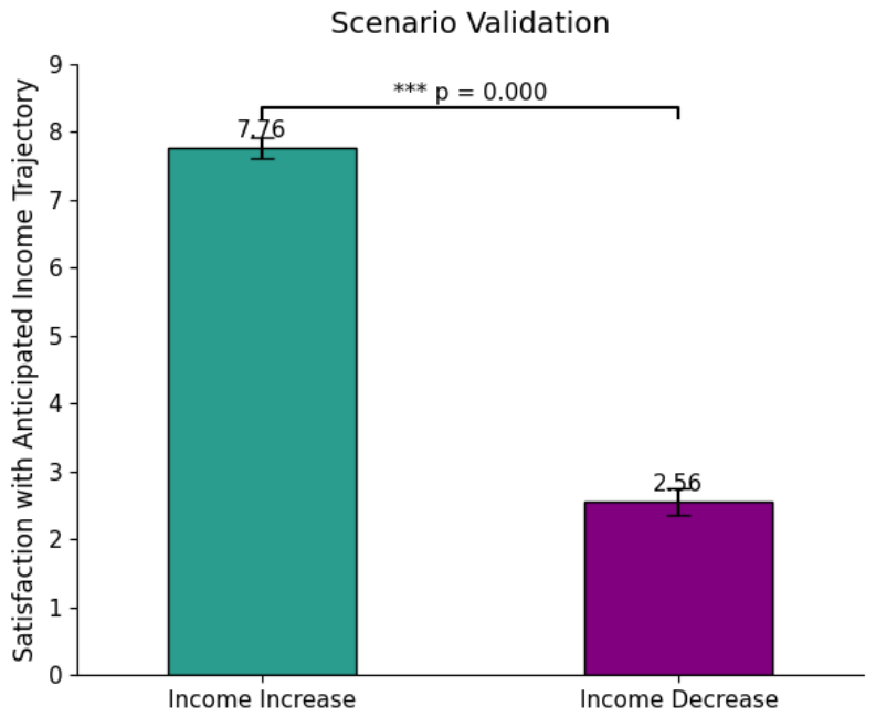
Figure A2.
Comparison of cheap product choices under income decline: Functional products vs. symbolic products.
Figure A2.
Comparison of cheap product choices under income decline: Functional products vs. symbolic products.
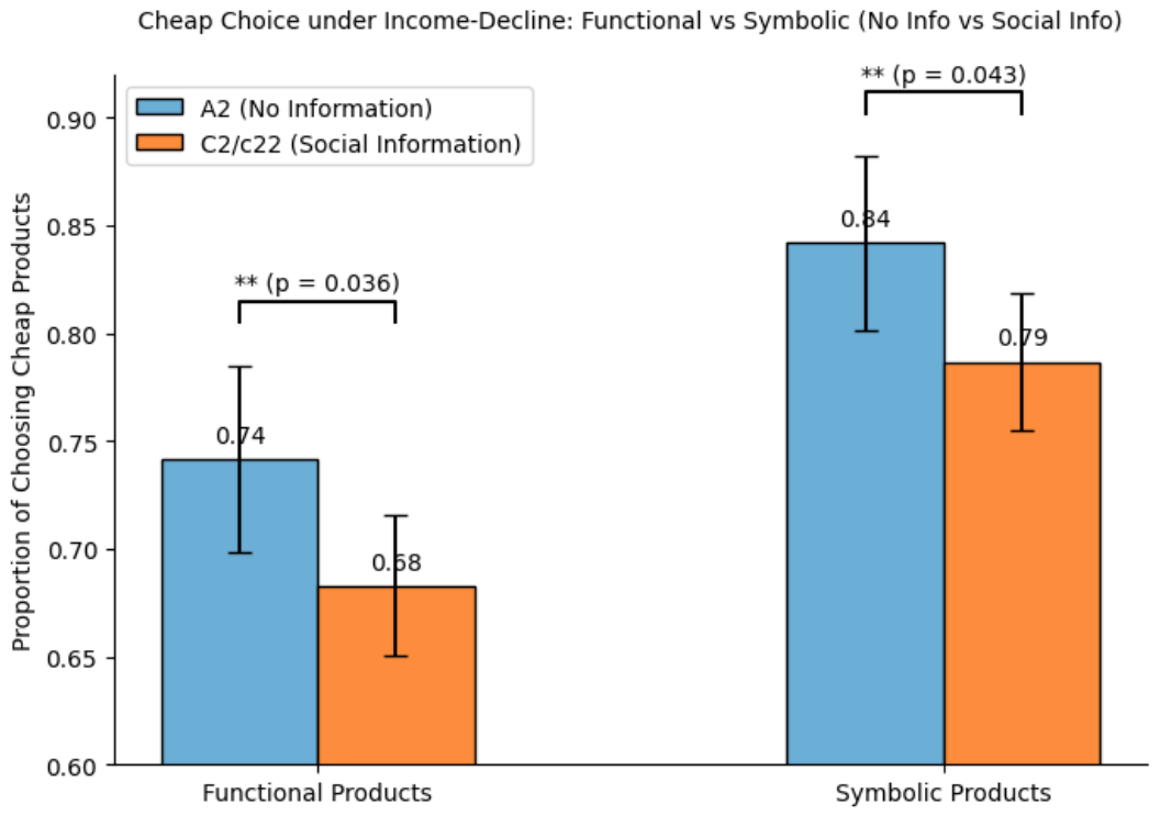
Figure A3.
Mean number of cheap product choices by income trajectory (no-information conditions: Treatment A1 vs. Treatment A2; social information conditions: the combined Treatment C1/c11 vs. the combined Treatment C2/c22). Results are based on independent-samples t-tests using participant-level totals. The error bars represent 95% confidence intervals.
Figure A3.
Mean number of cheap product choices by income trajectory (no-information conditions: Treatment A1 vs. Treatment A2; social information conditions: the combined Treatment C1/c11 vs. the combined Treatment C2/c22). Results are based on independent-samples t-tests using participant-level totals. The error bars represent 95% confidence intervals.
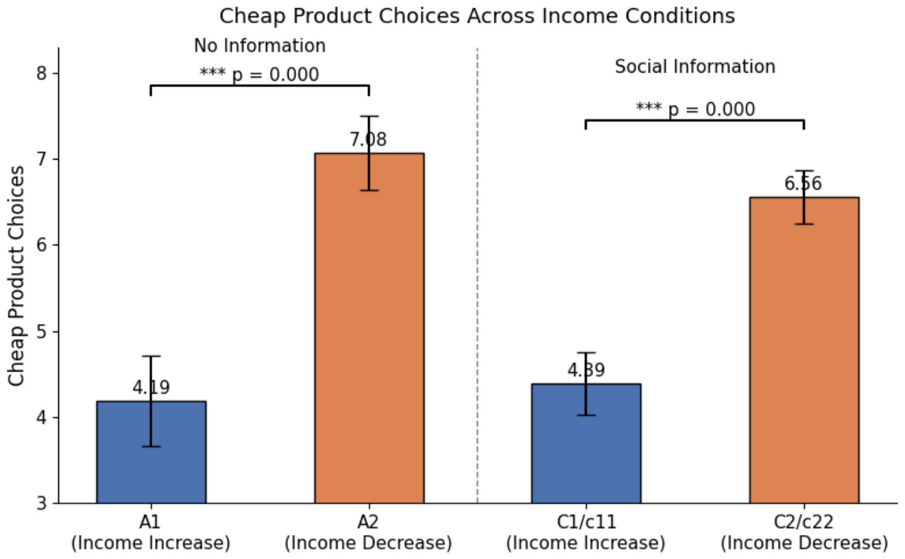
Figure A4.
Mean number of cheap product choices under income decline: no-information baseline (Treatment A2) vs. cheap-majority information condition (the combined Treatment C2/c22) within the analytical sample. Results are based on an independent-samples t-test using participant-level totals. The error bars represent 95% confidence intervals.
Figure A4.
Mean number of cheap product choices under income decline: no-information baseline (Treatment A2) vs. cheap-majority information condition (the combined Treatment C2/c22) within the analytical sample. Results are based on an independent-samples t-test using participant-level totals. The error bars represent 95% confidence intervals.
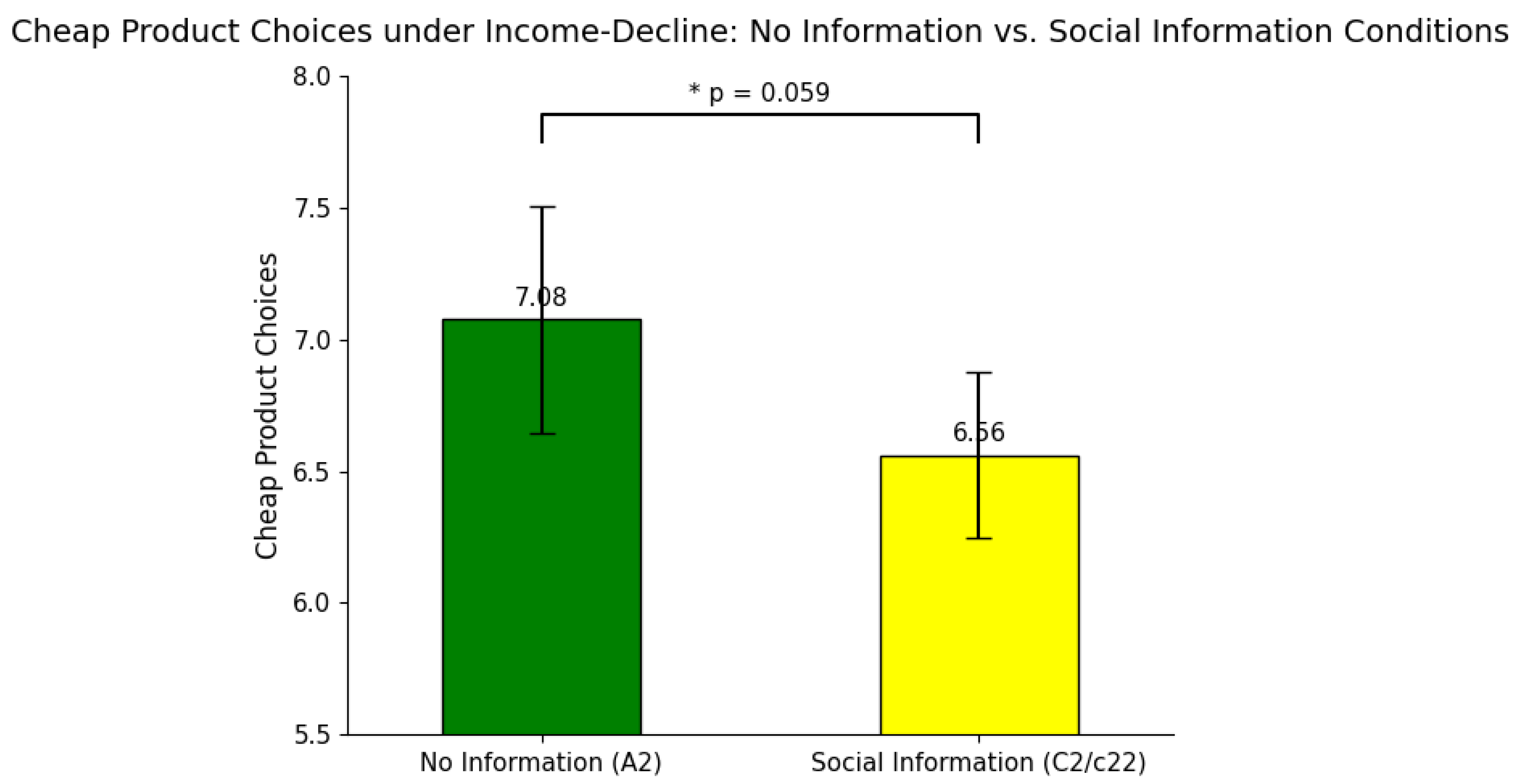
Figure A5.
Mean number of cheap product choices under income decline: no-information baseline (Treatment A2) vs. cheap-salience condition (Treatment C2) within the analytical sample. Results are based on an independent-samples t-test using participant-level totals. The error bars represent 95% confidence intervals.
Figure A5.
Mean number of cheap product choices under income decline: no-information baseline (Treatment A2) vs. cheap-salience condition (Treatment C2) within the analytical sample. Results are based on an independent-samples t-test using participant-level totals. The error bars represent 95% confidence intervals.
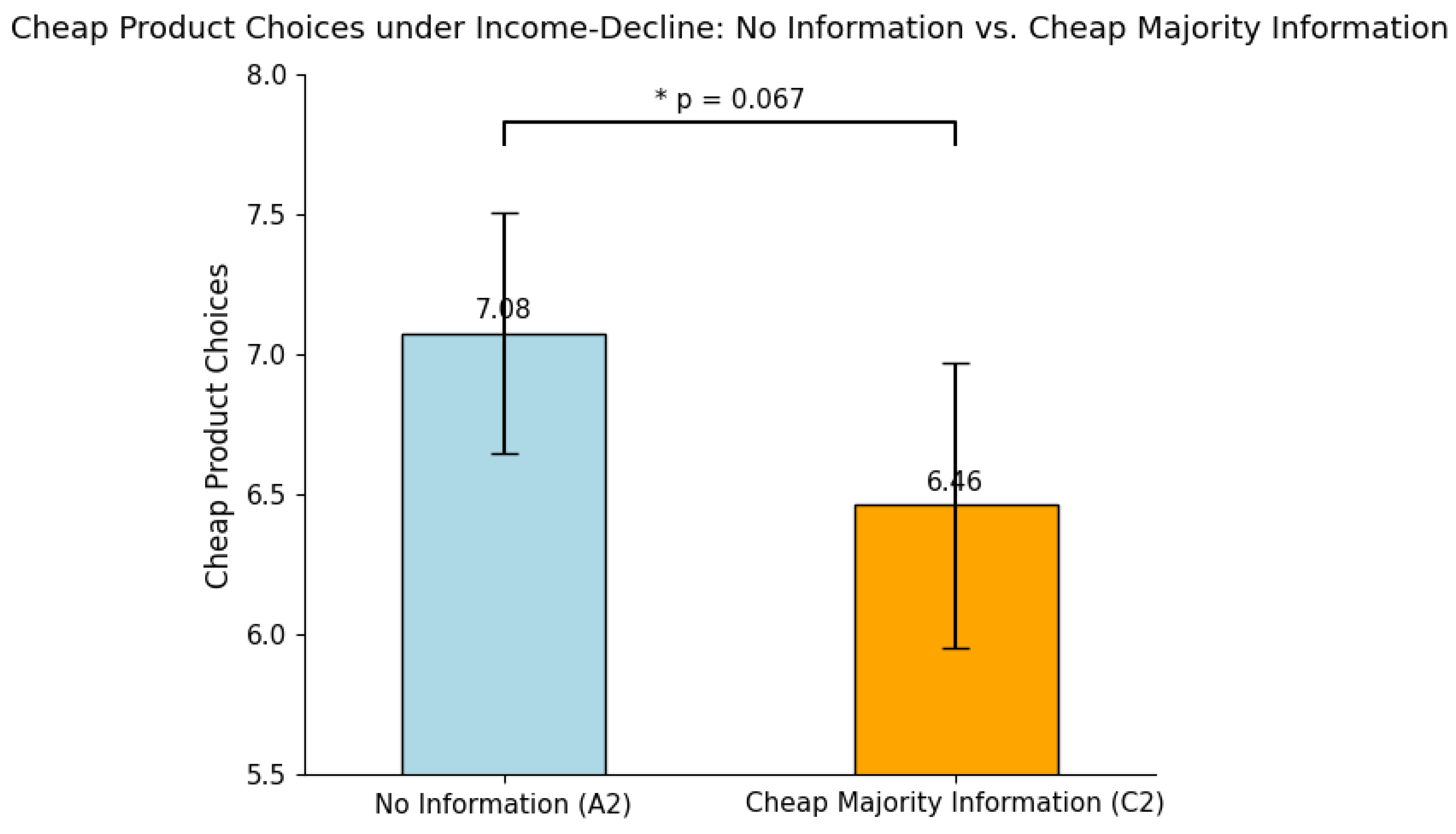
Figure A6.
Mean number of cheap product choices under income increase: cheap-majority information (Treatment C1) vs. expensive-minority information (Treatment c11), restricted to Q3, Q4, Q8, and Q12. Results are based on an independent-samples t-test using participant-level totals. Given the directional nature of Hypothesis 4A, a one-tailed p-value is reported; the corresponding two-tailed p-value is also provided. The error bars represent 95% confidence intervals.
Figure A6.
Mean number of cheap product choices under income increase: cheap-majority information (Treatment C1) vs. expensive-minority information (Treatment c11), restricted to Q3, Q4, Q8, and Q12. Results are based on an independent-samples t-test using participant-level totals. Given the directional nature of Hypothesis 4A, a one-tailed p-value is reported; the corresponding two-tailed p-value is also provided. The error bars represent 95% confidence intervals.
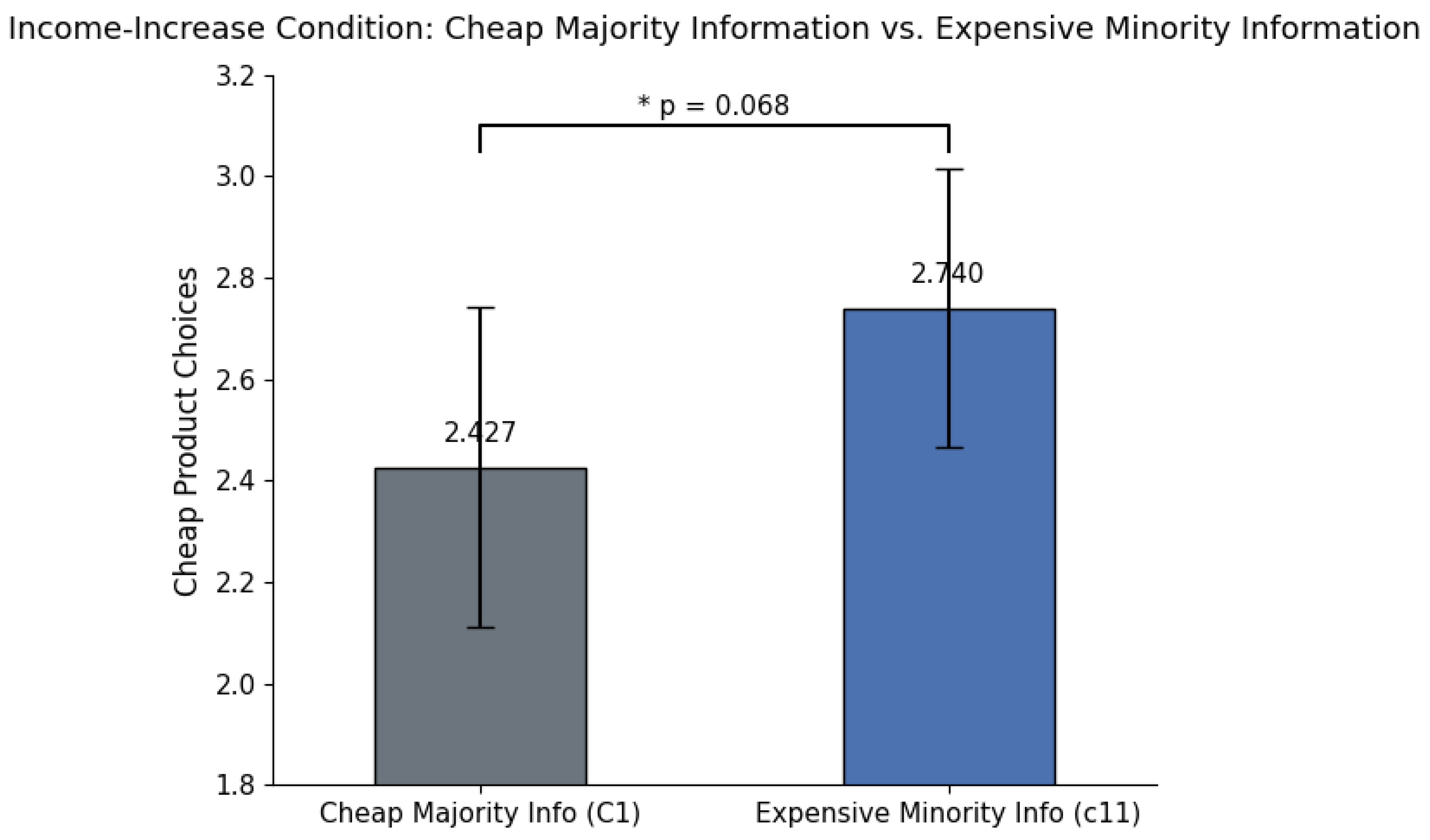
Appendix B. Questionnaire
This Appendix presents the structure of the questionnaire. The text provided is the actual English translation of the original Chinese questionnaire. While all groups followed the same overall structure, identical sections are presented only once to avoid redundancy across the six groups. The specific experimental interventions for each group, including income scenarios and social information treatments are clearly labeled and contrasted in the following sections.
Table A7.
Overview of Experimental Treatment Groups
| Group ID | Income Scenario | Social Information Treatment |
|---|---|---|
| Treatment A1 | Income Increase | No social information |
| Treatment A2 | Income Decrease | No social information |
| Treatment C1 | Income Increase | Cheap-Salience Information |
| Treatment C2 | Income Decrease | Cheap-Salience Information |
| Treatment c11 | Income Increase | Expensive-Salience Information |
| Treatment c22 | Income Decrease | Expensive-Salience Information |
Module 1: Introduction and Informed Consent (Common to All Groups)
Thank you for participating in this academic study. Before proceeding, please read the following information carefully.
-
Study ContentThis study focuses on consumption behavior. You will be asked to make choices among different consumer products.
-
DurationApproximately 5 minutes.
-
Data ConfidentialityAll responses will be used for academic research purposes only and will be kept strictly confidential.
-
CompensationYou will receive RMB 1 upon completing the questionnaire, provided that your responses meet the validity requirements described below.
-
Response RequirementsPlease read each question carefully and answer truthfully. The questionnaire contains two attention-check questions. If these are answered incorrectly, the questionnaire will be considered invalid.
-
Informed ConsentBy completing and submitting this questionnaire, you acknowledge that you understand the above information and voluntarily agree to participate. You may exit the survey at any time if you do not wish to continue.
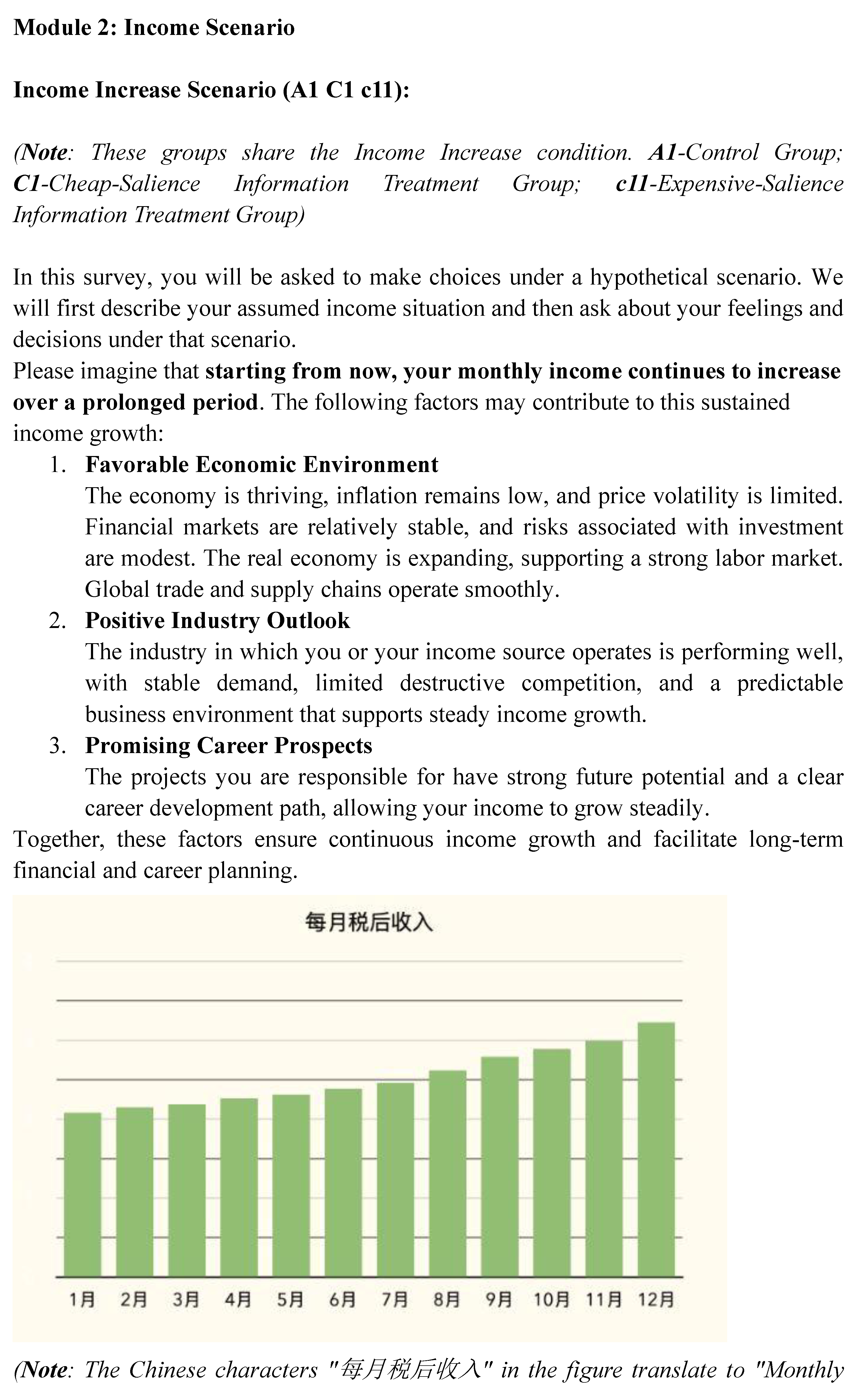
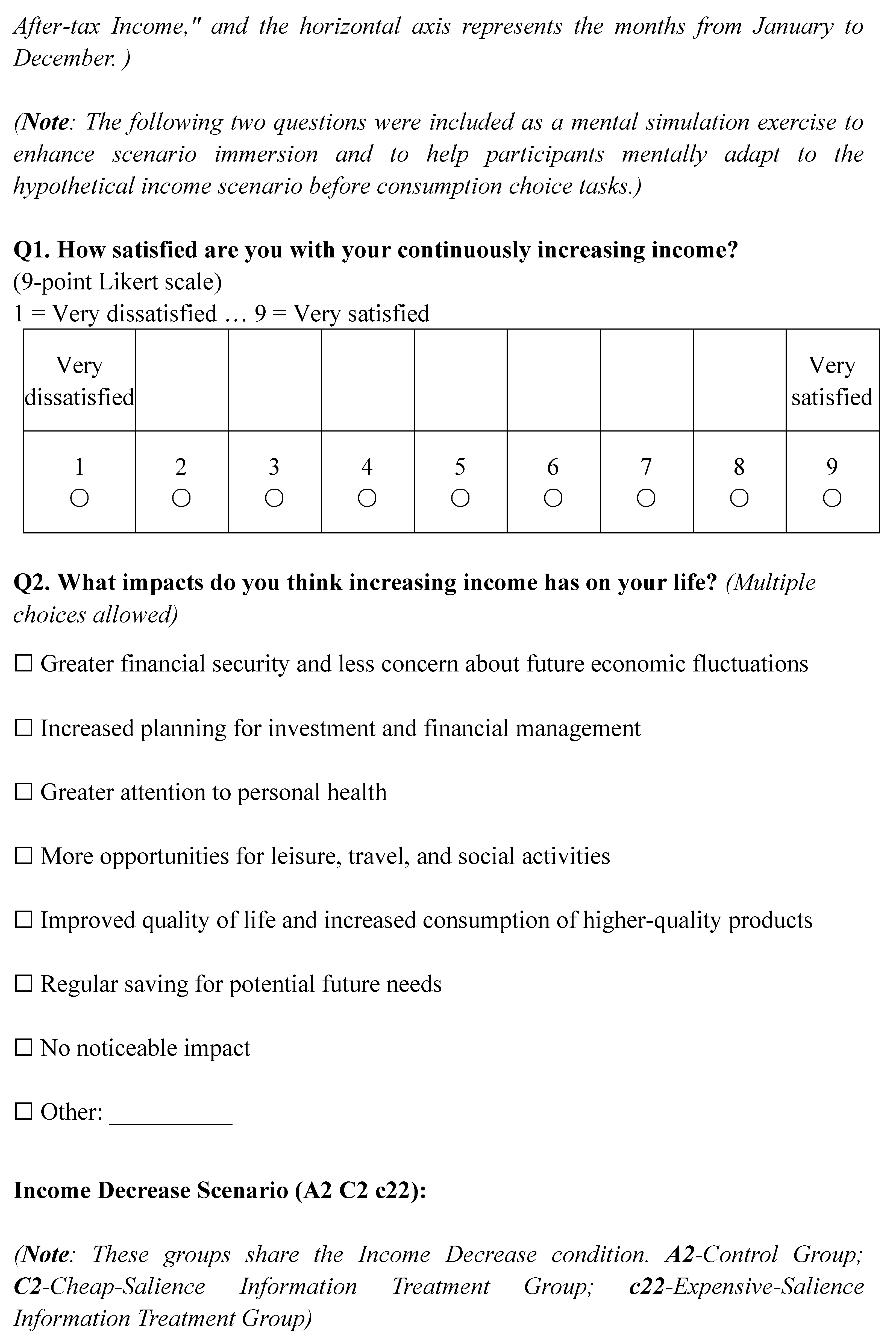
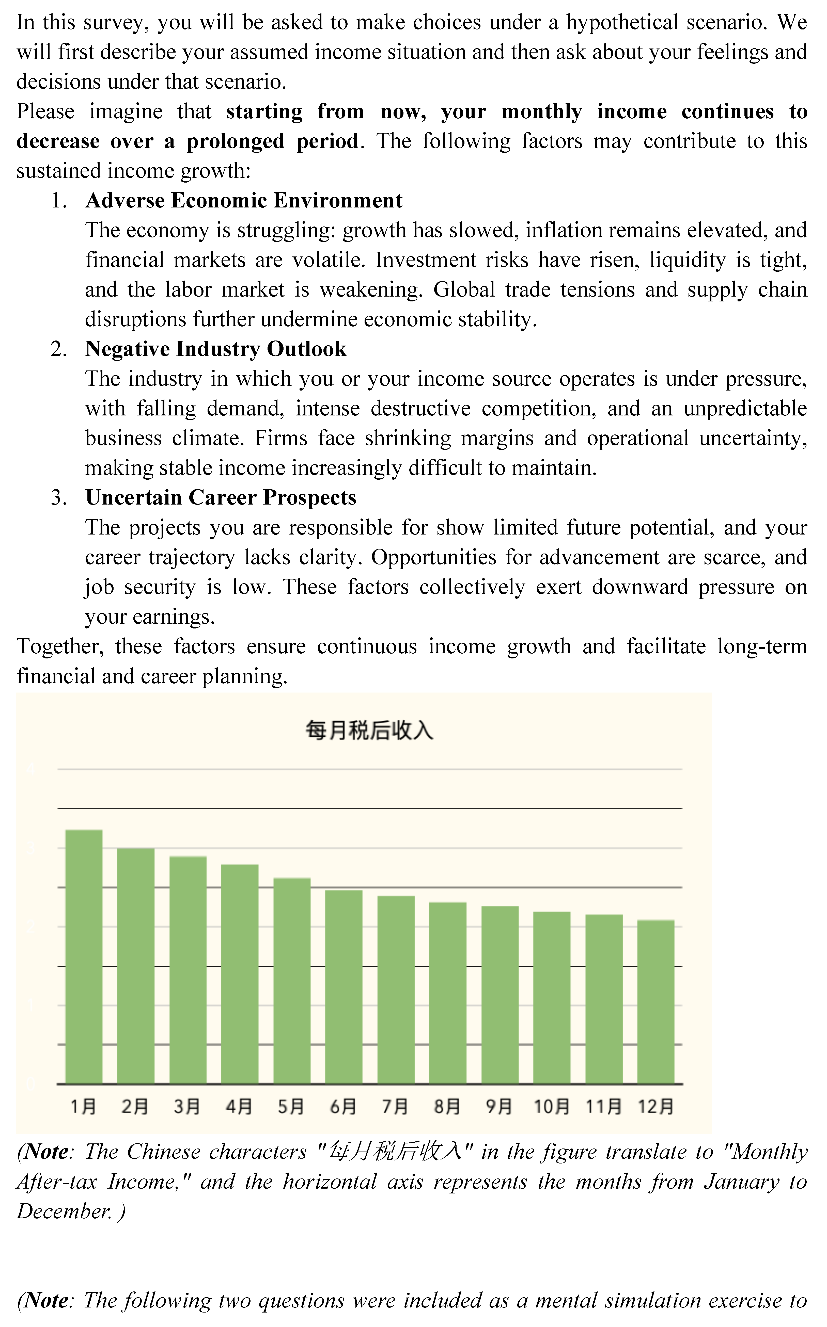

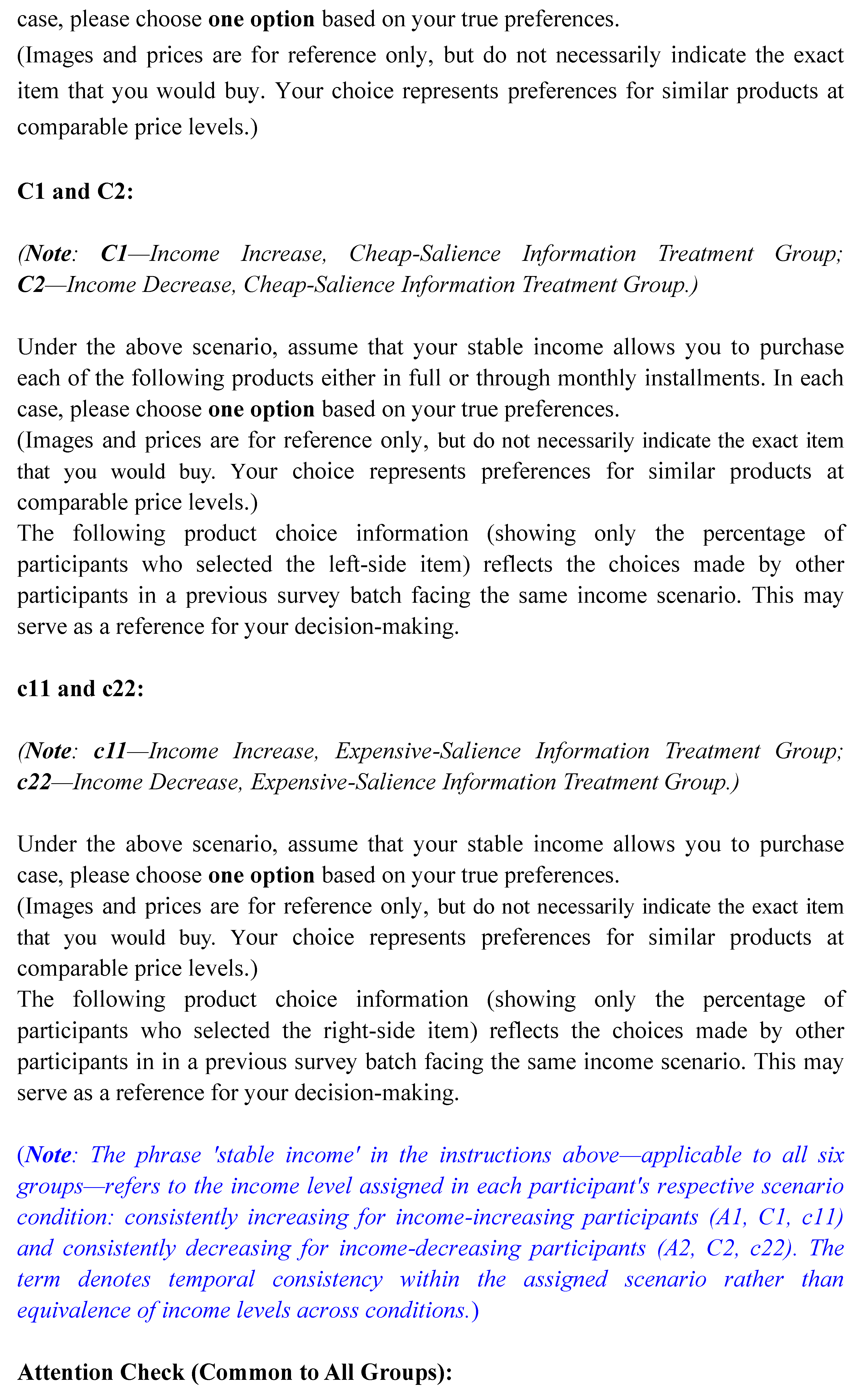
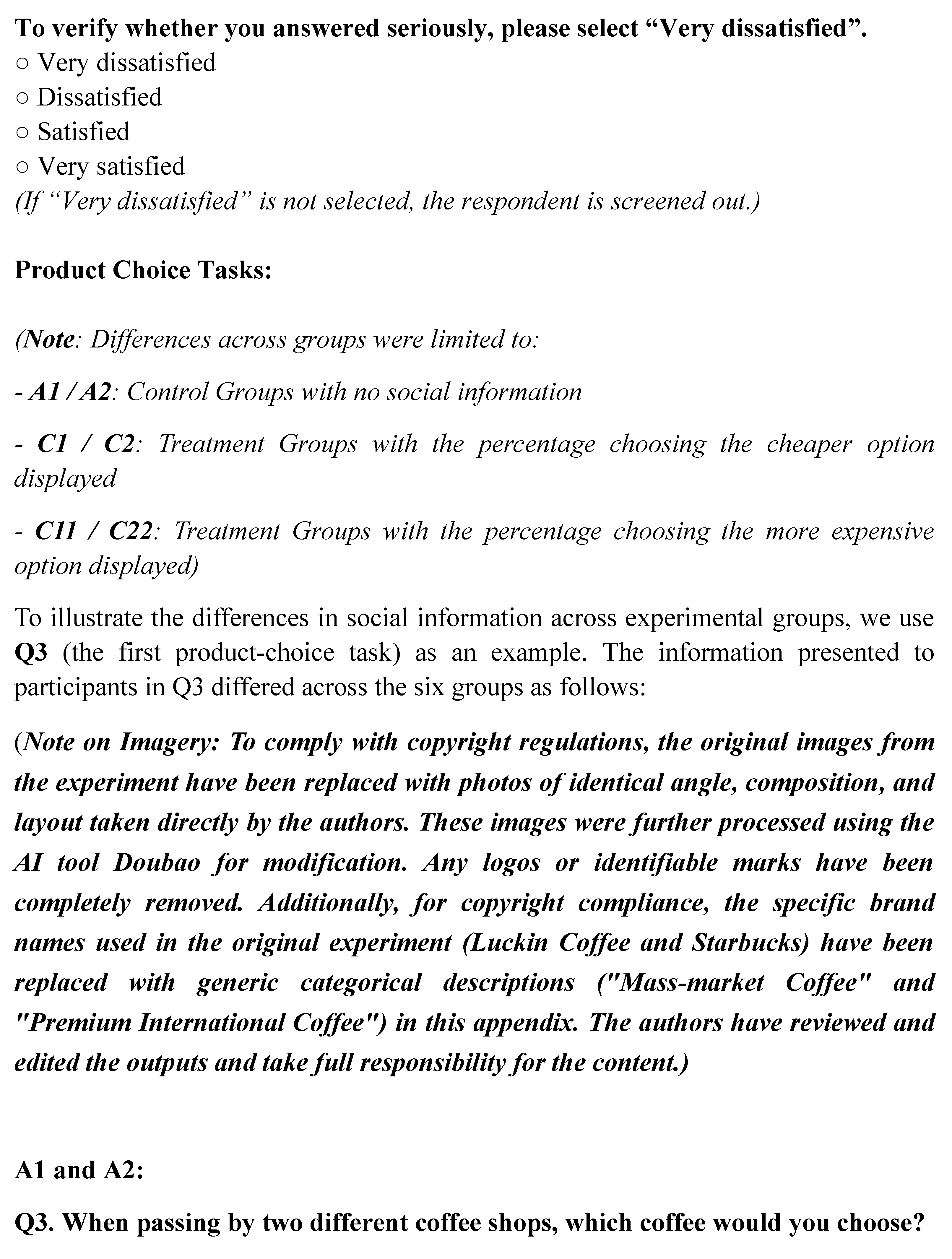
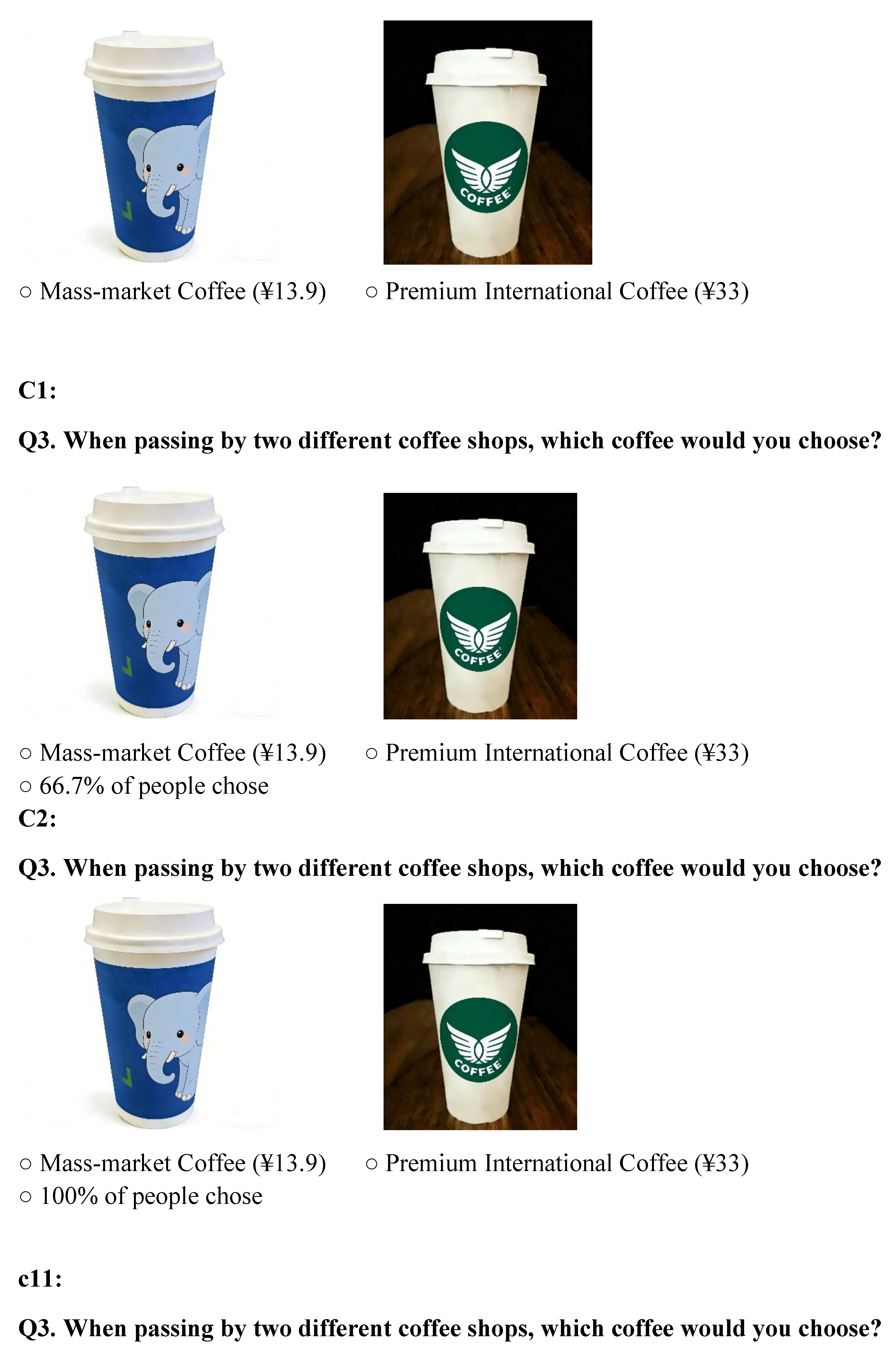
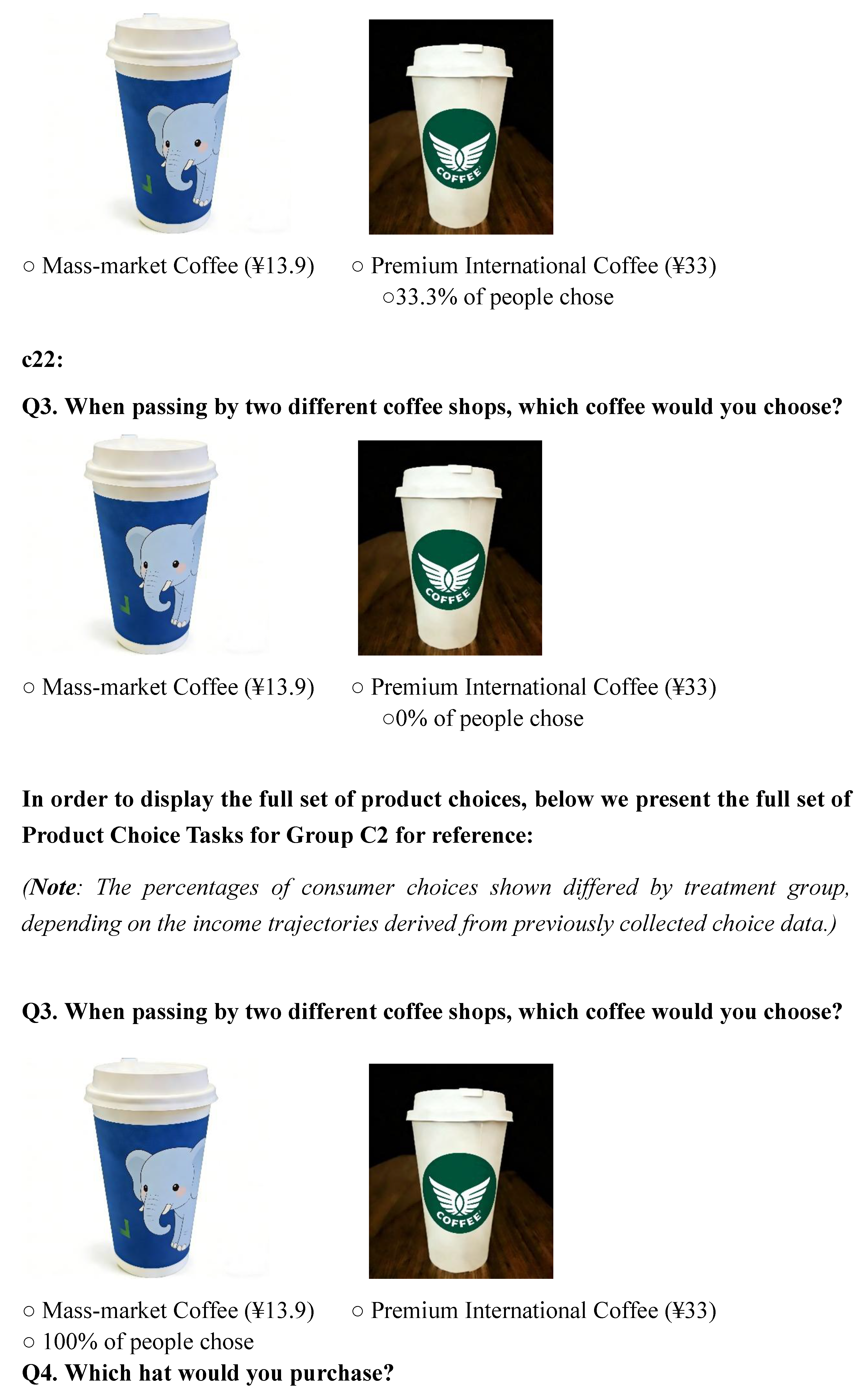
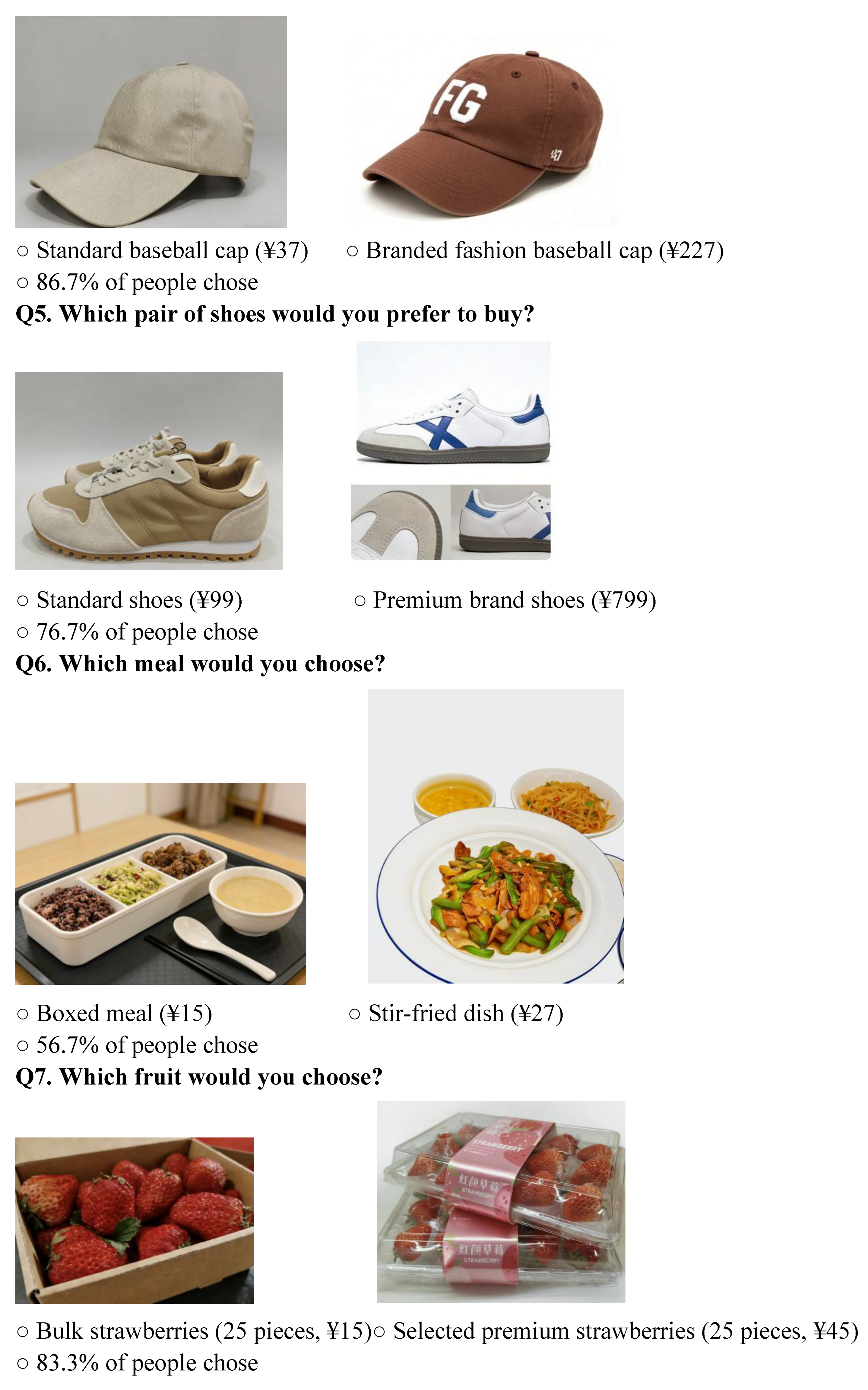
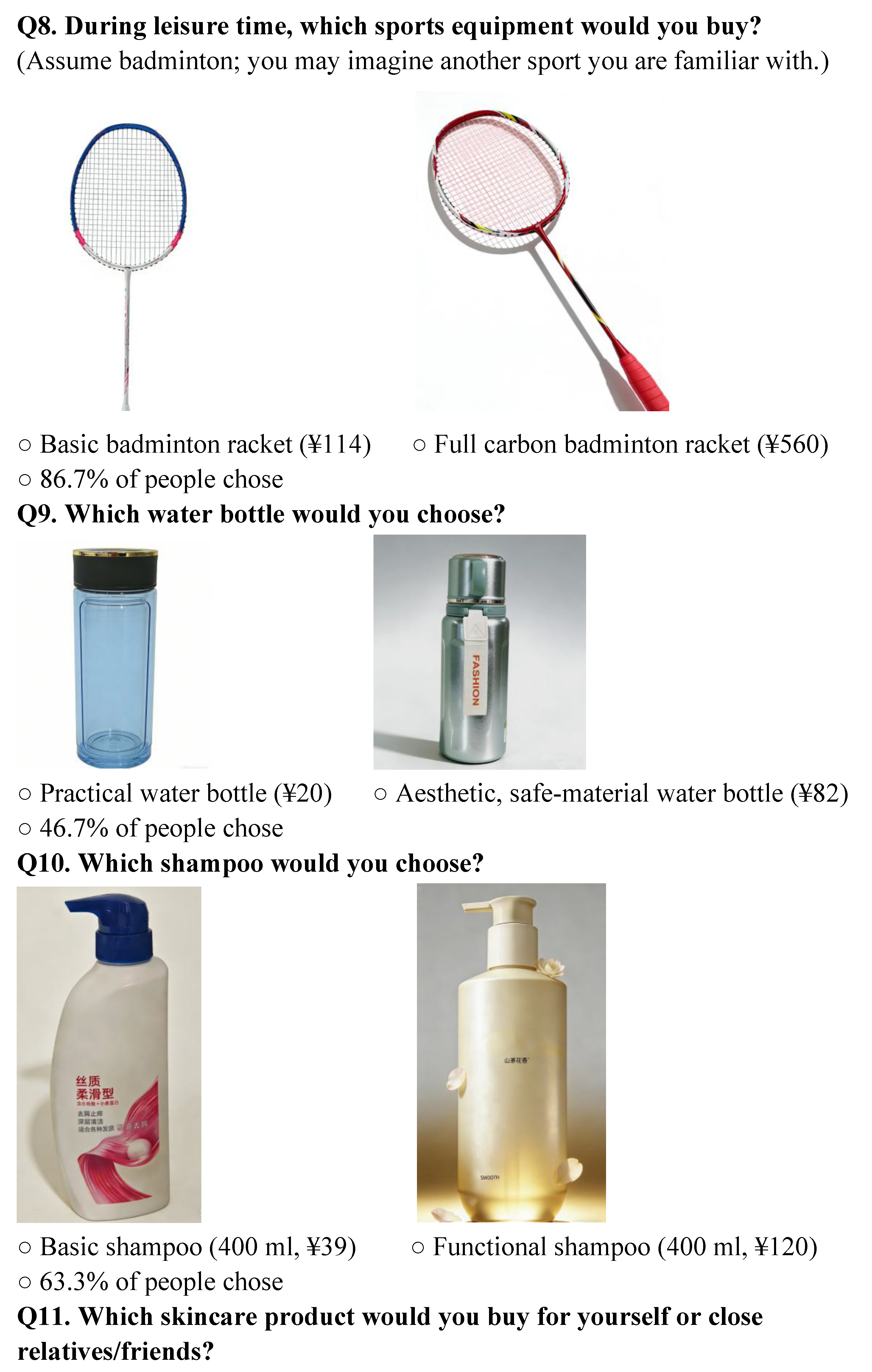
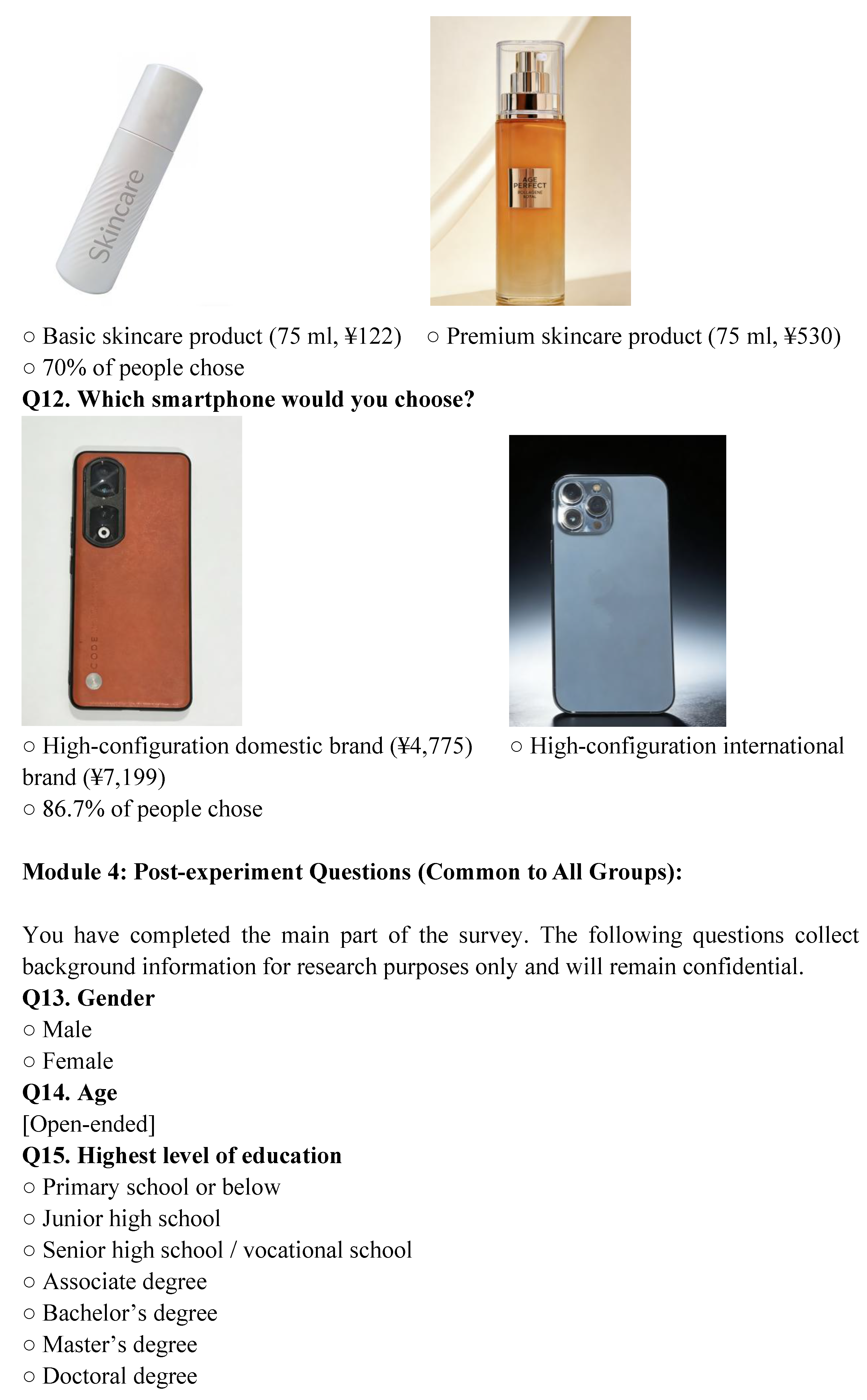
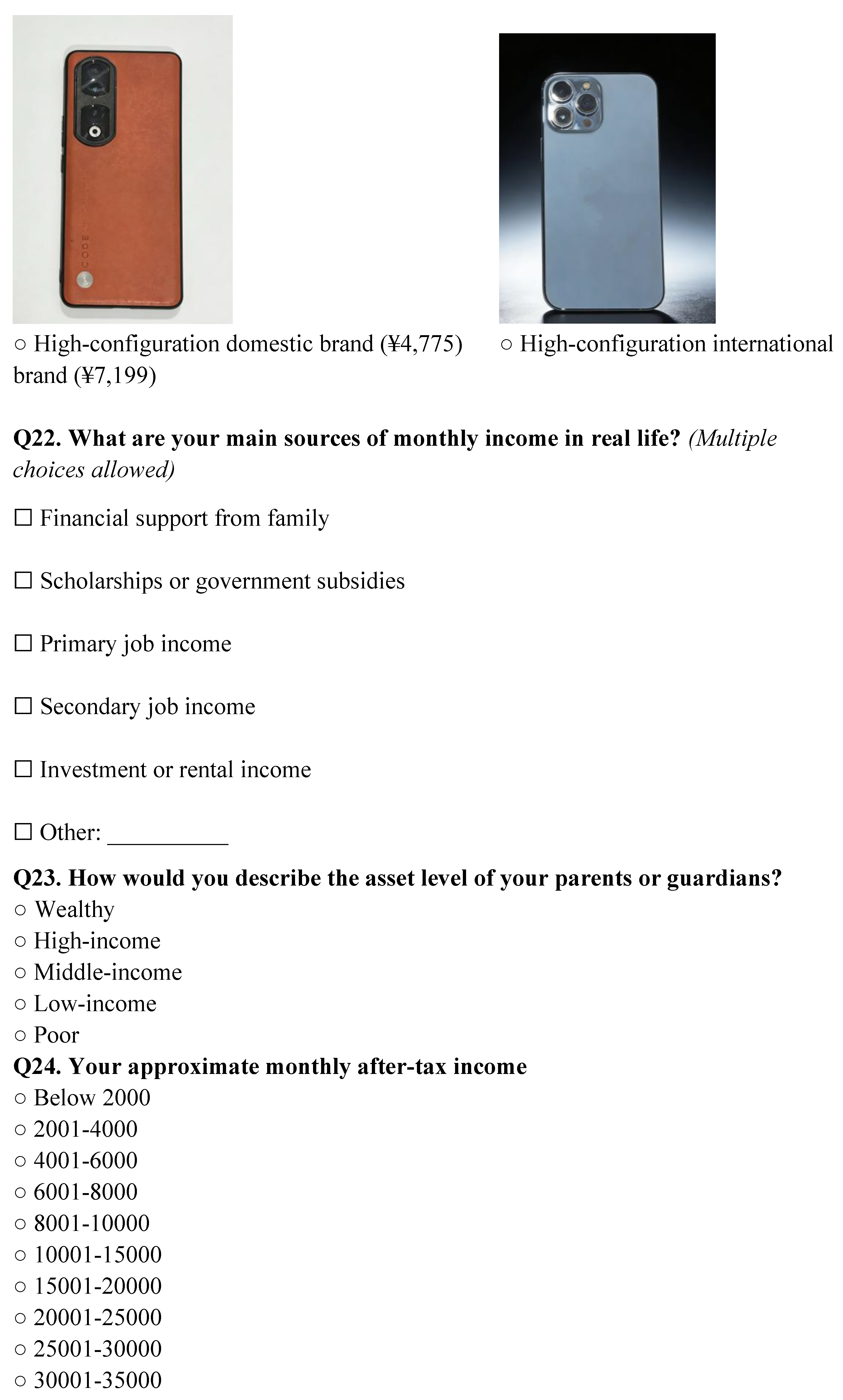
References
- Friedman, M. Front Matter“ A Theory of the Consumption Function”. In A theory of the consumption function; Princeton University Press, 1957; pp. 20–0.
- Banerjee, A.V. A simple model of herd behavior. The quarterly journal of economics 1992, 107, 797–817. [CrossRef]
- Guvenen, F.; Karahan, F.; Ozkan, S.; Song, J. What do data on millions of US workers reveal about lifecycle earnings dynamics? Econometrica 2021, 89, 2303–2339. [CrossRef]
- Coibion, O.; Gorodnichenko, Y.; Weber, M. Monetary policy communications and their effects on household inflation expectations. Journal of Political Economy 2022, 130, 1537–1584. [CrossRef]
- DellaVigna, S. Psychology and economics: Evidence from the field. Journal of Economic literature 2009, 47, 315–372. [CrossRef]
- Chetty, R.; Looney, A.; Kroft, K. Salience and taxation: Theory and evidence. American economic review 2009, 99, 1145–1177. [CrossRef]
- Chopra, F.; Roth, C.; Wohlfart, J. Home price expectations and spending: Evidence from a field experiment. American Economic Review 2025, 115, 2267–2305. [CrossRef]
- Beshears, J.; Choi, J.J.; Laibson, D.; Madrian, B.C. How are preferences revealed? Journal of public economics 2008, 92, 1787–1794. [CrossRef]
- Bursztyn, L.; González, A.L.; Yanagizawa-Drott, D. Misperceived social norms: Women working outside the home in Saudi Arabia. American economic review 2020, 110, 2997–3029. [CrossRef]
- Grossman, G.M.; Helpman, E. Identity politics and trade policy. The Review of Economic Studies 2021, 88, 1101–1126.
- Lien, J.W.; Zheng, J. Deciding when to quit: Reference-dependence over slot machine outcomes. American Economic Review 2015, 105, 366–370. [CrossRef]
- Ganong, P.; Noel, P.; Vavra, J. US unemployment insurance replacement rates during the pandemic. Journal of public economics 2020, 191, 104273. [CrossRef]
- Baker, S.R.; Farrokhnia, R.A.; Meyer, S.; Pagel, M.; Yannelis, C. Income, liquidity, and the consumption response to the 2020 economic stimulus payments. Review of Finance 2023, 27, 2271–2304. [CrossRef]
- D’Acunto, F.; Hoang, D.; Weber, M. Managing households’ expectations with unconventional policies. The Review of Financial Studies 2022, 35, 1597–1642.
- LeBoeuf, R.A.; Shafir, E. The long and short of it: Physical anchoring effects. Journal of Behavioral Decision Making 2006, 19, 393–406. [CrossRef]
- Bonomi, G.; Gennaioli, N.; Tabellini, G. Identity, beliefs, and political conflict. The Quarterly Journal of Economics 2021, 136, 2371–2411. [CrossRef]
- Mazar, N.; Amir, O.; Ariely, D. The dishonesty of honest people: A theory of self-concept maintenance. Journal of marketing research 2008, 45, 633–644. [CrossRef]
- Hainmueller, J.; Hangartner, D.; Yamamoto, T. Validating vignette and conjoint survey experiments against real-world behavior. Proceedings of the National Academy of Sciences 2015, 112, 2395–2400. [CrossRef]
- Aguinis, H.; Bradley, K.J. Best practice recommendations for designing and implementing experimental vignette methodology studies. Organizational research methods 2014, 17, 351–371. [CrossRef]
- Krupka, E.L.; Weber, R.A. Identifying social norms using coordination games: Why does dictator game sharing vary? Journal of the European Economic Association 2013, 11, 495–524. [CrossRef]
- Bursztyn, L.; Jensen, R. Social image and economic behavior in the field: Identifying, understanding, and shaping social pressure. Annual Review of Economics 2017, 9, 131–153. [CrossRef]
- White, K.; Dahl, D.W. To be or not be? The influence of dissociative reference groups on consumer preferences. Journal of Consumer Psychology 2006, 16, 404–414. [CrossRef]
- Bertrand, M.; Morse, A. Trickle-down consumption. Review of Economics and Statistics 2016, 98, 863–879. [CrossRef]
- Willis, G.B.; García-Sánchez, E.; Sánchez-Rodríguez, Á.; García-Castro, J.D.; Rodríguez-Bailón, R. The psychosocial effects of economic inequality depend on its perception. Nature Reviews Psychology 2022, 1, 301–309. [CrossRef]
- Meier, S.; Sprenger, C. Present-biased preferences and credit card borrowing. American Economic Journal: Applied Economics 2010, 2, 193–210. [CrossRef]
- Kraus, M.W.; Park, J.W.; Tan, J.J. Signs of social class: The experience of economic inequality in everyday life. Perspectives on Psychological Science 2017, 12, 422–435. [CrossRef]
- Allison, P.D. Comparing logit and probit coefficients across groups. Sociological methods & research 1999, 28, 186–208. [CrossRef]
- de Palma, A.; Picard, N. Route choice decision under travel time uncertainty. Transportation Research Part A: Policy and Practice 2005, 39, 295–324. [CrossRef]
- Griskevicius, V.; Tybur, J.M.; Van den Bergh, B. Going green to be seen: Status, reputation, and conspicuous conservation. Journal of personality and social psychology 2010, 98, 392. [CrossRef]
- Bertrand, M.; Kamenica, E.; Pan, J. Gender identity and relative income within households. The Quarterly Journal of Economics 2015, 130, 571–614. [CrossRef]
- Bursztyn, L.; Egorov, G.; Fiorin, S. From extreme to mainstream: The erosion of social norms. American economic review 2020, 110, 3522–3548. [CrossRef]
- Berger, J.; Heath, C. Where consumers diverge from others: Identity signaling and product domains. Journal of consumer research 2007, 34, 121–134. [CrossRef]
- Weber, E.U.; Blais, A.R.; Betz, N.E. A domain-specific risk-attitude scale: Measuring risk perceptions and risk behaviors. Journal of behavioral decision making 2002, 15, 263–290. [CrossRef]
- Beck, M.J.; Fifer, S.; Rose, J.M. Can you ever be certain? Reducing hypothetical bias in stated choice experiments via respondent reported choice certainty. Transportation Research Part B: Methodological 2016, 89, 149–167. [CrossRef]
- De Chaisemartin, C.; d’Haultfoeuille, X. Two-way fixed effects estimators with heterogeneous treatment effects. American economic review 2020, 110, 2964–2996. [CrossRef]
| 1 | We identified nine participant IDs that appeared across multiple experimental conditions due to platform assignment anomalies. For these participants, only the first completed response was retained, yielding a final valid analytic sample of 468 participants (Treatment A1: 80, Treatment A2: 79, Treatment C1: 75, Treatment C2: 78, Treatment c11: 77, Treatment c22: 79). All results reported in this paper are based on this sample. |
| 2 | The pilot questionnaire and use of the choice data from the pilot as the source of information in the main task derives from the practice in experimental economics that subjects shall not be deceived at any point in the experiment. Thus, any information provided to subjects in the study should reflect a reality, and we follow this practice in this experiment. |
Figure 1.
Treatment Group Chart. Note: Information in these treatments is based on actual choices in the pilot survey (Group A, N = 30). Capital letters (C) show the percentage choosing the cheaper product (e.g., 60% in A2), while lowercase letters (c) show the remaining percentage choosing the premium product (e.g., 40%).
Figure 1.
Treatment Group Chart. Note: Information in these treatments is based on actual choices in the pilot survey (Group A, N = 30). Capital letters (C) show the percentage choosing the cheaper product (e.g., 60% in A2), while lowercase letters (c) show the remaining percentage choosing the premium product (e.g., 40%).
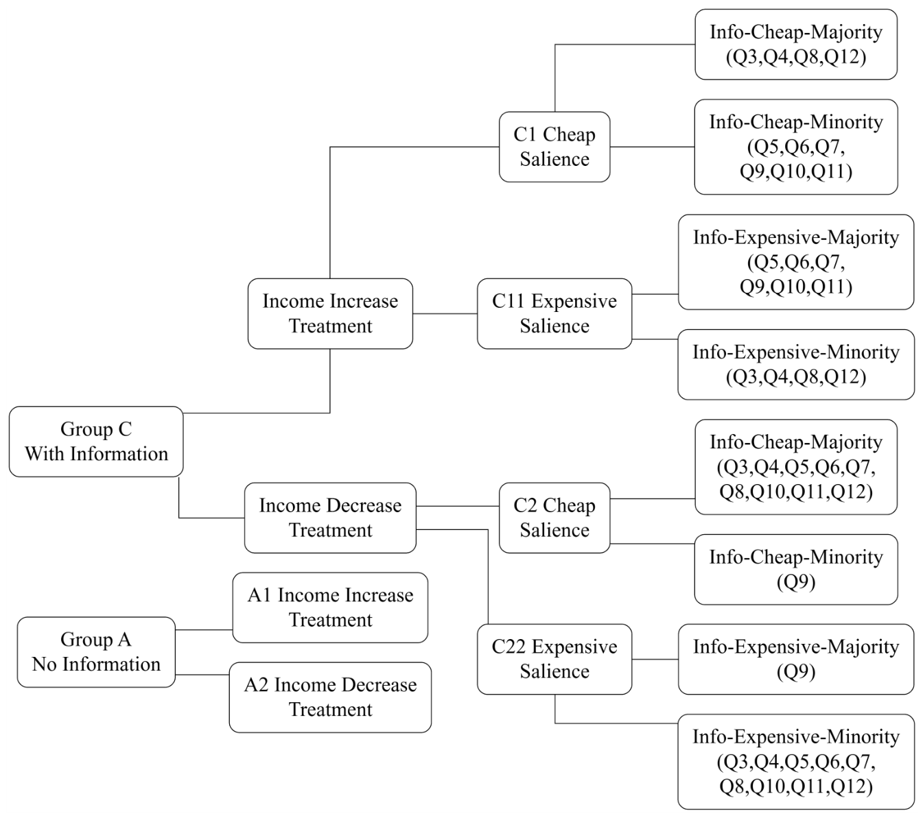
Figure 2.
Examples of Choices with Information. Panel A (left) illustrates the cheap salience treatment; Panel B (right) illustrates the expensive salience treatment. Both panels present complementary information derived from the same underlying choice data.
Figure 2.
Examples of Choices with Information. Panel A (left) illustrates the cheap salience treatment; Panel B (right) illustrates the expensive salience treatment. Both panels present complementary information derived from the same underlying choice data.
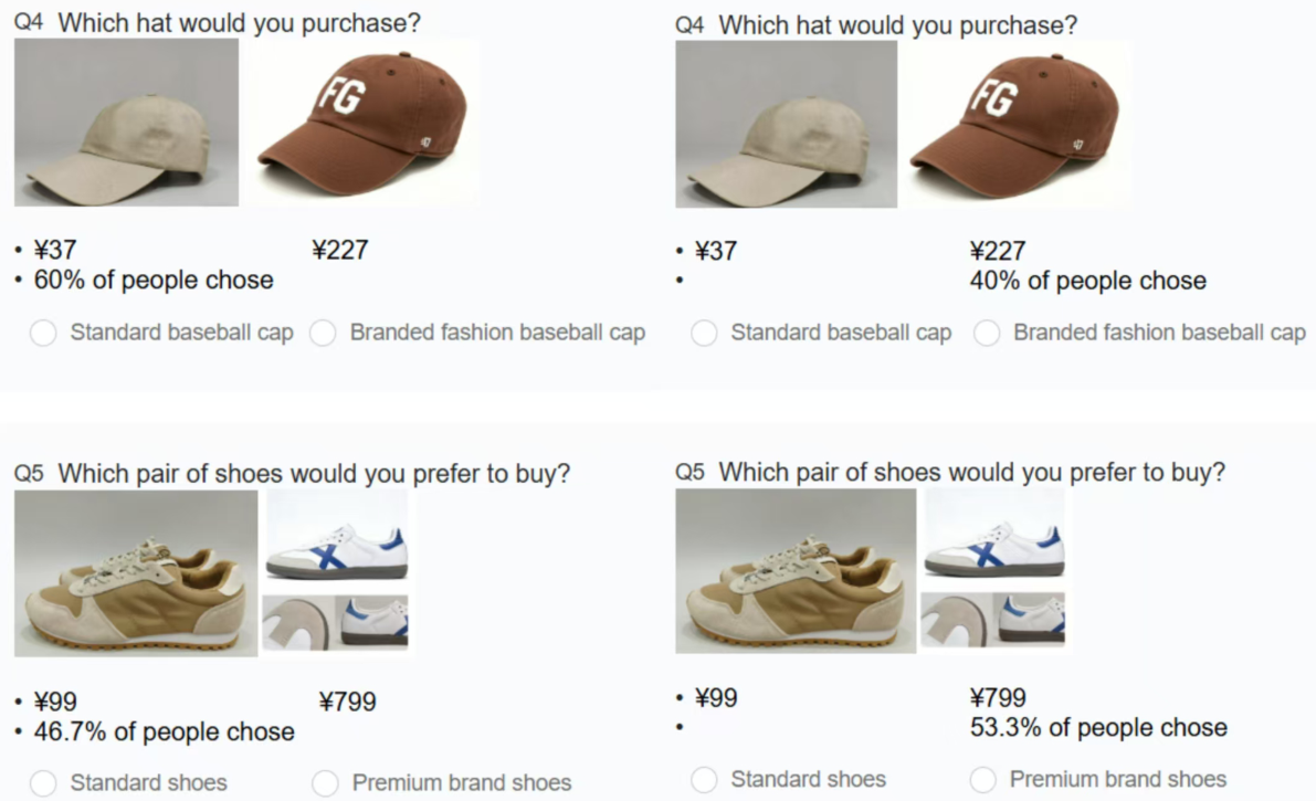
Figure 3.
Proportion of cheap product choices by income trajectory. Left panel: no-information conditions (Treatment A1 vs. Treatment A2). Right panel: social information conditions (the combined Treatment C1/c11 vs. the combined Treatment C2/c22). The error bars represent 95% confidence intervals.
Figure 3.
Proportion of cheap product choices by income trajectory. Left panel: no-information conditions (Treatment A1 vs. Treatment A2). Right panel: social information conditions (the combined Treatment C1/c11 vs. the combined Treatment C2/c22). The error bars represent 95% confidence intervals.
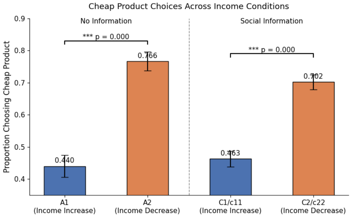
Figure 4.
Proportion of cheap product choices under income decline: no-information baseline (Treatment A2) vs. cheap-majority information combined with expensive-minority information condition (the combined Treatment C2/c22) within the analytical sample. The error bars represent 95% confidence intervals.
Figure 4.
Proportion of cheap product choices under income decline: no-information baseline (Treatment A2) vs. cheap-majority information combined with expensive-minority information condition (the combined Treatment C2/c22) within the analytical sample. The error bars represent 95% confidence intervals.
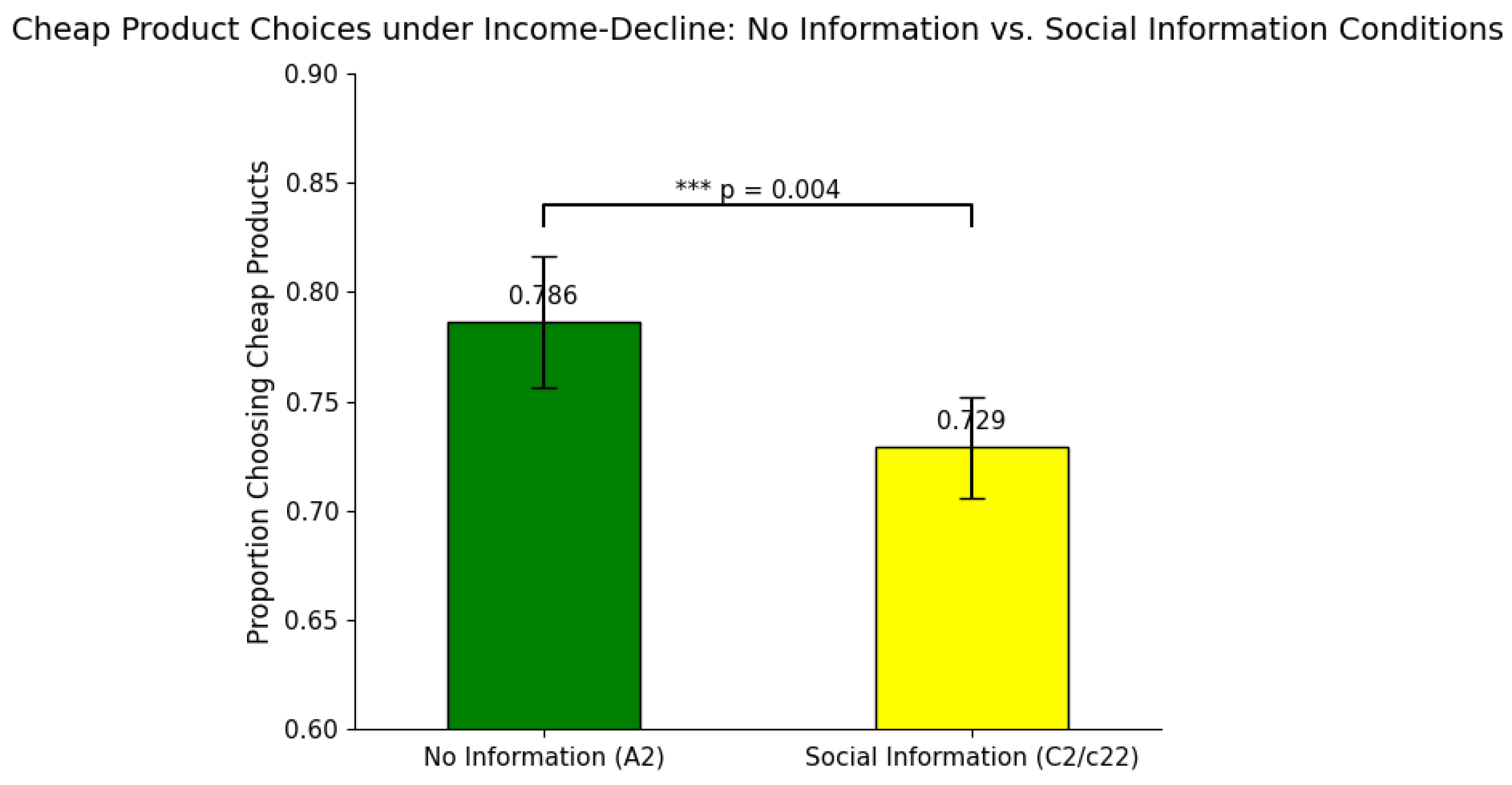
Figure 5.
Proportion of cheap product choices under income decline: no-information baseline (Treatment A2) vs. cheap-majority information condition (Treatment C2) within the analytical sample. The error bars represent 95% confidence intervals.
Figure 5.
Proportion of cheap product choices under income decline: no-information baseline (Treatment A2) vs. cheap-majority information condition (Treatment C2) within the analytical sample. The error bars represent 95% confidence intervals.
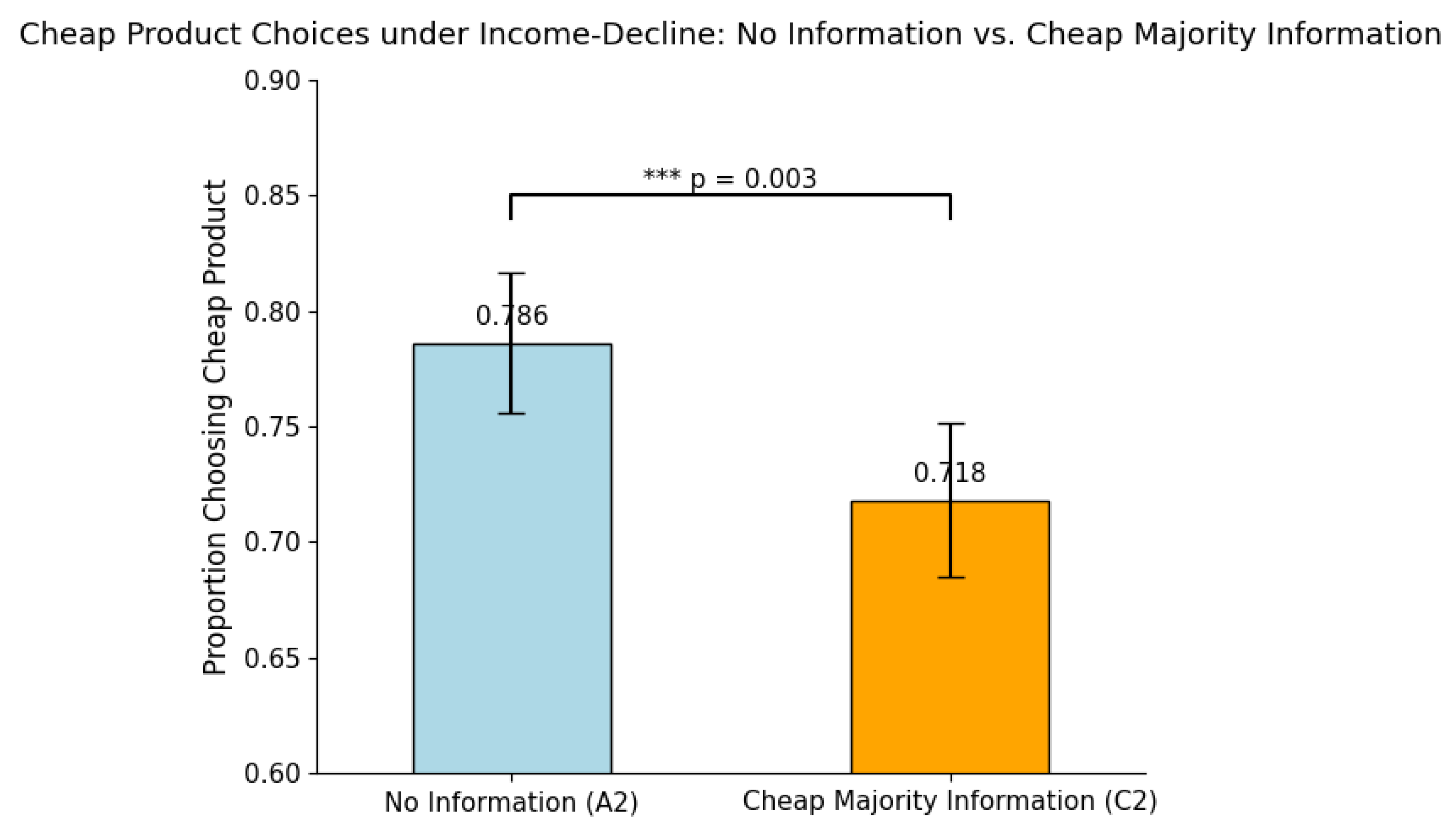
Figure 6.
Proportion of cheap product choices under income increase: cheap-majority information (Treatment C1) vs. expensive-minority information (Treatment c11), restricted to Q3, Q4, Q8, and Q12. Given the directional nature of Hypothesis 6, a one-tailed p-value is reported (); the corresponding two-tailed p-value is . The error bars represent 95% confidence intervals.
Figure 6.
Proportion of cheap product choices under income increase: cheap-majority information (Treatment C1) vs. expensive-minority information (Treatment c11), restricted to Q3, Q4, Q8, and Q12. Given the directional nature of Hypothesis 6, a one-tailed p-value is reported (); the corresponding two-tailed p-value is . The error bars represent 95% confidence intervals.
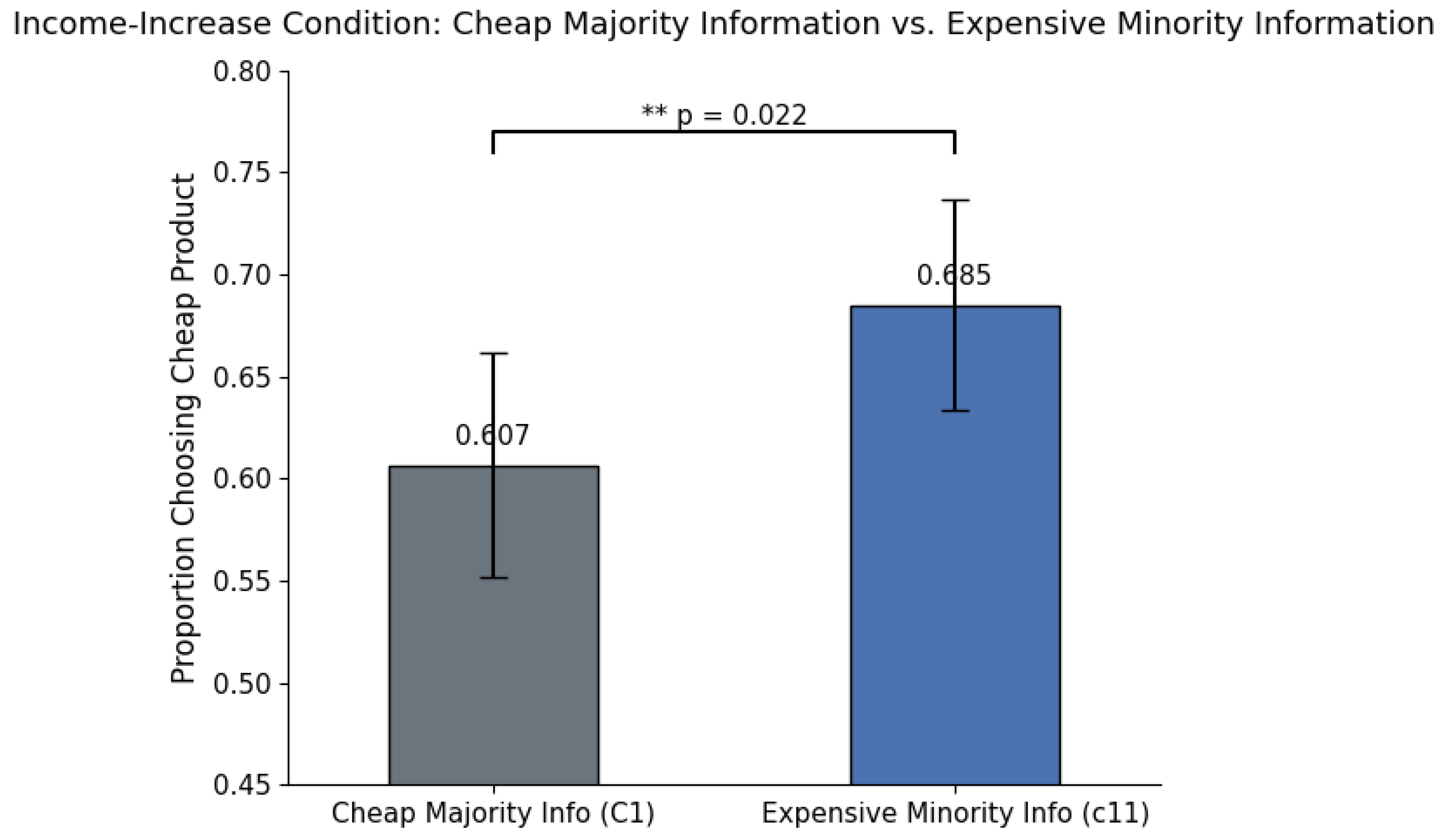
Figure 7.
Heterogeneous Effects: (a) Gender Difference; (b) Income Difference; (c) Age Difference; (d) Residence Difference.
Figure 7.
Heterogeneous Effects: (a) Gender Difference; (b) Income Difference; (c) Age Difference; (d) Residence Difference.
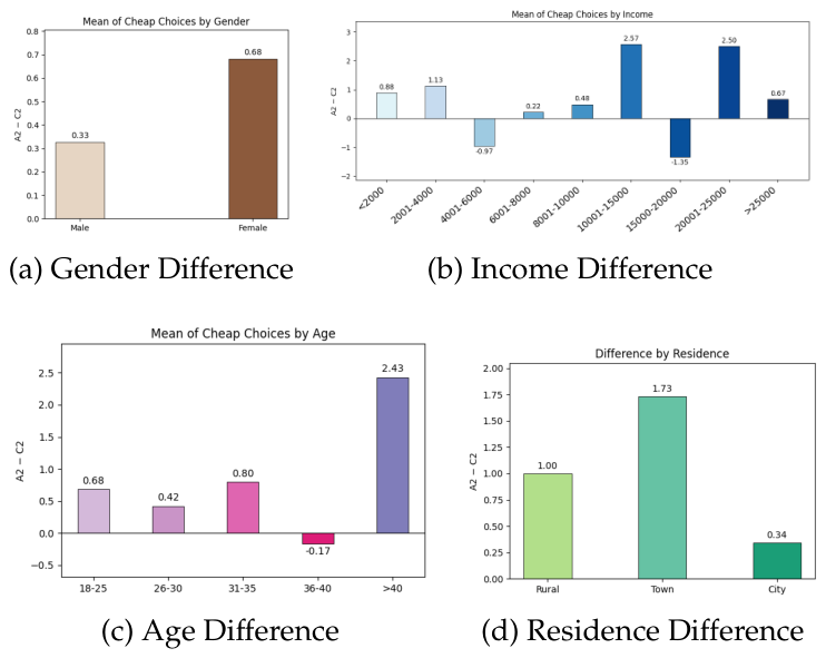
Table 2.
Summary of Cheap Product Choices Across All Experimental Conditions.
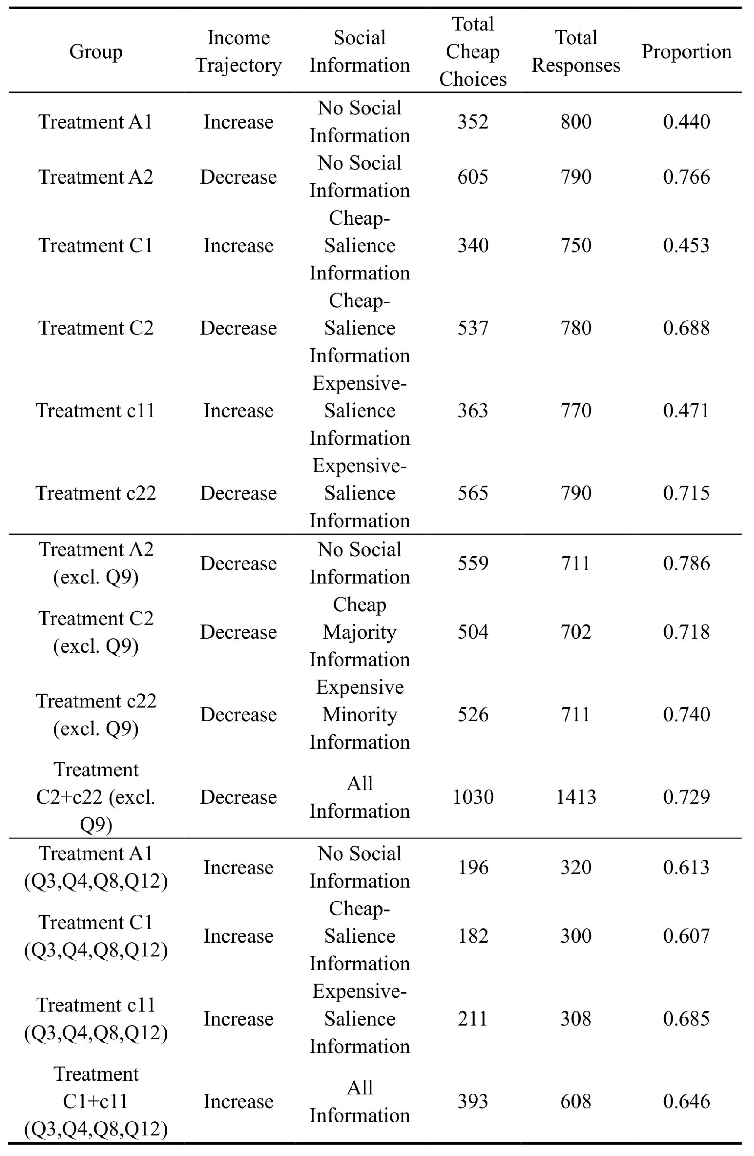 |
Notes: The final valid sample consists of 468 participants (Treatment A1: 80, Treatment A2: 79, Treatment C1: 75, Treatment C2: 78, Treatment c11: 77, Treatment c22: 79). Total responses reflect the actual number of valid responses per group. The second panel reports the analytical sample (Q9 excluded). The third panel restricts cheap product choices to Q3, Q4, Q8, and Q12, the four products for which cheap-majority information was displayed under the income-increase trajectory. Proportions are calculated as total cheap choices divided by total valid responses within each panel.
Disclaimer/Publisher’s Note: The statements, opinions and data contained in all publications are solely those of the individual author(s) and contributor(s) and not of MDPI and/or the editor(s). MDPI and/or the editor(s) disclaim responsibility for any injury to people or property resulting from any ideas, methods, instructions or products referred to in the content. |
© 2026 by the authors. Licensee MDPI, Basel, Switzerland. This article is an open access article distributed under the terms and conditions of the Creative Commons Attribution (CC BY) license (http://creativecommons.org/licenses/by/4.0/).
Copyright: This open access article is published under a Creative Commons CC BY 4.0 license, which permit the free download, distribution, and reuse, provided that the author and preprint are cited in any reuse.


