

Submitted:
08 July 2026
Posted:
09 July 2026
You are already at the latest version
Abstract
The moisture regime is one of the principal determinants of plant distribution; however, traditional phytoindication systems generally treat it as a single ecological gradient, despite its complex environmental controls. This study examined whether vegetation responses could be used to integrate climatic, edaphic, and topographic determinants of moisture availability into ecologically meaningful indicator scales. Species occurrence records for the flora of the Dnipropetrovsk and Zaporizhzhia regions (Ukraine) were combined with climatic, edaphic, and topographic predictors. Canonical correspondence analysis was employed to identify moisture-related vegetation gradients, which were subsequently modelled using precipitation, soil texture, topographic wetness, and their interactions. New species-level indicator values were derived and evaluated against traditional Didukh and Ellenberg scales using independent validation criteria and null-model randomisation tests. Two partially independent moisture gradients were identified. The dominant edaphic component was primarily associated with soil water-retention capacity and showed strong agreement with traditional phytoindication systems, whereas the second component reflected the topographic redistribution of water and provided complementary ecological information. Empirically calibrated indices integrating climatic water input, soil texture, and topographic wetness reproduced vegetation responses and enabled spatial mapping of ecologically relevant moisture conditions. These findings demonstrate that ecologically meaningful moisture regimes are multidimensional and cannot be adequately represented by a single gradient. The framework refines traditional phytoindication by separating complementary mechanisms controlling plant water availability and provides a basis for improved ecological assessment and climate-change projections.
Keywords:
phytoindication
; ecological gradients
; soil water retention
; topographic wetness
; canonical correspondence analysis
; plant community assembly
; environmental filtering
; species occurrence data
; vegetation ecology
; climate change
1. Introduction
The moisture regime of a terrestrial habitat may be defined as the recurring temporal dynamics of soil water availability; the degree of congruence between these and the ecological requirements of living organisms determines the suitability of environmental conditions for plant communities, as well as for associated assemblages of animals and microorganisms. Congruence should be understood both as the correspondence between water availability and the requirements of organisms, and as the mutual adjustment of abiotic and biotic processes that together shape the moisture regime itself. Abiotic controls include precipitation, evaporative demand, relief, soil susceptibility to erosion, groundwater level, and other physical drivers of water input, redistribution, storage, and loss. Biotic controls include evapotranspiration by vegetation, the protective effect of plant cover against erosion, the accumulation of organic matter, which increases soil stability and water retention, and the biologically mediated formation of soil porosity and structure, which redirects pathways for infiltration, redistribution, and storage of water. Thus, congruence reflects a reciprocal relationship: abiotic conditions constrain living organisms, while organisms and their communities modify the same conditions through their effects on soil structure, erosion resistance, organic matter accumulation, and water fluxes.
The moisture regime is one of the fundamental ecological factors determining the existence, distribution, and productivity of terrestrial plants [1,2]. Water is directly involved in all major physiological processes within the plant: it facilitates the transport of mineral nutrients, maintains cell turgor, serves as a substrate for photosynthesis, and provides the medium for biochemical reactions [3]. A distinctive feature of terrestrial plants is that water uptake primarily occurs through the root system. In contrast, efficient photosynthesis requires a large leaf surface area for gas exchange with the atmosphere [4]. The opening of stomata to allow carbon dioxide uptake is inevitably accompanied by substantial water loss through transpiration [5]. Consequently, only a small proportion of the absorbed water is used directly in metabolic processes, while the majority is returned to the atmosphere through evaporation [6]. For this reason, terrestrial plants are often regarded as biological systems that combine photosynthetic activity with intensive water loss [4,7,8]. The balance between water uptake and water expenditure underpins plants' high sensitivity to environmental moisture conditions and makes moisture availability one of the principal factors shaping vegetation patterns.
The moisture regime, as an ecological factor, is shaped by the interplay of several interrelated processes [9]. Primarily, it depends on the climatic input of water—that is, annual precipitation, its seasonal distribution, and its relationship with temperature conditions, which determine potential evaporation [9,10]. Equally important is the water-holding capacity of soils, which is governed by particle-size composition, organic matter content, thickness of the humus-rich horizon, aggregate structure, salinity, and other physicochemical properties [11,12,13]. Another key component is the groundwater level and its potential capillary connection with the root zone, enabling plants to utilise subsurface moisture [14,15]. Relief also plays a significant role, as it controls the redistribution of surface and subsurface runoff, local water accumulation or drainage, the spatial heterogeneity of solar radiation, and evaporation intensity [16,17]. Through its influence on erosion processes, relief further determines the thickness of the humus-rich layer, the depth of the groundwater table, and the overall capacity of the soil profile to store moisture [18,19,20]. Thus, the ecologically significant moisture regime for plants results from the interactions among climatic, edaphic, hydrological, and topographic factors.
Each component of the moisture regime is investigated within a distinct natural science discipline. Climatology examines the processes governing precipitation formation and the atmospheric water balance [21,22]; soil science explores the mechanisms of water accumulation, retention, and movement within the soil profile [23]; and geomorphology analyses the influence of relief on the redistribution of surface and subsurface runoff [16,24]. Within these disciplines, sophisticated methodological frameworks have been developed for the quantitative assessment and modelling of the respective processes, including field measurements, remote sensing, mathematical modelling, and geoinformation technologies [25]. From an ecological perspective, however, the integrated effect of these individual components of the water regime on plant organisms is of primary importance.
In ecology, the moisture regime as an ecological factor is commonly represented by two main approaches: phytoindication [26,27,28] and climatic moisture coefficients. The latter are based on combinations of climatic variables, most commonly precipitation and potential evapotranspiration, which are assumed to determine plant water availability [29]. Phytoindication infers environmental conditions from the composition of plant communities and is based on the ecological preferences of plant species along moisture gradients [30]. In this approach, species indicator values are interpreted as biologically integrated responses to the combined action of environmental factors [31]. By contrast, climatic moisture coefficients represent the moisture regime as combinations of measured environmental variables, such as precipitation, temperature, evapotranspiration, and other parameters assumed to determine water availability for plants [32].
Phytoindication systems enable the assessment of ecological conditions from the species composition of plant communities, thereby integrating information on the climatic, edaphic, hydrological, and topographic components of the water regime [33]. The best-known examples are Ellenberg’s modal indicator values, which characterise the position of species’ ecological optima along a moisture gradient [34], and Didukh’s range-based phytoindication system, which describes species’ tolerance limits with respect to water regime conditions [28,35]. Both approaches have been successfully applied to the assessment of ecological conditions in vegetation [33,36,37]. However, they reflect the integrated outcome of multiple interacting factors and do not allow the direct disentanglement of the contributions of individual mechanisms governing the moisture regime [31]. Classical phytoindication approaches should be noted as being based on the expert synthesis of species’ ecological behaviour. Numerous studies have demonstrated substantial agreement between phytoindication-based assessments of moisture conditions and independently measured or modelled characteristics of the water regime. Such relationships have been established for climatic moisture indices [38,39], soil moisture [30,40,41,42], groundwater levels [41,43], topographically driven moisture accumulation [44,45,46,47], and remote-sensing indices sensitive to vegetation or land-surface water status [48,49,50]. Phytoindication scales may be regarded as empirically validated, integrative assessments of the water regime, reflecting an ecologically meaningful combination of climatic, edaphic, hydrological, and topographic conditions relevant to plants.
Thus, phytoindication reflects the realised ecological response of vegetation, whereas climatic moisture coefficients provide a physically based reconstruction of the environmental conditions shaping plant habitats. However, both approaches contain an interpretative component. Phytoindication is explicitly based on expert assessments of species’ ecological behaviour, whereas climatic moisture coefficients rely on formal, measurable environmental variables. Nevertheless, the ecological meaning of these coefficients remains partly hypothetical, as their construction depends on assumptions about how particular combinations of precipitation, temperature, evapotranspiration, and other variables translate into water availability for plants and affect plant community composition. The well-developed methodological frameworks of phytoindication and climatic moisture coefficients offer complementary approaches to representing the water regime as an ecological factor. Despite their successful application, an important conceptual gap remains: how can botanical data themselves be used to derive an ecologically meaningful measure of moisture conditions across climatic, edaphic, hydrological, and topographic components, thereby clarifying what existing phytoindication scales actually represent within the water regime? This issue is particularly significant because climatic water supply, soil water-holding capacity, groundwater influence, and topographic redistribution of moisture operate through different mechanisms and across different spatial and temporal scales. Their relative importance varies among landscapes, soil types, hydrological settings, and vegetation types [9,17]. Consequently, similar phytoindication scores may arise from different combinations of environmental drivers. In contrast, comparable values of individual moisture-related variables do not necessarily produce the same ecological response in plant communities. This ambiguity limits the interpretation of phytoindication estimates in terms of underlying environmental processes. It emphasises the need for a conceptual framework that links individual components of the water regime to their integrated expression in vegetation patterns.
This study aimed to identify a principled approach for integrating multiple abiotic markers of the water regime into a single measure of moisture conditions, using vegetation-based indicators as a response variable that characterises the realised conditions of plant habitats.
2. Materials and Methods
2.1. Conceptual Framework
The study was based on the premise that precipitation, topographic wetness, and soil texture represent complementary abiotic markers of the water regime. Their ecological significance was assessed through the structure of species distributions, which was treated as the realised plant species response to the combined action of these environmental controls. At the community level, this response was interpreted as an integrative signal reflecting both the influence of abiotic moisture-regulating factors and the plant community's role as a modulator of the moisture regime through its effects on evapotranspiration, soil protection, organic matter accumulation, soil structure, and water redistribution.
The case study was conducted using the regional flora of the steppe zone of southeastern Ukraine as a model system to analyse relationships between species distributions and abiotic markers of the water regime. The target species pool comprised vascular plant species included in the flora of the Dnipropetrovsk and Zaporizhzhia regions of Ukraine (Figure 1).
This flora is well documented and supported by extensive ecological information, including Ellenberg moisture indicator values [23], Didukh’s range-based phytoindication estimates [25], and the Belgard–Tarasov hygromorph classification [47], an additional expert-based source of information on species moisture preferences. This combination of floristic, distributional, and ecological data enabled evaluation of how abiotic moisture-related markers are expressed in species distributions and how the resulting botanical response relates to established phytoindication systems. As the primary reference, the comprehensive floristic and ecological synthesis by Tarasov [51] was used, which provides ecological characteristics for vascular plant species occurring in the Dnipropetrovsk and Zaporizhzhia regions. The original compilation included 2,027 vascular plant species. Additional floristic information collected during subsequent studies expanded the checklist to 2,131 species. After taxonomic harmonisation and synonym matching, and excluding cultivated agricultural and ornamental species, the final species pool comprised 1,959 vascular plant species. This regional flora is particularly suitable for developing moisture indicator systems because it combines species occurrence data with several independent ecological classifications that describe plant responses to water availability. The database contains Ellenberg moisture indicator values [52,53], which characterise the ecological optimum of species along the moisture gradient, and Didukh moisture indicator values [28], which describe the lower and upper limits of favourable moisture conditions. In addition, the compilation includes Belgard–Tarasov hygromorph categories, an expert-based ordinal classification of plant species according to their moisture preferences [51,54]. The coexistence of continuous indicator scales (Ellenberg and Didukh) and an independent ordinal hygromorph classification provides a unique opportunity to construct and validate new moisture indicator systems. The traditional phytoindication scales were used as ecological references for calibration of occurrence-derived moisture estimates, whereas the Belgard–Tarasov hygromorph classification served as an independent source of ecological information for subsequent cross-validation. This framework allowed assessment of whether the newly developed moisture scales reproduce established ecological knowledge while also capturing additional dimensions of moisture variability not represented in traditional indicator systems.
Georeferenced occurrence records of all species included in the regional flora were compiled from the GBIF database across Europe to capture this integrated response [55,56]. This broad geographic coverage ensured that species responses were evaluated across a much wider range of environmental conditions than those available within the reference region alone. For each occurrence record, annual precipitation, topographic wetness index (TWI), and soil texture characteristics were extracted. Occurrence records were then aggregated to the species level, yielding a species-by-environment matrix describing the distribution of species across combinations of potential moisture-regulating environmental conditions. This matrix was used to identify the principal patterns of floristic variation associated with the moisture-related predictors. The resulting floristic gradients were interpreted as integrated ecological responses to the combined effects of precipitation, topography, and soil properties. These gradients provided the basis for deriving two complementary moisture indicators. The first reflected variation, primarily associated with soil-mediated water availability, was interpreted as an edaphic moisture gradient. The second reflected variation, associated with topographically driven redistribution of water, was interpreted as a topographic moisture gradient. Subsequent analyses focused on calibrating these gradients as indicator scales and evaluating their ecological performance using independent vegetation datasets, remote-sensing proxies of moisture conditions, and expert-based ecological classifications.
2.2. European Occurrence Dataset for the Reference Flora
Species occurrence data were obtained from the Global Biodiversity Information Facility (GBIF; https://www.gbif.org) using automated queries implemented through the RGBIF package in R [57]. All available georeferenced occurrence records for each species within Europe were retrieved and subsequently merged into a unified database. The resulting dataset contained 13,229,946 occurrence records representing 1,969 plant species. Occurrence records were spatially thinned by retaining a single occurrence per species within each 10 × 10 km grid cell to reduce the influence of spatial sampling bias caused by uneven collecting effort and repeated observations. This procedure reduced the dataset to 4,707,830 unique species–grid records while preserving the broad-scale geographical structure of species distributions. Although the species pool investigated originates from the flora of southeastern Ukraine, many of these species occur across a wide range of European biogeographical regions. Their continental-scale distributions provide a substantially broader environmental gradient than that available within the reference region alone, thereby enabling robust estimation of species–environment relationships.
2.3. Environmental Predictors Representing Climatic, Topographic, and Edaphic Controls of the Moisture Regime
Topographic wetness was represented by the Topographic Wetness Index (TWI) [24] derived from the Multiscale Land Surface Parameters of the Global Ensemble Digital Terrain Model (GEDTM30) [58]. The dataset provides global TWI layers at multiple spatial resolutions and is distributed as Cloud Optimised GeoTIFF files in EPSG:4326. In this study, the 240-m TWI layer was used as the topographic moisture predictor and was reprojected and resampled to the common European grid in ETRS89 / LAEA Europe (EPSG:3035) with a 250-m spatial resolution. The TWI layer was used to characterise local topographic control on potential water accumulation and redistribution across the European distribution range of the analysed species.
Annual precipitation was derived from WorldClim version 2.1 monthly precipitation layers [59]. Monthly precipitation data were obtained using the geodata package in R [60] at 0.5 arc-minute spatial resolution and cropped to the European study extent. The twelve monthly precipitation layers were summed to obtain annual precipitation. The resulting raster was reprojected and resampled to the common European grid in ETRS89/LAEA Europe (EPSG:3035) with a 250-m spatial resolution.
Soil texture was characterised using SoilGrids global predictions of sand and clay content for the 0–5 cm soil layer [61]. The corresponding raster layers were obtained through the geodata package in R, cropped to the European study extent, reprojected to ETRS89/LAEA Europe (EPSG:3035), and resampled to a common 250-m grid. Sand and clay contents were combined into a texture coefficient to represent the hydrological effect of soil texture by a single continuous variable. The sand-to-clay ratio was calculated and log-transformed. The resulting values were then converted using a sigmoid transformation:
where higher values correspond to finer-textured, clay-rich soils with greater water-retention potential, whereas lower values indicate coarse-textured, sandy soils with higher permeability, this transformation yielded a dimensionless index ranging from 0 to 1 and was subsequently used as a predictor in all analyses.
2.4. Species–Environment Matrix Construction and Canonical Correspondence Analysis
A species matrix for multivariate analysis was constructed using individual species occurrence records for which environmental values were successfully extracted. Records with missing values for TWI, annual precipitation, soil texture coefficient, or species identity were excluded. The remaining records were classified according to their environmental position using three predictors: Topographic Wetness Index (TWI), annual precipitation, and the soil texture coefficient. TWI and annual precipitation were each divided into 15 quantile-based classes, whereas the soil texture coefficient was divided into 10 quantile-based classes. The combination of these three classes defined an environmental supercluster, representing a discrete unit of environmental space rather than a geographical grid cell. A species-by-supercluster matrix, hereafter referred to as the species matrix, was then constructed by counting the number of occurrence records of each species within each environmental supercluster. Rows of the matrix corresponded to environmental superclusters, columns corresponded to species, and cell values represented the number of records of a given species in a given supercluster. Missing species–supercluster combinations were assigned a value of 0. The corresponding environmental matrix was obtained by calculating mean TWI, annual precipitation, and soil texture coefficient for each supercluster, together with the number of occurrence records assigned to it. This paired species-environmental matrix was subsequently used in a canonical correspondence analysis.
Species-specific moisture indicator values were linked to occurrence records before aggregation to facilitate the interpretation of ecological gradients identified by canonical correspondence analysis. The corresponding Didukh minimum moisture value (Didukh_min), Didukh maximum moisture value (Didukh_max), and Ellenberg moisture indicator value (Ellenberg_F) were assigned based on species identity for each occurrence record. Subsequently, mean indicator values were calculated for each environmental stratum by averaging the indicator scores of all occurrence records assigned to that stratum. These aggregated indicator values were incorporated into the environmental matrix and used to characterise the ecological position of environmental strata along established phytoindication gradients of moisture availability.
Canonical correspondence analysis (CCA) [62] was used to relate species composition in environmental strata to the three environmental predictors. The species matrix, containing occurrence counts of each species within each environmental stratum, was used as the response matrix. Mean annual precipitation (P_mm), mean Topographic Wetness Index (TWI), and mean soil texture coefficient (texture_coef) calculated for the same strata were used as explanatory variables. The CCA model included all main effects and their interactions:
species_matrix ~ P_mm * TWI * Texture.
Thus, the ordination assessed the joint and interactive effects of climatic water supply, topographic moisture redistribution, and soil texture on species distribution within the environmental space. The resulting ordination axes were subsequently interpreted as synthetic gradients of moisture-related ecological variation and used to derive edaphic and topographic moisture-response scales.
2.5. Spatial Extrapolation of Ordination Gradients and Derivation of Species Niche Proxies
The CCA site scores were subsequently modelled explicitly as functions of annual precipitation, topographic wetness, soil texture, and their interactions. For this purpose, annual precipitation was log-transformed, and all predictors were standardised. Separate linear models were fitted for the first and second CCA axes:
where — score for CCA1 or CCA2.
CCAk = β0 + β1 Plog + β2 TWI + β3 Texture + β4 Plog TWI+β5 Plog Texture + β6 Plog TWI Texture,
The model included the main effects of log-transformed annual precipitation (Plog), TWI, and soil texture coefficient (Texture), as well as the interactions between precipitation and TWI, precipitation and texture, and the three-way interaction among precipitation, TWI, and texture.
The fitted regression coefficients were then applied to the raster stack of environmental predictors. For each 250-m grid cell, annual precipitation was log-transformed, and all predictors were standardised using the means and standard deviations obtained from the calibration dataset. Predicted CCA1 and CCA2 scores were calculated pixel-wise from the fitted models, resulting in two continuous raster layers representing the spatial expression of the ordination gradients across Europe. The predicted CCA1 and CCA2 raster layers were subsequently recalibrated to a 1–23 scale, corresponding to the numerical range of the Didukh ecological indicator system. Predicted ordination scores were linearly rescaled using the minimum and maximum values observed in the calibration dataset and constrained to the 1–23 interval. The resulting raster layers represent two synthetic moisture-related gradients derived exclusively from environmental variables. Their ecological interpretation as edaphically and topographically controlled components of moisture availability was subsequently established through calibration against independent phytoindication estimates.
2.6. Derivation and Calibration of Species-Level Moisture Indicator Values
The predicted edaphic and topographic moisture rasters were used to estimate species ecological niche positions along both synthetic gradients. For each species, raster values were extracted at all occurrence locations, and the 10th percentile, median, and 90th percentile were calculated to represent the lower limit, optimum, and upper limit of the species moisture niche, respectively. Species with insufficient numbers of occurrence records were excluded. These niche parameters were converted into species-level indicator values by rank-based rescaling to the numerical range of the Didukh moisture indicator system (1–23), preserving the relative ordering of species while ensuring direct comparability with the traditional scale. The topographic moisture gradient was retained in its calibrated form because no directly comparable phytoindication scale is currently available. In contrast, the edaphic moisture gradient showed strong but distinctly non-linear correspondence with the Didukh and Ellenberg moisture indicator systems. Therefore, the edaphic scale was recalibrated by rank-based distribution matching to produce a consensus scale integrating traditional phytoindication with occurrence-derived estimates. The relationships between occurrence-derived and traditional indicator values were evaluated using principal curve analysis. Lower niche limits were compared with Didukh minimum values, niche optima with Ellenberg moisture values (rescaled to the 1–23 range), and upper niche limits with Didukh maximum values. Principal curves fitted with smooth-spline smoothing were used to characterise the non-linear correspondence between the occurrence-derived edaphic scale and the traditional phytoindication systems. Indicator values of the newly developed edaphic and topographic scales, together with the corresponding Ellenberg and Didukh values, are provided in the accompanying Zenodo dataset [63].
2.7. Community-Level Ecological Consistency of Moisture Indicator Scales
The ecological consistency of the traditional and newly derived moisture indicator scales was evaluated using a large dataset of vegetation plots. For each plot, species abundances were combined with their corresponding indicator values to calculate abundance-weighted mean moisture conditions and abundance-weighted within-community standard deviations. Within-community standard deviations were standardised by the total species-level standard deviation of the corresponding indicator system to enable comparison among scales with different numerical properties. The resulting relative within-community variation:
was used as a measure of ecological coherence. Lower values indicate that species co-occurring within the same community possess more similar indicator values and therefore exhibit greater ecological consistency with respect to the evaluated gradient.
Relative variation was calculated separately for lower niche limits, niche optima, and upper niche limits. Differences between the traditional indicator system and the newly derived edaphic and topographic scales were evaluated using one-sided paired Wilcoxon signed-rank tests. The alternative hypothesis was that the traditional scales exhibit greater within-community variation than the newly derived scales. P-values were adjusted for multiple comparisons using the Benjamini–Hochberg procedure.
2.8. Explanatory Power of Moisture Indicator Scales
The explanatory power of both the traditional and newly derived moisture scales was assessed as an additional community-level evaluation using canonical correspondence analysis of vegetation plot data (Figure 2).
For each plot, abundance-weighted mean moisture values were calculated separately for the traditional Ellenberg moisture scale, the new edaphic moisture optimum, and the new topographic moisture optimum. These plot-level moisture indices were used as explanatory variables in separate CCA models, with the species composition matrix of vegetation plots used as the response matrix. The adjusted coefficient of determination was calculated for each model using RsquareAdj from the vegan package [64]. This allowed comparison of the amount of variation in species composition explained by each moisture scale. A combined model incorporating both edaphic and topographic moisture indices was fitted to determine whether the topographic scale provided additional explanatory power beyond the edaphic scale. Incremental explanatory power was assessed as the difference in adjusted R² between models.
2.9. Validation of Community-Level Phytoindication Estimates Against Independently Derived Moisture Gradients
As a further validation step, plot-level phytoindication estimates were compared with raster-derived moisture-gradient values at the same locations. Coordinates of vegetation plots were converted to spatial points and projected to ETRS89 / LAEA Europe (EPSG:3035). Values of the edaphic and topographic moisture raster layers were then extracted for each plot location. For each vegetation plot, abundance-weighted mean indicator values were calculated from the species composition matrix. Six plot-level phytoindication estimates were derived: the traditional Didukh estimate, calculated as the mean of the lower and upper Didukh moisture limits; the traditional Ellenberg moisture estimate; the new edaphic estimates based on the mean of the lower and upper edaphic limits and on the edaphic optimum; and the corresponding topographic estimates based on the mean of the lower and upper topographic limits and on the topographic optimum. The raster-derived moisture values were then compared with the plot-level phytoindication estimates using Spearman rank correlations. Separate comparisons were performed for the edaphic and topographic raster gradients. For each comparison, Spearman’s rho and its 95% confidence interval were calculated, and relationships were visualised using scatterplots with fitted linear trends. This analysis evaluated whether community-level phytoindication estimates derived from species composition were spatially consistent with the independently mapped edaphic and topographic moisture gradients.
2.10. Landscape-Level Validation Against Topographic and Remotely Sensed Moisture Indicators
Three representative landscape systems were analysed using georeferenced vegetation relevés to evaluate further the performance of the traditional and newly developed moisture indicator scales at the local landscape level: the psammophytic steppe landscape, the floodplain ecosystem complex of Khortytsia Island, and the ravine-valley landscape system of Mayorka Valley (Figure 3). The vegetation relevés used in the landscape-level analyses were derived from original field surveys conducted by the authors. The corresponding primary species-occurrence records have been published as openly accessible datasets through the Global Biodiversity Information Facility (GBIF), ensuring transparency and reproducibility of the underlying biodiversity data [65,66,67].
For each system, a species-by-plot matrix was compiled from field vegetation descriptions, with species cover values used as weights. Plot-level phytoindication estimates were calculated as abundance-weighted means of species indicator values. The following moisture estimates were calculated for each plot: the traditional Didukh estimate, obtained as the mean of the lower and upper Didukh moisture limits; the traditional Ellenberg moisture estimate; the new edaphic moisture estimate based on the mean of the lower and upper edaphic limits; the new edaphic optimum; the new topographic moisture estimate based on the mean of the lower and upper topographic limits; and the new topographic optimum. Local terrain controls on moisture redistribution were characterised using a digital elevation model. The DEM was hydrologically corrected by filling depressions, after which slope and specific contributing area were calculated using WhiteboxTools [68]. The Topographic Wetness Index was then computed as:
where SCA is the specific contributing area and is the local slope angle in radians. A minimum slope threshold of 0.5° was applied to avoid instability in nearly flat areas. TWI values were extracted for all vegetation plot locations.
At the landscape level, NDWI was used as an independent remote-sensing proxy of local moisture conditions [69]. NDWI was calculated from Sentinel imagery acquired close to the dates of vegetation sampling, which was conducted from late July to early August in all three landscape systems. The index was calculated as:
where NIR and SWIR are the near-infrared and short-wave infrared spectral bands, respectively, higher NDWI values indicate greater surface or vegetation-related moisture availability.
Field moisture measurements showed a statistically significant positive relationship with NDWI. The regression model indicated that NDWI explained approximately 11.7% of the variation in measured moisture conditions (, adjusted , , ). The regression coefficient for NDWI was positive (, ), confirming that higher NDWI values corresponded to higher field-measured moisture. Therefore, NDWI was used as an independent remote-sensing proxy of local moisture availability in the landscape-level validation of the indicator scales.
NDWI-derived moisture proxy was regressed against DEM-derived TWI to separate the topographically structured component of local moisture from residual variation. The fitted values of this model were interpreted as the TWI-predicted component of moisture, whereas residuals represented moisture variation not explained by local topographic wetness. Both variables were then added to the plot-level dataset and compared with community-level phytoindication estimates derived from the traditional Didukh and Ellenberg scales, the new edaphic scale, and the new topographic scale. This allowed assessment of whether different indicator systems were more closely associated with the topographically predictable or residual component of local moisture variation.
2.11. Null-Model Analysis of Community Moisture Indicator Values
Standardised effect sizes (SES) [70] were calculated for each indicator scale to assess whether community-level phytoindication estimates showed non-random structure along local moisture gradients. For each vegetation plot, the observed abundance-weighted mean indicator value was compared with a null distribution generated by random permutation of species indicator values. Species cover values and the species composition of each plot were kept unchanged, whereas indicator values were randomly reassigned among species. This procedure was repeated 999 times for each scale. The standardised effect size was calculated as:
where is the observed abundance-weighted mean indicator value, is the mean of the null distribution obtained by random permutation of species indicator values, and is the corresponding standard deviation. Values of SES greater than 1.645 or lower than −1.645 were interpreted as indicating significant positive or negative deviation from random expectation at the one-sided 5% level.
SES values were then related to two components of the NDWI-derived moisture proxy: the TWI-predicted component and the residual component not explained by TWI. This allowed evaluation of whether traditional and newly developed indicator scales captured topographically structured moisture variation or residual local moisture variability. SES values were divided into three zones for more detailed interpretation of standardised effect sizes: neutral, positive deviation from the random expectation, and negative deviation from the random expectation. Neutral values were defined as (), indicating no significant deviation from the null expectation. Positive deviations (SES > 1.645) indicate that community-level indicator values were more dispersed than expected by chance and were therefore interpreted as evidence of divergence in species moisture preferences within the community. Negative deviations (SES < –1.645) indicate that community-level indicator values were more similar than expected by chance and were interpreted as evidence of convergence in species moisture preferences. The proportion of plots belonging to each SES zone was calculated for each indicator scale. The relationship between SES and local moisture gradients was analysed separately within the divergent and convergent zones. Both the moisture variable and SES were standardised before modelling, and linear slopes were estimated for each zone. Statistical significance of positive slopes was assessed by permutation tests in which SES values were randomly permuted 999 times within each zone. This analysis allowed assessment of whether non-random phytoindication signals were systematically structured along the TWI-predicted and residual components of NDWI-derived moisture variability.
2.12. Cross-Validation Against the Belgard–Tarasov Hygromorph Classification
As an independent validation procedure, the traditional and newly developed moisture indicator scales were compared with the Belgard–Tarasov hygromorph classification [51]. This system represents an expert-based ecological classification of plant species according to their moisture preferences and is widely used in Eastern European phytocoenology. Hygromorph categories were treated as an ordinal gradient ranging from extreme xerophytes to aquatic plants. For quantitative comparison, hygromorph classes were converted into an ordered numerical sequence: EuXero (1), Xero (2), MsXero (3), XeroMs (4), Ms (5), HgMs (6), MsHg (7), Hg (8), Pl (9), and Hy (10). Species-level values of the traditional Didukh and Ellenberg moisture scales, the newly developed edaphic moisture scales, and the newly developed topographic moisture scales were then compared with the corresponding hygromorph scores. Relationships between hygromorph categories and moisture indicator values were visualised using scatterplots with fitted linear regression lines and 95% confidence intervals. Because hygromorph classes represent an ordinal rather than an interval scale, the strength of association was quantified using Spearman's rank correlation coefficient. This analysis provided an independent cross-validation of the moisture scales against an alternative expert-based classification system that was not used during scale development.
3. Results
3.1. Edaphic Storage and Climatic-Topographic Redistribution as Independent Moisture Dimensions
The constrained CCA ordination revealed a multidimensional structure of the moisture regime. The first constrained axis (CCA1), explaining 32.7% of the constrained inertia, was primarily associated with the texture coefficient, while fitted phytoindication vectors of moisture (Didukh minimum, Didukh maximum, and Ellenberg F values) were strongly aligned with the negative direction of this axis (Table 1). This pattern indicates that CCA1 mainly reflects the edaphic component of moisture availability, specifically soil water retention capacity. The second constrained axis (CCA2), explaining an additional 24.1% of the inertia, was associated with the opposite effects of precipitation and topographic wetness index (TWI). This suggests that the second axis represents a redistribution component of the hydrological regime, controlled by the interaction between climatic moisture supply and topographically mediated water accumulation and drainage processes. All fitted phytoindication moisture vectors were highly significant (p = 0.001) and showed high coefficients of determination (R² = 0.75–0.80), confirming that the ordination structure is strongly related to plant-indicated moisture conditions. However, the different orientations of physical predictors demonstrate that a single environmental gradient does not control vegetation moisture responses. Instead, the moisture regime appears to consist of at least two partially independent components: an edaphic-storage component linked to substrate texture and a climatic-topographic redistribution component linked to precipitation and relief-driven water dynamics.
The Didukh and Ellenberg moisture indicator scales showed similar response patterns to environmental markers of moisture availability (Figure 4). The topographic wetness index was the leading factor explaining variation in the indicator scales, with R² values ranging from 0.30 to 0.35. Precipitation was also an important predictor, explaining 19–22% of the variation, whereas soil texture explained 13–14% of the variation in the indicator scales. In contrast, the CCA results indicated that vegetation-composition scores responded differently: CCA1 was primarily associated with soil texture (R² = 0.48), whereas CCA2 was mainly associated with topographic wetness (R² = 0.61). This suggests that phytoindication moisture values reflect a general moisture gradient, whereas species composition separates this gradient into edaphic and topographic components.
The linear regression analysis demonstrated that the conventional Ellenberg moisture indicator represents an integrated hydrological gradient jointly determined by climatic, topographic and edaphic factors (Table 2).
Positive regression coefficients for precipitation and topographic wetness index indicate increasing indicator values under wetter climatic and relief conditions, whereas the negative coefficient for soil texture reflects the effect of reduced water-retention capacity. The interactions between precipitation and topographic wetness, as well as between precipitation and soil texture, were statistically significant, indicating that the effect of climatic moisture supply depends on both local relief conditions and substrate properties. In contrast, the three-way interaction was not significant, suggesting that the integrated Ellenberg moisture gradient mainly reflects pairwise interactions among the principal environmental controls. The first CCA axis (CCA1) showed a response structure generally similar to the Ellenberg moisture gradient, although with the opposite sign orientation. However, the CCA1 model explained a larger proportion of variation (R² = 0.75 versus 0.72 for Ellenberg values) and was characterized by substantially larger regression coefficients, particularly for the interaction terms. The dominant role of the texture coefficient indicates that both the Ellenberg gradient and CCA1 primarily reflect a texture-dependent aspect of the moisture regime associated with soil water-retention properties. Nevertheless, the stronger effects observed for CCA1 suggest that the ordination-derived vegetation-composition gradient captures this hydrological mechanism more explicitly than the conventional unidimensional phytoindication scale. The second CCA axis (CCA2) revealed an additional moisture-related gradient to which the Ellenberg indicator was only weakly sensitive. This axis was predominantly controlled by the topographic wetness index and showed the highest overall explanatory power (R² = 0.86). Therefore, CCA2 can be interpreted as a topography-dependent component of the hydrological regime associated with local redistribution, accumulation and drainage of moisture. Unlike the integrated Ellenberg gradient, the CCA-based decomposition separates texture-dependent and topography-dependent mechanisms of vegetation response to moisture conditions into orthogonal ecological dimensions.
3.2. Explicit Formulation of Edaphic and Topographic Moisture Gradients
The calibrated ordination models were subsequently transformed into two continuous moisture gradients scaled to the numerical range of the Didukh moisture indicator system (1–23). The resulting indices can be expressed as:
where is the Edaphic Moisture Index, is the Topographic Moisture Index,
here denotes annual precipitation (mm), is the Topographic Wetness Index, and is the soil-texture coefficient derived from the sand-to-clay ratio. Both indices were constrained to the interval 1–23, making them directly comparable with the traditional Didukh moisture indicator scale.
The two indices represent complementary dimensions of moisture availability. The Edaphic Moisture Index primarily reflects variation associated with soil-mediated water retention and climatic water supply, whereas the Topographic Moisture Index captures variation associated with topographically driven redistribution and accumulation of water within landscapes.
The calibrated environmental models made it possible to integrate precipitation, topographic wetness, and soil texture into two synthetic moisture gradients representing complementary dimensions of moisture availability. Application of the fitted models to the environmental raster layers produced continuous maps of edaphic and topographic moisture conditions across southeastern Ukraine (Figure 5).
The edaphic moisture gradient exhibited pronounced spatial heterogeneity associated with broad-scale variation in climatic water supply and soil water-retention properties. Higher values were concentrated in areas characterized by greater precipitation and finer-textured soils, whereas lower values predominated in drier regions and areas with coarser soil texture. In contrast, the topographic moisture gradient emphasized local patterns of water redistribution controlled by terrain configuration. Elevated values occurred primarily in valleys, floodplains, and other topographically convergent positions where water accumulation is favoured, while lower values were associated with elevated and well-drained landscape positions. Together, these results demonstrate that the environmental predictors were successfully integrated into two interpretable moisture gradients that capture different components of landscape moisture variability. The edaphic gradient primarily reflects regional-scale variation in moisture availability related to climate and soil properties, whereas the topographic gradient represents local-scale variation associated with terrain-driven redistribution of water.
Principal curve analysis revealed a pronounced non-linear relationship between the occurrence-derived edaphic moisture estimates and the traditional moisture indicators of Didukh and Ellenberg (Figure 6).
The strongest departures from linearity occurred in the intermediate part of the gradient, whereas the relationships approached saturation at both dry and wet extremes. In contrast, the topographic moisture scale showed no clear correspondence with the traditional indicator systems, suggesting that it represents a distinct dimension of moisture variability associated with topographically mediated redistribution of water rather than with the edaphic moisture conditions reflected by conventional phytoindication scales.
3.3. Within-Community Variation of Moisture Indicator Values Across Alternative Moisture Scales
As an indirect measure of the ecological consistency of moisture indicator values, the relative within-community variation of species moisture estimates was quantified for each scale. A reduction in within-community variation is expected if species scores more accurately reflect the moisture conditions shared by species co-occurring within the same plant community. The substantial within-location variation in species moisture indicator values across all three moisture parameters (minimum, optimum, and maximum), with median relative weighted standard deviations generally ranging from 0.34 to 0.55 was recorded (Figure 7).
The magnitude of this variation differed systematically among the traditional, edaphic, and topographic scales. The new edaphic scale exhibited lower within-location variation than the traditional scale (median relative SD = 0.383 vs. 0.451; median difference = 0.069) for the minimum moisture estimate, whereas the topographic scale showed slightly higher variation (0.467 vs. 0.451; median difference = −0.024). Both differences were statistically significant according to paired Wilcoxon tests (adjusted p < 0.001). The traditional scale produced the lowest variation among the three approaches for the optimum moisture estimate. Relative variation increased in the edaphic scale (median relative SD = 0.380 vs. 0.344; median difference = −0.025) and increased even more strongly in the topographic scale (0.515 vs. 0.344; median difference = −0.143). Both contrasts were highly significant (adjusted p < 0.001). The edaphic scale again reduced within-location variation relative to the traditional scale (median relative SD = 0.440 vs. 0.513; median difference = 0.042; adjusted p < 0.001) for the maximum moisture estimate. In contrast, the topographic scale produced slightly greater variation than the traditional scale (0.544 vs. 0.513; median difference = −0.058; adjusted p < 0.001).
The revised edaphic moisture scale reduced within-location heterogeneity for the minimum and maximum moisture components, indicating improved ecological consistency of species scores at these ends of the moisture gradient. In contrast, the topographic moisture scale generally increased within-location variation, particularly for optimum moisture, suggesting that topographic moisture estimates capture additional environmental differentiation among species occurring within the same locations. All pairwise comparisons were statistically significant after Benjamini–Hochberg correction (adjusted p < 0.001). Despite highly significant differences among scales, the observed patterns were parameter-dependent, with the revised scales reducing within-community variation for some moisture characteristics and increasing it for others. Therefore, the results indicate scale-specific differences rather than a clear overall advantage of the revised approaches over the traditional moisture scale.
3.4. Explanatory Power of Moisture Scales for Community Composition
Single-factor CCA models revealed a similar strength of association between species composition and the traditional and edaphic moisture scales. The traditional moisture scale yielded the highest adjusted coefficient of determination (Adjusted R² = 0.0127; F = 140.0; p = 0.001), whereas the edaphic moisture component showed a nearly identical value (Adjusted R² = 0.0124; F = 136.0; p = 0.001). The topographic moisture component accounted for a smaller proportion of variation in species composition (Adjusted R² = 0.0074; F = 81.9; p = 0.001). When the edaphic and topographic moisture components were included in the same CCA model, the explained variation increased substantially compared with the single-component models (Adjusted R² = 0.0197). The combined model therefore explained more variation than the edaphic component alone (ΔAdjusted R² = 0.0073). In contrast, the edaphic component alone showed a nearly identical explanatory power to the traditional moisture scale (ΔAdjusted R² = −0.0003), whereas the topographic component alone explained less variation than the traditional scale (ΔAdjusted R² = −0.0053). The combined CCA model including both edaphic and topographic moisture components explained a larger proportion of variation in species composition than either component alone (Adjusted R² = 0.0197). This value was nearly equal to the sum of the adjusted R² values obtained for the two single-component models (0.0124 + 0.0074 = 0.0198), indicating only limited overlap in their explanatory contributions. Thus, the edaphic and topographic components captured largely complementary aspects of variation in community composition.
3.5. Validation of Moisture Indicator Scales Against Independently Mapped Environmental Gradients
The proposed edaphic moisture indicators exhibited patterns closely resembling those obtained from the traditional moisture indicator systems of Didukh and Ellenberg (Figure 8). This correspondence indicates that the newly developed edaphic scale captures the same major component of moisture variability that underlies conventional phytoindication approaches.
Consequently, the results suggest that traditional moisture indicator values are primarily sensitive to the edaphic component of environmental moisture conditions. By contrast, the relationships between the topographic moisture indicators and the raster-derived edaphic moisture gradient were considerably weaker and more structurally complex. This suggests that the topographic moisture component captures a different aspect of moisture variability that is largely independent of the edaphic moisture signal represented by both the traditional and the newly developed edaphic indicator systems.
In contrast to the edaphic moisture gradient, the raster-derived topographic moisture gradient showed only weak relationships with the traditional moisture indicators of Didukh and Ellenberg, as well as with the newly developed edaphic moisture indicators (Figure 9). This result indicates that topographically controlled moisture redistribution is only weakly reflected in conventional phytoindication systems. The strongest associations were observed for the newly developed topographic indicators, which exhibited positive correlations with the mapped topographic moisture gradient. These findings suggest that the proposed topographic scale captures a distinct component of moisture variability that is largely independent of the edaphic moisture signal represented by traditional phytoindication approaches.
3.6. Landscape-Level Validation of Moisture Indicator Scales
Three local landscape systems were used for landscape-level testing of the moisture indicator scales. The psammophytic steppe landscape was represented by 1,079 vegetation plots comprising 299 vascular plant species. Species richness varied from 5 to 33 species per plot, with a mean of 13.4. NDWI values ranged from −0.197 to 0.556, and TWI values from 4.54 to 16.12. The floodplain ecosystem complex of Khortytsia Island included 878 vegetation plots and 333 vascular plant species. Species richness ranged from 6 to 30 species per plot, with a mean of 12.6. NDWI varied from −0.221 to 0.380, whereas TWI ranged from 3.94 to 17.40. The ravine-valley landscape system of Mayorka Valley was represented by 289 vegetation plots and 266 vascular plant species. This system showed the highest mean species richness, ranging from 8 to 40 species per plot, with a mean of 19.3. NDWI values ranged from 0.020 to 0.360, and TWI values from 1.26 to 13.99.
In the Mayorka Valley case study, relationships between SES and the TWI-predicted component of moisture differed substantially among the tested phytoindication scales (Fig. 10). The strongest associations with topographically predicted moisture were observed for the newly developed topographic scales. The topographic scale based on the mean of extremes showed the highest explanatory power (R² = 0.276, RMSE = 0.80, MAE = 0.60), closely followed by the topographic optimum scale (R² = 0.249, RMSE = 0.94, MAE = 0.75). In contrast, the traditional Didukh and Ellenberg scales exhibited considerably weaker relationships with TWI-predicted moisture (R² = 0.085 and 0.094, respectively), while the newly developed edaphic scales showed similarly low explanatory power (R² = 0.074–0.078).
These results indicate that the proposed topographic indicators are substantially more sensitive to relief-controlled variation in moisture conditions than either the traditional phytoindication systems or the edaphic scales.
Figure 10.
Relationships between standardized effect size (SES) and TWI-predicted moisture (left) and residual moisture (right) for different phytoindication moisture scales in the Mayorka Valley. Dashed and dot-dashed lines indicate SES thresholds used to define neutral and non-neutral observations. For each scale, the coefficient of determination (R²), root mean square error (RMSE), and mean absolute error (MAE) are shown.
Figure 10.
Relationships between standardized effect size (SES) and TWI-predicted moisture (left) and residual moisture (right) for different phytoindication moisture scales in the Mayorka Valley. Dashed and dot-dashed lines indicate SES thresholds used to define neutral and non-neutral observations. For each scale, the coefficient of determination (R²), root mean square error (RMSE), and mean absolute error (MAE) are shown.
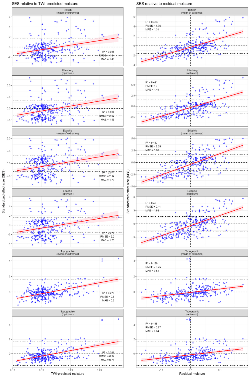
A contrasting pattern emerged for residual moisture, representing the component of moisture variation not explained by topography and therefore likely associated with local edaphic processes. In this case, the strongest relationships were observed for the edaphic scales (R² = 0.480–0.487), slightly exceeding those obtained for the traditional Didukh (R² = 0.433) and Ellenberg (R² = 0.421) scales. The topographic scales, by contrast, were only weakly related to residual moisture (R² = 0.118–0.136). Thus, the topographic indicators primarily captured the terrain-driven component of moisture variability, whereas the edaphic scales most effectively reflected the residual component of moisture conditions associated with local soil properties and microsite heterogeneity. Notably, most SES values remained within the neutral interval (−1.645 to 1.645), indicating that individual vegetation plots generally did not differ strongly from null-model expectations. Nevertheless, significant positive trends were observed along both the topographic and residual moisture gradients, suggesting that the ecological signal is expressed as a systematic directional shift in SES rather than as widespread strong deviations from the null expectation. This pattern implies that moisture gradients influence community assembly through cumulative changes in species composition, even when the majority of individual communities remain close to random expectations.
The SES diagnostics were used to compare alternative phytoindication scales intended to characterize the same ecological dimension, namely moisture conditions. In this framework, moisture indicator values were treated as functional traits of species. Positive deviations from random expectation were interpreted as divergence, potentially reflecting trait differentiation within communities and a greater role of biotic interactions mediated by moisture-related niche differences. Negative deviations were interpreted as convergence, indicating environmental filtering, that is, the selection of species with similar moisture preferences under particular site conditions. The Mayorka Valley data revealed remarkably similar patterns for the traditional and newly developed edaphic moisture indicators (Table 3).
Divergence accounted for 11.4% of observations for the Didukh scale, 12.1% for the Ellenberg scale, 13.5% for the edaphic mean-of-extremes scale, and 12.5% for the edaphic optimum scale. Likewise, convergence was consistently frequent across these indicators, comprising 22.1%, 30.4%, 30.8%, and 31.1% of observations, respectively. Thus, all four indicators identified comparable levels of both trait differentiation and environmental filtering, suggesting that they capture broadly similar aspects of moisture-related community assembly. In contrast, the topographic moisture indicators exhibited a fundamentally different pattern. Approximately 98% of observations fell within the neutral SES interval, whereas divergence accounted for only 1.4–1.7% of observations and convergence was virtually absent. This result indicates that the topographic indicators describe a moisture component that rarely produces strong deviations from null-model expectations, despite showing clear relationships with environmental gradients. Regression diagnostics further emphasized the distinction between edaphic and topographic indicators. For the TWI-predicted moisture component, divergence slopes were close to zero for the traditional and edaphic scales (−0.05 to 0.33), indicating only weak sensitivity to the topographically structured component of moisture variation. By contrast, the topographic mean-of-extremes scale exhibited a substantially stronger positive slope (1.97), suggesting that this indicator is particularly responsive to terrain-controlled moisture gradients. A different pattern emerged for residual moisture, representing the component of moisture variation not explained by topography and therefore likely associated with local soil conditions. Positive and significant divergence slopes were observed for all traditional and edaphic indicators (0.56–0.64), indicating increasing trait differentiation along the residual moisture gradient. However, the strongest response was observed for the topographic mean-of-extremes scale, which showed a pronounced negative slope (−3.78), implying a fundamentally different mode of response to residual moisture variation. The topographic optimum scale exhibited only a weak residual response (−0.44). The results suggest that the traditional, Ellenberg, and newly developed edaphic indicators describe largely the same moisture gradient and reveal similar patterns of community assembly. In contrast, the topographic indicators capture a distinct component of moisture variation associated with terrain structure. Rather than generating strong divergence or convergence patterns, this component appears to influence communities through gradual directional shifts in species composition, resulting in predominantly neutral SES values despite clear relationships with topographic moisture gradients.
In the floodplain ecosystems of Khortytsia Island, relationships between SES and TWI-predicted moisture were generally weak across all tested phytoindication scales (Figure 11). The highest explanatory power was observed for the Ellenberg optimum scale (R² = 0.107) and the edaphic optimum scale (R² = 0.110), whereas the Didukh and edaphic mean-of-extremes scales showed similarly weak associations (R² = 0.079 and 0.092, respectively). The topographic scales were only marginally related to TWI-predicted moisture (R² = 0.007 and 0.000). In contrast, substantially stronger relationships were observed for residual moisture, representing the component of NDWI variability not explained by TWI. The strongest responses were detected for the newly developed edaphic scales (R² = 0.259 and 0.265), followed by the Ellenberg (R² = 0.214) and Didukh (R² = 0.172) indicators. Topographic scales remained weakly related to residual moisture (R² = 0.051 and 0.037). This pattern indicates that moisture variation relevant for community assembly in the Khortytsia floodplain is driven primarily by edaphic and hydrological factors not captured by local topographic wetness indices. The stronger performance of the regional edaphic scales suggests that their calibration improves the representation of moisture conditions operating in floodplain ecosystems.
The SES diagnostics for the floodplain ecosystems of Khortytsia Island revealed a predominance of neutral community structure across all moisture indicators. Neutral observations accounted for 72.9–97.0% of cases, whereas convergence observations represented only 1.1–5.2% of communities. Divergence observations were more frequent than convergence for all indicators, but their proportion varied substantially among scales, from 1.7–4.0% for the topographic scales to 15.5–22.0% for the phytoindication and edaphic scales. The Ellenberg optimum scale showed the highest proportion of divergence observations (22.0%), followed by the edaphic optimum scale (20.5%), whereas the topographic scales yielded overwhelmingly neutral patterns. This indicates that species-based moisture indicators captured stronger differentiation in community structure than purely topographic scales.
Relationships with the TWI-predicted component of moisture were generally weak. Divergence slopes were close to zero across all indicators, ranging from −0.08 to 0.03. Significant positive convergence slopes were observed for the Didukh scale (0.26), the edaphic mean-of-extremes scale (0.24), and the edaphic optimum scale (0.19), whereas the topographic mean-of-extremes scale showed a negative convergence response (−0.52). Residual moisture also produced weak divergence responses, although the edaphic optimum scale showed a small positive slope (0.06). Convergence responses to residual moisture were strongest for the Didukh scale (0.25), while the other indicators showed weaker positive slopes. The Khortytsia floodplain was characterized by a largely neutral SES structure, with limited evidence for strong moisture-related community filtering. The edaphic and traditional phytoindication scales were more responsive than the topographic scales, but the observed relationships remained modest, suggesting that community assembly in these floodplain ecosystems reflects a complex hydrological regime that is only partly captured by TWI-derived moisture components.
In the sandy ecosystems of the first above-floodplain terrace of the Dnipro River, SES exhibited only weak relationships with the TWI-predicted component of moisture across all tested phytoindication scales (Figure 12). Coefficients of determination ranged from 0.030 to 0.050, indicating that topographically structured moisture variation explained only a small fraction of the observed variation in community assembly patterns. Even the newly developed topographic indicators showed only marginally stronger relationships than the traditional and edaphic scales. This pattern is consistent with the geomorphological setting of the sandy terrace, where relief is relatively subdued and local topographic redistribution of water contributes little to overall moisture heterogeneity. In contrast, SES was strongly associated with residual moisture, representing the component of moisture variation not explained by TWI and therefore likely linked to local edaphic conditions. Very high coefficients of determination were observed for the traditional and edaphic moisture indicators. The Didukh and Ellenberg scales yielded R² values of 0.812 and 0.793, respectively, while the newly developed edaphic mean-of-extremes and optimum scales showed the strongest relationships overall (R² = 0.834 and 0.833).
The near-identical responses of these four indicators suggest that they capture the same dominant environmental gradient governing community assembly in the sandy terrace ecosystems. The topographic indicators behaved differently. Although they also responded positively to residual moisture, their explanatory power was substantially lower (R² = 0.502 for the mean-of-extremes scale and R² = 0.449 for the optimum scale) than that of the traditional and edaphic indicators. Thus, while the topographic scales retain some sensitivity to moisture variation, they provide a less accurate representation of the principal moisture gradient operating in these ecosystems. The results indicate that moisture-related community assembly on the sandy terrace is governed predominantly by edaphic rather than topographic controls. The weak relationships with the TWI-predicted component and the consistently strong relationships with residual moisture suggest that local soil properties, rather than terrain-driven water redistribution, constitute the primary mechanism structuring moisture-related variation in plant communities.
The SES diagnostics for the sandy ecosystems of the first above-floodplain terrace revealed clear differences between the traditional and edaphic moisture indicators on the one hand and the topographic indicators on the other (Table 4). The traditional and edaphic scales showed broadly similar patterns of community assembly. Neutral observations accounted for 35.4–57.9% of cases, divergence for 13.8–32.9%, and convergence for 28.3–31.7%. The newly developed edaphic indicators exhibited the highest proportions of divergence (32.7–32.9%) and convergence (31.5–31.7%), indicating a strong sensitivity to both trait differentiation and environmental filtering processes. The Didukh scale yielded lower divergence (13.8%), whereas the Ellenberg scale occupied an intermediate position (23.8%). In contrast, the topographic indicators were dominated by neutral observations, which accounted for 84.3–87.1% of cases. Divergence was rare (1.9–3.9%), and convergence remained comparatively infrequent (10.9–11.8%). Thus, the topographic indicators detected substantially fewer departures from random expectations than either the traditional or the edaphic moisture scales. The TWI-predicted moisture component exhibited only weak relationships with SES patterns. Positive divergence slopes were observed for the Didukh (0.09), Ellenberg (0.08), and both edaphic scales (0.05), whereas the topographic indicators showed slopes close to zero (0.00 and −0.02). Convergence slopes were negligible for all indicators (−0.02 to 0.02). These results suggest that topographically structured moisture variation contributes little to community assembly in the sandy terrace ecosystems. A much stronger pattern emerged for residual moisture. Positive divergence slopes were observed for all traditional and edaphic indicators, reaching 0.24 for the Didukh scale and 0.21 for the Ellenberg scale, compared with 0.05 and 0.07 for the edaphic mean-of-extremes and optimum scales, respectively. Positive convergence slopes were also detected for these indicators, ranging from 0.06 to 0.15. In contrast, the topographic indicators showed little response to residual moisture, with slopes close to zero or slightly negative.
3.7. Cross-Validation of Moisture Indicator Scales
All analysed moisture scales showed a mutually consistent ordering of species moisture preferences, including the continuous traditional and newly developed phytoindication scales as well as the categorical-ordinal Belgard–Tarasov hygromorph classification (Figure 13). The newly developed edaphic moisture scales exhibited the strongest correspondence with the independent Belgard–Tarasov hygromorph classification (ρ = 0.69–0.70). Their correlations exceeded those observed for the traditional Ellenberg optimum scale (ρ = 0.66) and the Didukh minimum and maximum moisture values (ρ = 0.59–0.64). In contrast, the topographic moisture scales showed substantially weaker associations with the hygromorph score (ρ = 0.22–0.30). These results indicate that the edaphic scales most closely reproduce expert assessments of species moisture preferences, whereas the topographic scales represent a distinct moisture-related dimension that is only weakly reflected in the traditional hygromorph classification.
4. Discussion
4.1. Edaphic and Topographic Components of the Moisture Regime
The most important outcome of this study is the demonstration that the ecologically relevant moisture regime in the steppe zone of Ukraine cannot be adequately described by a single moisture gradient. Analysis of species distributions revealed the existence of at least two partially independent dimensions of moisture availability, each representing a different mechanism governing the formation of the water regime. Both dimensions were consistently associated with the climatic precipitation gradient, confirming the fundamental role of atmospheric water supply as the primary source of moisture for terrestrial ecosystems. However, the subsequent fate of this water is determined by different environmental processes. The first dimension was primarily associated with soil texture and its water-retention capacity. This finding is consistent with the widely accepted view that soil physical properties, particularly soil texture, are among the principal drivers of soil moisture dynamics because they regulate water retention, infiltration, hydraulic conductivity, and the amount of water available to plants [71]. It should be noted that soil texture also serves as a proxy for the variability of several other soil properties that collectively determine water-holding capacity, including organic matter content, soil profile depth, aggregate structure, bulk density, and related characteristics [13]. This gradient, therefore, reflects the contrast between substrates with high water-storage capacity and coarse-textured sandy soils, where water is rapidly lost through infiltration or evaporation. The traditional phytoindication moisture scales proved to be primarily sensitive to this component of the moisture regime. This finding suggests that the edaphic component of moisture availability most likely represents the aspect of the water regime that historically underpinned expert assessments of species ecological optima and tolerance ranges. The second dimension was determined predominantly by topographically driven water redistribution. It characterises the contrast between landscape positions that favour water accumulation and those dominated by drainage and runoff. Unlike the edaphic component, this gradient is only weakly captured by traditional phytoindication systems, although the present results demonstrate that it makes an independent contribution to plant community assembly. Recent studies have shown that similar climatic conditions may lead to different levels of ecosystem water availability because soil hydraulic properties strongly modulate the onset of water limitation [71]. Moreover, the relationship between precipitation and soil moisture is spatially heterogeneous and non-linear, being shaped not only by rainfall input but also by evapotranspiration, vegetation type, runoff, and soil properties [72]. The present findings extend this view by showing that plant communities respond differentially to the edaphic and topographic components of the moisture regime. Consequently, identical levels of climatic water input may yield different ecological outcomes. Under the same precipitation regime, plant communities may develop either on soils differing in water-retention capacity or on topographic surfaces with contrasting patterns of water redistribution. These findings indicate that moisture, as an ecological factor, is inherently multidimensional and that its representation by a single integrated gradient inevitably obscures part of the ecologically meaningful variation governing plant community composition.
4.2. Why Topographic Moisture Is Underrepresented in Traditional Phytoindication Scales
A key finding of this study is the asymmetric contribution of the two identified components of the water regime. The edaphic component explained a larger proportion of variation in plant responses and showed a close relationship with traditional phytoindication scales. The topographic component was also statistically significant, but its contribution was smaller and, more importantly, substantially more context-dependent. Unlike soil texture, which is a relatively stable property of a habitat, the effect of relief on the moisture regime is mediated by water redistribution processes whose intensity depends on weather conditions, precipitation amount and seasonality, and the spatial scale of analysis [73]. This interpretation is consistent with studies showing that topographic controls on soil moisture are state-dependent rather than constant [73]. The ecological effect of topographic water accumulation or drainage is not invariant [74,75], providing a mechanistic explanation for our finding that the same landform element may promote moisture accumulation under some hydrological conditions but have little effect, or even function primarily as a drainage pathway, under others. This context dependence probably explains why the topographic component is only weakly reflected in traditional phytoindication systems. Phytoindication scales are constructed as generalisations of stable patterns in species’ ecological behaviour over broad geographical ranges. Such generalisations naturally emphasise the most stable components of the environment, primarily those related to the substrate's water-retention capacity and the overall climatic moisture supply. By contrast, topographically driven variability is local in character and depends on the specific combination of climatic, geomorphological, and hydrological conditions. As a result, its signal is partly lost during the construction of generalised species-specific indicator values.
4.3. Phytoindication Reflects Realised Ecological Moisture Conditions Rather Than Single Hydrological Variables
The present results are fully consistent with previous studies demonstrating that the predictive value of topographic wetness metrics and phytoindication estimates increases substantially when information on soil water-holding capacity is incorporated. In particular, Petersson et al. [43] showed that including soil water capacity markedly improved the performance of both the Topographic Wetness Index and Ellenberg indicator values as predictors of site moisture conditions. This finding highlights the fundamental ecological importance of soil texture and related soil properties as determinants of the amount of water available to plants after precipitation events and topographic redistribution processes. The results obtained in the present study provide a conceptual explanation for this pattern. The analysis revealed that the dominant component of the moisture gradient perceived by vegetation is associated with the soil-mediated capacity of ecosystems to retain water, whereas topographic controls represent a secondary and more context-dependent source of variation. Consequently, information on soil texture contributes substantially to the ecological interpretation of moisture conditions beyond that provided by climatic or topographic variables alone. These findings also emphasise an important distinction between phytoindication and direct environmental measurements. The primary purpose of phytoindication is not to quantify moisture itself, but to characterise the biological response of vegetation to moisture conditions [37]. From this perspective, disagreement between phytoindication estimates and individual environmental variables should not necessarily be interpreted as a limitation of phytoindication. Rather, it reflects the fact that plant communities respond to the integrated effects of multiple environmental controls, including climatic inputs, soil water retention, groundwater influence, and topographic redistribution. Phytoindication, therefore, provides information on the realised ecological consequences of the water regime rather than on any single component of the hydrological system.
4.4. An Ecological Framework for Integrating Multiple Determinants of the Moisture Regime
A central contribution of this study is the demonstration that multiple abiotic determinants of the water regime can be integrated into ecologically meaningful moisture indices using vegetation itself as the calibration target. Previous approaches have generally considered climatic water supply, soil water-holding capacity, and topographic redistribution as independent components of the hydrological system [76,77]. In contrast, our approach integrates these processes within a single ecological framework by using plant community responses to identify the combinations of abiotic factors that best represent realised moisture conditions. An equally important distinction from traditional climatic moisture coefficients is that the proposed indices are not based solely on physical assumptions about the hydrological cycle. Instead, their mathematical structure was empirically calibrated against vegetation responses inferred from millions of species occurrence records and established phytoindication systems. Consequently, the regression coefficients represent empirically derived ecological relationships rather than predefined physical weights, allowing the indices to quantify moisture conditions in terms of their biological relevance for plant communities rather than only their physical hydrological characteristics.
A further important feature of the proposed indices is that they explicitly include interaction terms among the principal predictors. This is ecologically essential because precipitation, topographic wetness, and soil texture do not independently affect plant-available moisture. The same amount of precipitation may have very different ecological consequences depending on whether it falls on coarse- or fine-textured soils and whether a site is on a drained slope, a flat surface, or a topographically convergent position. Similarly, the effect of topographic water accumulation depends on the soil's capacity to retain this water and on the broader climatic context in which redistribution occurs. Such interactions are intuitively expected but difficult to derive analytically. The response of vegetation to the moisture regime is mediated by multiple processes, including infiltration, runoff, capillary rise, evaporation, soil water retention, rooting depth, and species-specific tolerance ranges. These processes are non-linear, scale-dependent, and partly compensatory. Therefore, a purely theoretical formulation of the combined effect of precipitation, relief, and soil texture would inevitably require strong simplifying assumptions. In this respect, the empirical approach used here provides a practical solution: it allows the interaction structure among abiotic predictors to be estimated directly from the realised vegetation response. The resulting formulae should not be interpreted simply as algebraic combinations of environmental variables. Rather, they represent empirically calibrated ecological summaries of how climatic water input, topographic redistribution, and soil-mediated retention jointly shape the moisture conditions experienced by plant communities. The inclusion of interaction terms is therefore not only a statistical refinement but also a necessary ecological component of the model. It reflects the fact that plant-available moisture arises from the combined, context-dependent action of several environmental controls, rather than from their additive effects alone.
4.5. Applying Edaphic and Topographic Moisture Indices to Mapping and Forecasting
An important implication of the proposed indices is that they can already be used to produce spatially explicit representations of moisture-regime variability in terms of abiotic predictors. By applying the fitted formulae to raster layers of precipitation, topographic wetness, and soil texture, it becomes possible to map edaphic and topographic components of moisture conditions across large territories. This has immediate value for ecological interpretation, vegetation analysis, and regional environmental assessment, because it translates separate climatic, geomorphological, and soil variables into ecologically calibrated moisture gradients. The significance of this approach extends beyond the current mapping of moisture conditions. It is also important for forecasting vegetation responses under climate change [78]. In most climate-change scenarios, precipitation is usually treated as the primary variable component of the water regime [79,80,81]. Yet changes in precipitation will not be translated into plant-available moisture uniformly across landscapes. The same climatic shift may produce different ecological consequences depending on local soil texture, water-retention capacity, and topographic position. Areas with fine-textured soils may buffer short-term reductions in precipitation more effectively than sandy substrates, while topographically convergent positions may retain or accumulate water even under drier regional conditions. Conversely, well-drained slopes and coarse-textured soils may experience stronger ecological drying under the same climatic scenario. The projections of future moisture conditions should not be based solely on precipitation changes. The real ecological effect of climate change on vegetation moisture regimes must be interpreted in the context of relief and soil properties. The proposed edaphic and topographic indices provide a practical framework for such interpretation. They allow changes in climatic water input to be translated into spatially differentiated estimates of ecologically relevant moisture availability, accounting for both soil capacity to retain water and terrain's capacity to redistribute it. This makes the indices potentially useful not only for present-day mapping but also for scenario-based assessment of future changes in plant habitats and vegetation structure.
4.6. Robustness of Traditional Phytoindication Scales and the Limited Effect of Local Recalibration
Local recalibration of indicator scales can improve their ecological performance, but the magnitude of this improvement was not large. The newly derived edaphic scale showed slightly higher consistency with several independent validation criteria, including reduced within-community variation for some moisture parameters, stronger correspondence with the Belgard–Tarasov hygromorph classification, and improved sensitivity to residual moisture gradients in local landscapes. However, these advantages were moderate rather than radical. In many cases, the traditional Didukh and Ellenberg moisture scales performed similarly to the locally calibrated edaphic scale. This result is important because it does not indicate a weakness of the traditional phytoindication systems. On the contrary, it confirms their broad ecological robustness. Despite being developed on the basis of expert knowledge and regional floristic experience, the Didukh and Ellenberg scales captured the dominant edaphic component of moisture variability over a wide geographical and ecological range. Therefore, local recalibration may be useful when higher spatial resolution or specific regional interpretation is required, but the traditional scales remain reliable tools for general ecological assessment. Thus, the proposed approach should be regarded not as a replacement for established phytoindication systems, but as a means of refining and decomposing them. It helps clarify which component of the moisture regime is primarily represented by traditional scales and where additional information can be obtained from locally calibrated or topographic indicators. The limited magnitude of improvement also supports the continued use of Didukh and Ellenberg indicator values in broad-scale vegetation studies, especially where direct recalibration is not possible or where comparability across regions is required.
4.7. Ecological Mechanisms Behind Phytoindication Performance
An important aspect of our results concerns the ecological mechanism underlying the indicator value of plant communities. The widespread use of phytoindication has been accompanied by the concern that its predictive performance may sometimes appear "too good to be true", because indicator values and community composition are not statistically independent. Zelený and Schaffers [82] demonstrated that part of this apparent explanatory power stems from compositional similarity rather than from environmental responses, and proposed randomisation procedures to separate these effects. Our randomisation analyses suggest that the ecological mechanisms underlying the indicator properties of plant communities differ across the investigated moisture indices. In some cases, the observed community structure was primarily consistent with environmental filtering, indicating that species composition directly reflects abiotic moisture conditions. In other cases, however, the observed deviation from the random expectation was more consistent with trait divergence, implying that interspecific competition and niche differentiation contributed substantially to the final community composition. Consequently, phytoindication reflects not only the direct action of environmental factors but also the ecological assembly processes operating within plant communities.
According to this criterion, the traditional Didukh and Ellenberg scales demonstrated a robust predominance of the environmental filtering mechanism, confirming their suitability as indicators of realised moisture conditions. The locally recalibrated edaphic scale performed slightly better, suggesting that local calibration increases the proportion of environmentally driven information while reducing the influence of stochastic or community-assembly effects. In contrast, the topographic moisture indicator exhibited a context-dependent pattern. Depending on local environmental settings, its indicator value could arise either predominantly from environmental filtering or from community assembly processes associated with trait divergence. This behaviour is consistent with the indirect nature of topographic controls, which influence plant water availability through interactions with soil properties, hydrological connectivity, and local landscape configuration rather than acting as direct ecological factors themselves.
5. Conclusions
This study addressed the problem by deriving empirically calibrated moisture indices that integrate climatic, edaphic, and topographic determinants of the water regime through the realised response of vegetation. These indices combine climatic water supply, soil water-retention properties, and topographic redistribution into comprehensive descriptors of the moisture conditions experienced by plant communities. The proposed indices were calibrated against the actual ecological responses of vegetation, thereby quantifying moisture conditions not only in physical terms but also in terms of their biological relevance to plants. The inclusion of interaction terms further underscores the inherently non-additive nature of moisture availability, in which the ecological effects of precipitation depend on both soil properties and topographic context. As such interactions arise from numerous coupled hydrological and ecological processes, they are challenging to derive analytically and are most effectively captured through empirical calibration. The resulting framework also demonstrates that the ecological moisture regime can be decomposed into complementary edaphic and topographic components. While both indices describe realised moisture conditions, they differ in their ecological interpretation and spatial behaviour, providing additional insight into the mechanisms governing plant responses to water availability. A significant advantage of this framework is its applicability not only to present-day ecological assessment but also to forecasting future changes in moisture conditions. Because the indices are expressed through measurable abiotic predictors, they can be mapped continuously across landscapes and readily incorporated into climate-change assessments. This enables future changes in precipitation to be translated into ecologically meaningful estimates of plant-available moisture while accounting for the modifying effects of soil properties and terrain. Consequently, the framework provides both a conceptual basis for understanding realised moisture conditions and a practical tool for ecological mapping and forecasting under changing environmental conditions.
Author Contributions
Conceptualization, O.K. and O.Z.; methodology, O.L.; software, H.T.; validation, O.K., O.L. and O.Z.; formal analysis, H.T.; investigation, O.L.; resources, O.Z.; data curation, H.T.; writing—original draft preparation, O.Z.; writing—review and editing, O.K.; visualization, O.L.; supervision, H.T.; project administration, O.L.; funding acquisition, O.Z. All authors have read and agreed to the published version of the manuscript.
Funding
This research was funded by National Research Foundation of Ukraine, grant number 2025.07/0001 “Procrustean analysis of spectral indices for assessing changes in hemeroby and the functional structure of plant communities as a result of military destruction: the example of the destruction of the Kakhovka Reservoir”.
Acknowledgments
The authors would like to express their sincere gratitude to the leadership of Bohdan Khmelnytskyi Melitopol State Pedagogical University for their administrative and technical support. The authors have reviewed and edited the output and take full responsibility for the content of this publication.
Conflicts of Interest
The authors declare no conflicts of interest.
References
- Chaves, M.M.; Maroco, J.P.; Pereira, J.S. Understanding Plant Responses to Drought — from Genes to the Whole Plant. Funct. Plant Biol. 2003, 30, 239–264. [CrossRef]
- Boyer, J.S. Plant Productivity and Environment. Science (80-. ). 1982, 218, 443–448. [CrossRef]
- Lambers, H.; Chapin, F.S.; Pons, T.L. Life Cycles: Environmental Influences and Adaptations. In Plant Physiological Ecology; Springer New York: New York, NY, 2008; pp. 375–402.
- Farquhar, G.D.; Sharkey, T.D. Stomatal Conductance and Photosynthesis. Annu. Rev. Plant Physiol. 1982, 33, 317–345. [CrossRef]
- Hudimov, M.I.; Zaitseva, I.O. Ecological Differentiation of Viburnum Species According to Their Resistance to Hydrothermal Stress Using Water Regime Indicators. Biosyst. Divers. 2026, 34, e2605. [CrossRef]
- Hetherington, A.M.; Woodward, F.I. The Role of Stomata in Sensing and Driving Environmental Change. Nature 2003, 424, 901–908. [CrossRef]
- Beerling, D.J.; Franks, P.J. The Hidden Cost of Transpiration. Nature 2010, 464, 495–496. [CrossRef]
- Kunakh, O.; Lisovets, O.; Tutova, H.; Zymaroieva, A.; Svenning, J.-C.; Zhukov, O. Functional Diversity Shifts and Ruderalisation of Floodplain in the Early Post-Disturbance Stage after Wartime Dam Destruction in Ukraine. Plant Ecol. 2026, 227, 64. [CrossRef]
- Seneviratne, S.I.; Corti, T.; Davin, E.L.; Hirschi, M.; Jaeger, E.B.; Lehner, I.; Orlowsky, B.; Teuling, A.J. Investigating Soil Moisture–Climate Interactions in a Changing Climate: A Review. Earth-Science Rev. 2010, 99, 125–161. [CrossRef]
- Vereecken, H.; Schnepf, A.; Hopmans, J.W.; Javaux, M.; Or, D.; Roose, T.; Vanderborght, J.; Young, M.H.; Amelung, W.; Aitkenhead, M.; et al. Modeling Soil Processes: Review, Key Challenges, and New Perspectives. Vadose Zo. J. 2016, 15, 1–57. [CrossRef]
- Rawls, W.J.; Pachepsky, Y.A.; Ritchie, J.C.; Sobecki, T.M.; Bloodworth, H. Effect of Soil Organic Carbon on Soil Water Retention. Geoderma 2003, 116, 61–76. [CrossRef]
- Minasny, B.; McBratney, A.B. Limited Effect of Organic Matter on Soil Available Water Capacity. Eur. J. Soil Sci. 2018, 69, 39–47. [CrossRef]
- Saxton, K.E.; Rawls, W.J. Soil Water Characteristic Estimates by Texture and Organic Matter for Hydrologic Solutions. Soil Sci. Soc. Am. J. 2006, 70, 1569–1578. [CrossRef]
- Canadell, J.; Jackson, R.B.; Ehleringer, J.B.; Mooney, H.A.; Sala, O.E.; Schulze, E.-D. Maximum Rooting Depth of Vegetation Types at the Global Scale. Oecologia 1996, 108, 583–595. [CrossRef]
- Dawson, T.E.; Ehleringer, J.R. Streamside Trees That Do Not Use Stream Water. Nature 1991, 350, 335–337. [CrossRef]
- Moore, I.D.; Grayson, R.B.; Ladson, A.R. Digital Terrain Modelling: A Review of Hydrological, Geomorphological, and Biological Applications. Hydrol. Process. 1991, 5, 3–30. [CrossRef]
- Western, A.W.; Grayson, R.B.; Blöschl, G. Scaling of Soil Moisture: A Hydrologic Perspective. Annu. Rev. Earth Planet. Sci. 2002, 30, 149–180. [CrossRef]
- Jenny, H. Factors of Soil Formation: A System of Quantitative Pedology; McGraw-Hill Book Company: New York, 1941.
- Pennock, D.J.; Zebarth, B.J.; De Jong, E. Landform Classification and Soil Distribution in Hummocky Terrain, Saskatchewan, Canada. Geoderma 1987, 40, 297–315. [CrossRef]
- Moore, I.D.; Gessler, P.E.; Nielsen, G.A.; Peterson, G.A. Soil Attribute Prediction Using Terrain Analysis. Soil Sci. Soc. Am. J. 1993, 57, 443–452. [CrossRef]
- Trenberth, K.E.; Fasullo, J.T.; Kiehl, J. Earth’s Global Energy Budget. Bull. Am. Meteorol. Soc. 2009, 90, 311–324. [CrossRef]
- Trenberth, K.E. Atmospheric Moisture Residence Times and Cycling: Implications for Rainfall Rates and Climate Change. Clim. Change 1998, 39, 667–694. [CrossRef]
- Hassanpour, B.; Richards, B.K.; Goehring, L.D.; Parlange, J.-Y.; Steenhuis, T.S. Predicting the Fate of Preferentially Moving Herbicides. Vadose Zo. J. 2019, 18, 1–11. [CrossRef]
- Beven, K.J.; Kirkby, M.J. A Physically Based, Variable Contributing Area Model of Basin Hydrology. Hydrol. Sci. Bull. 1979, 24, 43–69. [CrossRef]
- Kunakh, O.; Ivanko, I.; Holoborodko, K.; Lisovets, O.; Tutova, H.; Zhukov, O. Tree Stand Structure Drives Hemeroby and Naturalness, Jointly Shaping the Functional Diversity of the Herb Layer in Urban Parks. Biosyst. Divers. 2026, 34, e2601. [CrossRef]
- Ellenberg, H. Zeigerwerte Der Gefäßpflanzen Mitteleuropas (Indicator Values of Vascular Plants in Central Europe). Scr. Geobot. 1974, 9, 1–97. [CrossRef]
- Zhukov, O.; Kunakh, O. The Asymmetry of the Aquatic Macrophyte Response to Temperature Increases with Global Warming and Has to Be Accounted for in Phytoindication 2024.
- Didukh, Y.P. The Ecological Scales for the Species of Ukrainian Flora and Their Use in Synphytoindication; Kyiv, Phytosociocenter: Kyiv, 2011.
- Thornthwaite, C.W. An Approach toward a Rational Classification of Climate. Geogr. Rev. 1948, 38, 55. [CrossRef]
- Diekmann, M. Species Indicator Values as an Important Tool in Applied Plant Ecology - A Review. Basic Appl. Ecol. 2003, 4, 493–506. [CrossRef]
- Rösch, H.; Van Rooyen, M.W.; Theron, G.K. Predicting Competitive Interactions between Pioneer Plant Species by Using Plant Traits. J. Veg. Sci. 1997, 8, 489–494. [CrossRef]
- Vicente-Serrano, S.M.; Beguería, S.; López-Moreno, J.I. A Multiscalar Drought Index Sensitive to Global Warming: The Standardized Precipitation Evapotranspiration Index. J. Clim. 2010, 23, 1696–1718. [CrossRef]
- Schaffers, A.P.; Sýkora, K. V. Reliability of Ellenberg Indicator Values for Moisture, Nitrogen and Soil Reaction: A Comparison with Field Measurements. J. Veg. Sci. 2000, 11, 225–244. [CrossRef]
- Tichý, L.; Axmanová, I.; Dengler, J.; Guarino, R.; Jansen, F.; Midolo, G.; Nobis, M.P.; Van Meerbeek, K.; Aćić, S.; Attorre, F.; et al. Ellenberg-type Indicator Values for European Vascular Plant Species. J. Veg. Sci. 2023, 34. [CrossRef]
- Tutova, H.; Lisovets, O.; Kunakh, O.; Zhukov, O. From Species Traits to Community Gradients: Validation of Borhi-Di-like Naturalness Indicators in Steppe Vegetation. Biosyst. Divers. 2026, 34, e2608. [CrossRef]
- Tutova, H.; Panchenko, K.; Lisovets, O.; Kunakh, O.; Zhukov, O. Vegetation Diversity and Ecological Factor Assessment via Phytoindication on the Arena Terrace of the Dnipro Valley. Regul. Mech. Biosyst. 2025, 16, e25131. [CrossRef]
- Tutova, H.; Lisovets, O.; Kunakh, O.; Zhukov, O. Phytoindication Is a Useful Tool for Assessing the Response of Plant Communities to Environmental Factors. Diversity 2025, 17, 738. [CrossRef]
- Kopecký, M.; Hederová, L.; Macek, M.; Klinerová, T.; Wild, J. Forest Plant Indicator Values for Moisture Reflect Atmospheric Vapour Pressure Deficit Rather than Soil Water Content. New Phytol. 2024, 244, 1801–1811. [CrossRef]
- Hill, M.O.; Roy, D.B.; Mountford, J.O.; Bunce, R.G.H. Ellenberg’s Indicator Values for British Plants; Institute of Terrestrial Ecology: Huntingdon, United Kingdom, 1999.
- Schaffers, A.P.; Sýkora, K. V. Reliability of Ellenberg Indicator Values for Moisture, Nitrogen and Soil Reaction: A Comparison with Field Measurements. J. Veg. Sci. 2000, 11, 225–244. [CrossRef]
- Ertsen, A.C.D.; Alkemade, J.R.M.; Wassen, M.J. Calibrating Ellenberg Indicator Values for Moisture, Acidity, Nutrient Availability and Salinity in the Netherlands. Plant Ecol. 1998, 135, 113–124. [CrossRef]
- Sun, Y.; Sun, Y.; Yao, S.; Akram, M.A.; Hu, W.; Dong, L.; Li, H.; Wei, M.; Gong, H.; Xie, S.; et al. Impact of Climate Change on Plant Species Richness across Drylands in China: From Past to Present and into the Future. Ecol. Indic. 2021, 132, 108288. [CrossRef]
- Dwyer, C.; Millett, J.; Pakeman, R.J.; Jones, L. Environmental Modifiers of the Relationship between Water Table Depth and Ellenberg’s Indicator of Soil Moisture. Ecol. Indic. 2021, 132, 108320. [CrossRef]
- Schmidtlein, S.; Ewald, J. Landscape Patterns of Indicator Plants for Soil Acidity in the Bavarian Alps. J. Biogeogr. 2003, 30, 1493–1503. [CrossRef]
- Hájek, M.; Roleček, J.; Cottenie, K.; Kintrová, K.; Horsák, M.; Poulíčková, A.; Hájková, P.; Fránková, M.; Dítě, D. Environmental and Spatial Controls of Biotic Assemblages in a Discrete Semi-Terrestrial Habitat: Comparison of Organisms with Different Dispersal Abilities Sampled in the Same Plots. J. Biogeogr. 2011, 38, 1683–1693. [CrossRef]
- Wamelink, G.W.W.; Joosten, V.; van Dobben, H.F.; Berendse, F. Validity of Ellenberg Indicator Values Judged from Physico-chemical Field Measurements. J. Veg. Sci. 2002, 13, 269–278. [CrossRef]
- Raduła, M.W.; Szymura, T.H.; Szymura, M. Topographic Wetness Index Explains Soil Moisture Better than Bioindication with Ellenberg’s Indicator Values. Ecol. Indic. 2018, 85, 172–179. [CrossRef]
- Möckel, T.; Löfgren, O.; Prentice, H.C.; Eklundh, L.; Hall, K. Airborne Hyperspectral Data Predict Ellenberg Indicator Values for Nutrient and Moisture Availability in Dry Grazed Grasslands within a Local Agricultural Landscape. Ecol. Indic. 2016, 66, 503–516. [CrossRef]
- Di Biase, L.; Tsafack, N.; Pace, L.; Fattorini, S. Ellenberg Indicator Values Disclose Complex Environmental Filtering Processes in Plant Communities along an Elevational Gradient. Biology (Basel). 2023, 12, 161. [CrossRef]
- Schmidtlein, S. Imaging Spectroscopy as a Tool for Mapping Ellenberg Indicator Values. J. Appl. Ecol. 2005, 42, 966–974. [CrossRef]
- Tarasov, V.V. Flora of Dnipropetrovsk and Zaporizhia Regions; Travleev, A.P., Ed.; Lira (in Ukranian): Dnipropetrovsk, 2012.
- Ellenberg, H. Zeigerwerte Der Gefasspflanzen Mitteleuropas. In Scripta geobotanica, 9; Gottingen, 1974; pp. 1–197.
- Dengler, J.; Jansen, F.; Chusova, O.; Hüllbusch, E.; Nobis, M.P.; Van Meerbeek, K.; Axmanová, I.; Bruun, H.H.; Chytrý, M.; Guarino, R.; et al. Ecological Indicator Values for Europe (EIVE) 1.0. Veg. Classif. Surv. 2023, 4, 7–29. [CrossRef]
- Zhukov, O.; Lisovets, O.; Molozhon, K. Differential Ecomorphic Analysis of Urban Park Vegetation. IOP Conf. Ser. Earth Environ. Sci. 2023, 1254, 1–21. [CrossRef]
- GBIF.org European Occurrence Records of Vascular Plant Species Filtered for Ecological Analysis 2026.
- Tutova, H.; Lisovets, O.; Kunakh, O.; Zhukov, O. European GBIF Occurrence Records of Vascular Plant Species from the Regional Flora of Dnipropetrovsk and Zaporizhzhia Regions, Ukraine. Zenodo 2026.
- Chamberlain, S.; Barve, V.; Mcglinn, D.; Oldoni, D.; Desmet, P.; Geffert, L.; Ram, K. _rgbif. Interface to Glob. Biodivers. Inf. Facil. API_. R Packag. version 3.7.9, <https//CRAN.R-project.org/package=rgbif> 2024.
- Ho, Y.; Hengl, T. Multiscale Land Surface Parameters of GEDTM30: Topographic Wetness Index (Version V20241230) [Data Set. Zenodo. [CrossRef]
- Fick, S.E.; Hijmans, R.J. WorldClim 2: New 1-Km Spatial Resolution Climate Surfaces for Global Land Areas. Int. J. Climatol. 2017, 37, 4302–4315. [CrossRef]
- Hijmans, R.J.; Barbosa, M.; Ghosh, A.; Mandel, A. Geodata: Download Geographic Data. R Packag. version 0.6-2 2024, 2, 1–32.
- Poggio, L.; de Sousa, L.M.; Batjes, N.H.; Heuvelink, G.B.M.; Kempen, B.; Ribeiro, E.; Rossiter, D. SoilGrids 2.0: Producing Soil Information for the Globe with Quantified Spatial Uncertainty. SOIL 2021, 7, 217–240. [CrossRef]
- Legendre, P.; Legendre, L. Canonical Analysis. Dev. Environ. Model. 2012, 24, 625–710. [CrossRef]
- Tutova, H.; Lisovets, O.; Kunakh, O.; Zhukov, O. Ecological Characteristics of Vascular Plants of the Dnipropetrovsk and Zaporizhzhia Regions (Ukraine): Ellenberg, Didukh, Edaphic, and Topographic Moisture Indicators 2026.
- Oksanen, J.; Blanchet, F.G.; Kindt, R.; Legendre, P.; Minchin, P.R.; O’Hara, R.B.; Simpson, G.L.; Solymos, P.; Stevens, M.H.H.; Wagner, H. Community Ecology Package. R Package Version 2.5-2. 2018.
- Lisovets, O.; Tutova, H.; Kunakh, O.; Zhukov, O. Plant Survey Data from Khortytsia Island (Ukraine), 2025 2025.
- Lisovets, O.; Tutova, H.; Kunakh, O.; Zhukov, O. Flora of the Arena (First Floodplain Terrace) of the Dnipro River Valley within the Dniprovsky-Orilskyi Nature Reserve (Ukraine) 2025.
- Tutova, H.; Lisovets, O.; Kunakh, O.; Zhukov, O. Occurrence Records of Vascular Plants from Steppe Gully Systems (Mayorska Valley, Dnipropetrovsk Region, Ukraine, 2023). Version 1.1. Bohdan Khmelnytsky Melitopol State Pedagog. Univ. Occur. dataset 2025 accessed via GBIF.org on 2025-09-06. [CrossRef]
- Lindsay, J.B. Whitebox GAT: A Case Study in Geomorphometric Analysis. Comput. Geosci. 2016, 95, 75–84. [CrossRef]
- Gao, B. NDWI—A Normalized Difference Water Index for Remote Sensing of Vegetation Liquid Water from Space. Remote Sens. Environ. 1996, 58, 257–266. [CrossRef]
- Ulrich, W. Species Co-Occurrences and Neutral Models: Reassessing J. M. Diamond’s Assembly Rules. Oikos 2004, 107, 603–609. [CrossRef]
- Wankmüller, F.J.P.; Delval, L.; Lehmann, P.; Baur, M.J.; Cecere, A.; Wolf, S.; Or, D.; Javaux, M.; Carminati, A. Global Influence of Soil Texture on Ecosystem Water Limitation. Nature 2024, 635, 631–638. [CrossRef]
- Xue, S.; Wu, G. A Study of the Dependence between Soil Moisture and Precipitation in Different Ecoregions of the Northern Hemisphere. Hydrol. Earth Syst. Sci. 2025, 29, 5575–5591. [CrossRef]
- Zignol, F.; Lidberg, W.; Greiser, C.; Larson, J.; Hoffrén, R.; Ågren, A.M. Controls on Spatial and Temporal Variability of Soil Moisture across a Heterogeneous Boreal Forest Landscape. Hydrol. Earth Syst. Sci. 2025, 29, 5493–5513. [CrossRef]
- Winzeler, H.E.; Owens, P.R.; Read, Q.D.; Libohova, Z.; Ashworth, A.; Sauer, T. Topographic Wetness Index as a Proxy for Soil Moisture in a Hillslope Catena: Flow Algorithms and Map Generalization. Land 2022, 11, 2018. [CrossRef]
- Coleman, M.L.; Niemann, J.D. Controls on Topographic Dependence and Temporal Instability in Catchment-scale Soil Moisture Patterns. Water Resour. Res. 2013, 49, 1625–1642. [CrossRef]
- Khomiak, I. V.; Onyshchuk, I.P.; Vakerych, M.M.; Hasynets, Y.S.; Schwartau, V. V. Restoration of Floodplains’ Natural Vegetation of Polissia to Reduce the Effects of Climate Change. Biosyst. Divers. 2025, 33, e2551. [CrossRef]
- Minarchenko, V.; Tymchenko, I.; Pushkarova, Y.; Dvirna, T.; Futorna, O.; Polishchuk, O. Impact of Climate Change on Populations and Resources of Convallaria Majalis. Biosyst. Divers. 2025, 33, e2543. [CrossRef]
- Chetvertak, T.; Diuzhykova, T.; Hryshko, S.; Nepsha, O.; Tutova, H. The Precipitation Levels during the Warmest Quarter Are the Primary Factor Influencing the Spatial Distribution of Opatrum Sabulosum. Biosyst. Divers. 2025, 33, e2507. [CrossRef]
- Nykytiuk, Y.; Kravchenko, O.; Komorna, О. Bioclimatic and Soil Determinants of Buckwheat Cultivation Prospects under Global Warming: A Case Study of the Ukrainian Polissya and Forest-Steppe. Biosyst. Divers. 2025, 33, e2537. [CrossRef]
- Nykytiuk, Y.; Kravchenko, O.; Vyskushenko, D.; Pitsil, A.; Komorna, O.; Bezvershuck, I. Bioclimatic Constraints and Edaphic Preferences of Wheat: Implications for Environmental Suitability Forecasting under Climate Change. Stud. Biol. 2025, 19, 137–156. [CrossRef]
- Nykytiuk, Y.; Kravchenko, O. Maize Response Patterns to Soil and Climate Factors Form the Basis for Predicting Changes in Its Growing Conditions under Climate Change. Biosyst. Divers. 2025, 33, e2553. [CrossRef]
- Zelený, D.; Schaffers, A.P. Too Good to Be True: Pitfalls of Using Mean Ellenberg Indicator Values in Vegetation Analyses. J. Veg. Sci. 2012, 23, 419–431. [CrossRef]
Figure 1.
Spatial distribution across Europe of GBIF occurrence records for plant species included in the flora of the Dnipropetrovsk and Zaporizhzhia regions of Ukraine. The dataset comprised 1,969 vascular plant species and 13,229,946 GBIF occurrence records. Records were thinned to a single occurrence per species within each 10 × 10 km grid cell to reduce spatial sampling bias, resulting in 4,707,830 unique species-grid records. Colours indicate the logarithmically transformed density of unique occurrences, log10(1 + number of occurrences). Major European biogeographical regions are shown for reference. The red outline indicates the reference region in southeastern Ukraine.
Figure 1.
Spatial distribution across Europe of GBIF occurrence records for plant species included in the flora of the Dnipropetrovsk and Zaporizhzhia regions of Ukraine. The dataset comprised 1,969 vascular plant species and 13,229,946 GBIF occurrence records. Records were thinned to a single occurrence per species within each 10 × 10 km grid cell to reduce spatial sampling bias, resulting in 4,707,830 unique species-grid records. Colours indicate the logarithmically transformed density of unique occurrences, log10(1 + number of occurrences). Major European biogeographical regions are shown for reference. The red outline indicates the reference region in southeastern Ukraine.
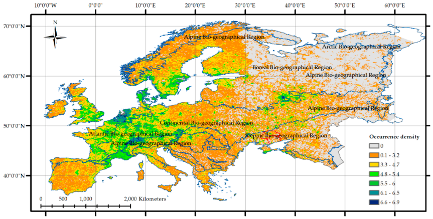
Figure 2.
Spatial distribution of vegetation plots used for validation of the moisture indicator scales (n = 10,931). The red outline delineates the focal regions of the Ukrainian steppe zone, encompassing the Dnipropetrovsk and Zaporizhzhia regions. Additional plots from the steppe part of the Donetsk region were included to improve the regional coverage of the validation dataset.
Figure 2.
Spatial distribution of vegetation plots used for validation of the moisture indicator scales (n = 10,931). The red outline delineates the focal regions of the Ukrainian steppe zone, encompassing the Dnipropetrovsk and Zaporizhzhia regions. Additional plots from the steppe part of the Donetsk region were included to improve the regional coverage of the validation dataset.
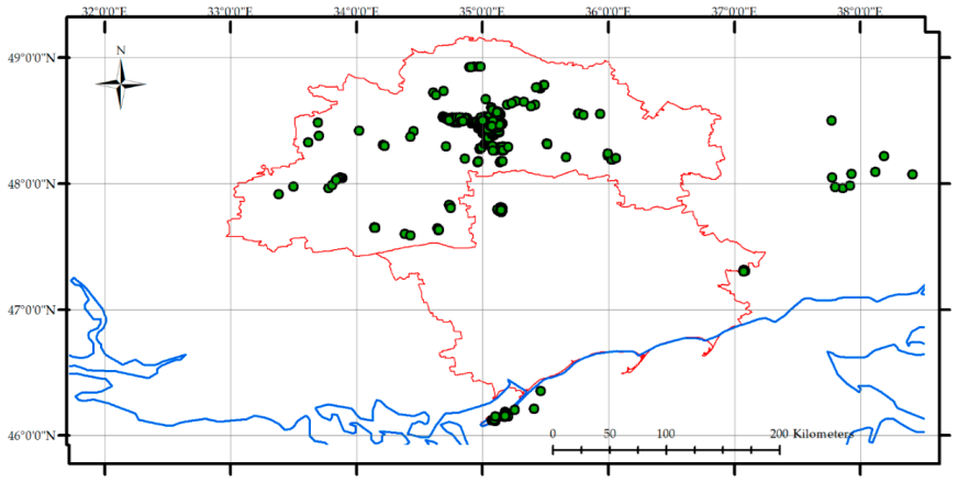
Figure 3.
Spatial distribution of vegetation plots within the three landscape systems used for local-scale validation of moisture indicator scales. Upper panel: psammophytic steppe landscape. Lower left panel: Mayorka Valley ravine–valley landscape system. Lower right panel: floodplain ecosystem complex of Khortytsia Island. Orange circles indicate vegetation plot locations. Red polygons delineate the boundaries of the analysed landscape systems. Background colours represent elevation derived from digital elevation models (DEM). The three landscapes encompass contrasting geomorphological and hydrological settings and were used to evaluate the performance of traditional and newly developed moisture indicator scales under local environmental conditions.
Figure 3.
Spatial distribution of vegetation plots within the three landscape systems used for local-scale validation of moisture indicator scales. Upper panel: psammophytic steppe landscape. Lower left panel: Mayorka Valley ravine–valley landscape system. Lower right panel: floodplain ecosystem complex of Khortytsia Island. Orange circles indicate vegetation plot locations. Red polygons delineate the boundaries of the analysed landscape systems. Background colours represent elevation derived from digital elevation models (DEM). The three landscapes encompass contrasting geomorphological and hydrological settings and were used to evaluate the performance of traditional and newly developed moisture indicator scales under local environmental conditions.
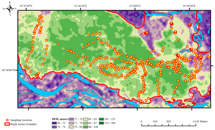
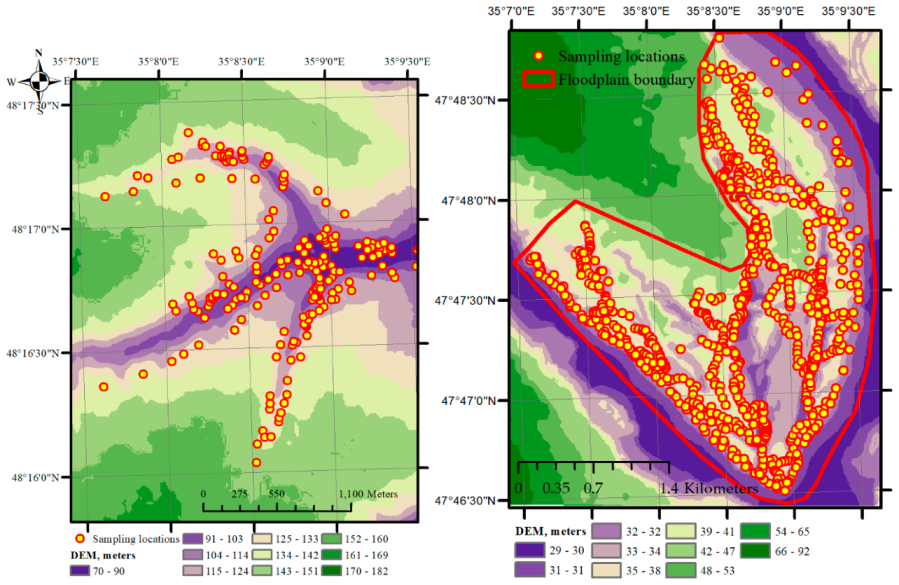
Figure 4.
Relationships of ecological moisture indicator values and CCA ordination scores with climatic, topographic and edaphic predictors. Scatterplots show the relationships between phytoindication moisture scales (Didukh minimum, Didukh maximum and Ellenberg F values), as well as CCA1 and CCA2 vegetation-composition scores, and three environmental predictors: log-transformed annual precipitation, topographic wetness index (TWI) and soil texture coefficient. Blue lines indicate linear regression fits, and panels display coefficients of determination (R²). The results demonstrate that phytoindication moisture values are positively associated with precipitation and TWI, and negatively associated with soil texture. In contrast, CCA1 scores are strongly related to soil texture, whereas CCA2 scores primarily reflect variation associated with topographic wetness.
Figure 4.
Relationships of ecological moisture indicator values and CCA ordination scores with climatic, topographic and edaphic predictors. Scatterplots show the relationships between phytoindication moisture scales (Didukh minimum, Didukh maximum and Ellenberg F values), as well as CCA1 and CCA2 vegetation-composition scores, and three environmental predictors: log-transformed annual precipitation, topographic wetness index (TWI) and soil texture coefficient. Blue lines indicate linear regression fits, and panels display coefficients of determination (R²). The results demonstrate that phytoindication moisture values are positively associated with precipitation and TWI, and negatively associated with soil texture. In contrast, CCA1 scores are strongly related to soil texture, whereas CCA2 scores primarily reflect variation associated with topographic wetness.
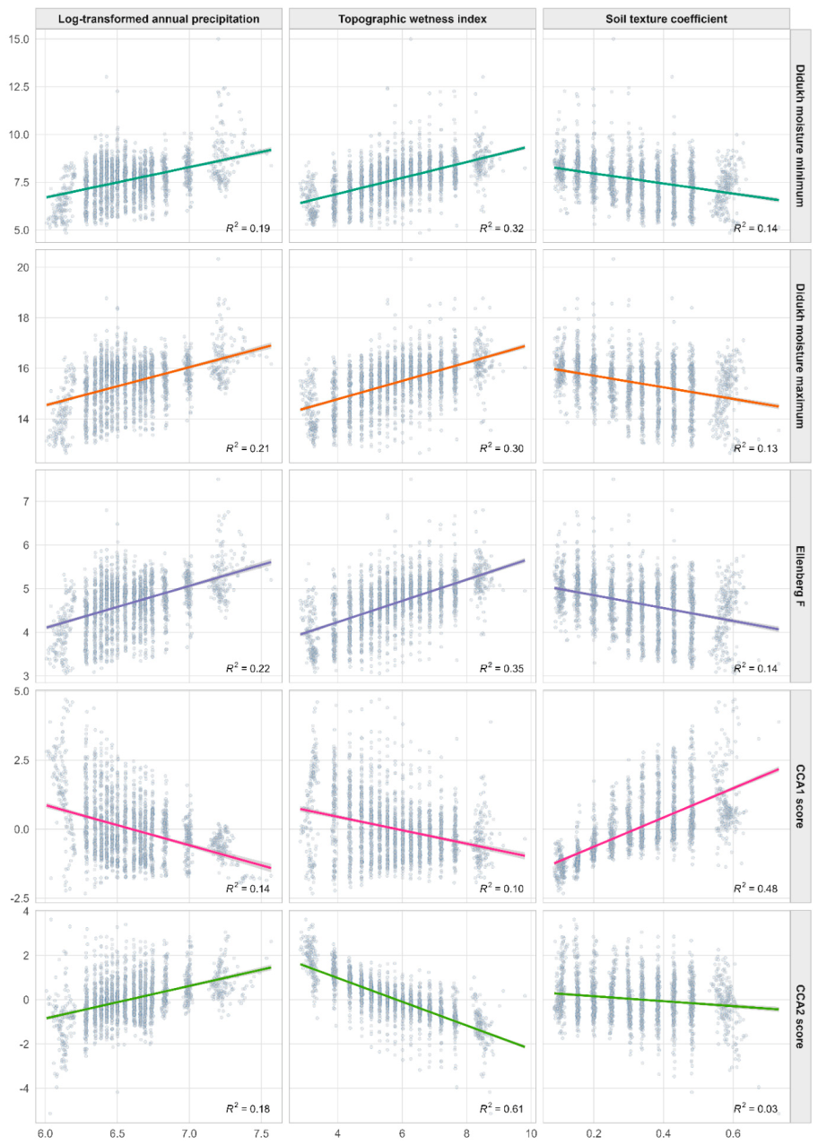
Figure 5.
Spatial distribution of the rescaled edaphic and topographic moisture gradients across southeastern Ukraine. The upper panel shows the edaphic moisture gradient, whereas the lower panel shows the topographic moisture gradient. Both gradients were derived from environmental predictors through canonical correspondence analysis and subsequent regression modelling and were recalibrated to the 1–23 numerical range of the Didukh ecological indicator system. Higher values indicate wetter environmental conditions, while lower values correspond to drier conditions. Red outlines delineate the focal study regions used for calibration and validation of the indicator scales. Boundaries of the Black Sea, Continental, and Steppe biogeographical regions are shown for geographic reference.
Figure 5.
Spatial distribution of the rescaled edaphic and topographic moisture gradients across southeastern Ukraine. The upper panel shows the edaphic moisture gradient, whereas the lower panel shows the topographic moisture gradient. Both gradients were derived from environmental predictors through canonical correspondence analysis and subsequent regression modelling and were recalibrated to the 1–23 numerical range of the Didukh ecological indicator system. Higher values indicate wetter environmental conditions, while lower values correspond to drier conditions. Red outlines delineate the focal study regions used for calibration and validation of the indicator scales. Boundaries of the Black Sea, Continental, and Steppe biogeographical regions are shown for geographic reference.
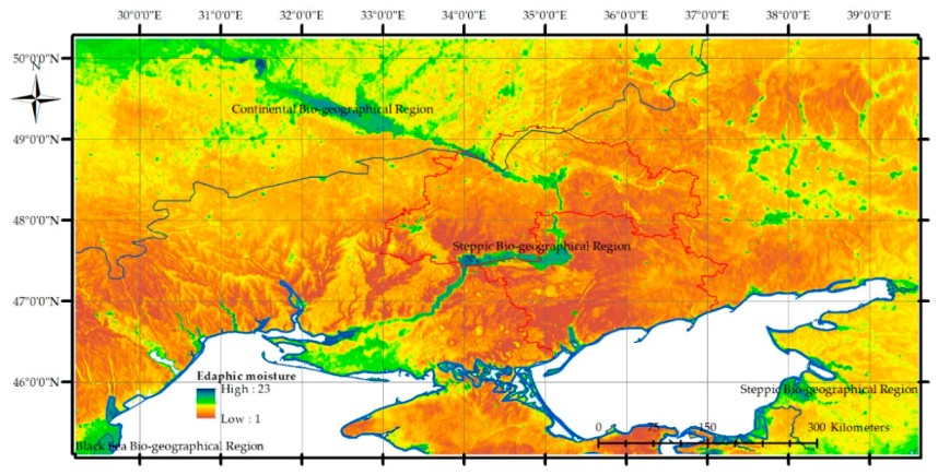
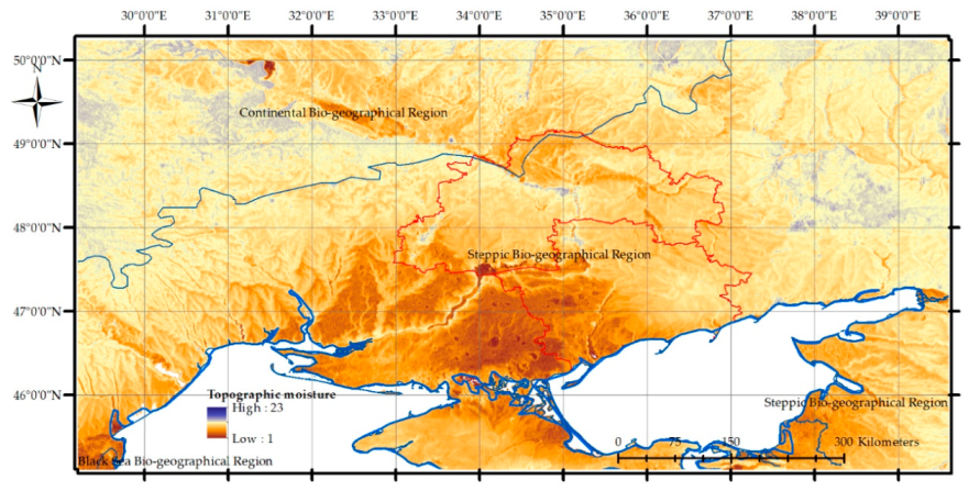
Figure 6.
Relationships between traditional moisture indicator values and the CCA-derived moisture gradients. The upper panels show comparisons between the edaphic moisture scale and the corresponding traditional indicators (Didukh minimum moisture, Ellenberg moisture optimum, and Didukh maximum moisture), whereas the lower panels show analogous comparisons for the topographic moisture scale. Red curves represent principal curves fitted to visualize the dominant non-linear trend in the data. The edaphic moisture scale exhibits a strong but distinctly non-linear correspondence with the traditional indicator systems, while the topographic moisture scale shows little association with existing phytoindication values, indicating that it captures an independent component of moisture variability not represented by conventional moisture indicators.
Figure 6.
Relationships between traditional moisture indicator values and the CCA-derived moisture gradients. The upper panels show comparisons between the edaphic moisture scale and the corresponding traditional indicators (Didukh minimum moisture, Ellenberg moisture optimum, and Didukh maximum moisture), whereas the lower panels show analogous comparisons for the topographic moisture scale. Red curves represent principal curves fitted to visualize the dominant non-linear trend in the data. The edaphic moisture scale exhibits a strong but distinctly non-linear correspondence with the traditional indicator systems, while the topographic moisture scale shows little association with existing phytoindication values, indicating that it captures an independent component of moisture variability not represented by conventional moisture indicators.
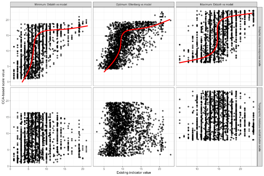
Figure 7.
Relative within-location variability of moisture indicator values for the traditional, edaphic and topographic moisture scales. Variability was calculated as the ratio of the within-location weighted standard deviation to the total species-level standard deviation of the corresponding scale. Boxplots show the distribution of relative variability across 10931 vegetation plots for minimum, optimum and maximum moisture indicator values. Lower values indicate greater within-community consistency of indicator values.
Figure 7.
Relative within-location variability of moisture indicator values for the traditional, edaphic and topographic moisture scales. Variability was calculated as the ratio of the within-location weighted standard deviation to the total species-level standard deviation of the corresponding scale. Boxplots show the distribution of relative variability across 10931 vegetation plots for minimum, optimum and maximum moisture indicator values. Lower values indicate greater within-community consistency of indicator values.
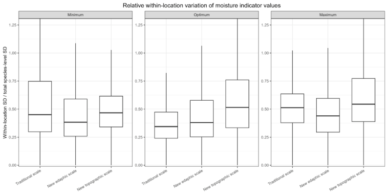
Figure 8.
Relationships between raster-derived edaphic moisture gradient and community-level phytoindication estimates calculated from vegetation plots. Phytoindication estimates were derived as abundance-weighted means of species indicator values using the traditional Didukh and Ellenberg moisture scales, the newly developed edaphic moisture scale, and the topographic moisture scale. Spearman rank correlation coefficients and 95% confidence intervals are shown for each comparison. Positive correlations observed for the traditional and edaphic indicators indicate agreement between the mapped edaphic moisture gradient and moisture conditions inferred from species composition. In contrast, the negative correlations observed for the topographic moisture indicators suggest that the topographic moisture gradient captures an environmental component distinct from the edaphic moisture conditions represented by conventional phytoindication systems.
Figure 8.
Relationships between raster-derived edaphic moisture gradient and community-level phytoindication estimates calculated from vegetation plots. Phytoindication estimates were derived as abundance-weighted means of species indicator values using the traditional Didukh and Ellenberg moisture scales, the newly developed edaphic moisture scale, and the topographic moisture scale. Spearman rank correlation coefficients and 95% confidence intervals are shown for each comparison. Positive correlations observed for the traditional and edaphic indicators indicate agreement between the mapped edaphic moisture gradient and moisture conditions inferred from species composition. In contrast, the negative correlations observed for the topographic moisture indicators suggest that the topographic moisture gradient captures an environmental component distinct from the edaphic moisture conditions represented by conventional phytoindication systems.
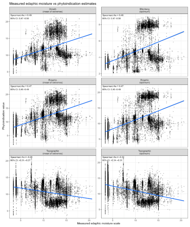
Figure 9.
Relationships between the raster-derived topographic moisture gradient and community-level phytoindication estimates calculated from vegetation plots. The topographic moisture gradient was derived from environmental predictors describing topographically mediated moisture redistribution and represents an environmental rather than vegetation-based estimate. Community-level phytoindication estimates were calculated as abundance-weighted means of species indicator values. Spearman rank correlation coefficients and 95% confidence intervals are shown for each comparison.
Figure 9.
Relationships between the raster-derived topographic moisture gradient and community-level phytoindication estimates calculated from vegetation plots. The topographic moisture gradient was derived from environmental predictors describing topographically mediated moisture redistribution and represents an environmental rather than vegetation-based estimate. Community-level phytoindication estimates were calculated as abundance-weighted means of species indicator values. Spearman rank correlation coefficients and 95% confidence intervals are shown for each comparison.
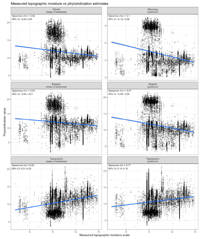
Figure 11.
Relationships between standardized effect size (SES) and TWI-predicted moisture (left) and residual moisture (right) for different phytoindication moisture scales in the floodplain ecosystems of Khortytsia Island. Dashed and dot-dashed lines indicate SES thresholds used to define neutral and non-neutral observations. For each scale, the coefficient of determination (R²), root mean square error (RMSE), and mean absolute error (MAE) are shown.
Figure 11.
Relationships between standardized effect size (SES) and TWI-predicted moisture (left) and residual moisture (right) for different phytoindication moisture scales in the floodplain ecosystems of Khortytsia Island. Dashed and dot-dashed lines indicate SES thresholds used to define neutral and non-neutral observations. For each scale, the coefficient of determination (R²), root mean square error (RMSE), and mean absolute error (MAE) are shown.
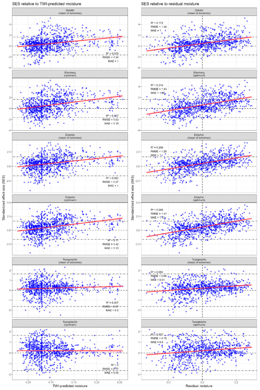
Figure 12.
Relationships between standardized effect size (SES) and TWI-predicted moisture (left) and residual moisture (right) for different phytoindication moisture scales in the sandy ecosystems of the first above-floodplain terrace of the Dnipro River. Dashed and dot-dashed lines indicate SES thresholds used to define neutral and non-neutral observations. For each scale, the coefficient of determination (R²), root mean square error (RMSE), and mean absolute error (MAE) are shown.
Figure 12.
Relationships between standardized effect size (SES) and TWI-predicted moisture (left) and residual moisture (right) for different phytoindication moisture scales in the sandy ecosystems of the first above-floodplain terrace of the Dnipro River. Dashed and dot-dashed lines indicate SES thresholds used to define neutral and non-neutral observations. For each scale, the coefficient of determination (R²), root mean square error (RMSE), and mean absolute error (MAE) are shown.
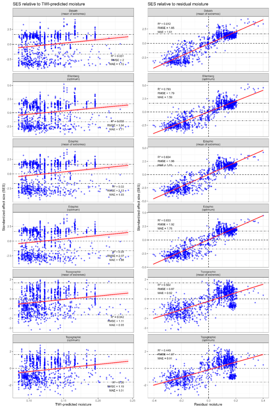
Figure 13.
Relationships between Belgard–Tarasov hygromorph categories and phytoindication moisture scales. Species-level moisture indicator values are plotted against the alternative expert hygromorph score. The Belgard–Tarasov hygromorph classes are ordered from 1 to 10: 1 — EuXero, euxerophyte; 2 — Xero, xerophyte; 3 — MsXero, meso-xerophyte; 4 — XeroMs, xero-mesophyte; 5 — Ms, mesophyte; 6 — HgMs, hygro-mesophyte; 7 — MsHg, meso-hygrophyte; 8 — Hg, hygrophyte; 9 — Pl, pleustophyte; 10 — Hy, hydatophyte. Blue lines represent linear regression fits with 95% confidence intervals. Spearman’s rank correlation coefficient (ρ) is shown in each panel.
Figure 13.
Relationships between Belgard–Tarasov hygromorph categories and phytoindication moisture scales. Species-level moisture indicator values are plotted against the alternative expert hygromorph score. The Belgard–Tarasov hygromorph classes are ordered from 1 to 10: 1 — EuXero, euxerophyte; 2 — Xero, xerophyte; 3 — MsXero, meso-xerophyte; 4 — XeroMs, xero-mesophyte; 5 — Ms, mesophyte; 6 — HgMs, hygro-mesophyte; 7 — MsHg, meso-hygrophyte; 8 — Hg, hygrophyte; 9 — Pl, pleustophyte; 10 — Hy, hydatophyte. Blue lines represent linear regression fits with 95% confidence intervals. Spearman’s rank correlation coefficient (ρ) is shown in each panel.
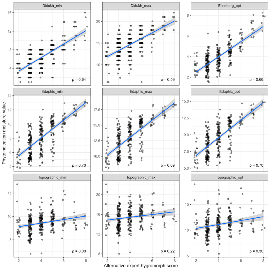

Table 1.
Constrained predictors and fitted moisture vectors in the CCA space.
| Predictor | CCA1 | CCA2 | |
|---|---|---|---|
| Constrained | Precipitation (P) | –0.29 | 0.70 |
| Topographic wetness index (TWI) | –0.41 | –0.87 | |
| Texture coefficient (TC) | 0.80 | 0.00 | |
| P × TWI | –0.60 | –0.10 | |
| P × C | 0.42 | 0.45 | |
| TWI × TC | 0.50 | –0.47 | |
| P ×TWI × TC | 0.25 | –0.04 | |
| Fitted | Didukh_min (R2 = 0.75) | –0.97 | –0.24 |
| Didukh_max (R2 = 0.78) | –0.99 | –0.17 | |
| Ellenberg_F (R2 = 0.80) | –0.98 | –0.21 |
Table 2.
Linear regression models describing the responses of the CCA vegetation-composition axes to precipitation, topographic wetness and soil texture. Predictors were mean-centred before model fitting.
Table 2.
Linear regression models describing the responses of the CCA vegetation-composition axes to precipitation, topographic wetness and soil texture. Predictors were mean-centred before model fitting.
| Response | Predictor | Estimate | Std. Error | t-value | p-value |
|---|---|---|---|---|---|
| Ellenberg indicator value. Model summary: residual standard error = 0.302; R² = 0.721; adjusted R² = 0.720; F₆,₂₂₄₃ = 966.8; p < 0.001. | Intercept | 4.671 | 0.006 | 732.82 | <0.001 |
| Plog,c | 0.266 | 0.006 | 41.67 | <0.001 | |
| TWIc | 0.344 | 0.006 | 53.93 | <0.001 | |
| Texturec | –0.21 | 0.006 | –32.93 | <0.001 | |
| Plog,c × TWIc | –0.036 | 0.006 | –5.78 | <0.001 | |
| Plog,c × Texturec | 0.055 | 0.006 | 8.9 | <0.001 | |
| Plog,c × TWIc× Texturec | –0.004 | 0.006 | –0.73 | 0.466 | |
| CCA1. Model summary: residual standard error = 0.545; ; adjusted ; , . | Intercept | 0.009 | 0.011 | 0.75 | 0.455 |
| Plog,c | –0.400 | 0.012 | –34.69 | <0.001 | |
| TWIc | –0.351 | 0.011 | –30.58 | <0.001 | |
| Texturec | 0.757 | 0.011 | 65.84 | <0.001 | |
| Plog,c × TWIc | 0.074 | 0.011 | 6.57 | <0.001 | |
| Plog,c × Texturec | –0.209 | 0.011 | –18.7 | <0.001 | |
| Plog,c × TWIc× Texturec | 0.076 | 0.011 | 6.99 | <0.001 | |
| CCA2. Model summary: residual standard error = 0.356; R² = 0.861; adjusted R² = 0.861; F₆,₂₂₄₃ = 2321; p < 0.001. | Intercept | 0.025 | 0.008 | 3.30 | <0.001 |
| Plog,c | 0.409 | 0.008 | 54.27 | <0.001 | |
| TWIc | –0.741 | 0.008 | –98.61 | <0.001 | |
| Texturec | –0.144 | 0.008 | –19.2 | <0.001 | |
| Plog,c × TWIc | 0.059 | 0.007 | 8.03 | <0.001 | |
| Plog,c × Texturec | 0.203 | 0.007 | 27.66 | <0.001 | |
| Plog,c × TWIc× Texturec | –0.024 | 0.007 | –3.37 | <0.001 |
Table 3.
SES diagnostics for phytoindication moisture scales.
| Location | Parameter | Didukh (mean of extremes) |
Ellenberg (optimum) |
Edaphic (mean of extremes) |
Edaphic (optimum) |
Topographic (mean of extremes) |
Topographic (optimum) |
|
|---|---|---|---|---|---|---|---|---|
| Mayorka valley | Neutral observations (%) | 66.40 | 57.40 | 55.70 | 56.40 | 98.30 | 98.60 | |
| Divergence observations (%) | 11.40 | 12.10 | 13.50 | 12.50 | 1.70 | 1.40 | ||
| Convergence observations (%) | 22.10 | 30.40 | 30.80 | 31.10 | – | – | ||
| TWI predicted | Divergence slope | –0.00 | –0.04 | –0.05 | 0.33 | 0.29 | 0.09 | |
| Convergence slope | –0.04 | –0.03 | –0.03 | – | – | – | ||
| TWI residual | Divergence slope | 0.64* | 0.56* | 0.59* | 1.97 | –3.78 | –0.44 | |
| Convergence slope | 0.08* | 0.15* | 0.14* | – | – | 0.02 | ||
| Khortytsia Island | Neutral observations (%) | 79.30 | 72.90 | 79.60 | 74.30 | 97.00 | 94.90 | |
| Divergence observations (%) | 15.80 | 22.00 | 15.50 | 20.50 | 1.70 | 4.00 | ||
| Convergence observations (%) | 4.90 | 5.10 | 4.90 | 5.20 | 1.30 | 1.10 | ||
| TWI predicted | Divergence slope | –0.08 | –0.01 | 0.01 | –0.04 | 0.03 | –0.01 | |
| Convergence slope | 0.26* | –0.03 | 0.24* | 0.19* | –0.52 | –0.10 | ||
| TWI residual | Divergence slope | 0.03 | 0.06 | 0.04 | 0.06* | 0.03 | 0.02 | |
| Convergence slope | 0.25* | 0.08 | 0.12 | 0.08 | 0.19 | 0.16 | ||
| The first above-floodplain terrace | Neutral observations (%) | 57.90 | 47.90 | 35.40 | 35.80 | 87.10 | 84.30 | |
| Divergence observations (%) | 13.80 | 23.80 | 32.90 | 32.70 | 1.90 | 3.90 | ||
| Convergence observations (%) | 28.30 | 28.30 | 31.70 | 31.50 | 10.90 | 11.80 | ||
| TWI predicted | Divergence slope | 0.09* | 0.08* | 0.05* | 0.05* | 0.00 | –0.02 | |
| Convergence slope | 0.01 | –0.02 | –0.02 | –0.02 | –0.00 | 0.02 | ||
| TWI residual | Divergence slope | 0.24* | 0.21* | 0.05 | 0.07* | –0.02 | –0.19 | |
| Convergence slope | 0.15* | 0.06* | 0.13* | 0.12* | 0.00 | –0.09 | ||
Disclaimer/Publisher’s Note: The statements, opinions and data contained in all publications are solely those of the individual author(s) and contributor(s) and not of MDPI and/or the editor(s). MDPI and/or the editor(s) disclaim responsibility for any injury to people or property resulting from any ideas, methods, instructions or products referred to in the content. |
© 2026 by the authors. Licensee MDPI, Basel, Switzerland. This article is an open access article distributed under the terms and conditions of the Creative Commons Attribution (CC BY) license (http://creativecommons.org/licenses/by/4.0/).
Copyright: This open access article is published under a Creative Commons CC BY 4.0 license, which permit the free download, distribution, and reuse, provided that the author and preprint are cited in any reuse.


