

Submitted:
08 July 2026
Posted:
09 July 2026
You are already at the latest version
Abstract
In this short perspective, we analyze the different linear response functions relevant to surface diffusion studied by helium atom scattering, organizing them around a single object: the intermediate scattering function (ISF), which is also a characteristic function (CF) in the sense of probability theory. This organizing role of the CF is, to our knowledge, not made explicit elsewhere in the surface-diffusion literature, even though the time exponential function it predicts in the diffusive regime is a special case of the classical continuous-time-random-walk (CTRW) theory. Special emphasis is placed on this diffusive regime, established at times much greater than the inverse of the friction coefficient, where quantum features of the diffusion process are washed out. We show how the entire hierarchy of response functions—the after-effect function, the generalized susceptibility, the relaxation function, and the Green function—can be written directly in terms of the time moments of the ISF at $t=0$, and how the Pauli master equation and the Chudley-Elliott (CE) jump model follow as particular lattice realizations of a general compound-Poisson process. The extension to finite surface coverage is discussed within the interacting single adsorbate (ISA) model.
Keywords:
surface diffusion
; helium atom scattering
; response functions
; intermediate scattering function
; characteristic function
; continuous-time random walk
; finite surface coverage
1. Introduction
Linear response theory is widely applied in non-equilibrium statistical mechanics. Its aim is to describe the average change of a dynamical variable of a system when it is subject to a weak, external time-dependent perturbation. This analysis is customarily carried out in terms of space-time correlation functions, most applications being addressed to classical fluids and diffusion. Surface diffusion, in particular, is an elementary and primary step underlying a wide range of processes occurring on surfaces—chemical reactions, epitaxial growth, thin-film formation, and others—and constitutes an important stochastic process within the general theory of open classical and quantum systems. The probing particles typically employed are photons, neutrons, and helium atoms, all interacting weakly with adsorbates coupled to a surface that acts as a thermal bath. Within the Born approximation, the specific nature of the probing particle becomes irrelevant, and attention shifts entirely to the dynamical problem itself. Unlike neutron scattering, helium scattering is fully coherent [1,2,3,4,5,6,7].
Quasi-elastic neutron scattering (QENS) [8] and quasi-elastic helium atom scattering (QHAS), together with their respective spin-echo (SE) variants [9], are used to analyze the response functions of systems formed, in general, by interacting adsorbates. The cross-section is a measure of the response of the sample and is determined by the spectrum of spontaneous fluctuations; the fluctuation-dissipation theorem relates the linear response to these spontaneous fluctuations. In this type of scattering, the cross-section is proportional to the so-called dynamical structure factor (DSF), expressed in terms of the density autocorrelation function. However, when the helium spin-echo (HeSE) technique is used, the response function measured directly is the intermediate scattering function (ISF), which is the frequency Fourier transform of the DSF. These two observables are well known to be related to response functions—the generalized susceptibility, the causal (or after-effect) function, and the relaxation and Green functions—yet it has not been so far organized explicitly around the ISF within the surface-diffusion context.
On the other hand, the idea that a jump process reduces, for Poissonian (Markovian) waiting times, to an exponentially decaying intermediate scattering function is a classical result of the continuous-time random walk (CTRW) formalism introduced by Montroll and Weiss [10], further developed by Weiss [11] and reviewed, in the context of anomalous diffusion, by Metzler and Klafter [12]. In the surface-diffusion literature specifically, the relation between single-particle (tracer) and collective diffusion, and its connection to jump models of the Chudley-Elliott type, has been discussed at length by Ala-Nissila et al. [13]. The present work does not claim novelty in the CTRW result itself, but rather in its systematic use, via the characteristic-function property of the ISF, to organize the entire hierarchy of linear-response functions relevant to helium-scattering experiments together with their extension to finite surface coverage through the interacting single adsorbate (ISA) model [14,15,16]. This organizing role does not appear to have been made explicit elsewhere in the surface-diffusion literature.
Within the neutron-scattering framework, the theory is expressed in terms of the generalized pair distribution function due to van Hove, the so-called G-function: the probability that, given a particle at the origin at , any particle (including the same one) can be found at surface position at time t (capital letters denote variables parallel to the surface). The language of correlation functions is standard in this field. More recently, within the helium-atom-scattering framework, we have used a different formalism based on the reduced density matrix obtained from the Liouville-von Neumann equation [17,18]. The corresponding diagonal elements, or probabilities, follow either from the Caldeira-Leggett (CL) master equation [19] or from the Lindblad master equation [20], solved by means of the stochastic wave function (SWF) method. Owing to the periodicity of the lattice, the ISF can be expressed as a Fourier transform of the probability distribution of adsorbate positions [17,18,21,22,23]—which is precisely the definition of the characteristic function (CF) of probability theory [24,25]. The CF method has been successfully applied to extract diffusion coefficients and frequency sum rules at both dilute and finite surface coverage, along the direction of observation chosen by the experiment. Ultimately, the goal underlying this experimental and theoretical analysis is to extract information on adsorbate-adsorbate and adsorbate-substrate interactions, friction and diffusion coefficients, jump probabilities, and total jumping rates.
The general analysis of the diffusion process simplifies considerably in the diffusive regime, reached at times much greater than the inverse of the friction coefficient. As recently shown, this regime is purely classical, with no observable quantum features [26]. This makes it possible to obtain an analytical expression for the after-effect function, since it is proportional to the time derivative of the ISF. In the diffusive regime, the ISF is an exponential function of time, its decay controlled by the so-called dephasing rate. Using the theory of stochastic processes—within the general theory of probability—the time behavior of the ISF observed in helium-surface experiments can be derived by treating the ISF as a CF and exploiting its properties directly. In a tight-binding description, the after-effect function is proportional to three clearly distinguishable factors: the total jumping rate, the surface structure, and a time-exponential function. Together with the ISF, the after-effect function is a central quantity that makes explicit the relationship between surface structure and the dynamics of diffusion—diffusion being, in essence, a dynamical problem.
Thus, this new approach departs from the standard treatment in two related ways. First, rather than treating the causal function, the susceptibility, and the Green function as independent objects to be computed separately, we express the entire hierarchy of linear response functions directly in terms of the time derivatives of the ISF at , exploiting the fact that the ISF is a characteristic function in the sense of probability theory. Second, we make explicit that the exponential decay of the ISF observed in the diffusive regime—while a known consequence of the CTRW formalism for Poissonian waiting times [10,11]—need not rely on the specific tight-binding lattice assumptions of the Pauli master equation or the Chudley-Elliott (CE) jump model: it follows directly from the characteristic-function structure of a compound Poisson process (Eqs. 41–47), with the Pauli/CE description recovered as the particular case in which the jump-vector distribution is that of a simple Bravais lattice. This distinction matters because it separates what is generic—the exponential/Lorentzian lineshape, guaranteed by the compound-Poisson structure alone—from what is model-specific—the detailed -dependence of the dephasing rate, which does depend on the lattice and the jump mechanism.
This short perspective is organized as follows. In Section 2, we briefly review the main linear response functions and show how the CF method can be applied within this new formulation, with special emphasis on the diffusive/classical regime and on a simple extension to low surface coverage within the ISA model. In Section 3, assuming a tight-binding description of surface diffusion, several examples are discussed within the Pauli master equation framework and the Chudley-Elliott jump model, and connected explicitly back to the general result of Section 2. Finally, in Section 4, the main conclusions and possible extensions of this work are discussed.
2. Theory
2.1. Linear Response Functions
The probability that probing particles are scattered by a system of interacting adsorbates into a solid angle , with energy exchange and parallel momentum transfer , is the differential reflection coefficient, or cross-section, . This cross-section is proportional to the DSF, , according to [1,2,3]
which is directly measured by the HAS technique and gives a measure of the response of the sample through the spontaneous fluctuation spectrum. If, instead, the HeSE technique is used, the response function measured directly is the ISF, . The two functions are related by a frequency Fourier transform,
The DSF obeys the detailed balance condition [4,5,7]
with T the surface temperature and the Boltzmann constant. Equation (3) states that the probability of a scattering particle losing energy equals times the probability of it gaining the same energy at thermal equilibrium.
Within linear response theory [4,5,7], a further important response function is the relaxation function, , describing the change of a variable after the external perturbation has been switched off. Its Fourier transform,
is related to the DSF as
with the detailed-balance factor. The relaxation function can also be expressed in terms of the causal, or after-effect, function ,
which is related to the DSF as
This is an alternative expression of the fluctuation-dissipation theorem. The after-effect function is, in general, a real, odd function of time, related to the generalized susceptibility —whose poles reflect the energy spectrum of the excitations—as
being the Heaviside step function. The susceptibility is complex, , with even (real) and odd (imaginary/dissipative) parts in . Equation (8) can then be written
so that the DSF becomes
It is convenient to introduce, in addition, the retarded Green function associated with , defined here (following the common convention adopted, e.g., in [4,5]) as
Substituting into Equation (10) gives the DSF equivalently in terms of the Green function,
From this last expression it is clear that the spectrum of spontaneous fluctuations is related to the dissipative part of the generalized susceptibility (equivalently, of the Green function). Finally, from Equation (5), an alternative expression to Equation (4) is
Figure 1 summarizes, schematically, how the ISF and DSF are connected to the other response functions discussed in this Section: and are mutually related by the symmetric Fourier transform pair of Equation (2)—consistent with their both being directly accessible experimentally, by HAS and HeSE, respectively; in turn determines the causal function via its inverse Fourier transform, Equation (24), and determines the dissipative part of the susceptibility, , via the algebraic inversion of Equation (10); and are, in turn, mutually related by Equation (6) (a time integral one way, a time derivative the other), and, in the classical limit, follows directly from as well; and follows from by definition—all linear, invertible operations on the same underlying characteristic function.
2.2. The Characteristic Function Method
Surface diffusion of interacting and non-interacting adsorbates is an open classical/quantum problem, naturally addressed within the theory of stochastic processes: the adsorbates are the system of interest, and the surface (environment) acts as a thermal bath. In the quantum regime, and for not too low surface temperatures, two well-established formalisms are used to obtain the reduced density matrix from the Liouville-von Neumann equation: the Caldeira-Leggett (CL) master equation [19] and the Lindblad master equation [20]; in the latter framework, the SWF method has recently been applied [17,18,21]. The ISF can then be written as
where is the probability (diagonal element of the reduced density matrix) of finding an adsorbate at surface position at time t, normalized to unity over the surface. Strictly speaking, Equation (14) identifies the ISF with the CF of the adsorbate displacement distribution: the position distribution coincides with the displacement distribution for the localized initial condition , assumed throughout. Moreover, since helium scattering is fully coherent, the measured ISF contains, at finite coverage, distinct (pair) correlations in addition to the self part; the single-particle CF reading is exact for the self (tracer) component, and is extended to interacting adsorbates in Section 2.4 through the effective single-particle ISA model. The second equality shows that the ISF is the characteristic function (CF) [24,25,27,28] of the probability distribution of adsorbate positions, with chosen by the experiment (both its modulus and direction). The CF plays a central role in probability theory as the generating function of moments and cumulants—a fact of particular importance here, since it allows diffusion coefficients to be extracted directly [22,23]. We note, in passing, that since only a finite (or at best countable) set of moments is ever accessible experimentally, the question of whether these moments determine the underlying distribution uniquely is, formally, an instance of the classical moment problem [24]; in the applications discussed below this is not a practical concern, since the CF itself is obtained in closed form, but it is worth keeping in mind when moments alone (rather than the full CF) are used to characterize the diffusion process.
Let the trajectory of an adsorbate lie along surface direction , so that , with K the modulus of the observation direction and the projection of along K as a function of time. If j vectors contribute to the total diffusion process, . Equation (14) can then be expanded, at , in terms of moments and cumulants:
with the n-th moment and cumulant of the jump/transition distribution given by
From Equation (2), the ISF can also be expanded in the frequency moments (sum rules) of via a Taylor expansion around ,
with
Interestingly, through Equation (14) the frequency sum rules depend on the direction of observation and on the surface structure, as well as on thermodynamic and dynamical quantities entering the moments of —classically, for instance, . If is an even function of frequency, only even frequency moments survive.
It should also be noted that the ISF at is precisely the static structure factor (SSF),
itself a characteristic function of the separation-distance distribution among adsorbates. Following Frenken and Hinch [29], a simple expression for an adatom overlayer reads
where the 2D lattice vector runs over the adatom lattice and is the probability of finding an occupied site at . Following the same procedure as for the ISF,
with moments and cumulants
These moments and cumulants are essential to characterize the adsorbate distribution and its separation statistics on the surface; from experiment, the SSF is readily extracted as a function of K.
2.3. The Characteristic Function Method Applied to Linear Response Functions
We start with . The inverse Fourier transform of Equation (7) is
and the time derivatives of the causal function at , using Equation (19) and assuming odd in time, are
From Equation (5), the even frequency moments of are similarly related to the odd frequency moments of ; for instance,
and so on.
Following Sears [30], it is instructive to expand , from Equation (2), as
using the identity , with the n-th-order Hermite polynomial, , , the central frequency, and a parameter fixed by the second frequency moment. The ISF can then be written as a time-dependent function of the frequency sum rules of the DSF,
since the -integral is the n-th central frequency moment . Usually and is taken as the second frequency moment. The DSF can also be written as a Gram-Charlier series in terms of its moments,
Similarly, from Equation (8), the causal function can be written
now in terms of the frequency sum rules of the imaginary part of the generalized susceptibility. Equations (31) and (33) are, in the end, expressed through the time derivatives of the ISF, since the ISF is a CF: the causal function is thus obtainable from experiment through the ISF alone.
2.4. The Diffusive/Classical Regime
An important simplification is reached at asymptotic times—the diffusive regime, corresponding to times much greater than the inverse of the friction coefficient. In this regime any quantum feature or vestige of the underlying dynamics is lost; diffusion becomes exclusively classical. We have recently analyzed this quantum-to-classical transition explicitly [26]. Moreover, the asymptotic behavior of the ISF derived below remains valid even in a non-Markovian regime.
In HeSE, the experimental ISF is very precisely fitted to an exponential function of time [9],
with constants and the decaying or dephasing rate. At , Equation (34) is constrained by the static structure factor, Equation (20): , a useful consistency check on experimental fits. From the inverse Fourier transform of Equation (2), the DSF (quasi-elastic peak around ) is a Lorentzian,
This rate is an implicit function of the friction coefficient, surface structure, and temperature. The ISF is thus a central dynamical quantity linking diffusion dynamics, structural correlations, and scattering observables.
In the classical limit [4,7], i.e., for so that , the after-effect function reduces to the classical fluctuation-dissipation form
Substituting Equation (36) into the definition of the relaxation function, Equation (6), gives the exact classical relation between and ,
Using the exponential form of the ISF, Equation (34), , so that
Equation (37) shows that and coincide, up to the constant factor , only once the asymptotic offset C has been subtracted; the frequently used shorthand identification (and, correspondingly, in frequency space) is therefore exact whenever — i.e., whenever the ISF fully decays to zero at long times, as is the case for a single mobile adsorbate undergoing unbounded diffusive motion, but not in the presence of a non-decaying (e.g., partly localized or elastic) component of the scattered signal, for which and the additive shift in Equation (37) must be kept explicitly. In what follows we adopt , consistent with the tracer- and collective-diffusion regimes considered in Section 2.4 and Section 3, so that
Interestingly, the relaxation function is, in the classical regime, proportional to the time derivative of a characteristic function. From Equations (34) and (39), the after-effect function depends exclusively on the dephasing rate and follows the same time behavior as the ISF; as expected, is an implicit function of surface structure, friction coefficient, and temperature. As shown in Section 3, it also depends on the jump probabilities and the total jumping rate. Finally, the generalized susceptibility is
whose imaginary (dissipative) part reproduces, via Equation (10), the Lorentzian DSF of Equation (35), as it must.
A very general way to obtain the ISF in the diffusive regime exploits the properties of any CF. As anticipated in the Introduction, this route is the CTRW result of Montroll and Weiss [10,11] specialized to Poissonian (exponentially distributed) waiting times between jumps; we re-derive it here explicitly, in the CF language, to make its connection to the response-function hierarchy of Section 2.1, Section 2.2 and Section 2.3 transparent. The total displacement of an adsorbate at time t can be written
with two-dimensional jump vectors and the number of jumps up to time t. Substituting into Equation (14),
and, since individual jumps are statistically independent and identically distributed for a given number N of jumps,
i.e., the ISF conditioned on N jumps, , is a product of N identical single-jump CFs. If each jump vector carries probability ,
formally analogous to Equation (21) for the SSF. If the number of jumps up to time t, , follows a Poisson distribution with rate ,
Equation (42) becomes
In the limit , the Poissonian distribution is replaced by a Gaussian one. The dephasing rate for a single adsorbate, or at very low surface coverage (where adsorbate-adsorbate interactions are negligible), is thus given in full generality by
valid for any Bravais lattice and total jumping rate , and independent of the specific tight-binding assumptions of Section 3: the only inputs are (i) that waiting times between jumps are exponentially distributed, and (ii) the single-jump CF, , itself. For inversion-symmetric jump distributions (), is real and so is ; for an asymmetric single-jump distribution, acquires an imaginary part whose physical content is a drift: the real part still controls the quasi-elastic broadening, while the imaginary part shifts the position of the quasi-elastic peak. All lattice realizations considered below satisfy , so this distinction plays no role there. The Pauli/Chudley-Elliott result of Section 3 is recovered as the particular case in which is evaluated for a simple Bravais lattice (cf. Equation (21)); any other choice of single-jump distribution—e.g. continuous, non-lattice, or with a different symmetry—yields the same exponential time dependence via Equation (46), but a different, in general non-periodic, -dependence of .
This generalization extends naturally to finite coverage, via the interacting single adsorbate (ISA) model [14,15,16]. The basic idea is to consider two independent noise sources: a Gaussian one, due to the surface acting as a thermal bath (surface friction), and a Poissonian one, due to adsorbate-adsorbate interaction (interpreted as a collisional friction). The adsorbate displacement is thus subject to two independent stochastic processes. At long times, the diffusion process at finite (moderate) coverage reduces to a purely statistical problem, avoiding the need for a specific interaction potential. In the ISA model, the collisional friction is related to and temperature as [15]
with a the unit-cell length along the diffusion direction and an effective radius of the adsorbate of mass m. The total displacement at time t (adsorbates are assumed to remain on surface sites, not on arbitrary lattice points) is now
with the number of collisions up to time t. Since a CF factorizes over independent stochastic processes,
Following the same procedure, the Poisson distribution for collisions is identical to Equation (45) with and , so that Equation (46) becomes
with dephasing rate
As expected, coverage manifests itself as a broadening of the quasi-elastic peak, via Equation (35) [16].
A simple and instructive way to characterize the nature of the adsorbate-adsorbate interaction follows from the ratio of the diffusion coefficient at coverage to that of a single adsorbate. Denoting by the single-adsorbate friction coefficient—distinct from the total jumping rate , and related to it through the Einstein relation —this ratio reads
inversely proportional to the friction coefficients (Einstein relation), times the probability that a neighboring site is free, , the blocking factor. Equivalently, —interpretable as the probability that a jump fails because the target site is occupied—is
with a collisional factor. Once the dephasing rate (or the ISF) is extracted from experiment, the f-function can be smaller than, equal to, or larger than the coverage, indicating attractive interactions (island formation, increasing the number of available jump sites), the ideal (Langmuir) case, or repulsive interactions (decreasing the number of available sites), respectively. The after-effect function and generalized susceptibility follow, as before, from Equations (39) and (40), with now given by the coverage-dependent expression of Equation (52).
3. Applications: the Pauli Master Equation and the Chudley-Elliott Jump Model
In Section 2 we showed how the different response functions, expressed through the ISF, can be obtained analytically in the diffusive regime, and that the resulting exponential lineshape, Equation (47), holds independently of any specific lattice model. We now illustrate this general result with the tight-binding, lattice-specific case customarily used in the literature: a Pauli (gain-and-loss) master equation for the jump probabilities—in the nuclear-scattering literature, this procedure is called the Chudley-Elliott (CE) jump-diffusion model [31]. As shown explicitly below, every result of this Section follows from Equation (47) upon choosing to be the CF of a simple Bravais lattice, Equation (21).
If the surface is a simple Bravais lattice with instantaneous jumps between adsorption sites (i.e., the time between two consecutive jumps is greater than the duration of a single jump), the master equation for the diagonal elements of the reduced density matrix reads
the sum running over all two-dimensional vectors . The partial jumping rate is a fitting parameter, its inverse interpreted as the average residence time between successive jumps along ; the duration of each individual jump is assumed short compared with this residence time (instantaneous-jump approximation). The total jump rate is , with . By linearity of the Fourier transform, the solution of Equation (55) takes the form of Equation (34), with dephasing rate
and jump probabilities . This is precisely Equation (47) with substituted in, confirming that the CE model is the Bravais-lattice special case of the general compound-Poisson result. Experimental dephasing rates are fitted to Equation (56); the ISF then follows in closed analytical form, and its moments and cumulants follow directly, since the ISF is a CF. Interestingly, the dephasing rate is a periodic, oscillatory function of —a direct consequence of the underlying lattice periodicity, absent in the general, non-lattice case of Equation (47)—and, via Equation (36), so is the after-effect function.
For simplicity, let us consider first diffusion restricted to a single high-symmetry direction on a periodic substrate, with projection along K, and dilute adsorbates (very low coverage, negligible adsorbate-adsorbate interaction). We seek the probability that an adsorbate occupies site n at time t—valid when the thermal energy is much smaller than the activation energy, so adsorbates remain localized at adsorption sites. If only nearest-neighbor jumps are allowed [21],
with the modified Bessel function of integer order n, and the ISF becomes
with a the unit-cell length along the chosen symmetry direction and the angle between that direction and K. The total jumping rate is an (implicit) function of the projection along K, and of surface temperature and friction. Its second moment gives the tracer diffusion coefficient [21],
The after-effect function follows, via Equation (36), as
a periodic function governed by the time derivative of the survival probability at each site, and dependent on the total jumping rate .
A direct application of this scenario is the thermally activated and tunneling diffusion of H and D on Pt(111) at ML, along the direction, at Å−1 [21,22,32]. For this observation direction there are only two equivalent symmetry directions, with (the third being perpendicular, with zero projection), and Å. Multiple jumps can be safely neglected, since the system lies in the moderate-to-high friction regime [32]. The dephasing rate vanishes at within the momentum-transfer interval Å−1, where the after-effect function shows a maximum. At different surface temperatures the mechanism changes character: at 220 K, diffusion is exclusively thermally activated; at 90 K it proceeds mainly via tunneling; at 140 K, roughly 50% corresponds to each mechanism.
When jumps beyond nearest neighbors are allowed, the ISF becomes [22,23]
with and —again Equation (47) with a richer single-jump CF, , extending over further neighbors—and the tracer diffusion coefficient
The second, closed-form equality corresponds to exponentially decaying jump weights, , with a dimensionless decay constant characterizing the range of the jump-distance distribution, the sum being evaluated in the continuum approximation ; smaller b corresponds to longer-ranged jump distributions. From Equation (36),
A good example of this scenario is the dephasing rate observed for Xe diffusion on Pt(111) at 105 K, with an energy barrier of 23.6 meV along the direction [100]; jumps up to were reported to reproduce the numerical simulations for this system [17].
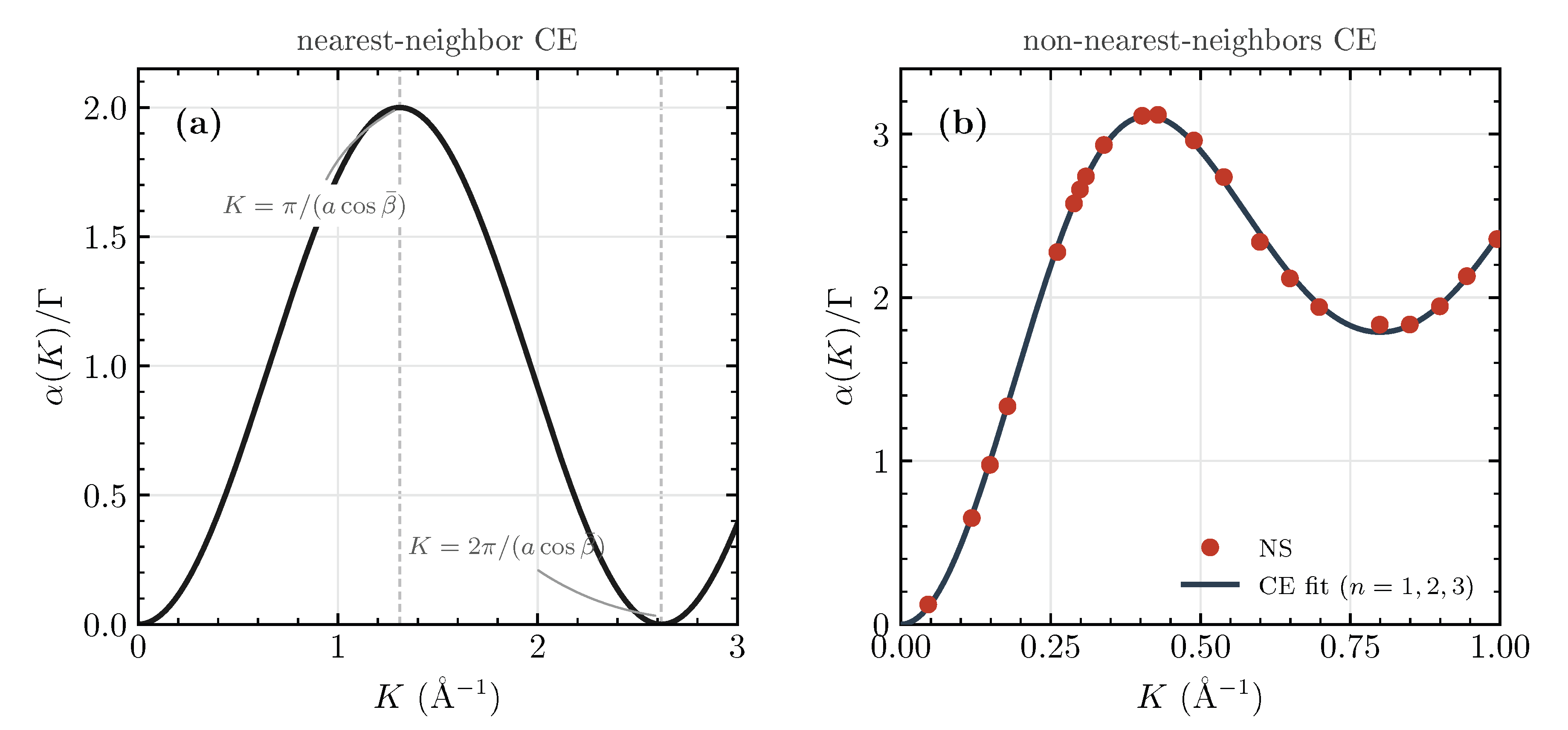
Figure 2 makes the distinction between the nearest-neighbor CE result and its non-nearest-neighbor generalization quantitative. Panel (a) uses the H/Pt(111) observation geometry discussed above ( Å, ) and shows for the nearest-neighbor CE case, Equation (56): a periodic function with a maximum at Å−1 and a node at Å−1, consistent with the vanishing dephasing rate noted above. Since, in the thermally activated regime, the total jumping rate follows an Arrhenius-type law , being a complex function including all the main variables of the diffusion process [21]— deep in the tunneling regime, as for H/Pt(111) at 90 K discussed above, starts flattening and deviates from Arrhenius behavior—only its absolute scale changes with temperature; plotting the dimensionless ratio , as in panel (a), divides this temperature dependence out; the curve shown is therefore the same at any temperature, with T entering only through the overall rate that sets the absolute (not relative) dephasing rate. Panel (b) shows a concrete non-nearest-neighbor realization fitted to numerical-simulation data for Xe diffusion on Pt(111) at 105 K. The points (labelled NS) are dephasing rates obtained from stochastic-wave-function (SWF) simulations [17,18] for a system with lattice spacing Å (with , so that K is measured directly along the jump direction [100]), and the solid line is a least-squares Chudley-Elliott fit including jumps to first, second, and third neighbors (), with the fractional partial rates (), the non-nearest-neighbor form of Equation (56). It is worth noting that this is fewer neighbors than the range reported in [17] to reproduce the full SWF-simulated dynamics for this system: reproducing the complete time-dependent trajectories evidently requires the longer-range tail, whereas the K-dependence of alone—the quantity fitted here—is already well captured by the three leading partial rates, with found to be statistically indistinguishable from zero in the least-squares fit. The fit reproduces the data essentially within symbol size, and the extracted partial jump rates are strongly non-monotonic in n: , i.e., the second-neighbor jump dominates over the first-neighbor one. It is precisely this dominance of a longer jump that produces the characteristic double-lobed K-dependence of —with a secondary maximum beyond the first—which a purely nearest-neighbor model (, a single lobe) cannot reproduce. This illustrates, on real data, the point made in Section 2.4: the exponential lineshape of the ISF is generic, while the specific K-dependence of —and, in particular, how many lobes it develops and where they fall—is fixed entirely by the single-jump distribution entering , i.e., by the lattice and jump mechanism actually realized.
When surface coverage is taken into account, the final expressions for the collective diffusion coefficient and the after-effect function generalize straightforwardly by replacing , again through Equation (52) rather than through any additional lattice-specific assumption.
4. Conclusions
We have shown that the intermediate scattering function, viewed as a characteristic function, organizes the entire hierarchy of linear response functions relevant to helium-scattering studies of surface diffusion—the after-effect function, the generalized susceptibility, the relaxation function and the Green function—and that the time exponential function observed in the diffusive regime follows from the general compound-Poisson (CTRW) structure of the jump process [10,11] rather than from the specific lattice assumptions of the Pauli master equation or the Chudley-Elliott model, which are recovered here as the particular Bravais-lattice case. This formalism should also be extended to any surface diffusion analyzed by other sampling particles- such as photons and neutrons- as long as the Born approximation is valid.
There are very few theoretical works addressing surface diffusion at finite surface coverage, . At very low coverage, adsorbate-adsorbate interactions can be safely neglected, and one speaks of the tracer diffusion coefficient. At higher coverage, however, this interaction can no longer be dismissed, and one speaks instead of the collective diffusion coefficient. Here we have proposed to treat surface coverage as a parameter of the theory, controlled by the experiment, expressing the main functions of the diffusive regime as , , and [23].
The ISA model, as formulated here, is expected to hold for moderate coverages, roughly in the range –. Its main limitation is structural rather than merely quantitative: the model treats adsorbate-adsorbate collisions as a purely statistical, Poissonian shot-noise process, characterized only through the collisional friction of Equation (48), in analogy with an Enskog-type description of uncorrelated hard-sphere collisions. This construction discards, by design, any explicit dependence on the shape and range of the adsorbate-adsorbate interaction potential (attractive or repulsive), on the impact parameter of individual collisions, and on any spatial correlations or short-range ordering that may develop among adsorbates as increases. At low-to-moderate coverage, where collisions are effectively binary and uncorrelated, this simplification is justified and the two-noise-source picture reproduces the observed quasi-elastic lineshape broadening well. The simple analysis proposed to characterize the nature of the adsorbate-adsorbate interaction should be valuable for an initial guess of how this interaction looks like.
Beyond , however, multi-body correlations and incipient ordering are expected to become significant, and a purely collisional friction is unlikely to capture the resulting dynamics; the ISA model should therefore not be extrapolated uncritically to higher coverages without independent verification (e.g., against Langevin simulations with an explicit interaction potential, or against coverage-dependent experimental data) that its two-noise-source assumption remains adequate in that regime.
Finally, a further complementary direction concerns non-Bravais and disordered single-jump distributions in Equation (47)—e.g. reflecting step edges, defects, or amorphous substrates—which, unlike the periodic CE case, would give rise to a non-oscillatory, possibly monotonic ; whether such cases remain within reach of the same CF machinery or not is left for future work.
Author Contributions
Authors have equally contributed.
Funding
Authors acknowledge support of a grant from the Ministry of Science, Innovation and Universities (Spain) with Ref. PID2023-149406NB-I00
Data Availability Statement
Data are available upon request to the authors.
Conflicts of Interest
The authors declare no conflicts of interest.
References
- Van Hove, L. Correlations in space and time and Born approximation scattering in systems of interacting particles. Phys. Rev. 1954, 95, 249–262.
- Vineyard, G. H. Scattering of slow neutrons by a liquid. Phys. Rev. 1958, 110, 999–1010.
- De Gennes, P. G. Liquid dynamics and inelastic scattering of neutrons. Physica 1959, 25, 825–839.
- Lovesey, S. W. Theory of Neutron Scattering from Condensed Matter, Vol. 1: Nuclear Scattering; Clarendon Press: Oxford, UK, 1984.
- Boon, J. P.; Yip, S. Molecular Hydrodynamics; Courier Corporation, 1991.
- Kubo, R.; Toda, M.; Hashitsume, N. Statistical Physics II: Nonequilibrium Statistical Mechanics, Vol. 13; Springer: Berlin, Germany, 2012.
- Hansen, J. P.; McDonald, I. R. Theory of Simple Liquids: With Applications to Soft Matter, 4th ed.; Academic Press, 2013.
- Calvo-Almazán, I.; Fouquet, P. The application of quasi-elastic neutron scattering techniques (QENS) in surface diffusion studies. Eur. Phys. J. Spec. Top. 2012, 213, 149–163.
- Jardine, A. P.; Alexandrowicz, G.; Hedgeland, H.; Allison, W.; Ellis, J. Studying the microscopic nature of diffusion with helium-3 spin-echo. Phys. Chem. Chem. Phys. 2009, 11, 3355–3374.
- Montroll, E. W.; Weiss, G. H. Random walks on lattices. II. J. Math. Phys. 1965, 6, 167–181.
- Weiss, G. H. Aspects and Applications of the Random Walk; North-Holland: Amsterdam, 1994.
- Metzler, R.; Klafter, J. The random walk’s guide to anomalous diffusion: a fractional dynamics approach. Phys. Rep. 2000, 339, 1–77.
- Ala-Nissila, T.; Ferrando, R.; Ying, S. C. Collective and single particle diffusion on surfaces. Adv. Phys. 2002, 51, 949–1078.
- Martínez-Casado, R.; Vega, J. L.; Sanz, A. S.; Miret-Artés, S. Line shape broadening in surface diffusion of interacting adsorbates with quasielastic He atom scattering. Phys. Rev. Lett. 2007, 98, 216102.
- Martínez-Casado, R.; Vega, J. L.; Sanz, A. S.; Miret-Artés, S. Surface diffusion and low vibrational motion with interacting adsorbates: a shot noise description. Phys. Rev. E 2007, 75, 051128.
- Martínez-Casado, R.; Vega, J. L.; Sanz, A. S.; Miret-Artés, S. Stochastic theory for lineshape broadening in quasielastic He atom scattering with interacting adsorbates. Phys. Rev. B 2008, 77, 115414.
- Torres-Miyares, E. E.; Rojas-Lorenzo, G.; Rubayo-Soneira, J.; Miret-Artés, S. Surface diffusion within the Caldeira–Leggett formalism. Phys. Chem. Chem. Phys. 2022, 24, 15871–15890.
- Torres-Miyares, E. E.; Ward, D. J.; Rojas-Lorenzo, G.; Rubayo-Soneira, J.; Allison, W.; Miret-Artés, S. The stochastic wave function method for diffusion of alkali atoms on metallic surfaces. Phys. Chem. Chem. Phys. 2023, 25, 6225–6231.
- Caldeira, A. O.; Leggett, A. J. Path integral approach to quantum Brownian motion. Physica A 1983, 121, 587–616.
- Lindblad, G. On the generators of quantum dynamical semigroups. Commun. Math. Phys. 1976, 48, 119–130.
- Torres-Miyares, E. E.; Miret-Artés, S. Incoherent tunneling surface diffusion. Phys. Chem. Chem. Phys. 2025, 27, 14739–14743.
- Torres-Miyares, E. E.; Miret-Artés, S. The characteristic function method in surface diffusion. Phys. Chem. Chem. Phys. 2026, 28, 8916.
- Torres-Miyares, E. E.; Miret-Artés, S. Surface diffusion at finite coverage: the characteristic function method. Surfaces 2026, 9, 32.
- Papoulis, A. Probability and Statistics; Prentice-Hall, 1990.
- Ushakov, N. G. Selected Topics in Characteristic Functions, Vol. 4; VSP, 1999.
- Torres-Miyares, E. E.; Miret-Artés, S. The quantum-to-classical transition and the H-theorem in surface diffusion. Eur. Phys. J. Plus 2026, 141, 723.
- Haag, G. Modelling with the Master Equation; Springer International Publishing, 2017.
- Breuer, H. P.; Petruccione, F. The Theory of Open Quantum Systems; Oxford University Press, 2002.
- Frenken, J. W. M.; Hinch, B. J. Quasielastic helium scattering studies of adatom diffusion on surfaces. In Helium Atom Scattering from Surfaces; Springer: Berlin, Heidelberg, 1992; pp. 287–313.
- Sears, V. F. High-energy neutron scattering from liquid He4. Phys. Rev. 1969, 185, 200–206.
- Chudley, C. T.; Elliott, R. J. Neutron scattering from a liquid on a jump diffusion model. Proc. Phys. Soc. 1961, 77, 353–361.
- Jardine, A. P.; Lee, E. Y. M.; Ward, D. J.; Alexandrowicz, G.; Hedgeland, H.; Allison, W.; Ellis, J.; Pollak, E. Determination of the quantum contribution to the activated motion of hydrogen on a metal surface: H/Pt(111). Phys. Rev. Lett. 2010, 105, 136101.
Figure 1.
Schematic organization of the linear response functions around the intermediate scattering function , exploiting its role as a characteristic function (CF) of the adsorbate-displacement distribution. Every edge represents a linear, invertible operation (Fourier transform, multiplication by the detailed-balance factor , or time integration/differentiation). Single-headed arrows point from the function(s) on the right-hand side of the cited equation to the one it determines on the left-hand side — e.g., determines via the algebraic inversion of Equation (10), and determines via Equation (24) (the inverse Fourier transform of Equation (7))—though every relation shown is linear and invertible, so it can equally be read in reverse using the same cited equation. The two double-headed arrows mark genuinely symmetric pairs: and , related by the Fourier-transform pair of Equation (2)—and, moreover, the two response functions directly accessible experimentally, by HAS and HeSE, respectively — and and , related by Equation (6) (a time integral one way, a time derivative the other). Equation numbers refer to the derivations in Section 2.1, Section 2.2 and Section 2.3. denotes the dissipative part of , i.e. its imaginary component—itself a real, odd function of — as defined in Equation (10).
Figure 1.
Schematic organization of the linear response functions around the intermediate scattering function , exploiting its role as a characteristic function (CF) of the adsorbate-displacement distribution. Every edge represents a linear, invertible operation (Fourier transform, multiplication by the detailed-balance factor , or time integration/differentiation). Single-headed arrows point from the function(s) on the right-hand side of the cited equation to the one it determines on the left-hand side — e.g., determines via the algebraic inversion of Equation (10), and determines via Equation (24) (the inverse Fourier transform of Equation (7))—though every relation shown is linear and invertible, so it can equally be read in reverse using the same cited equation. The two double-headed arrows mark genuinely symmetric pairs: and , related by the Fourier-transform pair of Equation (2)—and, moreover, the two response functions directly accessible experimentally, by HAS and HeSE, respectively — and and , related by Equation (6) (a time integral one way, a time derivative the other). Equation numbers refer to the derivations in Section 2.1, Section 2.2 and Section 2.3. denotes the dissipative part of , i.e. its imaginary component—itself a real, odd function of — as defined in Equation (10).
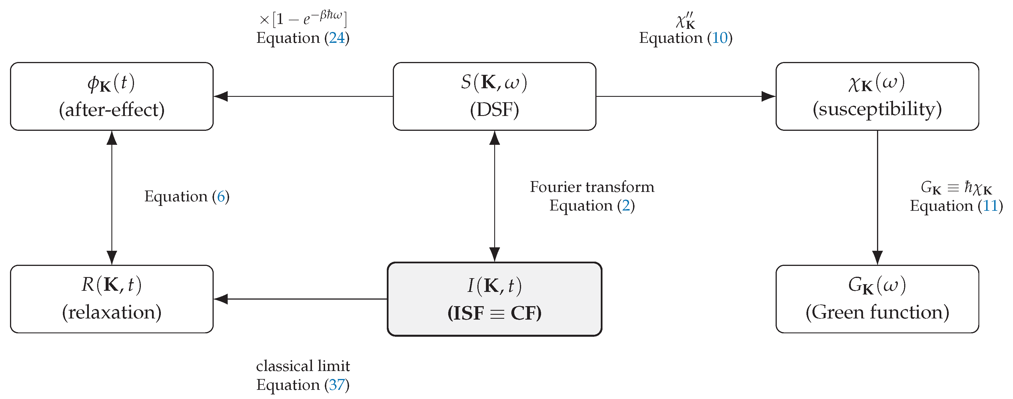
Figure 2.
Dephasing rate , Equations (56) and (47). (a) Nearest-neighbor Chudley-Elliott result for the H/Pt(111) geometry ( Å, ), over Å−1, with both its maximum, at , and its periodic node, at , marked explicitly. (b) Non-nearest-neighbor case fitted to numerical-simulation data for Xe diffusion on Pt(111) at 105 K: points (NS) are dephasing rates from stochastic-wave-function (SWF) simulations [17,18] for a lattice with Å and ; the solid line is a least-squares Chudley-Elliott fit, Equation (47), including jumps to first, second, and third neighbors (), with partial-rate weights . The dominance of the second-neighbor jump () produces the double-lobed K-dependence, which a nearest-neighbor-only model () cannot reproduce. Both panels share the same dimensionless vertical scale but independent axis ranges.
Figure 2.
Dephasing rate , Equations (56) and (47). (a) Nearest-neighbor Chudley-Elliott result for the H/Pt(111) geometry ( Å, ), over Å−1, with both its maximum, at , and its periodic node, at , marked explicitly. (b) Non-nearest-neighbor case fitted to numerical-simulation data for Xe diffusion on Pt(111) at 105 K: points (NS) are dephasing rates from stochastic-wave-function (SWF) simulations [17,18] for a lattice with Å and ; the solid line is a least-squares Chudley-Elliott fit, Equation (47), including jumps to first, second, and third neighbors (), with partial-rate weights . The dominance of the second-neighbor jump () produces the double-lobed K-dependence, which a nearest-neighbor-only model () cannot reproduce. Both panels share the same dimensionless vertical scale but independent axis ranges.
Disclaimer/Publisher’s Note: The statements, opinions and data contained in all publications are solely those of the individual author(s) and contributor(s) and not of MDPI and/or the editor(s). MDPI and/or the editor(s) disclaim responsibility for any injury to people or property resulting from any ideas, methods, instructions or products referred to in the content. |
© 2026 by the authors. Licensee MDPI, Basel, Switzerland. This article is an open access article distributed under the terms and conditions of the Creative Commons Attribution (CC BY) license (http://creativecommons.org/licenses/by/4.0/).
Copyright: This open access article is published under a Creative Commons CC BY 4.0 license, which permit the free download, distribution, and reuse, provided that the author and preprint are cited in any reuse.


