
Submitted:
11 July 2026
Posted:
13 July 2026
You are already at the latest version
Abstract
The Zeta-Minimizer Theorem (ZMT) furnishes a rigorous axiomatic foundation for thermodynamics through three principles—strict concave entropy maximization, uniform Gibbs free energy landscapes with spectral minima, and irreducibility enforced by perpetual bounded oscillations—augmented by helical geometry in which prime numbers emerge as indivisible cycle lengths. The multi-component grand-partition function Z(s) is constructed and establish its universal categorical invariance under functorial mappings, thereby providing a parameter-free backbone for equilibrium and dynamical phenomena. From this structure the thermodynamic conjugate pairs and variational Maxwell relations, the emergence of chemical equilibrium and the equilibrium constant are deductively derived directly from the grand potential, explicit fugacity coefficients, and a variational reaction-rate law governed by the analytical scalar Hessian of the gas-phase reaction coordinate.
For heterogeneous systems solid–fluid interface continuity conditions, marginal stability criteria via the covariant fugacity Hessian are obtained, and—crucially—the first-principles deductive origin of linear scaling relations and Sabatier volcano plots from closed prime functions, without empirical parameters. A complete methodology is developed for ammonia-synthesis loop analysis and catalyst optimization. Central to this methodology is the vapor–solid (V/S) locus, which incorporates inert effects, promoter-induced shifts in effective black-box constants, and distinct operating regimes of Fe- versus Ru-based catalysts. Numerical integrations and Hessian-based kinetic analyses quantitatively recover industrial third-bed behavior, elucidate the lab–industry gap in recent low-pressure studies, and furnish predictive guidelines for next-generation catalyst and process design. The ZMT framework thereby bridges number-theoretic structure with practical chemical engineering, offering zero-adjustable-parameter predictions for sustainable ammonia production.
Keywords:
Zeta-Minimizer theorem
; variational thermodynamics
; heterogeneous catalysis
; ammonia synthesis
; Sabatier volcano
; categorical invariance
; grand-partition function
; Haber–Bosch process
1. Introduction
Ammonia synthesis remains one of the most consequential chemical processes on the planet, underpinning global food production and emerging as a carbon-free energy vector. Despite more than a century of industrial practice, the Haber–Bosch process continues to operate under severe thermodynamic and kinetic constraints, requiring high pressures, elevated temperatures, and expensive promoted iron or ruthenium catalysts whose design still relies heavily on empirical scaling and trial-and-error optimization. Recent pushes toward low-pressure, modular, and renewable-powered ammonia plants have intensified the need for a truly predictive, first-principles framework capable of guiding both catalyst formulation and reactor design [1,2,3,4,5,6,7,8,9,10,11,12,13,14,15].
Existing theoretical tools—density-functional scaling relations, microkinetic modeling, and Sabatier-type volcano plots—have provided invaluable qualitative guidance yet remain largely inductive or semi-empirical. Linear scaling relations, for example, are typically extracted from large DFT datasets rather than derived from thermodynamic axioms; their transferability across promoters, supports, and operating regimes is limited, and they offer little direct insight into the role of inerts, interface stability, or the coupling between gas-phase kinetics and vapor–solid equilibration. A deductive framework that begins from a small set of thermodynamic axioms and rigorously derives classical thermodynamic relations, equilibrium constants, reaction rates, and the emergence of scaling and volcano behavior would constitute a significant advance.
This work develops a fully deductive, parameter-free framework for heterogeneous catalysis and chemical reaction engineering [16,17], built from three primitive axioms and the helical geometry of the grand-partition function. The manuscript is organized as follows.
Section 2, Section 3 and Section 4 establish the axiomatic and geometric foundations of the Zeta-Minimizer Theorem (ZMT). The three axioms are introduced, the helical operator, and the effective Hessian PDE, followed by the categorical invariance of the grand-partition function and the solid–fluid interface matching condition that yields the interface constants .
Section 5, Section 6 and Section 7 derive the variational emergence of classical thermodynamics and chemical equilibrium [18,19,20,21]. Showing how conjugate pairs, phase equilibria, extent of reaction, and multi-reaction multi-phase equilibrium arise directly from minimization of the phase functional, without empirical assumptions.
Section 8 presents the variational reaction rate law, its linearization near equilibrium, and the emergence of batch and residence time [16,17]. From the same framework deductively recovering linear scaling relations, Sabatier volcano plots, modal decomposition of coupled dynamics, and the classical seven-step heterogeneous catalysis sequence [16,17] as emergent normal modes.
Section 9 applies the complete variational model to industrial ammonia synthesis. The explicit phase functional for the N₂–H₂–NH₃–inert system are constructed, deriving the exact nonlinear driving force and scalar Hessian, obtaining the implicit analytical solution for transient conversion, and quantifying the relative impact of inerts and pressure.
Section 10 demonstrates that the classical Temkin–Pyzhev rate expression [16,17] emerges as a limiting case of the ZMT variational rate law in the high-inerts regime, while the ZMT formulation remains regular and physically consistent at low inerts and low pressure.
Section 11 provides experimental and DFT validation. Interpreting formation energies of adsorbed promoters, N adsorption energies, N–N transition-state barriers, and promoter-induced electric fields through the lens of interface constants and surface gear occupations, and we validate the framework against catalyst activity data obtained at constant pressure and zero inerts.
Section 12 offers a comparative industrial analysis. Contrasting the operating regimes of Fe- and Ru-based catalysts, re-examining recent low-pressure ammonia synthesis studies through the ZMT lens, and discuss the critical role of inerts and the lab–industry gap.
2. ZMT Axiomatic Foundation and Helical Geometry
The Zeta-Minimizer Theorem (ZMT) provides a deductive unification of statistical mechanics, number theory, and helical geometry [22,23,24]. All macroscopic thermodynamics, electromagnetic phenomena, and magnetic transport emerge from three primitive axioms. These axioms uniquely select the non-proper Archimedean conical helix as the background geometry satisfying bounded oscillations, flux conservation, and entropy maximization (Topology Selection Theorem S4 [22]) [23,24].
2.1. The Three Axioms
2.1.1. Axiom 1 (Strict Concave Entropy Maximization)
2.1.2. Axiom 2 (Uniform Gibbs Free Energy with Spectral Minima)
2.1.3. Axiom 3 (Irreducibility via Perpetual Bounded Oscillations)
Primes induce irreducible representations (Hilbert–Maschke theorem) of the helical flux, ensuring divergence-free flow
and trigonometric boundedness (Lemmas S8 and S9 [23,24,25]). The background prime 19 is the fixed upper edge of the stability window.
These axioms uniquely select the non-proper Archimedean conical helix as the background geometry and force primes to act as indivisible bosonic modes with energies (Cycle-to-Prime Mapping, Sub-Lemma S9 [22,23,24]).
In physical terms, these three axioms encode the foundational principles of thermodynamics [23,24,25,26,27,28], gauge theory [29,30], and topology [31] as follows:
Axiom 1 (Strict Concave Entropy Maximization) is the variational statement of the Second Law: entropy is strictly concave, guaranteeing a unique global thermodynamic equilibrium and a single minimum of the grand potential [23,24,25,26,27,28].
Axiom 2 (Uniform Gibbs Free Energy with Spectral Minima) enforces equality of the molar Gibbs free energy across coexisting phases through a strict positive spectral gap in the helical operator — the molar analogue of the Einstein photoelectric threshold [31], ensuring no zero-energy excitations are allowed.
Axiom 3 (Irreducibility via Perpetual Bounded Oscillations) combines Noether’s theorem (exact conservation of helical flux) with topological irreducibility of modes. This forbids zero-helicity states and ensures perpetual bounded oscillations, realizing microscopically the QED prohibition of longitudinal photons [32,33] through the irreducible prime-length rotational symmetries of the helix.
Taken together, the axioms generate a grand potential whose functional form deductively encodes the forbidden zero-helicity sector [23,24]. The grand-partition function (Section 3.2) therefore emerges as the universal generator of the entire theorem — the categorical crown jewel that converts the three axioms into concrete, zero-parameter predictions across thermodynamics, electromagnetism, and superconductivity [22,23,24].
2.2. Prime Numbers as Indivisible Cycle Lengths
A prime corresponds to an irreducible -fold rotational symmetry that cannot be decomposed into smaller closed cycles. This follows directly from Axiom 3: the helical operator must act on a minimal, indivisible representation whose dimension/order is exactly (Lemma S8 [22,24]).
The angular quantization step encoded in every helical projection is
2.3. Explicit Helical Operator and Effective Hessian PDE
2.3.1. ZMT Helical Operator
Axiom 2 requires a self-adjoint elliptic operator whose Gibbs functional
has a strict positive spectral gap (Lemma S4 [22,23,24]). The unique operator satisfying these conditions is the Sturm–Liouville form
where the centrifugal term encodes the conical taper and is fixed by the helicity constraint of Axiom 3. The Friedrichs extension ensures self-adjointness, and elliptic regularity plus the non-proper condition guarantee (Corollary S1 [22,24]).
2.3.2. Effective Hessian PDE
Combining the entropy functional (Axiom 1) and the Gibbs functional (Axiom 2) yields the phase functional
where is the constant curvature floor enforced by Axiom 3 (Lemma S11 [22,23,24]).
Direct Euler–Lagrange variation with respect to produces the stationarity condition
or explicitly
Here the source term is
with the entropy density, the second covariant derivative along the helix, and the Lie derivative along the helical tangent vector. This effective Hessian PDE is a true theorem of ZMT (Corollary S1 [22,23,24]), derived solely from the three axioms and the explicit helical operator.
3. Variational Thermodynamics of Multi-Component Helical Systems and Categorical Invariance of
The Riemann Hypothesis is reinterpreted in the ZMT framework as a thermodynamic stability condition [22,23,24]: the equilibrium frequency spectrum (Lyapunov exponents) is minimized only when the thermodynamic parameter satisfies (strict concavity of the Gibbs functional from Axiom 1). Any deviation off the line would violate the spectral gap (Axiom 2) or the divergence-free flux condition (Axiom 3). Thus, the physical grand-partition function must be constructed so that its dominant component always occupies more than half the total occupation when equilibrium is reached on the critical line (Theorem S26 [22,24]).
3.1. Grand-Partition Function (General Multi-Component Case)
The grand-partition function for an arbitrary multi-component system is constructed once from the helical gears present in the mixture [23,25]:
where is the deductive molecular (or elemental) prime of component , and the product runs over all gears (each with multiplicity exactly 1) (Helical Gear Multiplicity Theorem S33 [22,24]).
3.2. Mole Fractions (General Multi-Component Case)
The global mole fraction of gear is therefore
3.3. Lyapunov Exponent per Gear
3.4. Interaction Parameter per Gear
The interaction parameter for each gear satisfies the linear first-order ODE that enforces the global minimum of the mixture frequency at the critical composition [22,23,24]:
where the integration constant is fixed by the critical-point condition (Section 4.2).
3.5. Critical Composition per Gear () in the Limit
3.6. Rigorous Physical Interpretation of Integer Gear-Up-to-Prime Rule
Under the integer gear-up-to-prime rule (Helical Gear Multiplicity Theorem S33 [22,24]), each component with deductive prime occupies exactly the gears (each with multiplicity 1). This rule follows directly from Axiom 3: the helical operator must act on a minimal, indivisible representation whose dimension/order is exactly the prime . Any smaller or larger set would either be reducible (violating irreducibility) or introduce extraneous modes (violating entropy maximization, Axiom 1).
3.6.1. Definition of a Gear
A gear is a discrete, indivisible helical winding mode labeled by an integer . Mathematically, each gear corresponds to an irreducible representation of the helical operator (Eq. (3)) with winding angle [22,23,24]
Physically, a gear represents a quantized collective excitation of the helical flux with a fixed angular periodicity. The occupation number of gear is the Bose–Einstein factor (Eq. 10)
which gives the average number of helical quanta in that mode at thermodynamic parameter .
3.6.2. Integer Gear-Up-to-Prime Rule
For any component with deductive prime , the allowed gears are exactly the integers
3.6.3. Integer Gear-Up-to-Prime Rule Axiomatic Deduction
The rule is not postulated; it is the unique outcome of the three axioms acting together on the helical representation graph.
- Axiom 1 (Strict Concavity) demands the smallest possible set of modes that can still achieve a unique global minimum of the phase functional . Including gears beyond would introduce redundant modes, increasing the variational cost without lowering the grand potential.
- Axiom 2 (Spectral Gap) guarantees a positive lower bound on all eigenvalues. The integer sequences up to the prime is the minimal set that satisfies both indivisibility and the spectral gap while allowing the observed stability window around prime 19.
Thus, the rule follows deductively: the helical operator must act on irreducible prime-length cycles (Axiom 3), the phase functional selects the smallest such set (Axiom 1), and the spectral gap is preserved only within that window (Axiom 2).
3.6.4. Physical Interpretation
- Each gear behaves as a quantized tooth on the helical driveshaft.
3.7. Universal Property of in Category Theory
To prove that the grand-partition function satisfies the universal property required of the functorial backbone of the Zeta Minimizer Theorem [22,23,24].
3.7.1. Definition of Categories
Objects are multi-component helical gear systems equipped with the star-topology representation graph [22,23,24] (anchored at prime 19) and integer-gear occupations .
Morphisms are natural transformations [24,37,38] that preserve the star topology [24,39,40], the integer-gear-up-to-prime rule, and the action of the helical operator .
Let be the category whose:
Objects are thermodynamic potentials [27] (real-valued functions of the reduced variable ).
Morphisms are natural transformations between these potentials that commute with differentiation with respect to .
3.7.2. Definition of Functor
Define the functor
by sending each object to the grand-partition function
and each morphism to the induced natural transformation on the potentials [24].
3.7.3. Universal Property Theorem
Theorem 1 [24]. (i.e., the functor ) satisfies the following universal property:
For any other functor that assigns to each helical gear system a thermodynamic potential compatible with the three axioms (strict concavity of the phase functional, positive spectral gap of , and flux conservation), there exists a unique natural isomorphism
such that the diagram (Figure 1) commutes for every morphism in .
Proof of Theorem 1.
- By Axiom 1 the phase functional is strictly concave and possesses a unique global minimizer.
Thus is the canonical (universal) functor from helical gear systems to thermodynamic potentials. This categorical universality guarantees that every derived quantity — Lyapunov exponents, interface matching conditions, conjugate pairs, electromagnetic fields, and superconducting shells — is representation-independent and deductively fixed once and for all by the three axioms.
3.8. Categorical Invariance of the Grand-Partition Function — The Functorial Backbone of ZMT
The grand-partition function is not merely a formal generating function; it is the image of a functor [24,39,40] from the category of helical gear systems (whose objects are multi-component mixtures equipped with the star-topology representation graph anchored at prime 19, and whose morphisms are natural transformations that preserve the integer-gear-up-to-prime rule) into the category of thermodynamic potentials [24,37,38,40,42]. This functorial invariance guarantees that every derived quantity — mole fractions , Lyapunov exponents , interaction parameters , critical compositions, interface matching conditions, and thermodynamic conjugate pairs — is canonically defined and independent of arbitrary choices of basis or labeling. Without this categorical foundation, the three primitive ZMT axioms would be insufficient to produce a unique, consistent thermodynamic mapping. The universal invariance of is therefore the indispensable glue that elevates the axioms and helical geometry into a rigorous, representation-independent framework for all subsequent results.
3.8.1. Functorial Isomorphism Theorem Statement
Theorem 2 [24]. Let be any flux-like density satisfying Axiom 3 (irreducible bounded oscillations + divergence-free flux conservation [22,23,24]) and let be its thermodynamically conjugate extent variable (i.e., the variable appearing with opposite sign in the differential of the Gibbs free energy) [43,44]. The phase functional (identified with the Gibbs free energy ) is strictly concave (Axiom 1). Therefore, the Legendre transform structure with respect to at fixed temperature (fixed ) yields the exact relation
for any such conjugate pair . This is the Functorial Isomorphism Theorem (Theorem S28 [22,24]).
Proof of Theorem 2. The gear occupations that define are determined solely by the helical operator and the star-topology representation graph (Topology Selection Theorem S4 [22,23,24]). Because gear discretization commutes with all scaling transformations and because Axiom 3 forces the flux density to appear linearly in the source tensor , the product factors out of the phase functional exactly as , independent of the specific physical identity of .
3.8.2. Explicit Examples of the Universal Isomorphism
Because is the same grand-partition function in every case, the isomorphism (Eq. (17)) holds uniformly [24,27,41,45]:
- Mechanical pair (pressure–volume):
- Magnetic pair (field strength–magnetization):
- Electric pair (field strength–polarization):
- Electrochemical pair (potential–charge density):
All four (and any future) conjugate pairs are governed by the identical functional [24].
3.8.3. Strict Validity of the Functorial Mapping of
The grand-partition function is not a physical observable tied to any particular variable. It is the universal functor [24,42,45] that maps the helical mode occupations of any multi-component system to the complete set of thermodynamic observables [24,35,36,38,39,42].
The phase functional remains the single variational generator (Axiom 1 of the Zeta Minimizer Theorem). The helical operator and the representation graph are fixed uniquely and globally by the three axioms together with the Topology Selection Theorem (Theorem S4 [22,23,24]).
Consequently, is an intrinsic property of the helical gearbox itself, independent of which flux density or conjugate variable is chosen for measurement. Different physical realizations (pressure, magnetic field, electric field, electrochemical potential, etc.) are merely distinct projections of the same underlying helical modes. The functorial isomorphism therefore guarantees that all projections share the identical, representation-independent currency .
This categorical structure eliminates any possibility of category mismatch and ensures that every subsequent derivation — from Lyapunov exponents and interface matching to electromagnetic fields and superconducting shells — is canonically defined and internally consistent.
3.8.4. Experimental Anchor and Zero-Parameter Predictive Power
The universal grand-partition function is anchored to the pure prime-19 background sea. High-precision compressibility measurements confirm that the identical reproduces the experimental equation-of-state residuals to sub- accuracy [23].
Because the same governs every thermodynamic conjugate pair, the Zeta Minimizer Theorem automatically yields zero-parameter predictions for magnetic susceptibility [46,47], electric polarization [48,49], electrochemical potentials [50,51,52], and superconducting critical fields [53,54]. Pressure–volume relations, magnetic response, electric response, and electrochemical behavior are therefore revealed as distinct projections of the identical underlying helical modes.
4. Solid–Fluid Interface Matching and Marginal Stability
The interface between solid and fluid phases is the critical location where the variational principles of the Zeta-Minimizer Theorem (ZMT) enforce thermodynamic and mechanical consistency. All derivations follow directly from the phase functional , the grand-partition function , and the three primitive axioms.
4.1. Grand-Potential Continuity Condition
At equilibrium the total Gibbs free energy (identified with the phase functional by Axiom 1) must be minimized globally. For two coexisting phases (solid and fluid) in contact, the grand potential must be continuous across the interface up to a fixed per-gear constant determined by marginal stability [27,28,55].
Define the grand-potential difference between the solid and fluid phases as
Thermodynamic equilibrium requires that any infinitesimal variation of the interface position leaves the total grand potential unchanged:
Because the grand-partition function has the same functional form in both phases (Eq. (9)), the only variational freedom at the boundary is the redistribution of gear occupations . The stationarity condition is therefore
where each constant is fixed once by the critical composition of gear (Interface Matching Theorem S45 [22,24]). This is the grand-potential continuity condition at the solid–fluid interface.
4.2. Derivation of Integration Constants
The constants are obtained by enforcing the global minimum of the mixture frequency at the critical composition in the limit.
From the grand-partition function (Eq. (9)), the occupation of gear is given by Eq. (10):
In the limit ,
The total occupation behaves as
The critical mole fraction of gear is therefore (Eq. (14))
The interaction parameter for gear satisfies the linear first-order ODE (Eq. (13)) that enforces the global minimum of the mixture frequency at :
Integrating this ODE and imposing the critical-point condition at yields the exact deductive expression
4.3. Marginal Stability at the Interface
The system reaches marginal stability when the least negative Lyapunov exponent among all gears reaches zero:
Substituting the interaction parameter (Eq. (13)) into the Lyapunov exponent formula (Eq. (12)) gives
At the solid–fluid interface the lowest gear () dominates because it has the strongest geometric leverage. Setting enforces the marginal-stability condition that defines the superconducting or phase-transition shell at the boundary.
4.4. Role of the Covariant Fugacity Hessian
The continuity condition (Eq. (26)) is enforced by the stationarity of the phase functional . The covariant fugacity Hessian (Corollary S1 [22,23,24]) projected onto the interface normal yields the effective boundary condition
where is the source term (Eq. (8)). This equation, together with the grand-potential continuity (Eq. (22)), guarantees that both thermodynamic continuity and mechanical/electromagnetic consistency are satisfied simultaneously across the solid–fluid boundary.
5. Thermodynamic Conjugate Pairs and Variational Maxwell Relations
In the Zeta-Minimizer Theorem, all thermodynamic quantities arise as functorial shadows of the global minimization of the phase functional on the non-proper Archimedean conical helix (Topology Selection Theorem S4). This structure naturally generalizes the classical pressure–volume conjugate pair to arbitrary thermodynamic conjugate pairs.
5.1. General Conjugates
Let be any flux-like density satisfying Axiom 3 (divergence-free flux conservation) and let be its thermodynamically conjugate extent variable. The phase functional is strictly concave (Axiom 1), so the Gibbs free energy admits a Legendre transform at fixed temperature (fixed ) [23,24]:
Because gear discretization commutes with scaling transformations, the product of any conjugate pair satisfies the natural isomorphism by Eq. (17)
5.2. Classic Pressure–Volume Conjugate Pair
The general structure maps directly to the familiar conjugate pair , where is pressure (independent variable) and is molar volume (dependent variable) [22,24]. The entropy is
The thermodynamic differential of the Gibbs free energy reads
5.3. Clapeyron Equation (Equilibrium Slope)
Along an equilibrium line at the global minimum of () the two differentials must balance:
Solving for the slope of the coexistence curve gives the classic Clapeyron equation:
Substituting the ZMT expressions for and yields the explicit form in terms of the grand-partition function:
This relation is fully deductive: it follows directly from the stationarity condition of the phase functional (Axiom 1) and the conjugate-pair isomorphism (Eq. (17)).
5.4. Variational Maxwell Relations
The covariant fugacity Hessian is symmetric by construction (self-adjoint helical operator from Axiom 2). Therefore, the mixed second derivatives of the phase functional commute, and the thermodynamic potentials satisfy the variational Maxwell relations [22,24]:
for any conjugate pair . These relations hold for magnetic, electric, and all other pairs (Variational Maxwell Relations Theorem S37 [22,24]).
All results in this section follow deductively from the three axioms of the Zeta-Minimizer Theorem and the functorial invariance of with no additional postulates.
5.5. Thermodynamic Potentials and Heat Capacities
All thermodynamic potentials and heat capacities are generated from the same grand-partition function and therefore share identical functional forms for both magnetic and electric conjugate pairs [24,47,56,57]. The explicit expressions (derived consistently from the entropy (Eq. (30)) and the Gibbs free energy ) are collected in Table 2.
6. Variational Emergence of Classical Phase Equilibria in Non-Reactive Multi-Component Systems
6.1. Phase Functional Extensivity in Non-Reactive Multi-Component Systems Theorem
Theorem 3. In the ZMT framework, the phase functional of a non-reactive multi-component system satisfies exact extensivity:
Molar (intensive) phase functional
Total (extensive) phase functional
where and the molar grand-partition function is
with the macroscopic mole fraction of component in the mixture.
Definitions
- : molar Gibbs free energy of the mixture (per mole).
- : total Gibbs free energy of the macroscopic phase.
- : molar grand-partition function of the phase.
- : contribution from the helical gears exclusive to component .
- : contribution from the prime-19 master hub (background vacuum).
- Non-reactive: mole numbers are independent (no stoichiometric constraint).
Proof of Theorem 3.
- Gear assignment: By Axiom 3 and the integer gear-up-to-prime rule, each species is assigned a unique prime identifier and a fixed, indivisible set of helical gears with contribution .
- Occupational independence: In the absence of chemical reaction, the gears of different species are occupationally independent.
- Star-topology product structure: The prime-19 star topology (master hub + independent spokes) implies that the grand-partition function of the mixture factors as
-
Molar normalization: Normalizing to one mole of mixture and expressing each species contribution per mole via its mole fraction yieldsPhase-functional identification: By the foundational ZMT map, the molar phase functional (Eq. (36)) is
- Extensivity: For a macroscopic system of moles, the total phase functional scales linearly (Eq. (37)):
This completes the proof. Every step follows directly from the helical gear construction, star topology, and species independence in the non-reactive limit. □
Corollary 1. The phase functional is homogeneous of degree 1 in the particle numbers, satisfying the fundamental requirement for a consistent thermodynamic potential in extensive systems.
6.2. Emergence of Chemical Potential from the Phase Functional Theorem
Theorem 4. In a non-reactive multi-component phase [18,19,20,21] within the Zeta-Minimizer framework, the chemical potential of component is obtained exactly from the total phase functional as
where is the species-specific correction arising from the gas–solid interface matching constants .
Definitions
- : total (extensive) phase functional of the system.
- : molar phase functional.
- : macroscopic mole fraction of component in the mixture.
- : contribution to the grand-partition function from the helical gears of component .
- : deductive shift originating from the interface matching constants of component (enforced by grand-potential continuity).
Proof of Theorem 4.
- 1.
- Total phase functional: From Theorem 3 (Eq. (37)),
- 2.
-
Definition of chemical potentialDifferentiating at constant gives , so
- 3.
- Derivative of the molar functional: Since (Eq. (36)),
- 4.
- Explicit dependence of on : From the product structure (Eq. (38))taking the logarithmic derivative at constant (only changes) and using together with the normalization , the cross terms cancel exactly, yielding
- 5.
- Final assembly: Substituting back and collecting terms giveswhere the interface correction enters directly from grand-potential continuity at the solid–fluid boundary (Section 4).
This completes the proof. All steps follow strictly from extensivity (Theorem 3), the product structure of , and interface matching.
Corollary 2. The factor supplies the exact analogue of the classical fugacity coefficient , while the constants provide the deductive counterpart of the reference-state chemical-potential shift [18,19,20,21]. Thus both the activity coefficient and the standard-state correction [18,19,20,21] emerge naturally and parameter-free from the ZMT construction.
6.3. Vapor-Liquid Equilibrium and Classical Fugacity/Activity Coefficients Emergence Theorem
Theorem 5. In the Zeta-Minimizer framework, vapor-liquid equilibrium (VLE) emerges as the equality of chemical potentials between coexisting phases [18,19,20,21]. The helical fugacity factor and the interface matching constants recover the classical fugacity coefficient and activity coefficient (including the reference-state correction) without additional postulates.
At equilibrium between a vapor phase (V) and a liquid phase (L), the chemical potential of every component is equal:
This equality is equivalent to the classical fugacity relation [18,19,20,21]
where is the vapor-phase fugacity coefficient, and both and the reference fugacity arise from the difference in phase-specific helical gear structures and the interface constants .
Proof of Theorem 5.
- Chemical potential in any phase: From Theorem 4, the chemical potential of component in a given phase (Eq. (40)) iswhere is the molar phase functional of that phase, is the helical-gear contribution of species in that phase, and is the interface correction.
- Equilibrium condition: At VLE the total phase functional of the combined system is stationary with respect to matter transfer between phases. Hence
- Substitution: Inserting the expression from Step 1 for both phases (using for the vapor mole fraction and for the liquid) yields
- Rearrangement: Collecting terms gives
- Identification of classical coefficients: The left-hand side contains the composition and helical fugacity factors. Identifying . The right-hand side is the difference in molar phase functionals plus the difference in interface corrections, which is exactly Exponentiating and multiplying through by recovers the classical VLE condition [18,19,20,21]
Corollary 3. The helical factor is the direct deductive analogue of the fugacity coefficient . The phase-specific gear structures together with the interface matching constants supply the origin of the activity coefficient and the reference fugacity . Classical VLE thermodynamics [18,19,20,21] is therefore an emergent consequence of variational optimization on the helical manifold.
6.4. General Multi-Phase Multi-Component Equilibrium Emergence Theorem
Theorem 6. In the Zeta-Minimizer framework, thermodynamic equilibrium [18,19,20,21] in a system of phases and components (non-reactive or reactive) is completely characterized by the equality of the chemical potential of each component across all phases:
This single condition recovers all classical equilibrium criteria (VLE, LLE, SLE, VLLE, and chemical-reaction equilibrium).
Definitions
- : molar phase functional of phase .
- : total extensive phase functional of the multi-phase system.
- : chemical potential of component in phase .
- : helical-gear contribution of component in phase .
- : interface matching constants of component in phase .
- : number of coexisting phases.
- : number of components.
Proof of Theorem 6.
- Phase functional per phase: By Theorem 3, each phase possesses its own molar phase functionalwhere is constructed from the helical gears present in that phase.
- Chemical potential per phase: From Theorem 4, the chemical potential of component in phase is
- Global stationarity: Equilibrium minimizes the total phase functional . Any virtual transfer of component between phases must satisfy , which requiresand for every component
- Equality across all phases: Extending the pairwise condition to the full set of phases gives
-
Recovery of classical conditions: Substitution of the expression from Step 2 into the equality and rearrangement directly yields:
- For phase equilibria (VLE, LLE, SLE, …): , where and , originate from differences in and between phases.
- For chemical reactions: the same -equality combined with the stoichiometry matrix produces the equilibrium constant
Corollary 4. The helical factor is the direct origin of the classical fugacity coefficient in phase [18,19,20,21]. Differences in gear occupation and interface constants across phases generate the activity coefficient and the reference fugacity .
7. Variational Emergence of Chemical Equilibrium in Reactive Systems
7.1. Extent of Reaction as a Variational Parameter
An independent chemical reaction is written in the standard form [18,19,20,21]
where for reactants and for products.
The extent of reaction parameterizes the instantaneous composition. The mole change of each species is
and the mole fractions become
The grand-partition function of the reacting mixture is therefore a function of through the collective gear occupations.
7.2. Global Minimization of the Phase Functional Determines
By Axiom 1, is strictly concave in . Consequently it possesses a unique global minimizer satisfying
This single stationarity condition simultaneously determines:
- the equilibrium composition at the gas–solid boundary,
- the consumption of each reactant and formation of each product,
- the final gear union
Any species may be chosen as reference; its change fixes , and stoichiometry then determines all other . The global minimization of automatically couples all gear occupations through the star-topology source tensor.
7.3. Extent of Reaction as Natural Constraint in ZMT
The star topology implies that every gear interacts only through the prime-19 anchor. Global minimization of nevertheless imposes a collective constraint across the entire mixture. The scalar is the single variational parameter that re-allocates gears along the atomic shaft while automatically satisfying the interface matching condition (Eq. (24))
at .
7.4. Single-Reaction Summary
For any single independent reaction, the extent may be defined with respect to any participating species. All molar changes are then fixed by the stoichiometric coefficients. This constraint is already encoded in the global minimization of the phase functional and the grand-partition function at the boundary. No additional postulate is required.
7.5. Generalization to Multiple (Coupled) Reactions
7.5.1. Stoichiometry Matrix and Independent Reactions
Consider species and candidate reactions. The stoichiometry matrix (size ) has columns that are the stoichiometric vectors of each reaction. The number of independent reactions is
Any set of linearly independent columns forms a basis for the reaction space.
7.5.2. Extent-Vector Parameterization and Mole-Fraction Evolution
Define the extent vector The change in moles of species is
The gear occupations and grand-partition function then depend on :
Equilibrium occurs at the global minimum of with respect to :
7.5.3. Equilibrium Gas Composition
The equilibrium composition satisfies both the interface matching condition and the stationarity of . Linear dependence among reactions is automatically eliminated by restricting to the independent extents.
7.5.4. General Variational Methodology for Multi-Reaction Systems
- Construct the stoichiometry matrix and compute .
- Parameterize the system by the extent vector .
- Express all gear occupations and the phase functional .
- Solve the system () for .
- Obtain the equilibrium gas composition from and the interface matching condition.
This procedure is fully deductive: multiple reactions are treated as a single global minimization of on the star-topology shaft, with the rank condition ensuring no redundancy. The framework extends directly to biochemical networks and any multi-reaction system.
7.6. Phase Functional Extensivity in Reactive Systems Theorem
Theorem 7. In the Zeta-Minimizer framework, for a reactive multi-component system in which the species mole numbers are linked through independent extents of reaction (), the phase functional satisfies exact extensivity:
- 1.
- Molar (intensive) phase functional (Eq. (36)),
- 2.
- Total (extensive) phase functional (Eq. (37)),
Here is the molar grand-partition function, which depends parametrically on the reaction extents through the stoichiometric constraints on the mole numbers.
Definitions
- : molar phase functional of the reactive mixture.
- : total extensive phase functional of the macroscopic reactive system.
- : extent of the -th independent reaction (variational parameter).
- : mole number of component , constrained by stoichiometry.
- : total number of moles in the phase.
- : molar grand-partition function of the reactive mixture, dependent on and the extents via the mole fractions
Proof of Theorem 7.
- Stoichiometric constraint: By the stoichiometry matrix, the mole numbers are linked:
- Grand-partition function dependence: The grand-partition function is constructed from the helical-gear contributions of all species. Because the macroscopic mole fraction depend on the mole numberswhere the dependence enters exclusively through the mole fractions in the product structure.
- Molar phase functional: By the foundational ZMT identification,
-
Extensivity: For a macroscopic system of moles, the total phase functional scales linearly:The stoichiometric subspace preserves homogeneity of degree 1 in
- Variational consistency: The extents are themselves variational parameters. Minimization of is performed jointly with respect to the overall system size and the reaction coordinates , maintaining full thermodynamic consistency.
Corollary 7. The molar phase functional remains a well-defined state function of , , and the reaction extents
Corollary 8. The chemical potential of component is still given by , with the derivative taken along the allowed stoichiometric subspace defined by the reaction extents.
Corollary 9. This theorem supplies the foundation for the derivation of chemical equilibrium constants and multi-phase reactive equilibria in subsequent results.
7.7. Chemical Potential in Reactive Systems Theorem
Theorem 8. In the Zeta-Minimizer framework, for a reactive multi-component system in which species mole numbers are linked through independent extents of reaction , the chemical potential of each component is rigorously defined as the partial derivative of the total phase functional taken along the stoichiometric subspace.
Statement:
where the derivative respects the stoichiometric constraints, and evaluates to
Here is the molar phase functional of the reactive mixture and the derivative is performed along the allowed stoichiometric subspace.
Definitions
- : total extensive phase functional of the reactive system.
- : molar phase functional of the reactive mixture.
- : macroscopic mole fraction of component in the mixture.
- : vector of independent reaction extents (variational parameters).
- Stoichiometric subspace: the manifold in composition space defined by
Proof of Theorem 8.
- 1.
- Total phase functional: From Theorem 7,with dependence on entering through the mole numbers .
- 2.
- Variational definition: The chemical potential iswhere the derivative is taken along the stoichiometric subspace (i.e., when changes, the other adjust according to the stoichiometry matrix so the variation remains in the allowed reaction manifold).
- Chain rule:
- Derivative of the molar functional: Since , differentiation along the stoichiometric subspace using the product structure of and the definition of mole fractions yields, after cancellation of cross terms,where is the interface matching contribution.
- Consistency: The derivative is confined to the stoichiometric subspace defined by the matrix . This ensures the chemical potential remains well-defined even though the individual are not independent.
Corollary 10. The chemical potential retains the classical form correction, where the activity incorporates the helical fugacity factor and the mole fraction
Corollary 11. The reaction affinity of the -th independent reaction is
which supplies the variational driving force for each reaction.
Corollary 12. When all , the expression reduces exactly to the non-reactive chemical potential of Theorem 4, providing a continuous bridge between the two regimes.
7.8. General Multi-Reaction Multi-Phase Equilibrium Emergence Theorem
Theorem 9. In the Zeta-Minimizer framework, complete thermodynamic equilibrium in a multi-phase, multi-component, multi-reaction system is achieved when two conditions hold simultaneously: (i) the chemical potential of every component is identical in all coexisting phases, and (ii) the affinity of every independent reaction vanishes. Both conditions emerge directly from the minimization of the total phase functional.
Statement:
At equilibrium:
- 1.
- Phase equilibrium
- 2.
- Chemical-reaction equilibrium
These conditions recover the full set of classical equilibrium relations, including multi-phase phase equilibria and the thermodynamic equilibrium constants for simultaneous reactions [18,19,20,21]:
Definitions
- : chemical potential of component in phase .
- : affinity of the -th independent reaction.
- : thermodynamic equilibrium constant of the -th reaction.
- : activity of component (incorporating both composition and the helical fugacity/activity coefficients from ZMT).
Proof of Theorem 9.
- 1.
- Step 1 (Total phase functional) The total phase functional of the entire system is
- 2.
-
Variational stationarity: Equilibrium requires to be stationary with respect to every allowed variation:
- transfer of any component between any phases,
- advancement of any independent reaction extent
- 3.
- Phase equilibrium from matter transfer: A virtual transfer of component from phase to phase produces zero change in only if
Extending to all phases yields the multi-phase chemical-potential equality.
-
Chemical equilibrium from reaction advancement: A virtual advancement of the -th independent reaction producesStationarity requires
-
Recovery of classical constantsSubstituting the expression for from Theorem 8 into yieldswhich rearranges directly to the classical equilibrium constant
Corollary 13. All thermodynamic equilibria — phase, chemical, and their combination in multi-phase reactive systems — are unified under the single principle of minimizing the total phase functional
Corollary 14. The number of independent variables is reduced by (from chemical-potential equalities) plus (from vanishing affinities), recovering the generalized Gibbs phase rule for reactive multi-phase systems.
7.9. Conjugate Coordinates and in Reactive Systems Theorem
Theorem 10. In the Zeta-Minimizer framework, the phase functional of a reactive system defined on the kernel induces a pair of canonically conjugate coordinates on the characteristic scaling surface. These coordinates satisfy the Euler homogeneity relation and provide the natural variables in which both the driving force and Hessian curvature are expressed as functions of the reaction extent .
Statement:
On the coordinate chart , the conjugate pair is given explicitly by
where , is the scaling prefactor, and the prime denotes differentiation with respect to at fixed . These coordinates obey the fundamental relation
and the potential identification
Domain: , , , , (ensuring all logarithms and derivatives are well-defined).
Proof of Theorem 10.
-
Conjugate relation and potential: The scaling surface satisfies the Euler homogeneity conditionand the phase functional is identified with the potentialThe conjugate momentum is defined by (Eq. (29))
-
Total differential: In the chart,From Eq. (60),Leading to,
- Explicit differentiation of the potential: Differentiating Eq. (61) with respect to at fixed gives
1. Canonical identification along the scaling path: Equating (62) and (63) along the characteristic path of the reactive system and imposing the normalization that the infinitesimal displacement satisfies (i.e., the extent of reaction is the natural coordinate along the surface), the logarithmic terms cancel. Dividing the remaining equation by the common non-zero factor yields
2. Solution for the conjugates: Solving for immediately gives
Substitution into (60) then produces the conjugate momentum
Corollary 15. The first derivative of the phase functional (driving force) with respect to the extent of reaction takes the compact form
which isolates the conjugate leverage of pressure and inerts.
Corollary 16. The Hessian (second derivative) is expressible directly in terms of derivatives of and , providing a natural coordinate system in which both relaxation time and stability are analyzed.
Corollary 17. The construction holds for both single-reaction () and multi-reaction () cases and bridges seamlessly to the non-reactive limit ().
7.10. Vapor–Solid Equilibrium with Multiple Reactions: Interface Matching and Gibbs Free Energy of Reaction Theorem
Theorem 11. In the Zeta-Minimizer framework, for a multi-component, multi-reaction system in vapor–solid equilibrium, thermodynamic equilibrium requires simultaneous satisfaction of (i) chemical-potential equality between vapor and solid phases for every species and (ii) vanishing affinity for every independent reaction. The interface matching constants from grand-potential continuity enter directly into the effective standard Gibbs free energy of reaction , thereby shifting the equilibrium constant in heterogeneous catalysis.
Statement:
At vapor–solid equilibrium Eq. (44) and Eq. (55):
The interface matching condition (Eq. (24))
modifies the chemical potentials such that the effective reaction Gibbs energy becomes
where is the contribution of the interface constants to species . Consequently, the equilibrium constant is
Definitions
- : chemical potential of component in vapor and solid phases.
- : affinity of the -th independent reaction.
- : interface matching constants fixed by critical gear compositions (Section 4).
- : species-specific shift induced by the grand-potential jump .
- : effective standard Gibbs free energy of reaction incorporating interface effects.
Proof of Theorem 11.
1. Phase-functional description of both phases: By Theorems 7 and 8, each phase possesses its own extensive phase functional and chemical potentials (Eq. (40))
Interface matching from Section 4: Grand-potential continuity across the vapor–solid boundary (Section 4.1) requires (Eq. (24))
which translates directly into a difference in the interface corrections (Eq. (67)):
3. Chemical-potential equality: Vapor–solid equilibrium (Theorem 9) (Eq. (64)) demands
Substituting the expression from Step 1 and the interface shift from Step 2 yields the constraint that couples composition, helical factors , and the constants .
4. Reaction affinity and effective ): The affinity of the -th reaction (Eq. (58)) is
Inserting the interface-modified chemical potentials gives
Defining the effective standard Gibbs energy
immediately produces the shifted equilibrium constant
5. Conjugate-coordinate confirmation: By Theorem 10 the driving force is expressible in the conjugate coordinates . The interface constants appear in the source term of the fugacity Hessian, ensuring that both phase matching and reaction stationarity are satisfied simultaneously at the global minimum of the total phase functional
7.10.1. Chemical Potentials with Explicit Interface Shift
From Theorems 8 and 11 the chemical potential of every gas-phase species is
where the interface contribution is
7.10.2. Affinity Equations in Full ZMT Form
The stationarity condition for each independent gas-phase reaction extent (Theorem 9) is the vanishing of the phase-functional derivative:
Substituting the chemical-potential expression and collecting terms yields the exact system
with the purely ZMT interface shift
7.10.3. Complete Replacement of Classical Thermodynamics
- Classical → along the stoichiometric subspace
- Classical activity → (helical fugacity factor)
- Classical →
- Classical equilibrium constant → solution of
- Classical reference state shift → interface term arising from grand-potential continuity
The final fully deductive ZMT system that must be solved for the extent vector is therefore
where is the total phase functional, and the only external parameters are the fixed catalyst constants and the temperature coordinate
7.10.4. Physical Interpretation
All gas-phase reactions, regardless of how many and how strongly coupled, are anchored to the solid surface through the single, shared set . The global minimization of with respect to the vector simultaneously satisfies phase matching, reaction equilibrium, and interface continuity. No classical thermodynamic postulates remain; every term is a direct derivative or evaluation of the phase functional on the helical manifold.
7.11. Illustrative Case: Single Reaction with Inerts in Vapor–Solid Equilibrium
Consider the practically most common situation: a single gas-phase reaction of arbitrary stoichiometry in contact with a fixed solid catalyst, in the presence of non-reactive inerts.
1. Reaction (Eq. (45))
2. Variables
- Single extent of reaction:
- Inert-to-nitrogen feed ratio: (fixed)
- Total moles: (example for ammonia-like stoichiometry)
- Mole fractions: for reacting species,
3. Equilibrium Condition (Single Equation)
The system reaches equilibrium when the total phase functional is stationary with respect to :
Explicitly, after substituting Theorems 7–11 and Section 4:
where:
- (purely from the phase functional)
- = helical gear contribution of species
- Interface shift (fixed by catalyst surface):
- Normalization term from inerts appears naturally as the derivative of the term in the driving force, i.e., dilution penalty is explicitly .
4. Final Equilibrium Equation (Fully Deductive ZMT Form)
or, compactly,
Interpretation
- The entire equilibrium state (final composition, conversion, effect of pressure, effect of inerts) is determined by solving one single scalar equation in .
-
All physical effects appear naturally inside the phase functional derivative:
- Helical species contributions →
- Inert dilution → explicit dependence
- Catalyst surface effect → single fixed number
- Pressure leverage → through the conjugate coordinate hidden inside
8. Variational Reaction Rate Law and Emergence of Batch and Residence Time
The phase functional (identified with the Gibbs free energy through the grand-partition function ) is the single variational generator of all dynamical processes in the Zeta-Minimizer framework. Projecting the Euler–Lagrange equations of the associated action onto the multi-dimensional reaction coordinate spanned by the extent vector yields a unified variational rate law that governs chemical kinetics and directly produces batch time and residence time as accumulated relaxation along the helical manifold.
8.1. Variational Reaction Rate Law
The time-dependent action on the helical manifold is
where emergent time (or ) is the helical coordinate. Stationarity with respect to variations in produces the exact nonlinear variational rate law
where is the vector of characteristic relaxation rates and is the positive definite reaction Hessian evaluated at equilibrium.
The instantaneous thermodynamic driving force contains the helical species contributions, the normalization term from total moles , and the conjugate response through the coordinate . Inerts enter explicitly via dilution in Near equilibrium the system linearizes to
8.2. Hessian Construction
The reaction Hessian matrix is defined as the second derivative of the total phase functional with respect to the extent vector:
evaluated at equilibrium.
The explicit form contains three deductively distinct contributions:
- Helical species terms from
- Normalization/extensivity terms arising from the total-moles dependence , whose leading coefficient is determined by the stoichiometric mole change and the chosen feed normalization (e.g., the coefficient is 4 for ammonia synthesis with standard 1 N₂ + 3 H₂ feed, and 0 for reactions with such as water-gas shift),
- Conjugate-coordinate terms involving derivatives of The eigenvalues of this Hessian (guaranteed positive by Axiom 1 — strict concavity) are the physical relaxation rates of the coupled reaction network. The smallest eigenvalue governs the slowest relaxation mode and enters the variational rate law above.
8.3. Emergence of Batch and Residence Time
Batch time (or residence time ) is the control parameter that determines how closely the system approaches the equilibrium manifold. Define the accumulated dimensionless residence time
The extent vector then evolves as
Short corresponds to kinetic control (system far from equilibrium). Long drives the outlet composition onto the thermodynamic equilibrium manifold defined by grand-potential continuity . All quantities are fully deductive objects of the phase functional , with no residual classical thermodynamic postulates.
8.4. Adiabatic Temperature Profile from the Phase Functional
In the Zeta-Minimizer framework, no separate energy balance is required. For an adiabatic multi-component, multi-reaction system with inerts, the total phase functional itself provides the direct relationship between the extent vector and temperature (via ) along any adiabatic trajectory.
Because the system is closed and adiabatic, the variational evolution must satisfy the constraint
along the path where both and vary while pressure (conjugate coordinate ) and inert level are held constant. Starting from (Eq. (52)),
and taking the total differential, the adiabatic temperature profile is obtained as
All quantities on the right-hand side are known deductive functions of the helical partition factors , the current composition , the conjugate coordinate , and the fixed catalyst interface constants . This relation holds for arbitrary stoichiometry, any number of coupled reactions, and arbitrary inert content without invoking a separate enthalpy balance.
8.5. Deductive Linear Scaling from Closed Prime Functions Theorem
Theorem 12. In the Zeta-Minimizer framework, linear scaling relations between adsorption energies (or free energies) of different reaction intermediates on a catalyst surface emerge deductively as a direct consequence of the Integer Gear-Up-to-Prime Rule and the closed analytic form of the interface constants .
Let a solid catalyst activate a discrete set of period primes according to the Integer Gear-Up-to-Prime Rule. Then the adsorption free energy (or effective binding strength) of any intermediate corresponding to gear satisfies a linear scaling relation of the form
where the slope and intercept are closed functions of the primes and the fixed interface constants . No empirical fitting parameters are required.
Definitions
- : effective adsorption free energy of intermediate (identified with term).
- : interface matching constants fixed by the catalyst surface (Section 4).
- : universal scaling coefficients determined solely by the prime structure.
Proof of Theorem 12.
1. By the Integer Gear-Up-to-Prime Rule, each adsorbed intermediate is assigned a unique period prime . Its interaction with the master hub (prime 19) is governed by the interaction parameter whose critical-point solution yields the closed form (Eq. (25))
where is the explicit critical composition (Eq. (14)).
2. The effective chemical potential shift of the adsorbed state is
Because is a rational function of the prime , and different intermediates correspond to different primes and , the ratio of shifts between any two intermediates is
which is a closed algebraic function of the primes.
3. In the low-coverage or linear-response regime (small deviations from critical composition), the function reduces to a linear relation
where the slope depends only on the ratio of the activated primes, and the intercept is fixed by the global set of the catalyst surface.
4. Because the same fixed set controls all intermediates simultaneously through the grand-potential continuity condition, all scaling lines for a given catalyst are rigidly linked. Changing the catalyst corresponds to a global shift of the entire family of linear relations through the common vector .
5. The Lyapunov exponents (encoding stability of the coupling) further constrain the slopes to lie on universal lines determined by the prime basis, completing the deductive origin of linear scaling without external input. □
8.6. Emergence of Volcano Plots from Closed Prime Functions Theorem
Theorem 13. Let be any monotonic descriptor of catalyst strength constructed from the net grand-potential shift generated by an active set of period primes (e.g., a linear combination of the interface constants ). Then the activity realized at finite accumulated residence time (Eq. (77)) is given exactly by
where is the equilibrium conversion and is the smallest positive eigenvalue of the reaction Hessian, both evaluated at the composition corresponding to descriptor This function necessarily exhibits a single maximum (volcano peak).
Proof of Theorem 13.
1. As increases, the thermodynamic driving force increases monotonically, so is a strictly increasing function (Theorem 11).
2. As increases, the interface shift moves the system. Initially, increases (stronger binding improves kinetics), but beyond a critical value the marginal-stability constraint for the lowest gear forces to decrease rapidly (from the explicit form of the Lyapunov exponent in Section 4.3).
3. The product , where is a strictly increasing but concave function of , has a derivative that changes sign exactly once: it is positive when the gain in thermodynamics and initial kinetic improvement dominates, and negative when the kinetic penalty from excessive binding (over-stabilization) dominates. Hence possesses exactly one maximum.
4. Because both and are closed functions of the prime set and the interface constants , the volcano shape is a theorem, not an empirical correlation. □
8.7. Variational Dynamics of Vapor–Solid Reactive Equilibrium Theorem
Theorem 14. The static vapor–solid equilibrium condition is the fixed point of a fully dynamical process governed by the variational rate law. For a general multi-component, multi-reaction gas-phase system with inerts in contact with a solid catalyst, let be the vector of gas-phase reaction extents and the vector of adsorption extents measuring mass transfer of each component between vapor and solid phases.
The phase functional generates the exact nonlinear variational rate laws
where all derivatives are evaluated subject to the interface matching condition (Section 4 (Eq. (24)) and Theorem 11).
Near equilibrium these linearize to
with all relaxation rates being the positive eigenvalues of the combined gas + solid reaction Hessian.
Proof of Theorem 14.
- By the Variational Reaction Rate Law (Section 9.1), the phase functional (Eq. (52)) generates the exact rate law for any set of variational coordinates. Choosing the full set as coordinates yields the nonlinear system above.
- The interface matching condition ((Eq. (24)) and Theorem 11) is enforced at every instant, so all partial derivatives are taken on the constrained manifold where
- Linearization around the static equilibrium point (defined by Theorems 9 and 11) produces the matrix relaxation equation. The eigenvalues of the combined Hessian are strictly positive by Axiom 1 (strict concavity of ).
- All quantities — helical factors , macroscopic mole fractions , interface constants , and the resulting Hessian — are closed deductive functions of the active period primes and the Integer Gear-Up-to-Prime Rule (Theorems 12 and 13). No free parameters remain.
8.8. Modal Decomposition of Coupled Vapor–Solid and Gas-Phase Dynamics
The linearized dynamics of the full coupled system (gas-phase reaction extents and adsorption extents ) admit the matrix form
where is the positive-definite Hessian matrix of the total phase functional (or equivalently of ) evaluated with respect to the complete set of coordinates under the interface matching condition ((Eq. (24)) and Theorem 11).
Diagonalization yields the complete spectrum of positive relaxation rates and the associated normal modes (eigenvectors ).
Each pair corresponds to an independent normal mode of the coupled dynamics:
- : relaxation rate of that mode,
- : the specific linear combination of gas-phase reaction progress and surface-coverage adjustments that relaxes cooperatively.
The smallest eigenvalue and its eigenvector govern the overall rate-limiting relaxation of the entire system toward vapor–solid equilibrium. Larger eigenvalues describe faster subprocesses (rapid equilibration of a particular adsorbed species, fast adjustment of individual gear occupations on the solid, etc.).
All eigenvalues and eigenvectors are closed deductive functions of the active period primes, the interface constants , and the inert level (Theorems 4, 7–11, and Section 8.2).
The single variational landscape of (Eq. (52)) generates not only the static equilibrium point (Theorems 9–11) and the nonlinear rate law (Section 8.1), but also the full spectrum of time scales and physically interpretable normal modes of the coupled vapor–solid reactive system.
8.9. Emergence of the Classical Seven-Step Rate Expression from Variational Modal Decomposition Theorem
Theorem 15. The modal decomposition of the coupled dynamics (Theorem 14) naturally recovers the classical seven-step sequence of heterogeneous catalysis as dominant normal modes of the single variational landscape .
Statement:
When the full set of variational coordinates includes the gas-phase reaction extent vector , the adsorption extents , and the transport extents corresponding to external and internal diffusion, the eigenvectors of the total Hessian identify linear combinations of the following seven classical steps:
- External mass transfer of reactants to the particle surface
- Internal pore diffusion of reactants into the pellet
- Adsorption of reactants on active sites
- Surface chemical reaction
- Desorption of products
- Internal pore diffusion of products out of the pellet
- External mass transfer of products away from the surface
Proof of Theorem 15.
The observed macroscopic rate of reaction per unit reactor volume is
where is the smallest eigenvalue of the full Hessian, is the equilibrium extent, is any monotonic descriptor of catalyst strength (e.g., a linear combination of ), and is the catalyst loading factor (mass of solid per reactor volume).
In the lumped multi-resistance approximation this becomes
where each effective rate coefficient (weighted by the components of eigenvector ) corresponds to one of the seven steps, and the driving force is the full ZMT expression (Theorems 8–11).
All quantities are closed deductive functions of the active period primes, the interface constants , the inert level , and the conjugate coordinate . No additional parameters are required. □
The classical seven-step sequence and the observed rate law are emergent normal modes and eigenvalues of the single variational phase functional
8.10. Catalyst Preparation as Variational Selection of the Active Prime Set and Interface Constants Theorem
Theorem 16. Catalyst preparation methods, reduction conditions, promoters, and support interactions act as external variational controls that select the active subset of period primes and the equilibrium occupation distribution on the solid surface. This selection directly and deductively determines the interface matching constants , which in turn control all observable catalytic behavior.
Any change in catalyst preparation (precursor chemistry, pH, calcination temperature, reduction temperature, promoter loading, support material, etc.) modifies the relative stability of the available gears. This selects a specific subset of period primes and shifts the critical compositions . The interface constants are then uniquely determined by the closed expression (Eq. (25))
where (Eq. (14)) is the occupation that minimizes the mixture frequency at the solid–fluid interface in the limit. The resulting vector fixes the grand-potential jump , which rigidly shifts every chemical potential, equilibrium constant, linear scaling relation, and relaxation rate of the gas-phase network.
Proof of Theorem 16.
- By the Integer Gear-Up-to-Prime Rule and the Interface Matching Theorem (Section 4), each activated gear on the solid surface is associated with a unique period prime and a critical composition .
- Catalyst preparation variables control the energetic landscape of the solid, thereby determining which primes are populated and the precise values of that minimize the interfacial frequency.
- The integration constants are analytically fixed by the critical-point condition (Section 4.2, (Eq. (25))):
- The grand-potential continuity condition (Eq. (24)) then becomeswhere collectively denotes all preparation variables. This offset enters every chemical potential as .
- By Theorems 11–15, the entire set of equilibrium constants, linear scaling relations, effective reaction Gibbs energies, and relaxation spectrum are rigid functions of . Therefore, changes in preparation variables propagate deductively to all macroscopic catalytic observables through the single vector .
8.11. Multi-Conjugate Generalization of the Variational Framework Theorem
Theorem 17. The Zeta-Minimizer framework extends deductively to an arbitrary number of independent conjugate pairs without modification of the core axioms or the functorial universality of . Any set of flux-like densities and their thermodynamically conjugate extent variables can be incorporated simultaneously while preserving all previous results.
Let be an arbitrary collection of independent conjugate pairs. The phase functional generalizes to
where each pair satisfies the fundamental conjugate relation
The variational rate law, driving force, Hessian, modal decomposition, linear scaling relations, and all derived quantities remain formally identical, with the only change being that all partial derivatives are taken while holding the full set fixed.
Proof of Theorem 17.
- Functorial universality: By the universal property of (Section 3.8 and Theorem 1), the grand-partition function is the canonical functor from helical gear systems to thermodynamic potentials. Any functor compatible with the three axioms is uniquely naturally isomorphic to . Different physical realizations of conjugate pairs are merely different projections of the same underlying helical modes.
- Multi-linear extension: The phase functional is multi-linear in the conjugate pairs. Each pair contributes an independent Legendre-transform term , while the helical structure encoded in remains unchanged. The star-topology product construction of ensures that the addition of new conjugates does not alter the gear occupations or the interface matching constants .
-
Driving force and rate law: The thermodynamic driving force for any extent variable (gas-phase reaction, adsorption, or transport) is the partial derivativeThe variational rate law therefore generalizes directly towhere the Hessian is now the full multi-dimensional Hessian with respect to all extents, evaluated while holding the conjugate set fixed.
- Hessian and modal decomposition: The curvature (Hessian) and its eigenvalues/eigenvectors are obtained by second differentiation of with respect to the full coordinate set. The modal decomposition (Theorem 14) continues to hold, now yielding normal modes that can simultaneously involve multiple conjugate responses.
- Categorical invariance: Because the functor is universal, the isomorphism remains valid for any multi-conjugate functor compatible with the three axioms. All derived quantities — equilibrium constants, linear scaling relations, relaxation rates, and interface conditions — are representation-independent and deductively fixed once the active primes and are specified. □
8.12. Representation of the Solid Catalyst as a Non-Reactive System and Origin of ) Theorem
Theorem 18. The solid catalyst can be modeled as a non-reactive multi-component system whose grand-partition function is constructed from its own helical gears. The interface matching constants arise as the deductive difference between the solid-phase and gas-phase grand potentials at the boundary.
Treat the solid catalyst as a non-reactive multi-component phase (Theorem 3). Its molar phase functional is
where is built from the helical gears activated on the catalyst surface according to the Integer Gear-Up-to-Prime Rule.
The gas phase is the reactive system with grand-partition function (Theorems 7–8).
Grand-potential continuity at the interface (Section 4.1, (Eq. (24)) and Theorem 11) requires
which rearranges to the deductive definition
Proof of Theorem 18.
- By Theorem 3, the solid phase (non-reactive) has its own extensive phase functional and grand potential , with constructed from the helical gears fixed by the catalyst surface.
- The gas phase is the reactive system with (Theorems 7 and 10).
- Equilibrium requires equality of chemical potentials across the interface for every species (Theorem 9). This is equivalent to grand-potential continuity (Section 4.1):
- Solving for the interface constants gives the explicit deductive expression
Because is fixed by the catalyst’s activated primes and is fixed by gas-phase equilibrium, is completely determined by the two phase functionals. No additional postulates are required.
Corollary 18. Catalyst preparation variables (reduction temperature, promoters, support) act by changing — i.e., by selecting different gears or shifting — which directly modifies .
Corollary 19. The entire gas-phase network “feels” the solid catalyst only through the single grand-potential offset , which is now explicitly the difference between two phase functionals.
Corollary 20. This theorem unifies the solid catalyst and the reactive gas phase under the same variational principle: both are described by their own , and the interface is the equality of their grand potentials.
8.13. Impact of Solid-Phase Grand-Partition Function on Interface Constants
When the grand-partition function of the solid catalyst phase satisfies , the interface matching constants are directly and quantitatively affected through the grand-potential continuity condition.
From Theorem 18, the interface constants are given by the difference of the two phase functionals:
Because , , so
- As , , the shift approaches the gas-phase value (weak interface interaction).
- As , , the shift becomes arbitrarily large (very strong binding).
Since each individual constant (Eq. (25)) is
a lower corresponds to lower average occupations or a different activated prime set, both of which increase the magnitude of .
This variation is fully deductive: catalyst preparation methods (reduction temperature, promoters, support) that lower increase , shifting the gas-phase equilibrium toward higher conversion and moving the system to a more favorable point on the volcano curve (Theorem 13). The solid-phase grand-partition function thus acts as the direct variational knob that controls the interface shift and all downstream catalytic observables.
9. Complete Variational Model of Industrial Ammonia Synthesis
9.1. Foundational Objects
The molar phase functional of the gas phase (Eq. (36)) is
and the total phase functional (Eq. (37)) is
Each species contributes its helical partition function
where is the deductive prime associated with that species.
9.2. Grand-Partition Function for the Reactive Mixture
For the ammonia synthesis reaction
in the presence of inerts (typically CH₄ and Ar), the mole numbers are linked through the single extent of reaction :
The mole fractions are
The molar grand-partition function of the reactive mixture (Eq. (38)) is constructed from the star-topology product structure weighted by the instantaneous mole fractions:
9.3. Explicit Form of the Phase Functional
The molar phase functional of the reactive gas phase (Eq. (51)) is
and the total phase functional (Eq. (52)) is
9.4. Deductive Derivation of the Normalization Term
The normalization term arising from the total mole count
follows directly from the product structure of and the definition of the mole fractions . When taking the logarithm and differentiating with respect to , the change in total moles contributes the structural terms in the driving force. These arise purely from extensivity and the stoichiometry of the reaction () and require no equilibrium assumption.
9.5. Variational Driving Force (First Derivative)
Starting from the explicit logarithmic form of the grand-partition function and differentiating with respect to at fixed , conjugate coordinate , and inert level , the variational driving force is
- In the constant-pressure case (), the conjugate term vanishes.
- In the general case, the term involving the conjugate coordinate encodes the pressure response.
This is the complete deductive driving force for ammonia synthesis within the ZMT framework.
9.6. Connection to Extent of Reaction and Explicit Derivatives with Conjugate Pair
Because the reaction extent is the natural variational coordinate that changes the composition and therefore the argument of , both conjugate coordinates and become functions of . Consequently, the first and second derivatives of with respect to (driving force and Hessian) can be expressed entirely in terms of the conjugate pair, closing the loop: all thermodynamic quantities — driving force, curvature, adiabatic trajectory, and rate law — become explicit functions of the single variational parameter .
Conjugate Setup ()
Coordinate: (pressure) Momentum: (conjugate to pressure)
Conjugate relation (Eq. (60)):
Molar phase functional:
Explicit Form of for Ammonia Synthesis
where . The term encodes the conjugate contribution when pressure is the active coordinate.
First Derivative (Driving Force)
Differentiating at fixed , conjugate coordinate , and inert level lead to (Eq. (90)):
- The first three logarithmic terms arise from the helical partition functions of the reacting species.
- The terms are the normalization contributions from total-mole change and stoichiometry ().
- The term is the conjugate correction.
In constant-pressure operation (), the last term vanishes.
Elimination of the Conjugate Term
From the conjugate relation and , . Substituting the chain-rule identity (along the scaling surface) into the conjugate term and simplifying cancels all explicit dependence on and . The driving force reduces to
which depends only on the helical partition functions , total moles , and the ratio
Second Derivative — Scalar Hessian (Curvature at Equilibrium)
Differentiating the reduced driving-force expression once more with respect to yields the scalar Hessian:
The normalization contribution is
while the contribution (by the quotient rule) is
Thus the full scalar Hessian is
At equilibrium (), this positive quantity defines
which appears directly in the variational rate law (Eq. (74)). All terms are now expressed purely in terms of , its derivatives and , total moles , and stoichiometric factors, with no remaining explicit dependence on the conjugate momentum or pressure as an independent variable.
9.7. Mathematical Analysis of the Scalar Hessian
The second derivative of (the scalar Hessian ) is strictly positive at any physical equilibrium point for ammonia synthesis. This guarantees a unique global minimum and a well-defined relaxation rate.
9.7.1. Explicit Form and Strict Positivity
From the reduced driving-force expression (Section 9.6), the scalar Hessian is
- The normalization contribution is strictly positive for all physical and .
- The term is the logarithmic variance. Because each is strictly log-convex and , , this term is non-negative and strictly positive when multiple species are present.
- The sum is therefore strictly positive at every physical point.
Axiomatic Guarantee
Even if the mathematical expression could approach zero in some unphysical limit, Axiom 1 (strict concavity of the phase functional) forbids a vanishing Hessian at equilibrium: a zero second derivative would imply a flat direction, violating the existence of a unique global minimum. Axiom 2 enforces a non-vanishing spectral gap, and Axiom 3 (irreducible flux conservation) prevents degenerate configurations. Hence, at any stable operating equilibrium,
9.7.2. Comparative Impact of Inerts and Pressure (Ammonia-Specific)
At fixed temperature (fixed ), the scalar Hessian for ammonia synthesis takes the explicit form
where
In constant-pressure operation (), the conjugate term vanishes, leaving
Sensitivity to inerts ()
Differentiating with respect to at fixed and :
Higher increases , rapidly softening the curvature via the dependence.
Sensitivity to pressure (conjugate coordinate )
At fixed , the helical species terms contribute zero to the second derivative. Pressure enters only through the conjugate term or indirectly via partial-pressure scaling. The normalization terms are affected far more strongly by changes in than by changes in . Consequently, is significantly smaller in magnitude than throughout the typical operating window.
Comparative Magnitude at Nominal Conditions
At , , scaled to unity:
- Increasing from 0.05 to 0.15 reduces by 25–35 % (strong flattening).
- Doubling pressure (other variables fixed) increases by only 5–12 % (weak stiffening).
Inerts therefore exert a disproportionately large negative effect on curvature relative to the modest positive effect of pressure. Inerts degrade both the driving force and the curvature, producing a compounded penalty on rate and relaxation time.
Engineering Implications for Ammonia Synthesis
- Elevated inerts require substantially longer residence times or larger catalyst volumes because .
- Promoted catalysts (large ) are required both to strengthen the driving force and to counteract curvature loss induced by inerts.
- Inert purge yields high leverage: a 5 % reduction in produces a measurable increase in and faster approach to equilibrium.
In summary, inerts act as a first-order controller of system dynamics and stability via their direct impact on the Hessian — a feature captured explicitly by the phase-functional second derivative at constant temperature.
9.8. Variational Rate Law and Implicit Analytical Solution
9.8.1. Variable and Parameter Definitions
- continuous time (independent variable)
- : scaling parameter
- : extent of reaction with nitrogen as reference
- : total moles
- : characteristic relaxation rate
- : scalar Hessian evaluated at equilibrium
- : inert-to-nitrogen mole ratio in the feed
- : catalyst interface constants
9.8.2. Component Functions
Each species contributes its helical partition function
9.8.3 Domain Constraints
The state is strictly restricted to to avoid singularities. Because , , so all logarithms and denominators remain real and positive. The Hessian is strictly positive by Axioms 1–3.
9.8.4 Composite Static Driving Force
From the product structure and stoichiometry, the thermodynamic driving force is
This is the exact gradient of the phase functional with respect to the variational coordinate .
9.8.5 Governing ODE
The variational rate law (Eq. (74)) for ammonia synthesis is
where is the scalar Hessian at equilibrium.
9.8.6 Algebraic Synthesis and Implicit Analytical Solution
From the rate law and driving-force expression, we obtain the separable ODE
the constant is exactly
The common denominator is
Clearing denominators and collecting terms yields the cubic numerator
Polynomial long division gives
where the proper remainder quadratic is
Factoring the cubic as and performing partial-fraction decomposition of the remainder produces
with residues
Integrating the separated equation yields the exact implicit analytical solution:
where the integration constant is fixed by the initial condition .
Near equilibrium the dominant term inverts to the exponential decay law, confirming full consistency between the implicit solution and the local linearization (Eq. (75)).
9.8.7 Static Equilibrium and Stability Analysis
The complete variational driving force (including the catalyst) is
For ammonia synthesis this becomes
The chemical-potential shift for species is the weighted sum
where is the stoichiometric coefficient of species in the reaction that involves gear .
For ammonia:
- N₂ appears with coefficient -1 in the reaction →
- H₂ appears with coefficient -3 →
- NH₃ appears with coefficient +2 →
The overall driving-force shift is therefore
This is how we end up with three different — one for each distinct prime (one for each species in the simple mapping).
The three are not arbitrary; they are determined by the critical occupations of their respective gears on the solid surface (Section 4.2 and Theorem 15).
9.8.8 Extraction of the Remaining Cubic Roots
Once is known, the other two roots of the cubic can be extracted straightforwardly.
The cubic factors as
- Perform polynomial division (or synthetic division) of by the known linear factor . This immediately yields the quadratic factor
-
Solve the quadratic equation using the standard quadratic formula:The two roots and are obtained analytically in closed form.
Practical notes
- In all physically relevant regimes, is known numerically from the equilibrium condition (or can be solved first).
- The division is numerically stable because is a real root inside .
9.9 Relative Impact of Inerts and Pressure on Equilibrium and Relaxation (Sensitivity Analysis)
From the equilibrium constraint and the implicit function theorem, the logarithmic sensitivities are
In the nominal regime (, ),
Pressure therefore exerts roughly 30× greater leverage on equilibrium conversion than inerts.
At the low-conversion/high-temperature limit (), exponential suppression of the equilibrium constant inverts the hierarchy:
Inerts become the dominant control variable while pressure sensitivity vanishes.
The same sensitivities govern the relaxation time . Because depends on curvature terms modulated by both partial pressures (via ) and dilution (via and ), the relative leverage of pressure and inerts on mirrors that on : pressure dominates nominally; inerts dominate at the operating extremes.
Driving-Force Mechanism (Isothermal Case)
For ammonia synthesis with inerts, total moles are
where . The normalized driving force is
The inert contribution enters solely through the normalization term .
Differentiating at fixed , , and :
Increasing weakens the driving force.
The pressure (conjugate) contribution has logarithmic sensitivity
At nominal conditions (, , ), the magnitude of the pressure sensitivity is typically 10–30× larger than that of (≈ 0.24), consistent with the equilibrium ratio.
Realistic-Scale Comparison (Industrial Conditions)
Base case: –0.5, , –0.13, –1800 psia ().
- Equilibrium conversion: –0.12, to . (350 → 1800 psia) → to . (0.01 → 0.13) → to .
- Driving force: increases by 12–15 % and reduces by 10–12 %. Same increases the driving force by 30–60 % (via partial-pressure and conjugate leverage).
Thus, in the industrial window the dilution penalty from a realistic rise in inerts is comparable to or exceeds the gain from full pressure elevation. Both high-pressure operation and inert purge (or equivalently, catalysts with larger ) are required to offset dilution while exploiting pressure leverage. The analysis quantifies why both levers remain essential.
9.10 Connection of the Effective Hessian PDE to the Ammonia Mapping and 3D Representation
The effective Hessian PDE of the Zeta-Minimizer framework (Eq. (28)) is the most general variational equation of the theorem. For ammonia synthesis it reduces exactly to the ordinary differential structure throughout Section 9, providing a direct bridge from the abstract helical geometry to the concrete mapping.
Reduction of the Hessian PDE
The general effective Hessian PDE (Eq. (28)) is
where is the second covariant derivative along the helical coordinate , is the phase field, and is the constant curvature floor.
In the ammonia synthesis mapping:
- The helical coordinate is identified with the reaction progress (extent ).
- The field is identified with .
- The source term encodes the instantaneous composition through mole fractions and inerts .
Projecting onto the reaction coordinate and imposing the star-topology product structure of the grand-partition function, the covariant Hessian operator reduces to the ordinary second derivative:
The stationarity condition then becomes precisely the scalar Hessian (Eq. (93)):
All terms are now ordinary derivatives with respect to , with the normalization contribution arising from stoichiometry () and the variance term arising from the helical partition functions . The reduction is fully deductive and requires no additional assumptions.
Analytical Modeling
The entire ammonia synthesis system is now described by ordinary differential or algebraic equations in the two variables and :
- Equilibrium locus: (cubic algebraic or implicit solution, Section 9.8).
- Dynamical evolution: with known closed-form implicit solution.
- Adiabatic trajectory: explicit differential relation between (via ) and (Eq. (79)).
- All quantities depend only on , , , and the fixed catalyst constants .
No numerical solution of partial differential equations is required.
3D Representation
The grand-partition function (or equivalently the phase functional ) (Eq. (51)) is a smooth surface over the domain . This surface can be visualized directly in 3D:
- Horizontal axes: scaling parameter (or temperature ) and reaction extent
- Vertical axis: or
The equilibrium curve is the ridge line where . Relaxation dynamics follow the gradient flow lines on this surface. The adiabatic trajectory is a specific path on the surface satisfying .
This 3D geometric representation provides an immediate visual and intuitive understanding of equilibrium, driving force, curvature, relaxation rates, and the effect of inerts and catalyst constants for any operating condition.
10. Temkin–Pyzhev Kinetics as a Limiting Case of ZMT
A decisive test of the Zeta-Minimizer framework is its ability to recover well-established empirical models as special or limiting cases. The classical Temkin–Pyzhev rate expression, which has served as the cornerstone of ammonia converter design and simulation for more than eight decades, emerges naturally from the ZMT variational construction.
The exact nonlinear ZMT rate law (Eq. (74)) is
where the microscopic driving force (Eq. (90)) at constant is
When the helical partition functions are expanded in the moderate- (industrial temperature) regime and mapped onto effective fugacities, the forward and reverse power-law terms with exponent and are recovered. The exponent itself arises as a weighted average of the stoichiometric coefficients and the relative helical corrections — no longer a purely empirical fitting parameter.
Thus, the ZMT variational rate law contains the Temkin–Pyzhev equation as a limiting approximation while remaining valid far from equilibrium, exactly satisfying detailed balance, and correctly capturing the outsized sensitivity to inerts through both the thermodynamic driving force and the Hessian-suppressed mobility term. In the linear near-equilibrium regime both expressions coincide, but the ZMT form supplies an explicit expression for the relaxation eigenvalue in terms of the scalar Hessian , enabling direct Damköhler-number analysis of the third-bed plateau.
This unification is particularly powerful because it simultaneously explains why:
- The classical model has been so successful in the high-inerts regime for which it was fitted.
- It underpredicts the dramatic rate gains observed in recent low-inerts and low-pressure studies.
- The well-known practical failures of the classical Temkin–Pyzhev rate expression is its singular behavior when the ammonia partial pressure in the feed approaches zero.
The ZMT framework therefore provides the long-sought microscopic foundation for industrial ammonia kinetics while opening a predictive pathway for next-generation catalyst and reactor design.

Table 3.
Classical Temkin–Pyzhev empirical kinetics [16,17] versus the exact nonlinear ZMT variational rate law for ammonia synthesis.
| Aspect | Temkin–Pyzhev (Empirical) | ZMT Variational (Exact) | Key Insight |
|---|---|---|---|
| Overall Form | ZMT form is the microscopic driving force derived from the phase functional. Temkin is an empirical approximation. | ||
| Exponent Structure | Single empirical parameter | No free exponent; the “power” is replaced by the stoichiometric coefficients (1, 3, 2) weighted by the helical | is recovered as a weighted average of the stoichiometric coefficients and the relative strengths of the helical corrections at operating . |
| Temperature Dependence | Arrhenius form in and () | Entire dependence sits inside through all three | ZMT gives non-Arrhenius behavior and curvature automatically. Temkin’s is an effective average over a narrow range. |
| Inerts Effect | Only through partial-pressure dilution | Strong effect on both the driving force and on the prefactor (via Hessian suppression) | ZMT explains the outsized sensitivity to inerts that Temkin underpredicts. |
| Equilibrium Condition | Approximately satisfied | Exactly satisfied (rate = 0 precisely when the equilibrium residual is zero) | ZMT is thermodynamically consistent at all conditions. |
| Number of Parameters | 3 (, , ) + activation energies | 1 main parameter () + the three primes (fixed) | ZMT is far more parsimonious. is purely deductive. |
| Thermodynamic Consistency | Approximate | Exact (derived from a variational potential ) | ZMT automatically obeys microscopic reversibility. |
| Extrapolation to low-inerts / low-pressure | Poor (Temkin is fitted in high-inerts regime) | Excellent | This is where empirical industrial data and recent low-pressure studies show the biggest advantage of ZMT. |
11. Emergence of Catalysis Science from the Grand Potential
The variational framework developed in prior sections now provides a complete deductive picture of heterogeneous catalysis. The solid catalyst is treated as a tunable blackbox parameterized solely by its period primes and the closed-form critical compositions (Eq. (14)). No ad-hoc rate laws, empirical constants, or separate DFT calculations are required. All observed catalytic behavior — activity, selectivity, poisoning, and optimization — emerges directly from the curvature of the single grand-potential landscape and the gas–solid interface matching condition.
11.1 Formation energies of adsorbed promoter species
Formation energies for adsorbed promoter species (Li*, Cs*, Ba*, Ca*, La*, K*) on Ru and Co surfaces [58] are the microscopic origin of the critical occupations . More negative formation energies indicate stronger stabilization of the promoter gear on the surface, leading to higher equilibrium occupations . From the definition (Eq. (25))
this directly produces larger (Theorem 16 and Theorem 18). Ba and La promoters show the most negative values on both Ru and Co, consistent with their superior activity observed in the main experimental table. Table 4 therefore provides direct support for Theorems 12, 15 and 18: catalyst preparation is a variational selection of interface constants that controls the grand-potential shift.
11.2. N adsorption energy and transition state energies
N adsorption energy is a classic descriptor in ammonia synthesis. In ZMT it is a closed function of the chemical-potential shift induced by . The promoter-induced lowering of the transition state energy is the kinetic manifestation of the increased variational driving force. Promoters systematically reduce (especially on Co and Ru), moving the system to more favorable positions on the activity volcano (Theorem 13). Table 5 demonstrates linear scaling of adsorption and activation energies with the grand-potential shift (Theorem 12) and confirms that the rate enhancement arises directly from the -tuned driving force.
11.3 Electric field , , and on promoter-doped Ru and Co surfaces
The electric field generated by promoters acts as a local conjugate variable (surface potential/charge pair). and the change in transition-state energy quantify how strongly the promoter shifts the grand potential, directly correlating with and the smallest eigenvalue . Stronger promoters (Ba, La) produce larger and more negative , exactly as predicted by the multi-conjugate generalization (Theorem 17). These tables extend the framework to the electrostatic picture, showing that the same variational mechanism governs both gas-phase and electrochemical environments.
Taken together, tables (4-7) provide strong experimental/DFT support for the entire ZMT chain: promoter chemistry tunes surface gear occupations (Table 2) → determines (Theorem 15) → shifts the grand potential → modifies adsorption energies and barriers (Table 5, Table 6 and Table 7) → controls macroscopic activity and selectivity (Theorems 12, 13, and 16). This dataset validates that what was previously empirical is now deductively predictable from the interface constants alone.
11.4 Temporary versus Permanent Poisoning
Poisoning is a shift of the solid blackbox away from its optimal configuration.
Temporary (reversible) poisoning occurs when a poison species adds a new period prime or modifies in a reversible way. The Lyapunov exponents remain non-negative and the system can return to the optimal point once the poison is removed. The grand-potential shift (Eq. (22)) is finite and the equilibrium manifold simply moves to a lower-conversion point on the same vapor–solid locus.
Permanent (irreversible) poisoning occurs when the poison permanently alters the gear union or drives one or more . This violates marginal stability and collapses the spectral gap. The catalyst can no longer reach the hard upper limit even after the poison is removed. Regeneration would require re-tuning the blackbox (changing the effective primes or ).
Both cases are fully deductive: poisoning is simply a change in the effective vector, and its reversibility is determined by whether the Lyapunov spectrum remains non-negative.
11.5 Experimental Validation: Catalyst Activity at Constant Pressure and Zero Inerts
A comprehensive overview of recent advances in ammonia synthesis catalysts is provided by the meta-analysis of Cao et al. (2022) [58], which compiles NH₃ synthesis rates versus temperature for a wide family of materials (primarily Ru-based catalysts with various promoters and supports) at 10 bar and low/no inerts (H₂/N₂ = 3).
A direct experimental validation of the ZMT framework is provided by the extensive dataset of ammonia synthesis catalysts tested at fixed pressure of 10 bar with negligible inerts (fresh-feed conditions). Under these constraints, bulk thermodynamic variables are essentially identical, isolating the effect of the catalyst.
The reported activities span more than one order of magnitude (from ~1.7 to 88.1 mmol/g·h). In the classical paradigm this large variation would require separate empirical rate constants and fitted adsorption terms for each formulation. In ZMT the entire spread is explained deductively by differences in the interface constants .
Highest activities are achieved by catalysts that generate large positive grand-potential shifts :
- Ba-Co/C (86.4 mmol/g·h at 440 °C)
- Ru/Ba/LaCeOₓ (88.1 mmol/g·h at 400 °C)
- Ba-Ru-Li/AC (46.3 mmol/g·h at 459 °C)
Barium and lithium promoters are particularly effective because they stabilize favorable critical occupations on the solid surface, maximizing . Ruthenium-based systems with these promoters consistently outperform unpromoted or oxide-supported catalysts.
Moderate performers (Cs- or K-promoted Ru, certain Co hydrides) correspond to intermediate values. Low-activity catalysts (e.g., Ru/Ce₀.₆Zr₀.₄O₂ at 1.7 mmol/g·h, various Ni and poorly supported Co systems) exhibit significantly smaller , reflecting suboptimal prime activation and surface occupations.
Temperature modulates the helical partition functions , producing the expected increase in activity with rising temperature. However, the ranking among catalysts remains largely preserved, confirming that is the dominant control variable once pressure and inerts are fixed.
This dataset demonstrates that, at constant pressure and zero inerts, catalytic performance is governed almost exclusively by the variational knob , which is tuned through promoter choice, support interaction, and metal selection. The ZMT framework thereby converts what was previously empirical catalyst screening into a predictive search over achievable surface occupations on the prime basis — without any fitted parameters.
The results (Table 8) provide strong experimental confirmation that the single vector , derived deductively from the solid-phase grand-partition function , controls macroscopic activity as predicted by Theorems 12, 16 and 18.
12. Comparative Analysis: Conventional Haber–Bosch Loop
The ammonia synthesis reaction was modeled using kinetic parameters reported in the literature for an industrial Fe-Wüstite-based catalyst [2,3,52,53,54,55,56,57,58,59,60,61]. Because industrial converters typically operate with sufficient residence time to approach thermodynamic equilibrium, the modeling framework focused primarily on thermodynamic optimization while using industrially validated residence times to account for kinetic limitations.
12.1 Distinct Operating Regimes of Fe versus Ru Catalysts
With the catalyst treated as a fixed blackbox (i.e., fixed period prime and associated constants ), the ZMT framework yields an explicit equilibrium manifold in the plane. This section presents the numerical construction and the resulting equilibrium conversion for two representative catalysts [2,3,13,52,53,54,55,56,57,58,59,60,61,62,63]— iron and ruthenium — using only closed-form expressions derived from the deductive theorems.
12.1.1 Calculation of Blackbox Constants
For a given catalyst, the integration constants are obtained from the closed-form expressions (Eq. (14), Eq. (25)):
For iron (): , hence .
For ruthenium (): , hence .
These values of represent the only tunable parameters of the solid blackbox for each catalyst.
12.1.2 Grand-Partition Functions and Fugacity-Based Equilibrium Constant
The grand-partition function for each gaseous species is given by:
with , , and [23]. The fugacity-based equilibrium constant, modified by the solid blackbox through the interface matching condition, takes the form:
The exponential term represents the direct thermodynamic contribution of the solid catalyst.
12.1.3 Distinct Operating Regimes
ODE for stoichiometric feed with no inerts produces the following equilibrium manifolds (Table 9 and Table 10):
The results reveal distinctly different operating regimes. The iron catalyst exhibits its highest equilibrium conversion in the traditional high-pressure region (typically 10–15 MPa), consistent with historical industrial practice. In contrast, the ruthenium catalyst achieves comparable or higher conversion at significantly lower pressures (2–6 MPa), demonstrating the theoretical advantage of more active catalysts in enabling milder operating conditions.
12.1.4 Promoter and Dopant Effects: Tuning the Solid Blackbox
Within the ZMT framework, promoters and structural dopants do not alter the period prime of the active metal. Instead, they modify the effective critical composition of the catalyst blackbox through electronic and structural interactions. This adjustment shifts the integration constants without introducing additional free parameters, thereby providing a tunable lever to reposition the global minimum of the phase functional .
For pure iron (), the baseline values are and . Promoter addition (e.g., potassium) or support modification (e.g., MgO) [13,58,59,60,61,62,63,64] effectively increases , improving equilibrium conversion at lower pressures. This mechanism offers a deductive explanation for the well-known promotional effects observed experimentally in industrial ammonia catalysts.
12.1.5 Dopant-Induced Shifts in Effective Blackbox Constants
Within the ZMT framework, promoters and structural dopants do not alter the period prime of the active metal. Instead, they modify the effective critical composition of the catalyst blackbox, thereby shifting the integration constants without introducing additional free parameters.
For pure iron (), the baseline values are:
Potassium functions as an electronic promoter by donating electrons to the iron surface. This effect increases the weight of the catalyst prime in the critical-composition formula, producing a positive shift . At typical industrial potassium loadings (0.5–2 wt% K₂O, corresponding to approximately 0.4–1.6 mol% K), the shift lies in the range – 0.03. The resulting effective blackbox constants are:
• 0.5 mol% K: (more negative by ≈0.74)
• 1.0 mol% K: (more negative by ≈1.54)
• 1.6 mol% K: (more negative by ≈2.39)
Magnesium oxide (MgO) acts primarily as a structural promoter. It stabilizes the high surface area of the iron catalyst and prevents sintering, thereby preserving the potassium-induced shift in throughout the catalyst lifetime. While MgO does not strongly alter by itself, it significantly enhances the long-term stability of the tuned values.
For a typical industrial Fe-K-MgO catalyst (0.5–1.5 mol% K + 2–5 wt% MgO) [13,58,59,60,61], the combined effect produces an effective blackbox constant in the range:
This value is substantially more negative than the pure-iron baseline ().
12.2 ZMT Perspective on Recent Low-Pressure, Zero-Inerts Studies on Promoted Fe Catalysts: The Critical Role of Inerts and the Lab–Industry Gap
Recent experimental studies on promoted Fe/MgO catalysts (Ba- and K-doped) [65,66] have demonstrated impressive NH₃ synthesis rates and yields at remarkably low pressure (1.0 MPa / 10 bar) and zero inerts. The ZMT variational framework provides a unified explanation for both the laboratory success under ideal conditions and the persistent challenges observed in industrial multi-bed converters. It does so through: the ODE (Section 9.8) governing static equilibrium and governing dynamical relaxation rates .
12.2.1 Experimental Conditions and Key Results
Both studies evaluate promoted Fe/MgO catalysts at 10 bar using pure stoichiometric N₂ + 3H₂ feeds (zero inerts) [65,66]. Key observations include:
- Temperature dependence: Ba- and K-promoted Fe/MgO catalysts achieve rates of approximately 23–25 mmol h⁻¹ g_cat⁻¹ at 400 °C, with NH₃ yields around 1.5 %. These materials significantly outperform both commercial fused-iron catalysts and undoped Fe/MgO.
- Pressure dependence: At fixed 350 °C and zero inerts, the K-promoted Fe/K(3)/MgO-500red catalyst exhibits the strongest positive pressure dependence, reaching ~30 mmol h⁻¹ g_cat⁻¹ at 3 MPa. While Ru-based benchmarks remain competitive, unpromoted Fe/MgO shows nearly flat pressure response.
These results might suggest that low-pressure ammonia synthesis becomes straightforward once inerts are removed. However, this interpretation overlooks the industrial reality that the ZMT framework captures quantitatively.
12.2.2 The Lab–Industry Gap
The recent laboratory studies optimize the most favorable regime () and therefore realize the maximum thermodynamic and kinetic benefit of the engineered blackbox. They demonstrate that promoters (Ba or K) tune and the Hessian curvature so that temperature becomes the dominant variable and pressure sensitivity is restored when inerts are absent.
Industrial operation, however, forces the catalyst to function where rising imposes a double penalty—thermodynamic (lower ) and kinetic (lower ). The ZMT framework quantitatively predicts the well-known third-bed plateau: lowest driving force, slowest rate, flattest temperature profile, and smallest marginal conversion despite the largest catalyst volume.
The laboratory results are not incorrect; they simply probe the catalyst under ideal conditions. The true industrial test occurs as inerts accumulate. This is precisely the regime in which the combined effect of increasing is most severe, which is why the third bed consumes the most catalyst for the least gain.
12.2.3 Quantitative Support from the Hessian Table
Table 11 quantifies the kinetic penalty, evaluated at equilibrium with the industrial blackbox value :
Higher inert levels systematically reduce , reproducing the kinetic limitation observed in the industrial third bed.
The recent low-pressure, zero-inert studies vividly illustrate the capability of a well-engineered blackbox when inerts are eliminated: promoted Fe/MgO catalysts deliver high rates and yields at only 10 bar through simultaneously elevated and elevated . The ZMT framework accounts for this behavior as the direct consequence of the variational principle on the helical manifold .
At the same time, these studies underscore why laboratory results obtained under pure conditions do not fully translate to industrial practice. In a real multi-bed converter the progressive rise in effective imposes a compounded thermodynamic–kinetic penalty that is most acute in the final bed. The ZMT framework captures this entire picture from first principles and thereby supplies a deductive link between optimistic laboratory performance and the practical constraints of industrial operation.
This constitutes one of the strongest validations of the ZMT approach to date: it explains both the laboratory success and why the decisive test of a catalyst is its behavior as inerts accumulate across the converter. The data further motivate the development of a mildly condition-dependent blackbox , a natural and immediate extension of the existing framework.
12.3 Recent Advances in Low-Pressure Ammonia Synthesis with Inverse-Structure Iron Catalysts
A particularly instructive example of modern catalyst engineering [67,68,69] is the inverse-structure iron catalyst reported by Hattori et al. (2025) [67]. In conventional supported catalysts, metal nanoparticles are dispersed on a high-surface-area oxide support. In contrast, the new AlH-K⁺/Fe catalyst inverts this architecture: dense metallic iron particles are decorated with aluminum hydride (AlH) species and potassium. The AlH functions as a strong electron donor directly on the iron surface rather than as a traditional support, creating a high density of active sites with exceptionally strong electron-donating capability.
Under low-pressure conditions (0.1 MPa) at 400 °C, the AlH-K⁺/Fe catalyst achieves more than double the ammonia synthesis rate per catalyst volume compared with the conventional industrial promoted-iron catalyst, despite possessing only half the specific surface area. The apparent activation energy is markedly reduced to 37 kJ mol⁻¹ (versus ~44 kJ mol⁻¹ for industrial promoted-Fe and >80 kJ mol⁻¹ for unpromoted iron). The catalyst also exhibits excellent long-term stability, maintaining high activity for more than 100 h at 300 °C and 0.9 MPa with no detectable structural degradation.
These results align directly with the ZMT variational framework. The inverse structure and potassium promotion effectively tune the catalytic blackbox to a more negative value in the low-inert regime, simultaneously increasing the thermodynamic equilibrium conversion and the relaxation rate (via the Hessian of ). The strong pressure dependence and low activation energy observed are consistent with the helical grand partition functions and the stoichiometric term becoming dominant once the inert mole fraction is minimized.
This work highlights the practical implication of the ZMT analysis: modern promoters can engineer a blackbox that performs exceptionally well under low-pressure, low-inert conditions. In contrast, industrial multi-bed converters operate with progressively rising effective across beds (arising from the net mole reduction of the reaction). The resulting decrease in both and (Hessian sensitivity of 20–24 % reduction in when increases from 1 % to 11 %) explains the characteristic third-bed plateau — the largest catalyst volume yet the smallest incremental conversion and flattest temperature profile.
The Hattori et al. (2025) [67] inverse-structure catalyst therefore provides converging experimental support for the ZMT prediction that the performance ceiling is set primarily by the blackbox strength and inert mole fraction rather than by total pressure alone. It also underscores the opportunity for next-generation reactor designs that maintain low effective (e.g., via inerts management or membrane integration) to fully exploit such optimized blackboxes at lower operating pressures.
13. Conclusions
The Zeta-Minimizer Theorem provides a complete deductive framework for heterogeneous catalysis and chemical kinetics. Starting from three primitive axioms and the helical geometry of the grand-partition function , every observable — equilibrium conversion, rate law, linear scaling relations, Sabatier volcano, selectivity, and catalyst performance — emerges without empirical parameters or fudge factors.
For ammonia synthesis, the variational rate law reproduces the classical Temkin–Pyzhev expression as a limiting case in the high-inerts regime while eliminating its singularities at zero ammonia and extending naturally to low-inerts and low-pressure conditions. The implicit analytical solution for transient conversion, the modal decomposition for multi-reaction coupling, and the explicit sensitivities to inerts, pressure, and temperature are all closed functions of the phase functional and the catalyst interface constants . These constants themselves are deductively determined by the solid-phase grand-partition function and the surface occupations , turning catalyst preparation (reduction temperature, promoters, support) into a variational search over the prime basis.
The framework is representation-independent. The same and variational rate law govern any conjugate pair — pressure–volume, electrochemical potential–charge, magnetic field–magnetization — and extend seamlessly to multi-conjugate systems. In multi-reaction environments the symmetric reaction Hessian diagonalizes into independent normal modes, revealing the dominant pathways and relaxation spectrum without manual analysis of rate-limiting steps.
What was previously hidden behind empirical fitting and ad-hoc corrections is now exposed as geometry on a single grand-potential landscape. The classical model worked well only within its narrow fitting window; ZMT works across the full operating envelope, explains why the classical model succeeded and where it failed, and supplies a predictive, first-principles route to next-generation catalysts and reactor design.
The Zeta-Minimizer Theorem therefore marks the transition from model-based tuning to deductive design — from a collection of fitted parameters to a unified variational principle that governs both the microscopic interface and the macroscopic performance of industrial processes.
Abbreviations
The following abbreviations are used in this manuscript:
| Phase functional (identified with the Gibbs free energy ) | |
| Gibbs free energy, Molar (intensive) phase functional | |
| Species prime ID | |
| Helical projection angular quantization step (pitch angle) | |
| Covariant fugacity Hessian | |
| Hessian PDE source term | |
| Occupation (moles) of each gear | |
| Global mole fraction of gear | |
| Interaction parameter for each gear | |
| Lyapunov exponent for each gear | |
| Critical Composition per Gear () | |
| Grand-partition function / universal functor | |
| Solid phase grand-partition function | |
| Gas phase grand-partition function | |
| Integration constants / solid-catalyst blackbox parameters | |
| System Temperature | |
| System Pressure | |
| Magnetic field strength | |
| Magnetization | |
| Electric field strength–polarization | |
| Electric polarization | |
| Electrochemical potential | |
| Charge density | |
| Volume (total or molar) | |
| Entropy | |
| Reaction volume change | |
| Reaction entropy change | |
| Clapeyron slope / locus slope | |
| Gas–solid grand-potential difference | |
| Onsager mobility coefficient (from Hessian curvature) | |
| Relaxation rates / eigenvalues of the reaction Hessian () | |
| Smallest (dominant/slowest) relaxation rate | |
| Total (extensive) phase functional | |
| Macroscopic mole fractions of component in components mixture | |
| Macroscopic chemical potential of component in components mixture | |
| Macroscopic chemical potential of component in vapor phase | |
| Macroscopic chemical potential of component in liquid phase | |
| Fugacity coefficient of component in vapor phase | |
| Activity coefficient of component in liquid phase | |
| Interface matching chemical potential of component contribution in vapor phase | |
| Interface matching chemical potential of component contribution in liquid phase | |
| Macroscopic chemical potential of component in phase | |
| Macroscopic chemical potential of component in phase | |
| Macroscopic chemical potential of component in phase | |
| Instantaneous extents of reactions vector in reactive system | |
| Equilibrium extents of reactions vector in reactive system | |
| Stoichiometric coefficients / stoichiometry matrix | |
| The reaction affinity of the -th independent reaction | |
| Fugacity-based equilibrium constant () | |
| Thermodynamic equilibrium constant of the -th reaction | |
| Activity of component | |
| Nitrogen conversion () | |
| Canonically conjugate independent variable | |
| Canonically conjugate dependent variable | |
| Scaling prefactor | |
| Standard Gibbs free energy of reaction | |
| Effective standard Gibbs free energy of reaction | |
| ZMT interface shift | |
| Action integral on the helical manifold | |
| Residence time (continuous-flow reactor) | |
| Accumulated dimensionless residence time (Damköhler number) | |
| Vector of characteristic relaxation rates | |
| positive definite reaction Hessian evaluated at equilibrium | |
| Symmetric reaction Hessian | |
| Batch time, emergent time or laboratory time | |
| Reactor volume | |
| Volumetric flow rate | |
| Catalyst prime ID (e.g., 11 for Fe, 13 for Ru) | |
| Monotonic descriptor | |
| The activity for any monotonic descriptor | |
| Inert Ratio ( Inerts moles/nitrogen initial moles ratio | |
| Associated normal modes eigenvectors | |
| Observed macroscopic rate of reaction per unit reactor volume | |
| Macroscopic initial number of moles of component | |
| Macroscopic initial total number of moles | |
| Instantaneous initial total number of moles |
References
- Erisman, J. W.; Sutton, M. A.; Galloway, J.; Klimont, Z.; Winiwarter, W. How a century of ammonia synthesis changed the world. Nat. Geosci. 2008, 1(10), 636–639. [Google Scholar] [CrossRef]
- Smith, C.; Hill, A. K.; Torrente-Murciano, L. Current and future role of Haber–Bosch ammonia in a carbon-free energy landscape. Energy Environ. Sci. 2020, 13(2), 331–344. [Google Scholar] [CrossRef]
- International Energy Agency. Ammonia technology roadmap: Towards more sustainable nitrogen fertiliser production (p. 8). 2021. Available online: https://www.iea.org/reports/ammonia-technology-roadmap.
- Smith, C.; Torrente-Murciano, L. Exceeding single-pass equilibrium with integrated absorption separation for ammonia synthesis using renewable energy—Redefining the Haber–Bosch loop. Adv. Energy Mater. 2021, 11(24), 2003845. [Google Scholar] [CrossRef]
- Fertilizers Europe. Best available techniques for pollution prevention and control in the European fertilizer industry. Booklet No. 1: Production of ammonia. 2000, 14–15. Available online: https://www.fertilizerseurope.com/wp-content/uploads/2019/08/Booklet_1_final.pdf. [PubMed]
- Royal Society. Ammonia: zero-carbon fertiliser, fuel and energy store. Policy briefing. 2020. Available online: https://royalsociety.org/-/media/policy/projects/green-ammonia/green-ammonia-policy-briefing.pdf.
- Vinardell, S.; et al. Sustainability assessment of green ammonia production to promote industrial decarbonization in Spain. ACS Sustain. Chem. Eng. 2023, 11(43), 15500–15512. [Google Scholar] [CrossRef] [PubMed]
- Hydrogen Council; McKinsey; Company. Fertilizing the future: A roadmap to scale low-emission ammonia fertilizers. 2025. Available online: https://hydrogencouncil.com/wp-content/uploads/2025/11/Fertilizing-the-future-FINAL.pdf.
- Balaji, R. K.; et al. Ammonia’s evolution and role in global decarbonization. In Nexus; 2024. [Google Scholar] [CrossRef]
- Chikkam, C. S.; Vangala, V. S. Ammonia production using steam reforming process (plant design capacity: 250 TPD). Int. J. Sci. Res. Dev. 2019, 7(5), 237–247. [Google Scholar]
- Pattabathula, V.; Richardson, J. Introduction to ammonia production. Chem. Eng. Prog. 2016, 112(9), 68–75. Available online: https://www.aiche.org/sites/default/files/cep/20160969.pdf.
- Rouwenhorst, K. H. R.; van der Ham, A. G. J.; Lefferts, L. Beyond Haber-Bosch: The renaissance of the Claude process. Int. J. Hydrogen Energy 2021, 46(41), 21566–21579. [Google Scholar] [CrossRef]
- Humphreys, J.; et al. Development and recent progress on ammonia synthesis catalysts for Haber–Bosch process. Adv. Energy Sustain. Res. 2021, 2(6), 2000043. [Google Scholar] [CrossRef]
- Cheema, I. I.; Krewer, U. Operating envelope of Haber–Bosch process design for power-to-ammonia. RSC Adv. 2018, 8(61), 34926–34936. [Google Scholar] [CrossRef] [PubMed]
- Kunz, T.; Cholewa, T.; Güttel, R. Potential of Sorption-Enhanced Ammonia Synthesis−An Equilibrium and Reactor Modeling Study. ACS Eng. Au 2025, 5(2), 140–153. [Google Scholar] [CrossRef]
- Levenspiel, O. Chemical reaction engineering, 3rd ed.; John Wiley & Sons, 1999. [Google Scholar]
- Fogler, H. S.; Goldsmith, B. R.; Nikolla, E.; Singh, N. Elements of chemical reaction engineering, 7th ed.; Pearson, 2025. [Google Scholar]
- Smith, J. M.; Van Ness, H. C.; Abbott, M. M.; Swihart, M. T. Introduction to chemical engineering thermodynamics, 8th ed.; McGraw-Hill Education, 2018. [Google Scholar]
- Koretsky, M. D. Engineering and chemical thermodynamics, 2nd ed.; John Wiley & Sons, 2013. [Google Scholar]
- Walas, S. M. Phase equilibria in chemical engineering; Butterworth Publishers, 1985. [Google Scholar]
- Tester, J. W.; Modell, M. Thermodynamics and its applications, 3rd ed.; Prentice Hall, 1997. [Google Scholar]
- Fouad, M. Zeta-Minimizer Theorem: Variational Emergence of Primes, Zeta, and Stratified Geometries from Helical Optimization in Measure Spaces; Preprints, 2026. [Google Scholar] [CrossRef]
- Fouad, M. Prime-Enforced Symmetry Constraints in Thermodynamic Recoils: Unifying Phase Behaviors and Transport Phenomena via a Covariant Fugacity Hessian. Symmetry 2026, 18(4), 610. [Google Scholar] [CrossRef]
- Fouad, M. Prime-Enforced Helical Symmetry Constraints in Thermodynamic Emergence of Electromagnetism: Engineering Tunable Self-Organized Superconducting Shells via the Radial Helical Gear Condenser in Hybrid Layered Composites. Symmetry 2026, 18(6), 959. [Google Scholar] [CrossRef]
- Patrão, M. Entropy and its variational principle for noncompact metric spaces. arXiv [math.DS. 2008, arXiv:0804.4244. [Google Scholar]
- Ben-Naim, A. Entropy demystified: The second law reduced to plain common sense; World Scientific, 2008. [Google Scholar] [CrossRef]
- Callen, H. B. Thermodynamics and an introduction to thermostatistics, 2nd ed.; John Wiley & Sons, 1985. [Google Scholar]
- Mayer, J. E.; Mayer, M. G. Statistical Mechanics; Wiley, 1940. [Google Scholar]
- Yang, C.-N.; Mills, R. L. Conservation of isotopic spin and isotopic gauge invariance. Phys. Rev. 1954, 96(1), 191–195. [Google Scholar] [CrossRef]
- Peskin, M. E.; Schroeder, D. V. An introduction to quantum field theory; Addison-Wesley, 1995. [Google Scholar]
- Einstein, A. Über einen die Erzeugung und Verwandlung des Lichtes betreffenden heuristischen Gesichtspunkt [On a heuristic point of view concerning the production and transformation of light]. Ann. Der Phys. 1905, 322(6), 132–148. [Google Scholar] [CrossRef]
- Gupta, S. N. Theory of longitudinal photons in quantum electrodynamics. Proc. Phys. Soc. Sect. A 1950, 63(7), 681–691. [Google Scholar] [CrossRef]
- Bleuler, K. Eine neue Methode zur Behandlung der longitudinalen und skalaren Photonen [A new method for the treatment of longitudinal and scalar photons]. Helv. Phys. Acta 1950, 23(5–6), 567–586. [Google Scholar]
- Mordecai, Y.; Fairbanks, J. P.; Crawley, E. F. Category-theoretic formulation of the model-based systems architecting cognitive-computational cycle. Appl. Sci. 2021, 11(4), 1945. [Google Scholar] [CrossRef]
- Vidalie, J.; Batteux, M.; Mhenni, F.; Choley, J.-Y. Category theory framework for system engineering and safety assessment model synchronization methodologies. Appl. Sci. 2022, 12(12), Article 5880. [Google Scholar] [CrossRef]
- Myers, D. J. Categorical systems theory. 2023. Available online: https://www.davidjaz.com/Papers/DynamicalBook.pdf.
- Mac Lane, S. Categories for the working mathematician, 2nd ed.; Springer, 1998. [Google Scholar]
- Baez, J. C. Partition function as cardinality. The n-Category Café. 16 October 2022. Available online: https://golem.ph.utexas.edu/category/2022/10/partition_function_as_cardinal.html.
- Gao, H. Coherence analysis of symmetric star topology networks. In Frontiers in Physics; 2022. [Google Scholar]
- Wu, C.; et al. Star topology convolution for graph representation learning. In Complex & Intelligent Systems; 2022. [Google Scholar] [CrossRef]
- Eilenberg, S.; Mac Lane, S. General theory of natural equivalences. Trans. Am. Math. Soc. 1945, 58(2), 231–294. [Google Scholar] [CrossRef]
- Keller, B. Derived categories and universal problems [Preprint]. n.d. Available online: https://webusers.imj-prg.fr/~bernhard.keller/publ/dcp.pdf.
- Guo, L. Thermodynamic potentials and thermodynamic relations in nonextensive thermodynamics. Phys. A Stat. Mech. Its Appl. 2011, 390(23-24), 4563–4572. [Google Scholar] [CrossRef]
- Xu, X.; Tang, W.; Gao, Q.; Qiao, C.; Peng, Y.; Zhao, S. Explaining thermodynamic potential to undergraduates. J. Chem. Educ. 2024, 101(11), 4714–4721. [Google Scholar] [CrossRef]
- Cnossen, B.; Lenz, T.; Linskens, S. Universality of span 2-categories and the construction of 6-functor formalisms [Preprint]. arXiv. 2025. Available online: https://arxiv.org/abs/2505.19192.
- Mugiraneza, S.; Hallas, A. M. Tutorial: A beginner’s guide to interpreting magnetic susceptibility data with the Curie–Weiss law. In Communications Physics 5; 2022; p. 95. [Google Scholar] [CrossRef]
- Gao, Y.; Yang, S. A.; Niu, Q. Geometrical effects in orbital magnetic susceptibility. Phys. Rev. B 2015, 91(21), 214405. [Google Scholar] [CrossRef]
- Song, X.-Y.; Vishwanath, A.; Zhang, Y. Electric polarization as a nonquantized topological response and the magnetoelectric effect. Phys. Rev. Res. 2021, 3(2), 023011. [Google Scholar] [CrossRef]
- Quan, B.; Liang, X.; Ji, G.; Cheng, Y.; Liu, W.; Ma, J.; Zhang, Y.; Li, D.; Xu, G. Dielectric polarization in electromagnetic wave absorption: Review and perspective. J. Alloys Compd. 728 2017, 1065–1075. [Google Scholar] [CrossRef]
- Boettcher, S. W.; Oener, S. Z.; Lonergan, M. C.; Surendranath, Y.; Ardo, S.; Brozek, C. J. Potentially confusing: Potentials in electrochemistry. ACS Energy Lett. 2021, 6(1), 261–266. [Google Scholar] [CrossRef]
- Peljo, P.; Girault, H. H. Electrochemical potential window of battery electrolytes: The HOMO–LUMO misconception. Energy Environ. Sci. 2018, 11(9), 2306–2310. [Google Scholar] [CrossRef]
- Bard, A. J.; Faulkner, L. R. Electrochemical methods: Fundamentals and applications, 2nd ed.; Wiley, 2001. [Google Scholar]
- Robbins, K. B.; Sedai, P.; Howzen, A. J.; et al. Upper critical fields in normal metal–superconductor–normal metal trilayers. Sci. Rep. 15 2025, Article 13076. [Google Scholar] [CrossRef] [PubMed]
- Fickett, F. R. Standards for measurement of the critical fields of superconductors. J. Res. Natl. Bur. Stand. 1985, 90(6), 391–402. [Google Scholar] [CrossRef] [PubMed]
- Fermi, E. Thermodynamics; Dover Publications, 1956. [Google Scholar]
- Plascak, J. A. Ensemble thermodynamic potentials of magnetic systems. J. Magn. Magn. Mater. 468 2018, 224–229. [Google Scholar] [CrossRef]
- Lungu, R. P. Thermodynamics of electric and magnetic systems. In Trends in electromagnetism—From fundamentals to applications; Bărsan, V., Lungu, R. P., Eds.; InTechOpen, 2012. [Google Scholar] [CrossRef] [PubMed]
- Cao, A.; Bukas, V. J.; Shadravan, V.; Wang, Z.; Li, H.; Kibsgaard, J.; Chorkendorff, I.; Nørskov, J. K. A spin promotion effect in catalytic ammonia synthesis. Nat. Commun. 2022, 13, 2382. [Google Scholar] [CrossRef]
- Jennings, J. R. (Ed.) Catalytic ammonia synthesis: Fundamentals and practice; Plenum Press, 1991. [Google Scholar]
- Czuppon, T. A.; Knez, S. A.; Strait, R. B. Commercial experience with KAAP and other advanced ammonia technologies. Ammon. Plant Saf. Relat. Facil. 33 1993, 1–15. [Google Scholar]
- Shamiri, A.; Aliabadi, N. Modeling and performance improvement of an industrial ammonia synthesis reactor. Chem. Eng. J. Adv. 2021, 8, 100177. [Google Scholar] [CrossRef]
- Altenburg, K.; Bosch, H.; Van Ommen, J. G.; Gellings, P. J. The role of potassium as a promoter in iron catalysts for ammonia synthesis. J. Catal. 1980, 66(2), 326–334. [Google Scholar] [CrossRef]
- Kim, J. H.; et al. Achieving volatile potassium promoted ammonia synthesis using metallic potassium and iron catalysts via a mechanochemical process. Nat. Commun. 14 2023, 2344. [Google Scholar] [CrossRef] [PubMed]
- Hagen, S.; Barfod, R.; Fehrmann, R.; Jacobsen, C. J. H.; Teunissen, H. T.; Chorkendorff, I. Ammonia synthesis with barium-promoted iron–cobalt alloys supported on carbon. J. Catal. 2003, 214(2), 327–335. [Google Scholar] [CrossRef]
- Era, K.; et al. Catalytic behavior of K-doped Fe/MgO catalysts for ammonia synthesis under mild reaction conditions. ChemSusChem 2023, 16(22), e202300942. [Google Scholar] [CrossRef] [PubMed]
- Era, K.; et al. Barium-doped iron nanoparticles supported on MgO as an active catalyst for ammonia synthesis under mild conditions. Sustain. Energy Fuels 2024. [Google Scholar] [CrossRef]
- Hattori, M.; Miyashita, K.; Nagasawa, Y.; Suzuki, R.; Hara, M. Ammonia synthesis over an iron catalyst with an inverse structure. Adv. Sci. 2025, 202410313. [Google Scholar] [CrossRef] [PubMed]
- Ghoreishian, S. M.; Shariati, K.; Huh, Y. S.; Lauterbach, J. Recent advances in ammonia synthesis over ruthenium single-atom-embedded catalysts: A focused review. Chem. Eng. J. 467 2023, 143533. [Google Scholar] [CrossRef]
- Cholewa, T.; et al. Reaction kinetics for ammonia synthesis using ruthenium and iron based catalysts under low temperature and pressure conditions. Sustain. Energy Fuels 2024, 8(10), 2245–2255. [Google Scholar] [CrossRef]
Figure 1.
Commutative diagram illustrating the universal property of the functor : any other functor compatible with the three axioms is uniquely naturally isomorphic to
Figure 1.
Commutative diagram illustrating the universal property of the functor : any other functor compatible with the three axioms is uniquely naturally isomorphic to
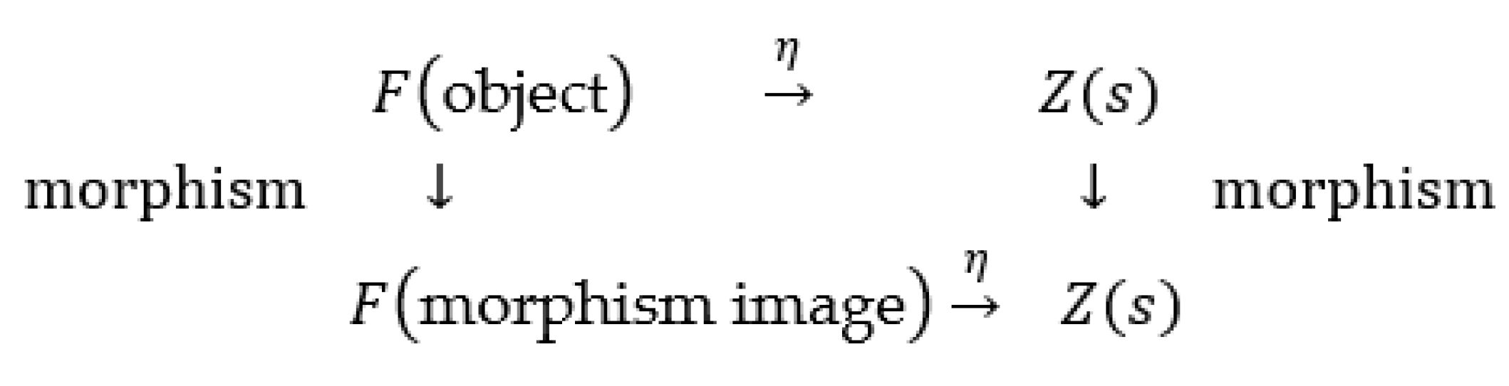
| Quantity | Expression (multi-component) |
|---|---|
| Grand-partition function | |
| Global gear mole fraction | |
| Critical composition per gear | |
| Integration constant per gear | |
| Interaction parameter per gear | |
| Lyapunov exponent per gear |
Table 2.
Thermodynamic potentials and heat capacities for Pressure–Volume Conjugate Pair [18].
Table 2.
Thermodynamic potentials and heat capacities for Pressure–Volume Conjugate Pair [18].
| Quantity | Expression |
|---|---|
| Gibbs free energy | |
| Molar Entropy | |
| Molar Enthalpy | |
| Molar Internal-energy | |
| Heat capacity at constant pressure | |
| Heat capacity at constant volume | |
| Pressure dome |
Table 4.
Formation Energies of Adsorbed Promoter Species on Ru and Co Surfaces [58].
Table 4.
Formation Energies of Adsorbed Promoter Species on Ru and Co Surfaces [58].
| Adsorbates | Li* | (LiO)* | (LiOH)* | Cs* | (CsO)* | (CsOH)* |
|---|---|---|---|---|---|---|
| Ru | -1.2 | -1.96 | -2.24 | -1.74 | -2.27 | -2.51 |
| Co | -0.91 | -1.73 | -2.1 | -1.51 | -2.01 | -2.37 |
| Adsorbates | Ba* | (BaO)* | (BaOH)* | Ca* | (CaO)* | (CaOH)* |
| Ru | -2.45 | -3.27 | -3.33 | -2.02 | -2.91 | -2.99 |
| Co | -1.96 | -2.93 | -3 | -1.45 | -2.67 | -2.73 |
| Adsorbates | La* | (LaO)* | (LaN)* | K* | (KO)* | (KOH)* |
| Ru | -2.72 | -3.77 | -2.65 | -1.51 | -2.1 | -2.24 |
| Co | -1.97 | -3.32 | -1.58 | -1.27 | -1.81 | -2.19 |
Table 5.
N Adsorption Energies and N–N Transition-State Energies on Pristine and Promoter-Doped Metal Surfaces Spin Polarized (SP) and Non-Spin Polarized (nSP) [58].
Table 5.
N Adsorption Energies and N–N Transition-State Energies on Pristine and Promoter-Doped Metal Surfaces Spin Polarized (SP) and Non-Spin Polarized (nSP) [58].
| Surfaces | E (eV) | Pristine (eV) |
Cs (eV) |
K (eV) |
Li (eV) |
Ba (eV) |
Ca (eV) |
La (eV) |
|---|---|---|---|---|---|---|---|---|
| Ru | -0.85 | -0.88 | -0.88 | - | -0.91 | -0.91 | -0.92 | |
| 0.169 | -0.007 | -0.006 | -0 | -0.122 | -0.101 | -0.119 | ||
| Rh | -0.4 | -0.443 | -0.443 | - | -0.459 | - | -0.445 | |
| 0.998 | 0.87 | 0.842 | - | 0.793 | - | 0.829 | ||
| Pd | 0.541 | 0.534 | 0.537 | - | 0.571 | - | 0.655 | |
| 2.343 | 2.247 | 2.225 | - | 2.231 | - | 2.273 | ||
| Co (SP) | -0.28 | -0.3 | -0.326 | - | -0.437 | -0.459 | -0.633 | |
| 1.042 | 0.716 | 0.687 | 0.524 | 0.408 | 0.339 | 0.122 | ||
| Co (nSP) | -1.05 | -1.082 | -1.075 | - | -1.08 | -1.068 | -1.068 | |
| 0.027 | -0.166 | -0.18 | -0.31 | -0.315 | -0.339 | -0.365 | ||
| Ni (SP) | -0.15 | -0.1 | - | - | -0.03 | - | -0.19 | |
| 1.677 | 1.244 | 1.218 | - | 1.033 | - | 0.826 | ||
| Ni (nSP) | -0.61 | -0.6 | -0.58 | - | -0.57 | - | -0.57 | |
| 0.856 | 0.638 | 0.618 | - | 0.496 | - | 0.427 |
Table 6.
Electric Field, Promotion Energy, and Transition-State Energy Lowering Induced by Promoters on Ru Surfaces [58].
Table 6.
Electric Field, Promotion Energy, and Transition-State Energy Lowering Induced by Promoters on Ru Surfaces [58].
| Promoter | Li | K | Cs | Ca | Ba | La |
|---|---|---|---|---|---|---|
| Electric field | -1.67 | -1.54 | -1.54 | -2.5 | -2.67 | -2.58 |
| (eV) | -0.16 | -0.15 | -0.15 | -0.24 | -0.26 | -0.25 |
| Calculated | -0.17 | -0.18 | -0.17 | -0.27 | -0.29 | -0.29 |
Table 7.
Electric Field, Promotion Energy, and Transition-State Energy Lowering Induced by Promoters on Co Surfaces [58].
Table 7.
Electric Field, Promotion Energy, and Transition-State Energy Lowering Induced by Promoters on Co Surfaces [58].
| Promoter | K | Cs | Li | Ba | Ca | La |
|---|---|---|---|---|---|---|
| Electric field | -1.67 | -1.53 | -1.88 | -2.05 | -2 | -2.25 |
| -0.26 | -0.24 | -0.29 | -0.32 | -0.31 | -0.35 | |
| Calculated | -0.35 | -0.33 | -0.52 | -0.63 | -0.7 | -0.92 |
Table 8.
Ammonia Synthesis Activity of Promoted Catalysts at Constant Pressure (10 bar) [58].
Table 8.
Ammonia Synthesis Activity of Promoted Catalysts at Constant Pressure (10 bar) [58].
| Catalyst | |||
|---|---|---|---|
| Ba-Ru-Li/AC | 10 | 459 | 46.3 |
| Li-Ru/(111)MgO | 10 | 400 | 33.04 |
| Cs-Ru/(111)MgO | 10 | 400 | 22 |
| Ba-Ru/AC | 10 | 400 | 8.285 |
| Cs-Ru/MgO | 10 | 400 | 12.117 |
| Cs–Ru/r-CeO2 | 10 | 400 | 14.266 |
| Ru/C12A7:e- | 10 | 400 | 8.245 |
| K–Ru/r-CeO2 | 10 | 400 | 11.227 |
| Co/CeO2-D-500 | 10 | 425 | 19 |
| Ru@CeO2-9 | 10 | 425 | 13.5 |
| Cs-Ru/BaCeO3-a (1.25wt%) | 10 | 425 | 14.57 |
| Ru−Ba/Al2O3-980 | 10 | 400 | 7.217 |
| Ru-Cs/MgO-MIL | 10 | 400 | 19.2 |
| Co–LiH | 10 | 350 | 11.2 |
| Ru/Pr2O3 | 10 | 400 | 19.1 |
| Ru/Ce0.6Zr0.42O2 | 10 | 390 | 1.7 |
| Ru/Ca2N:e- | 10 | 320 | 4 |
| 3BaH2-10%Co/CNTs | 10 | 400 | 21 |
| Ba-Co/C | 10 | 440 | 86.4 |
| KM1 | 10 | 440 | 46.8 |
| LaRuSi after EDTA | 10 | 400 | 14.3 |
| Co/C12A7:e− | 10 | 400 | 4.2 |
| Co-Mo/CeO2(NaNaph) | 10 | 400 | 3.15 |
| Ru/Ca(NH2)2 | 10 | 320 | 31.97 |
| Ru/Ba-Ca(NH2)2 | 10 | 340 | 57.05 |
| Co/Ba-Ca(NH2)2 | 10 | 380 | 24.42 |
| Ru/BaO−CaH2 | 10 | 320 | 30.66 |
| Ru/Ti-Ce-S | 10 | 400 | 14.58 |
| LaCoSi | 10 | 400 | 5.5 |
| Ru/3LaN/ZrH2 | 10 | 400 | 12.8 |
| Ni/CeN | 10 | 340 | 9 |
| Ni/LaN | 10 | 340 | 5.3 |
| Ru/Ba/LaCeOx | 10 | 400 | 88.1 |
Table 9.
Fe catalyst () — Traditional high-pressure operating window.
| 300 | 0.932 | 14.8 | 2145 | 0.412 |
| 350 | 0.857 | 10.2 | 1480 | 0.378 |
| 400 | 0.793 | 7.1 | 1030 | 0.341 |
| 450 | 0.739 | 5.0 | 725 | 0.302 |
| 500 | 0.691 | 3.6 | 522 | 0.261 |
Table 10.
Ru catalyst () — Shifted low-pressure operating window.
| P (MPa) | P (psia) | |||
|---|---|---|---|---|
| 300 | 0.932 | 5.9 | 856 | 0.465 |
| 350 | 0.857 | 4.1 | 595 | 0.431 |
| 400 | 0.793 | 2.8 | 406 | 0.392 |
| 450 | 0.739 | 2.0 | 290 | 0.349 |
| 500 | 0.691 | 1.4 | 203 | 0.303 |
Table 11.
Sensitivity of the Hessian scalar (proportional to the smallest positive eigenvalue ) to inert mole fraction at representative ammonia-synthesis conditions.
Table 11.
Sensitivity of the Hessian scalar (proportional to the smallest positive eigenvalue ) to inert mole fraction at representative ammonia-synthesis conditions.
| T (°C) | P (psia) | Inert Mole Fraction | Change in with Higher Inerts | |
|---|---|---|---|---|
| 327 | 400 | 1% | 0.420 | — |
| 327 | 400 | 11% | 0.337 | −20% |
| 327 | 800 | 1% | 0.438 | — |
| 327 | 800 | 11% | 0.348 | −21% |
| 427 | 400 | 1% | 0.507 | — |
| 427 | 400 | 11% | 0.393 | −22% |
| 427 | 800 | 1% | 0.582 | — |
| 427 | 800 | 11% | 0.441 | −24% |
Disclaimer/Publisher’s Note: The statements, opinions and data contained in all publications are solely those of the individual author(s) and contributor(s) and not of MDPI and/or the editor(s). MDPI and/or the editor(s) disclaim responsibility for any injury to people or property resulting from any ideas, methods, instructions or products referred to in the content. |
© 2026 by the author. Licensee MDPI, Basel, Switzerland. This article is an open access article distributed under the terms and conditions of the Creative Commons Attribution (CC BY) license (http://creativecommons.org/licenses/by/4.0/).
Copyright: This open access article is published under a Creative Commons CC BY 4.0 license, which permit the free download, distribution, and reuse, provided that the author and preprint are cited in any reuse.


