
Submitted:
10 July 2026
Posted:
13 July 2026
You are already at the latest version
Abstract
Recent advances in Micro-Electro-Mechanical Systems (MEMS) have enabled the development of accelerometers increasingly suitable for seismological and structural engineering applications. Quartz MEMS (QMEMS) sensors combine low self-noise, wide dynamic range, excellent thermal stability, and compact dimensions, providing a cost-effective alternative to conventional force-balance and piezoelectric accelerometers. This study presents the development and validation of a complete QMEMS-based sensing platform for seismic monitoring and Structural Health Monitoring (SHM), integrating the recently introduced Epson M-A370 accelerometer, a Smart Sensor Box with precise timing synchronization, embedded acquisition and edge-processing capabilities, and comprehensive laboratory and field validation. The M-A370 is evaluated against the previous-generation M-A352 and representative MEMS, piezoelectric, and force-balance accelerometers. Experimental results demonstrate that accelerometer self-noise is a primary factor governing the reliability of Operational Modal Analysis (OMA) and long-term SHM. Self-noise densities below 1 μg/√Hz, and preferably below 0.5 μg/√Hz, are shown to be necessary for robust modal identification and long-term tracking of structural dynamic properties under weak ambient excitation. The ultra-low-noise M-A370 (0.02 μg/√Hz) provides data quality comparable to engineering-grade force-balance accelerometers while enabling continuous monitoring of buildings, bridges, and heritage structures. The proposed sensing platform, combining ultra-low-noise QMEMS technology, precise timing synchronization, and embedded processing, provides a scalable framework for Urban Seismic Observatories, Operational Modal Analysis, distributed SHM systems and impact-based Earthquake Early Warning.
Keywords:
QMEMS accelerometers
; seismic monitoring
; structural health monitoring
; operational modal analysis
; urban seismic observatory
; smart sensor box
; impact-based earthquake early warning
1. Introduction
Accelerometric measurements play a fundamental role in both seismology and structural engineering, providing direct observations of ground and structural motion over a wide dynamic range, from weak ambient vibrations to strong earthquake shaking. In seismological applications, accelerometers are particularly important for near-field monitoring and engineering seismology, where large-amplitude motions must be recorded without clipping while preserving waveform fidelity and timing accuracy. These recordings are routinely used to derive engineering ground-motion parameters and intensity measures, including Peak Ground Acceleration (PGA), Peak Ground Velocity (PGV), Peak Ground Displacement (PGD), Arias Intensity, and response spectra [1,2]. These parameters constitute the basis for seismic hazard assessment, ShakeMap generation, rapid impact assessment, and modern Earthquake Early Warning (EEW) systems [3,4,5]. Beyond peak parameters such as PGA, PGV, and PGD, energy- and duration-based intensity measures derived from acceleration records are increasingly adopted to characterize earthquake shaking, evaluate structural response, and assess structural damage, particularly within performance-based earthquake engineering frameworks [2,6,7,8].
At the urban scale, the growing availability of compact digital instrumentation has promoted the development of Urban Seismic Networks (USNs) and Urban Seismic Observatories (USOs), designed to characterize spatial variations of ground motion with high resolution and to support rapid impact assessment and emerging impact-based EEW approaches. In Italy, representative examples include the Urban Seismic Observatory of Catania [9] and the more recent urban monitoring networks deployed in the Campi Flegrei, Messina–Reggio Calabria and Potenza.
Similar initiatives have been developed worldwide through the GeoNet strong-motion infrastructure in New Zealand [10,11], the K-NET and KiK-net networks in Japan [12], the metropolitan monitoring systems operated by the China Earthquake Administration [13,14], the SASMEX framework in Mexico [5,15], and the Community Seismic Network in the United States [16,17]. These experiences demonstrate a global transition toward dense, real-time, and impact-oriented seismic monitoring infrastructures.
Accelerometers are equally important in structural engineering, where they are deployed on buildings, bridges, towers, cultural heritage structures, and critical infrastructures to record ambient and earthquake-induced vibrations. Such measurements form the basis for Operational Modal Analysis (OMA) and Structural Health Monitoring (SHM), enabling the estimation and long-term tracking of modal parameters, including natural frequencies, damping ratios, and mode shapes. Temporal variations in these modal parameters may indicate changes in structural properties and therefore provide reliable vibration-based indicators for damage detection and structural integrity assessment [18,19,20,21].
Because many civil structures exhibit low-frequency vibration modes excited by extremely weak ambient motions, SHM applications impose stringent requirements on sensor performance, including ultra-low self-noise, excellent low-frequency resolution, long-term stability, and precise timing synchronization among distributed sensing nodes [20,21,22,23]. Traditionally, these applications have relied on high-performance force-balance accelerometers and conventional piezoelectric sensing technologies [23,24]. While both technologies provide excellent metrological performance, they generally involve higher costs, installation complexity, and maintenance requirements. Although these instruments remain reference solutions for many scientific and engineering applications, their widespread deployment in dense urban networks and distributed SHM systems is frequently constrained by economic and logistical considerations.
Recent advances in Micro-Electro-Mechanical Systems (MEMS) technology are progressively reshaping both seismological monitoring [9,25] and Structural Health Monitoring [18,20] by enabling compact, low-power, and cost-effective sensing systems suitable for large-scale deployments. Over the past decade, low-noise MEMS accelerometers have emerged as a promising alternative for Urban Seismic Networks, Operational Modal Analysis, distributed SHM systems, and edge-based Earthquake Early Warning architectures. Nevertheless, many conventional MEMS devices still exhibit limitations related to self-noise, thermal drift, low-frequency response, and long-term stability, particularly when employed for weak-motion monitoring and modal identification tasks.
Among the various MEMS technologies currently available, resonant Quartz MEMS (QMEMS) devices have recently attracted considerable attention because they combine the long-term stability and high mechanical quality factor of quartz resonators with highly integrated MEMS fabrication processes [26]. Within this technological framework, QMEMS accelerometers represent a significant evolution of MEMS accelerometry. Unlike conventional capacitive MEMS devices, they employ resonant quartz elements as acceleration-to-frequency transducers, thereby combining the scalability and compactness of MEMS fabrication with the excellent thermal stability, low hysteresis, and intrinsic frequency stability of quartz resonators. These characteristics provide ultra-low self-noise, high linearity, a wide dynamic range, and excellent long-term stability, making QMEMS accelerometers particularly attractive for weak- and strong-motion seismology, Operational Modal Analysis (OMA), and Structural Health Monitoring (SHM).
In this work, particular attention is devoted to the Epson M-A370 QMEMS accelerometer, released in 2025 as the latest evolution of the M-A352 sensor. The M-A370 incorporates several technological improvements aimed at enhancing performance in weak-motion seismology, ambient vibration monitoring, and Structural Health Monitoring applications. This study presents the laboratory characterization, shake-table experiments, and first field applications of the recently introduced M-A370 and complements these results with extensive long-term experience accumulated with the previous-generation M-A352. The performance of both sensors is compared with selected MEMS accelerometers, piezoelectric sensors, and reference-grade seismological instruments. Particular emphasis is placed on self-noise characteristics, timing performance, and their implications for Operational Modal Analysis and long-term SHM applications. The study additionally presents a multiparametric Smart Sensor Box specifically developed for seismic and SHM applications and discusses some representative implementations involving Urban Seismic Observatories, distributed SHM systems, bridge monitoring, cultural heritage structures, and impact-based Earthquake Early Warning. Collectively, these examples demonstrate how recent advances in low-noise QMEMS technology, combined with precise timing synchronization and embedded processing capabilities, enable a scalable sensing platform for next-generation distributed seismic and structural monitoring systems.
2. Accelerometric Sensors, Acquisition System, and Experimental Procedures
Recent advances in accelerometric technologies have progressively transformed both seismic monitoring and Structural Health Monitoring (SHM), enabling the transition from conventional force-balance and piezoelectric instruments to highly integrated MEMS-based solutions. Modern applications increasingly require sensors capable of simultaneously resolving weak ambient vibrations and strong earthquake motions while satisfying stringent requirements in terms of self-noise, dynamic range, bandwidth, timing synchronization, long-term stability, and deployment scalability. These requirements are particularly critical for Operational Modal Analysis (OMA), distributed SHM systems, Urban Seismic Observatories, and emerging impact-based Earthquake Early Warning applications. Within this context, Quartz MEMS (QMEMS) technology represents a significant evolution of microfabricated accelerometers, combining the scalability and low power consumption of MEMS devices with the excellent thermal stability and low-noise characteristics of quartz resonators. The following sections describe the accelerometers and reference instrumentation considered in this study, the multiparametric acquisition architecture specifically developed for seismic and SHM applications, and the laboratory and field experimental procedures adopted to evaluate sensor performance and representative application scenarios.
2.1. QMEMS Technology, and Reference Instrumentation
To provide a benchmark for evaluating the performance of the investigated QMEMS sensors, several representative MEMS, QMEMS, force-balance, and IEPE accelerometers commonly adopted in seismic and structural monitoring applications were considered. Most of the accelerometers listed in Table 1 and Table 2 were experimentally evaluated or deployed in the laboratory and field case studies presented in this work, covering both seismic monitoring and SHM applications. Figure 1 further compares the self-noise power spectral density (PSD) of a selection of these instruments, highlighting their relative noise performance over the frequency range of interest.
Force-balance accelerometers (FBAs) have long represented the reference technology for strong-motion seismology, engineering seismology, and high-performance vibration monitoring, including Operational Modal Analysis (OMA). By employing closed-loop servo mechanisms that maintain the proof mass near its equilibrium position, these instruments provide excellent linearity, stable low-frequency response, wide dynamic range, and very low self-noise [27]. Consequently, they are widely adopted in national and regional seismic networks, engineering seismology, and qualification procedures for strong-motion instrumentation [24,27,29]. Within the framework established by the Advanced National Seismic System (ANSS), Class-A systems are characterized by very high useful resolution and dynamic range, typically exceeding 110 dB [29].
Piezoelectric accelerometers, including IEPE devices, have long represented a reference technology for vibration testing, OMA analysis, and industrial monitoring owing to their robustness, high sensitivity, low noise, and excellent high-frequency response [30,31]. However, because of their intrinsically AC-coupled nature, they do not provide a true DC response and are therefore less suitable for very-low-frequency and quasi-static measurements [32]. In addition, wiring requirements, power consumption, and installation complexity may limit their applicability in dense and distributed monitoring networks. For these reasons, increasing attention has recently been devoted to low-noise MEMS and QMEMS technologies, which combine DC response, low power consumption, compact size, and ease of integration with embedded processing and wireless communication systems.
The rapid development of Micro-Electro-Mechanical Systems (MEMS) technology has introduced compact and cost-effective accelerometers suitable for different applications and large-scale deployments. Capacitive MEMS sensors estimate acceleration through displacement-induced variations in differential capacitance [25], whereas piezoresistive MEMS devices exploit strain-induced resistance variations and are commonly employed in high-g and shock applications [33]. Their capability to provide response down to DC makes MEMS accelerometers particularly attractive for dense Urban Seismic Networks and SHM systems [17,22,34].
Figure 1 shows that, despite their advantages in terms of cost and scalability, conventional MEMS accelerometers may exhibit self-noise levels significantly higher than those of force-balance accelerometers and velocimetric seismometers. These limitations become particularly important for weak-motion seismology, Operational Modal Analysis (OMA), and long-term Structural Health Monitoring applications, where the ability to resolve signals close to the ambient noise level is essential.
The fundamental differences between conventional capacitive MEMS and quartz-resonant MEMS accelerometers are schematically illustrated in Figure 2. Conventional capacitive MEMS sensors measure acceleration through displacement-induced variations in differential capacitance, which are subsequently converted into electrical signals. As illustrated in the upper part of Figure 2, this measurement chain relies on analog signal conditioning and analog-to-digital conversion stages that inherently introduce trade-offs among resolution, dynamic range, and linearity. Furthermore, achieving stable low-frequency performance, particularly from DC to a few hertz, remains difficult because of 1/f noise, thermal drift, and long-term instabilities affecting both the sensing element and the analog front-end.
Quartz-resonant MEMS (QMEMS) accelerometers adopt a fundamentally different sensing principle, illustrated in the lower part of Figure 2. Instead of directly measuring proof-mass displacement, these devices employ a Double-Ended Tuning Fork (DETF) quartz resonator as the sensing element. Acceleration applied to the proof mass generates axial stress within the resonator, producing a measurable shift in its resonant frequency. This acceleration-to-frequency conversion approach provides a highly linear output that can be processed digitally with very high precision, reducing the influence of analog conditioning electronics and minimizing quantization and linearity limitations commonly associated with conventional readout chains [36].
In this configuration, the achievable dynamic range is primarily governed by the frequency measurement system rather than by the analog conversion stage. In the following, we describe the characteristics of the Epson M-A370 QMEMS accelerometer (Figure 3a), a new-generation device developed as an evolution of the widely adopted M-A352 platform [37].
The M-A370 was specifically designed to improve sensitivity to weak ground motions and ambient structural vibrations, which are key requirements for modern seismic monitoring, Operational Modal Analysis (OMA), and Structural Health Monitoring applications.
One of the principal factors contributing to the improved performance of the M-A370 is the increase in transducer sensitivity obtained through the adoption of a high-density tungsten proof mass, replacing the phosphor-bronze mass employed in the previous generation. As shown in Figure 3b, this design modification substantially increases inertial mass while preserving the compact dimensions of the sensor. Combined with an optimized DETF geometry derived through finite-element modeling, this configuration increases acceleration sensitivity from approximately 152 Hz/g in the M-A352 to approximately 550 Hz/g in the M-A370. Such an improvement enhances the capability of resolving extremely weak acceleration signals associated with microtremors, ambient vibrations, and weak-motion seismic recordings.
To exploit this increased sensitivity while maintaining robustness under field conditions, the M-A370 adopts a differential architecture consisting of six DETF resonators arranged as three independent pairs, one for each measurement axis (Figure 3b). In contrast to previous single-ended implementations, the differential configuration measures the frequency difference between paired resonators operating in a push-pull mode. This approach suppresses common-mode effects associated with temperature variations, packaging-induced stresses, and other environmental perturbations, resulting in improved bias stability and scale-factor consistency over a broad operating temperature range.
Further improvements are achieved through a fully digital frequency-measurement architecture based on a proprietary phase-measurement approach inspired by moiré-pattern sensitivity [38]. Implemented on a low-power FPGA platform, the system measures resonant-frequency variations with high precision while avoiding several sources of nonlinearity typically associated with conventional analog phase detectors and reciprocal frequency counters.
As a result of these combined mechanical and electronic developments, the M-A370 achieves a noise density of approximately 0.02 µg/√Hz in the 1–10 Hz frequency band. Such performance approaches the levels traditionally associated with high-end force-balance accelerometers and enables applications that have historically required more expensive instrumentation and, in some cases, also velocimeters. Representative examples include microtremor array measurements, H/V spectral-ratio analysis, weak-motion seismology, and long-term Structural Health Monitoring.
These characteristics are relevant for dense Urban Seismic Networks and in particular for SHM systems [9,39] where the capability to resolve signals close to the ambient noise level directly influences the quality of modal identification, ambient-vibration analysis, and weak-earthquake recordings. More generally, the evolution from conventional MEMS architectures toward quartz-resonant technologies reflects the broader trend toward sensing platforms capable of combining the metrological performance traditionally associated with force-balance accelerometers with the scalability, compactness, and deployment flexibility required by next-generation seismic and structural monitoring systems.
2.2. Multiparametric Smart Sensor Box and Timing Architecture
To evaluate the performance of the Epson M-A352 and M-A370 QMEMS accelerometers for seismic monitoring and Structural Health Monitoring (SHM) applications, a multiparametric Smart Sensor Box was developed by further extending a previously proposed architecture [40]. The updated platform, implemented in 2025 in collaboration with specialized industrial partners, was employed throughout the laboratory investigations presented in this work.
The Smart Sensor Box relies on a fully digital and modular acquisition architecture specifically conceived for seismic and SHM applications and supporting multi-parameter environmental monitoring. As illustrated in Figure 4, the system integrates high-sensitivity QMEMS accelerometers, a GNSS-disciplined Time Base Unit (TBU), a dual-core STM32H7 microcontroller (MCU), an embedded Single Board Computer (SBC), communication interfaces, local storage capabilities, and auxiliary sensors. The architecture enables the integration of accelerometers, GNSS receivers, inclinometers, environmental sensors, and other digital sensing devices commonly adopted in distributed monitoring networks. Although the present study focuses on Epson QMEMS accelerometers, the acquisition, synchronization, and processing framework is sensor-independent and can be readily adapted to alternative sensing technologies.
Sensor acquisition, buffering, and communications are managed by the dual-core STM32H7 microcontroller, whereas timing synchronization is provided by the dedicated Time Base Unit. Building upon the previously proposed architecture [40], the system separates high-rate dynamic measurements from environmental and diagnostic data streams, allowing vibration measurements and auxiliary parameters to be acquired independently while preserving deterministic timing and low timing jitter. This approach enables vibration measurements to be acquired with precise temporal control while simultaneously collecting environmental and diagnostic parameters such as temperature, humidity, atmospheric pressure, inclination, power-system information, and GNSS data.
The timing subsystem is based on a GNSS-disciplined oscillator and a dedicated Time Base Unit (TBU), which provide a common and highly stable time reference, enabling all sensing nodes to remain accurately synchronized. Rather than distributing synchronization signals to remote sensors, the architecture ensures that all nodes operate with the same timing reference and maintain a high degree of temporal consistency. Such synchronization is essential for seismic monitoring, Operational Modal Analysis (OMA), vibration-based damage detection, wavefield analysis, and other distributed measurement applications requiring sub-millisecond timing accuracy.
Moreover, the Smart Sensor Box combines the capabilities of the dual-core microcontroller with those of the embedded Single Board Computer (SBC), providing on-board signal processing, data-quality control, event detection, local data storage, and edge-computing capabilities. The SBC supplies the computational resources required for advanced functionalities, including impact-based Earthquake Early Warning (EEW), strong-motion parameter estimation, local classification algorithms, and real-time generation of graphical products. As a whole, the proposed architecture constitutes a flexible and scalable platform for distributed seismic monitoring and Structural Health Monitoring systems, paving the way for future developments toward Urban Seismic Observatories, digital-twin applications, and the monitoring of critical infrastructures and cultural heritage assets. Figure 4 illustrates the functional architecture of the multiparametric Smart Sensor Box employed throughout this study.
2.3. Experimental Setups
Laboratory and field experiments were carried out to characterize the performance of the investigated sensors under conditions representative of both seismological and Structural Health Monitoring (SHM) applications. The experimental campaign comprised laboratory calibration and dynamic shake-table tests, timing validation under both GNSS-disciplined and GNSS-denied conditions, and long-term field deployments involving urban seismic observatories, bridge monitoring, building monitoring, and cultural heritage structures.
Laboratory experiments were performed at the L.E.D.A. (Laboratory of Earthquake Engineering and Dynamic Analysis) Research Centre of the University of Enna “Kore” using a SPEKTRA CS18P vibration calibration system equipped with an APS 129 electrodynamic shaker featuring hydrodynamic suspension and closed-loop motion control. The calibration system supports secondary calibration procedures compliant with ISO 16063-21 and provides programmable, low-distortion sinusoidal excitation over a broad frequency and velocity range. Under these controlled laboratory conditions, the Epson M-A352 and M-A370 QMEMS accelerometers, together with a reference Güralp Fortimus force-balance accelerometer, were tested using identical excitation sequences to enable a direct comparison of their dynamic performance.
The laboratory characterization consisted of sinusoidal excitation tests covering frequencies between 0.5 and 100 Hz and nominal peak acceleration amplitudes ranging from 0.1 to 5 m s⁻², according to the operating range of the investigated sensors and the capabilities of the calibration system. The recorded waveforms were analysed using an automated processing workflow specifically developed for this study. The adopted signal-processing procedure is described in Section 3.1.
To complement the calibration tests, the results of a comparative dynamic testing campaign performed on the 2:3 scale masonry building installed on one of the two large-scale shaking tables of the L.E.D.A. Research Centre are also presented [41]. The experimental facility enables controlled seismic excitation of large structural specimens under realistic dynamic loading conditions. During this experiment, a total of 34 sensors (92 channels), including Epson M-A352 QMEMS, Safran-Colibrys VS1002, Analog Devices ADXL355, and PCB Piezotronics 356A17 accelerometers, were deployed to investigate their performance and the capability of different sensing technologies to identify also the modal properties of the structure.
Timing performance was evaluated through laboratory and field experiments involving pairs of co-located Smart Sensor Boxes operating under both GNSS-disciplined and GNSS-denied conditions. Oscilloscope measurements, phase analysis, coherence estimates, and sub-sample cross-correlation techniques were employed to quantify synchronization accuracy and relative timing stability. The adopted experimental procedures and the corresponding results are presented in Section 3.3.
Finally, several long-term field deployments were carried out to assess the suitability of the proposed low-noise QMEMS accelerometers for real-world applications. These included Urban Seismic Observatories in southern Italy, monitoring systems deployed on residential buildings in the Campi Flegrei area, continuous monitoring of the Ragusa Bridge, and permanent and temporary deployments at the Bell Tower of the Basilica of Saint Francis in Assisi and at Durham Castle, both UNESCO World Heritage sites, to support Operational Modal Analysis (OMA) investigations.
3. Results
3.1. Laboratory Evaluation of Sensor Performance
The laboratory validation presented in this section aims to assess the amplitude accuracy, linearity, and repeatability of the proposed acquisition systems over the frequency range relevant to seismic monitoring and Structural Health Monitoring (SHM) applications. Figure 5 illustrates the three experimental configurations adopted during the laboratory validation. First, the complete Smart Sensor Boxes integrating the Epson M-A352 and M-A370 QMEMS accelerometers were tested in their operational configuration (Figure 5a). In the second configuration (Figure 5b), the sensing elements alone were mounted directly on the shaker table and connected through shielded cables to the corresponding Smart Sensor Boxes positioned outside the shaker. This arrangement was adopted exclusively for the laboratory experiments to isolate the intrinsic response of the sensing elements from the eventual mechanical influence of the enclosure. Both accelerometers were evaluated using the same acquisition electronics and identical signal-processing chain, with all signals synchronously acquired at 500 samples per second (sps) using the sensors’ built-in 210 Hz low-pass filter. Finally, the Güralp Fortimus, integrating the force-balance accelerometer, digitizer, and acquisition electronics into a single instrument, was mounted directly on the shaker table (Figure 5c), tested under the same excitation conditions, and used as the reference instrument.
The experimental program consisted of sinusoidal excitations at frequencies of 0.5, 1, 2, 10, 20, 50, and 100 Hz, combined with nominal peak acceleration amplitudes of 0.1, 0.5, 1, 3, and 5 m s⁻² (Figure 5d). For each excitation condition, the calibration system generated the prescribed reference motion while the output signals from the three acquisition systems were recorded for subsequent analysis.
To ensure a consistent, objective and fully reproducible evaluation of sensor performance all recorded waveforms were processed using an automated Python workflow specifically developed for this study. Because each excitation record included transient phases associated with the stabilization of the vibration calibration system following changes in excitation frequency or amplitude, the first step consisted of identifying the stationary portion of the signal before quantitative analysis. Each waveform was divided into consecutive 10 s windows, which were mean-corrected, detrended, and tapered using a Gaussian window prior to frequency-domain analysis. Stable windows were automatically identified according to predefined frequency- and amplitude-consistency criteria, and the longest continuous stationary interval was retained for further processing.
The selected waveform was subsequently analysed using a fixed-frequency least-squares sine fit to estimate the measured acceleration amplitude, excitation frequency, phase, and residual offset. The fully automated workflow ensured identical processing of all datasets without user intervention, thereby enabling a reproducible and unbiased comparison of the investigated acquisition systems.
Figure 6a-c summarize the laboratory validation results obtained for the three configurations. Figure 6a and Figure 6b present the results for the QMEMS M-A370 sensor. The corresponding results for the M-A352 were nearly identical and are therefore omitted for brevity. All configurations accurately reproduce the applied sinusoidal motion over the investigated frequency range. The measured amplitudes remain in close agreement with the nominal excitation values, with deviations generally within the uncertainty limits of the calibration system. Moreover, no significant dependence of the amplitude error on the excitation level is observed, indicating that all acquisition systems preserve a linear response throughout the investigated dynamic range.
A modest increase in the measured amplitude error is observed at the highest test frequencies, particularly approaching 100 Hz. Because a comparable trend is evident for all tested configurations, including the reference force-balance accelerometer, this behaviour is unlikely to originate from the intrinsic response of the sensing elements. Instead, it is more plausibly associated with the experimental conditions, including the dynamic characteristics of the vibration calibration system, the mounting fixtures and sensor supports, as well as other sources of high-frequency mechanical disturbance within the laboratory environment. Nevertheless, the observed deviations remain limited to a few percent and are therefore considered negligible for the intended applications.
Overall, excluding the expected limitations observed at the margins of the investigated frequency range, both QMEMS-based acquisition systems demonstrate excellent linearity, accuracy, and repeatability over the operational bandwidth relevant to seismic monitoring and Structural Health Monitoring applications.
Since the frequency content of interest for these applications is predominantly concentrated below 50 Hz, the experiments demonstrate that the proposed acquisition systems faithfully reproduce the reference motion throughout the operational bandwidth addressed in this work. Furthermore, no significant differences were observed between the first-generation architecture based on the externally connected M-A352 sensor and the second-generation integrated M-A370 configuration, demonstrating that integrating the sensing element within the acquisition unit does not compromise metrological performance while providing a more compact and robust architecture for long-term monitoring applications. These results demonstrate that the proposed QMEMS-based acquisition systems—and particularly the second-generation M-A370 configuration—achieve a metrological performance comparable to that of the reference force-balance instrument over the frequency band relevant to seismic and Structural Health Monitoring (SHM) applications, supporting their use in both permanent seismic monitoring networks and research-grade structural monitoring systems.
To complement the laboratory calibration tests, the performance of the investigated sensing technologies was further evaluated through a comparative dynamic testing campaign conducted in 2024 on a 2:3 scale masonry building installed on one of the two large-scale shaking tables at the L.E.D.A. Research Centre [41]. The structure was subjected to progressively increasing shaking levels reproduced from the ground motion recorded during the 6 April 2009 Mw 6.3 L’Aquila earthquake. A total of 34 sensors (92 channels), including Epson M-A352 QMEMS, Safran Colibrys VS1002, Analog Devices ADXL355, and PCB Piezotronics 356A17 accelerometers, were deployed on the structure, providing a unique benchmark for comparing different sensing technologies under both ambient-vibration and strong-motion conditions.
Although all sensors adequately reproduced the structural response during the shake-table excitations, significant differences emerged under low-amplitude conditions relevant to Operational Modal Analysis. Owing to their lower self-noise, the M-A352 QMEMS and the PCB Piezotronics 356A17 sensors provided the clearest stabilization diagrams and the most robust identification of the principal modal frequencies. In contrast, the VS1002 and, particularly, the ADXL355 exhibited a reduced capability to resolve weak structural modes, highlighting the critical role of self-noise in SHM and OMA applications.
As illustrated in Figure 7, these observations are fully consistent with the self-noise characteristics discussed in Section 2 and demonstrate that, for Operational Modal Analysis and long-term Structural Health Monitoring applications, self-noise densities below approximately 1 μg/√Hz—and preferably below 0.5 μg/√Hz—are essential for reliable modal identification and long-term tracking of structural dynamic properties.
3.2. Timing Synchronization Performance
Accurate timing synchronization is a key requirement for seismic monitoring, Operational Modal Analysis (OMA), and distributed Structural Health Monitoring (SHM) systems. In particular, applications involving phase measurements, transfer-function estimation, modal identification, and array processing demand a high degree of phase coherence and, in many cases, sub-millisecond synchronization accuracy [43,44,45,46]. Table 3 summarizes the typical synchronization requirements associated with representative applications in seismic monitoring, OMA, and SHM. The reported values represent practical engineering guidelines derived from published studies on modal identification, distributed sensing networks, and seismic monitoring systems [20,43,44,45,46].
However, the required timing accuracy depends on the frequency range of interest and on the sensitivity of the target parameters to phase and synchronization errors [42].
To assess the timing capabilities of the proposed Smart Sensor Box, a series of laboratory and field experiments was carried out under both GNSS-disciplined and GNSS-denied conditions. The experimental investigations included direct oscilloscope measurements of the 1PPS signals, characterization of the holdover behavior, and waveform-based analyses based on phase estimation, coherence analysis, and sub-sample cross-correlation techniques.
3.2.1. GNSS-Disciplined Operation
Under standard operating conditions, synchronization among sensing nodes is maintained through the GNSS-disciplined Time Base Unit described in Section 2.2. To evaluate the temporal performance of the proposed architecture, a series of laboratory and field experiments was conducted under both GNSS-disciplined and GNSS-denied operating conditions.
Laboratory tests were first performed to characterize the timing subsystem independently of the sensing chain. Direct oscilloscope measurements of the PPS signals revealed a relative timing difference of only approximately 54 ns between two independent GNSS receivers, while the timing offset between the GNSS-derived PPS and the synthetic PPS generated by the acquisition unit was approximately 14.2 μs. Holdover experiments (Figure 8) further demonstrated that, once GNSS synchronization is removed, timing stability is primarily controlled by the frequency stability of the local oscillator and its temperature dependence. These measurements confirm that the timing architecture is capable of maintaining microsecond-level synchronization during GNSS-disciplined operation while providing a stable timing reference during short-term GNSS outages. During the approximately 4.4 h holdover experiment, the relative timing error remained within ±80 μs, demonstrating good short-term stability under GNSS-denied conditions. For comparison, the timing difference between the PPS signals generated by two independent GNSS receivers was approximately 62.5 ns.
Synchronization performance was further assessed through coherence and cross-correlation analyses of simultaneously recorded vibration signals acquired from the N–S components of two co-located Smart Sensor Boxes.
A dedicated processing workflow combining Welch coherence estimation, phase analysis and sub-sample cross-correlation interpolation was developed to estimate relative timing offsets with a resolution significantly finer than the sampling interval. Synchronization tests performed on simultaneously operating GNSS-disciplined nodes revealed residual relative timing offsets of only a few microseconds, typically below 10 μs (Figure 9). At a sampling frequency of 1000 Hz, this corresponds to approximately 0.01 sample, confirming sub-sample temporal alignment between acquisition units.
The results indicate very high coherence and excellent agreement between the two independent estimation techniques. Similar behavior was observed for different components and frequency bands. Experiments were performed at both 200 and 1000 Hz sampling frequencies. At 200 Hz, relative delays estimated through sub-sample techniques generally remained within a few tens of microseconds and exhibited excellent temporal stability. Comparable results were obtained at 1000 Hz, although the higher sampling frequency made the phase and cross-correlation estimates more sensitive to the selected bandwidth and signal characteristics. As illustrated in Figure 9, coherence values close to unity and very small phase-derived lags demonstrate the capability of the proposed timing architecture to provide synchronization accuracies fully compatible with distributed seismic monitoring, array processing, and Operational Modal Analysis applications.
The results obtained under GNSS-disciplined conditions indicate excellent phase coherence and sub-millisecond synchronization, with relative timing offsets typically below 10 μs. Such performance satisfies the requirements of a wide range of seismic monitoring, Structural Health Monitoring, and vibration-based applications, and demonstrates the effectiveness of the adopted Time Base Unit architecture.
The achieved timing accuracy is comparable to that required for distributed vibration measurements and array-based analyses, confirming the suitability of the proposed system for applications requiring high temporal consistency among sensing nodes.
3.2.2. GNSS-Denied Conditions
For dynamic identification measurements associated with Structural Health Monitoring applications, sensors are frequently deployed inside buildings, underground environments, and cultural heritage structures where continuous GNSS reception cannot always be guaranteed. In these scenarios, preserving synchronization stability after the temporary loss of the external reference becomes a key requirement, particularly for Operational Modal Analysis (OMA), phase measurements, and transfer-function estimation.
To investigate this aspect, a series of experiments was carried out using pairs of co-located Smart Sensor Boxes operating under GNSS-denied conditions, complementing the tests previously performed under GNSS-disciplined operation. Two identical acquisition units (CT02 and CT04) were initially synchronized through GNSS and subsequently operated in holdover mode for more than 32 h. Relative timing offsets were estimated through phase analysis and sub-sample cross-correlation techniques applied to transient signals and ambient vibrations. The results summarized in Figure 10 and Table 4 confirm that the observed drift is governed by the combined effects of oscillator holdover characteristics and temperature-dependent frequency variations.
Following GNSS disconnection, the timing error remained limited to a few hundred microseconds during the first hours of operation, corresponding to only a small fraction of the sampling interval even at acquisition rates between 200 and 1000 Hz. The temporal evolution of the delay exhibits a smooth and progressive behavior rather than abrupt variations, indicating that the observed drift is primarily controlled by the intrinsic stability of the local oscillator and its temperature dependence. Such timing offsets have a negligible impact on modal parameter estimation and phase-based analyses.
Figure 10 provides additional insight into the holdover behavior by comparing the drift rate of the CT02–CT04 timing offset with the external ambient temperature measured by the Bosch BME280 sensor. Although the cumulative timing drift increased from less than 0.5 ms on 11 June to nearly 10 ms on 12 June, the corresponding drift rate remained within the same order of magnitude, generally below ±500 μs h⁻¹. This observation suggests that the frequency stability of the local oscillator remained relatively constant during prolonged holdover operation, while the absolute timing error progressively accumulated over time. The comparison with ambient temperature further indicates that thermal variations contribute to the observed drift evolution, although the relationship appears nonlinear and partially hysteretic.
Consequently, after an initial GNSS synchronization phase, the proposed system can be effectively deployed also for temporary monitoring campaigns (1-2 h) inside buildings and infrastructures where continuous GNSS reception is unavailable. For typical OMA surveys lasting one to two hours, the accumulated drift remains well below the synchronization requirements commonly adopted for modal identification and SHM applications, providing sufficient temporal stability for distributed measurements without permanent GNSS visibility at each sensing node.
Over longer periods, however, the cumulative timing error progressively increases, reaching approximately 10 ms after about 24 h of autonomous operation (Figure 10 and Table 4), consistent with the expected behavior of a standard VCXO operating in holdover mode. While the measured performance is fully compatible with temporary indoor monitoring campaigns lasting several hours after an initial GNSS synchronization phase, it becomes less suitable for long-duration distributed OMA and SHM measurements under prolonged GNSS-denied conditions.
The current Sensor Box architecture, based on a standard VCXO oscillator characterized by a frequency stability of several tens of ppm, already provides adequate timing stability for many seismic monitoring, OMA, and short-term SHM applications. Future developments will investigate the adoption of high-stability temperature-compensated oscillators (TCXO) exhibiting frequency stabilities as low as ±0.05 ppm (50 ppb). Such devices would improve frequency stability by approximately three orders of magnitude, significantly reducing temperature-induced frequency variations and extending holdover performance during prolonged GNSS outages. Under these conditions, the timing drift accumulated over several hours is expected to be reduced to the order of a few tens of microseconds, further enhancing the suitability of the proposed architecture for long-duration distributed OMA and SHM measurements.
4. Field Applications and Emerging Monitoring Frameworks
4.1. Urban Seismic Observatories and Impact-Based Earthquake Early Warning
The deployment of dense Urban Seismic Observatories (USOs) represents one of the most promising applications of modern low-noise QMEMS accelerometers. Since 2022, several urban seismic monitoring networks have been developed in southern Italy with the aim of improving the characterization of local seismic response, investigating the spatial variability of ground shaking, and supporting innovative approaches to Structural Health Monitoring and impact-based Earthquake Early Warning. Figure 11 summarizes the spatial distribution of the investigated urban seismic observatories and monitoring networks.
Among the urban infrastructures realized in southern Italy, the most recent Messina–Reggio Calabria Urban Seismic Network represents the largest homogeneous deployment based on Epson M-A352 QMEMS accelerometers, comprising 38 stations predominantly installed in strategic buildings and schools.
This dense configuration provides a unique framework for investigating local ground-motion variability and for the development of impact-based Earthquake Early Warning and distributed Structural Health Monitoring applications.
As previously reported for the Catania Urban Seismic Observatory [9], comprising 22 seismo-accelerometric stations, the lower self-noise of the Epson M-A352 resulted in significantly higher signal-to-noise ratios than those obtained with co-located Analog Devices ADXL355 MEMS accelerometers. Consequently, the M-A352 generally provides clearer phase arrivals and more reliable extraction of early-warning parameters over a broad range of earthquake magnitudes and source distances. However, the observed signal quality ultimately depends on earthquake magnitude and depth, propagation effects, and local site conditions. Owing to the frequent microseismic activity of Mt. Etna, local earthquakes with magnitudes of approximately ML 2.0 are readily detected by the network, with clear P- and S-wave arrivals observed at epicentral distances of 5–10 km. Events of approximately ML 3.0 can also be reliably detected and characterized at distances of several tens of kilometres, enabling robust estimation of early-warning parameters from the first seconds of the recordings.
Following, the same QMEMS sensors have been employed in the other urban seismic observatories and in several Structural Health Monitoring applications involving buildings, bridges, dams, and cultural heritage structures, further demonstrating their capability to accurately record both weak and strong motions.
An example is provided by the Campi Flegrei Urban Seismic Observatory [41], established in 2024 in response to the ongoing bradyseismic unrest affecting the caldera. Owing to its predominantly shallow seismicity, with most earthquakes occurring at depths of less than 3 km, and the frequent occurrence of low-magnitude events, the Campi Flegrei area represents an ideal natural laboratory for assessing weak-motion monitoring capabilities. Continuous recordings acquired by the M-A352 QMEMS stations exhibit excellent signal-to-noise ratios, enabling the reliable detection and recording of local earthquakes with magnitudes around Md 1.0 and below (Figure 12).
The recorded waveforms exhibit a quality comparable to that of co-located broadband seismometers and force-balance accelerometers operated by INGV–Osservatorio Vesuviano and the Italian National Accelerometric Network (RAN), further validating the use of low-noise QMEMS technology for high-resolution seismic monitoring in complex urban volcanic environments with elevated ambient noise levels. Together with the permanent INGV-OV and RAN stations, the OCF network currently forms one of the densest urban strong-motion monitoring systems operating in Italy.
This dense configuration provides a unique framework for investigating local ground-motion variability and for the development of impact-based Earthquake Early Warning and distributed SHM applications.
These dense urban monitoring systems provide information that complements conventional seismic microzonation studies. However, while seismic microzonation provides essential static information for territorial planning, Urban Seismic Observatories directly measure the actual spatial distribution of earthquake shaking within the built environment and provide the real-time information required for rapid impact assessment. Consequently, Urban Seismic Observatories represent a natural convergence point between seismology and structural engineering. As example, this capability is illustrated by the analysis of recordings acquired by the Messina–Reggio Calabria Urban Seismic Network during the recent deep Mw 6.1 Tyrrhenian earthquake of June 2026. Despite similar hypocentral distances of approximately 270–280 km, the stations exhibited significant variability in recorded amplitudes, highlighting the influence of local geological conditions and site effects. In particular, peak ground acceleration was dominated by the vertical component, consistent with the large focal depth of the event, whereas peak ground velocity showed a more balanced contribution from the three components and proved to be more representative of the ground shaking experienced across the urban area. Figure 13 summarizes the spatial distribution of the observed PGA and PGV values and illustrates the capability of the network to resolve local differences in ground motion at urban scale over relatively short distances. These observations demonstrate how real-time dynamic recordings can directly capture local amplification effects and spatial variability of ground shaking that may not be fully resolved by conventional microzonation studies. Consequently, Urban Seismic Observatories provide a valuable framework for understanding the interaction between earthquakes and the built environment and for improving the seismic resilience of urban areas.
The aforementioned urban seismic observatories are currently being used to test the proposed impact-based Earthquake Early Warning algorithm (PSAVE), which builds upon the methodologies previously proposed in [47,48] while incorporating several methodological improvements. Unlike conventional source-based EEW approaches, the adopted strategy combines rapid source characterization with the direct estimation of expected shaking and impact parameters, providing information more closely related to the potential effects on structures and infrastructures.
Figure 14 illustrates representative graphical products generated by the PSAVE system for station ME016 of Messina Urban Seismic Observatory network during the deep Mw 6.1 earthquake. For each station of the network the system automatically provided real-time estimates of intensity, alert level, engineering-impact indicators, observed PGA and PGV values, pseudo-spectral acceleration curves, other engineering parameters, and three-component acceleration time histories. The figure highlights both the capability of the system to capture local variations in ground shaking and its progressive transition from predictive EEW estimates to direct impact characterization.
The local implementation of PSAVE has been facilitated by the Smart Sensor Box architecture described in Section 2.2, which combines very low-noise QMEMS accelerometers, precise timing synchronization, and embedded processing capabilities. Through the combined use of the dual-core microcontroller and the embedded Single Board Computer, event detection, strong-motion parameter estimation, and preliminary impact assessment can be also performed locally, enabling edge-computing approaches and reducing communication requirements.
To reduce latency, reliable progressive alerts can be transmitted a few seconds (2, 3, 5 , 10 s) after the initial detection of P waves without graphical products, whereas complete strong-motion and EEW summaries can be subsequently generated using the transmitted waveform portions. Strong-motion parameters are progressively updated during the evolution of the event, providing increasingly reliable estimates of PGA, PGV, and macroseismic intensity. This approach represents a shift from conventional centralized architectures toward distributed intelligent sensing systems capable of performing local processing and decision support directly at the edge.
In summary, the combination of dense Urban Seismic Observatories, low-noise QMEMS accelerometers, accurate timing synchronization, and embedded processing capabilities provides a scalable framework for strong-motion monitoring, impact-based Earthquake Early Warning, and future digital-twin applications for urban areas and critical infrastructures.
4.2. Structural Health Monitoring Applications
Building upon the experience gained from Urban Seismic Observatories, the same low-noise QMEMS technology and Smart Sensor Box architecture have progressively been extended to Structural Health Monitoring (SHM) applications involving ordinary buildings, critical infrastructures, and cultural heritage structures. Experimental and field observations consistently demonstrate that accelerometer self-noise is one of the primary factors governing sensor selection and suitability for modal properties identification. Under ambient excitation conditions, structural responses are often only a few micro-g above the background noise level, and the reliable identification and long-term tracking of modal properties strongly depend on the instrumental noise floor. This crucial aspect emphasizes that force-balance accelerometers, piezoelectric sensors, QMEMS devices, and selected classes of low-noise MEMS sensors are suitable when adequate noise performance is achieved. As discussed in Section 3.1, these effects were clearly observed during the dynamic testing campaign carried out on the 2:3 scale masonry building at the L.E.D.A. laboratory [41]. Subsequent comparisons between the M-A352 and an early prototype of the M-A370 highlighted the advantages associated with the lower self-noise of the new-generation sensor. These improvements were particularly evident for weak-vibration measurements performed on structures characterized by extremely low-amplitude responses and located in very quiet environments, where the recorded signals approached the instrumental noise floor of the M-A352 [40].
Additional evidence was provided by the recent experimental campaign carried out at Durham Castle (United Kingdom), a UNESCO World Heritage masonry structure characterized by geometric complexity, very low vibration amplitudes, and the coexistence of global and local structural modes. During the campaign, a temporary network comprising ten stations equipped with next-generation M-A370 QMEMS accelerometers was deployed throughout the castle using multiple measurement layouts. This strategy enabled Operational Modal Analysis under ambient excitation conditions and the identification of both global and local vibration modes of the structure. Side-by-side measurements performed at the base and at the top of the clock tower (Figure 15) demonstrated the benefits associated with the lower self-noise of the new-generation device (Figure 1).
As shown in Figure 16, power spectral densities computed from one hour of ambient-noise recordings clearly reveal amplified structural resonances between approximately 2 and ~10 Hz at the top of the tower. Under the extremely low-noise conditions encountered at the base of the structure, the M-A370 provides reliable measurements over a much broader frequency band and allows the observation of microseismic energy below 1 Hz, whereas the noise floor of the M-A352 limits the recognition of weak signals below approximately 1 Hz and above ~ 30 Hz. These results further confirm the potential of ultra-low-noise QMEMS technology for the dynamic characterization and long-term monitoring of complex heritage structures.
Another important application of QMEMS technology is represented by the UNESCO World Heritage Site of the Basilica of Saint Francis in Assisi, one of Italy’s most valuable cultural heritage monuments. Following the damage caused by the 1997 Umbria–Marche earthquake, a permanent monitoring system was progressively implemented to investigate the dynamic behaviour of both the basilica and its bell tower [49]. The system integrates six triaxial QMEMS M-A552 (based on M-A352) accelerometers installed at different elevations of the bell tower together with the BAS01 seismic station located at the base of the structure. Here, continuous ambient-vibration measurements allowed the identification of six stable vibration modes, mainly between approximately 2 and 6 Hz, while long-term observations highlighted seasonal variations controlled primarily by temperature effects and confirmed the absence of significant anomalous trends associated with structural degradation [49]. Several earthquake recordings also revealed the progressive amplification of vibration amplitudes toward the upper levels of the bell tower, demonstrating the capability of the system to characterize the dynamic response of the monument.
A further case study is provided by the reinforced-concrete arch bridge “Papa Giovanni XXIII” in Ragusa (southern Sicily, Italy), where the proposed Smart Sensor Box architecture was employed for both dynamic characterization and continuous Structural Health Monitoring. Before the installation of the permanent monitoring system, the bridge was investigated through an Operational Modal Analysis (OMA) campaign carried out under different environmental and traffic conditions, allowing the identification of the principal dynamic properties and supporting the definition of the sensor layout for the monitoring network [50]. Figure 17a,b show the bridge and the modal identification results obtained during the preliminary investigation.
Following the dynamic characterization, a permanent monitoring system based primarily on eleven low-noise M-A352 accelerometers was deployed on the structure, enabling continuous vibration measurements and automatic tracking of the structural dynamic properties over time. For comparative purposes, ADXL355 accelerometers were also installed alongside the M-A352 sensors. Figure 17c compares the power spectral densities computed from one hour of nighttime ambient-vibration recordings acquired at a representative monitoring node using co-located ADXL355 and M-A352 accelerometers. Several structural resonances clearly emerge in the M-A352 spectra, whereas they are partially or completely masked by the higher noise floor of the ADXL355. Automatic tracking of the identified modal frequencies over several months (Figure 17d) further confirmed the remarkable stability of the bridge dynamic properties and highlighted the suitability of low-noise QMEMS accelerometers for continuous SHM and Operational Modal Analysis [49] (Patanè et al., 2024).
One of the most significant applications of the M-A352 accelerometer is the Campi Flegrei caldera, where the current bradyseismic unrest and increasing shallow seismicity have motivated the development of an integrated seismic and structural monitoring framework [41]. Since 2024, some residential and strategic buildings have been instrumented with M-A352 within the framework of the Campi Flegrei Urban Seismic Observatory, combining dense accelerometric measurements with vibration-based SHM techniques. Particular attention has been devoted to representative reinforced-concrete buildings in the Bagnoli district, where “simplified” monitoring systems employing a limited number of sensors have been installed at the foundation level and at the upper floors. Although this approach provides only an approximate description of the structural response, it significantly reduces installation costs and enables the deployment of distributed monitoring systems on an urban scale. Continuous recordings acquired under ambient vibrations and during local earthquakes allow the identification and tracking of modal frequencies and provide information on the evolution of structural dynamic properties.
Figure 18 illustrates three representative monitored buildings (ED001–ED003) together with the corresponding stabilization diagrams obtained from ambient vibration measurements using Stochastic Subspace Identification Unweighted Principal Component (SSI-UPC) technique. In all cases, stable poles clearly reveal two predominant flexural modes and a torsional mode, highlighting the capability of the proposed QMEMS-based monitoring system to identify the dynamic properties of ordinary reinforced-concrete buildings under operational conditions. The modal parameters identified for three buildings are summarized in Table 5. Fundamental frequencies range between approximately 1.9 and 3.4 Hz, while damping ratios are generally close to 1–2%. The complexity indices remain very small, confirming the reliability of the identified modes and the predominance of classical vibration behavior.
The frequent occurrence of shallow earthquakes during the ongoing bradyseismic unrest offers the opportunity to investigate not only ambient vibrations but also the struc-tural response under real seismic excitations. Owing to the large number of events rec-orded since 2020, the integration of the Urban Seismic Observatory with local SHM in-stallations enabled the investigation of the relationship between ground motion and structural demand [41]. In particular, acceleration-spectrum-based parameters exhibited stronger correlations with average inter-storey drift than conventional peak values such as PGA, suggesting that spectrum-based intensity measures may provide more representative indicators of structural demand and suitable proxies for simplified vulnerability assessment and rapid post-earthquake evaluation.
Real earthquake recordings also provided the opportunity to investigate the structural response under actual seismic loading. For example, recordings acquired in building ED001 during the Md 4.4 earthquake of 20 May 2024 revealed clear amplifications between basement (OCF03) and rooftop (OCF02) stations and highlighted additional spectral peaks associated with the dynamic behavior of the structure (Figure 19). Continuous analysis of power spectral densities enabled the automatic tracking of modal frequencies over time. Figure 20 shows that the Md 4.4 earthquake produced principally temporary shifts of the first modal frequency, followed by a return to the pre-event values. A similar but less pronounced behavior was also observed during the preceding Md 3.5 event. This behavior suggests transient soil–structure interaction effects rather than permanent structural damage and highlights the potential of continuous modal tracking for simplified Structural Health Monitoring and rapid post-earthquake assessment.
Although the reduced sensor layout does not allow full modal shapes identification, the information provided by the simplified monitoring configuration is sufficient to calibrate a beam-like models and low-computational-cost fragility analyses [41,51]. While these approaches cannot replace detailed numerical simulations and conventional vulnerability assessments, they provide valuable information for rapid post-earthquake evaluations and large-scale applications. More generally, the Campi Flegrei installations represent one of the first examples in Italy of an integrated framework combining an Urban Seismic Observatory with distributed Structural Health Monitoring, where seismic monitoring and building response are investigated within the same technological infrastructure. Together with the observations reported in [52], these results highlight the potential of integrated seismic and structural monitoring for resilience-oriented strategies and the development of simplified fragility models for urban-scale applications.
Overall, the applications discussed in this section indicate that accelerometer self-noise is a primary factor governing the reliability of vibration-based Structural Health Monitoring. In general, self-noise densities below approximately 1 μg/√Hz, and preferably below 0.5 μg/√Hz, are required to ensure robust identification and long-term tracking of modal properties under weak ambient excitation, whereas values below approximately 0.1 μg/√Hz are highly desirable for the most demanding monitoring applications. Such performance enables the reliable observation of microtremors, microseismic signals, and low-amplitude structural resonances that might otherwise remain masked by instrumental noise.
The experiences presented here demonstrate that low-noise QMEMS accelerometers, combined with precise timing synchronization and embedded processing capabilities, provide an effective framework for the monitoring of ordinary buildings, critical infrastructures, and cultural heritage structures. More generally, recent advances in QMEMS technology are progressively closing the performance gap between MEMS-based devices and conventional force-balance and piezoelectric accelerometers. This evolution is fostering the convergence of seismology and structural engineering, enabling a new generation of cost-effective, distributed monitoring systems for structural health monitoring (SHM) and urban seismic observatories (USOs), with broad applications in impact-based earthquake early warning (EEW), predictive maintenance, and digital twins.
Based on the laboratory experiments, field deployments, and the experience gained from the Italian National Seismic Networks, Urban Seismic Observatories (USOs), and Structural Health Monitoring (SHM) applications, Table 6 provides an indicative summary of the relationship between accelerometer self-noise and timing synchronization requirements. Although the reported values should not be regarded as strict thresholds, they provide useful engineering criteria for selecting sensing systems according to the target application and further emphasize the increasing convergence between seismic monitoring and Structural Health Monitoring.
5. Concluding Remarks and Perspectives
This work presented the laboratory characterization and first field applications of the recently introduced Epson M-A370 QMEMS accelerometer, complementing these results with the extensive experience accumulated using the previous-generation M-A352 sensor. Laboratory and field investigations confirmed that Quartz MEMS technology provides an excellent combination of low self-noise, wide dynamic range, excellent thermal stability, and compact dimensions, making these sensors particularly suitable for both seismological and Structural Health Monitoring applications. The comparison with conventional MEMS devices, piezoelectric accelerometers, and reference seismological instruments demonstrated that low-noise QMEMS accelerometers can provide data quality approaching that of high-end force-balance accelerometers while preserving the scalability and flexibility typical of MEMS-based systems.
The results obtained from laboratory tests, shake-table experiments, and long-term field deployments further highlighted the importance of self-noise for Operational Modal Analysis and continuous Structural Health Monitoring. Experimental observations indicate that noise densities below approximately 1 μg/√Hz, and preferably below 0.5 μg/√Hz, are desirable for reliable modal identification under weak ambient excitation. The improved performance of the M-A370, characterized by self-noise approaching 0.02 μg/√Hz in the 1–10 Hz frequency band, extends the applicability of MEMS technology to applications that have traditionally relied on force-balance accelerometers and, in several cases, broadband velocimeters. The proposed multi-parametric Smart Sensor Box combines precise timing synchronization, deterministic acquisition, embedded processing, and edge-computing capabilities within a compact and modular architecture. The achieved synchronization performance under both GNSS-disciplined and short-term GNSS-denied conditions proved suitable for distributed monitoring applications, while the integration of local processing enables rapid alert messages based on key strong-motion parameters, impact-based Earthquake Early Warning (EEW), automatic event classification, real-time ground-motion estimation, and direct control of safety actuators for emergency actions such as shutting off gas and electrical systems, controlling industrial processes, or initiating other predefined safety procedures.
The representative applications presented in this study, including Urban Seismic Observatories, monitoring systems deployed in the Campi Flegrei area, bridge and cultural heritage investigations, and permanent monitoring of buildings in Campi Flegrei and the Basilica of St. Francis in Assisi, demonstrate the versatility of the proposed sensing architecture across a broad range of seismic and structural monitoring scenarios. Taken together, the laboratory characterization, timing validation, and field deployments demonstrate that recent ultra-low-noise QMEMS technology has reached a level of maturity that enables reliable applications ranging from weak- and strong-motion monitoring to continuous structural monitoring of buildings and infrastructure. Combined with low-noise acquisition electronics, precise timing synchronization, and embedded intelligence, the proposed sensing platform provides a scalable framework for Urban Seismic Observatories, impact-based Earthquake Early Warning, distributed Structural Health Monitoring, and future digital twin applications. This framework supports the development of next-generation resilient monitoring systems for emergency management, rapid decision-making, predictive maintenance, and improved resilience of critical infrastructure, cultural heritage assets, and smart cities.
Author Contributions
Conceptualization, writing, review, and editing of the manuscript D.P, G.O, N.T., C.M, A.S., and G.F.; experimental setup and data acquisition: D.P, G.O, M.T., C.M, A.S., and G.F.; formal analysis and validation: D.P, G.O, M.T, C.M, A.S., F.S., and G.F.; writing—original draft preparation, D.P. M.T., G.F., and A.S.; funding acquisition and project administration, D.P. All authors have read and agreed to the published version of the manuscript.
Funding
The research activities have been funded by the following projects: PNRR SAMOTHRACE “Sicilian micro and nano technology research and innovation center” (Spoke 4, INGV Task 2); PNRR MEET “Monitoring Earth’s Evolution and Tectonics” and INGV “Multiparametric Network project” VULCANI O3_B3.
Institutional Review Board Statement
Not applicable.
Informed Consent Statement
Not applicable.
Data Availability Statement
The data presented in this study are available on request from the corresponding author.
Acknowledgments
The authors gratefully acknowledge the support of the Urban Seismic and Infrastructure Monitoring Center (CMSU) of the Istituto Nazionale di Geofisica e Vulcanologia (INGV). They also wish to thank G. Aiesi, F. Calvagna, M. D’Amico, M. D’Agostino, L. Lodato, S. Mangiagli, D. Pappalardo, A. Rubonello, B. Saraceno, O. Torrisi, and G. Tusa for their valuable technical and scientific contributions to the development, deployment, and operation of the monitoring systems described in this work.
Conflicts of Interest
The authors declare no conflicts of interest.
References
- Boore, D.M.; Bommer, J.J. Processing of strong-motion accelerograms: Needs, options and consequences. Soil Dyn. Earthq. Eng. 2005, 25, 93–115. [Google Scholar] [CrossRef]
- Poreddy, L.R.; Pathapadu, M.K.; Navyatha, C.; Vemuri, J.; Chenna, R. Correlation analysis between ground motion parameters and seismic damage of buildings for near-field ground motions. Nat. Hazards Res. 2022, 2, 202–209. [Google Scholar] [CrossRef]
- Worden, C.B.; Thompson, E.M.; Hearne, M.; Wald, D.J. ShakeMap Manual Online: Technical Manual, User’s Guide, and Software Guide; U.S. Geological Survey: Reston, VA, USA, 2020. [Google Scholar] [CrossRef]
- Allen, R.M.; Gasparini, P.; Kamigaichi, O.; Böse, M. The Status of Earthquake Early Warning around the World: An Introductory Overview. Seismol. Res. Lett. 2009, 80, 682–693. [Google Scholar] [CrossRef]
- Suárez, G. The Seismic Early Warning System of Mexico (SASMEX): A Retrospective View and Future Challenges. Front. Earth Sci. 2022, 10, 827236. [Google Scholar] [CrossRef]
- Trifunac, M.D.; Brady, A.G. A Study on the Duration of Strong Earthquake Ground Motion. Bull. Seismol. Soc. Am. 1975, 65, 581–626. [Google Scholar] [CrossRef]
- Mollaioli, F.; Bruno, S.; Decanini, L.D.; Saragoni, R. Correlations between Energy and Displacement Demands for Performance-Based Seismic Engineering. Pure Appl. Geophys. 2011, 168, 237–259. [Google Scholar] [CrossRef]
- Cantagallo, C.; Spacone, E.; Camata, G.; Pelà, L. Sufficiency assessment of intensity measures for natural and spectral-matched ground motion records. Bull. Earthq. Eng. 2024, 22, 5731–5758. [Google Scholar] [CrossRef]
- Patanè, D.; Tusa, G.; Yang, W.; Astuti, A.; Colino, A.; Costanza, A.; D’Anna, G.; Di Prima, S.; Fertitta, G.; Mangiagli, S.; Martino, C.; Torrisi, O. The Urban Seismic Observatory of Catania (Italy): A real-time seismic monitoring at urban scale. Remote Sens. 2022, 14, 2583. [Google Scholar] [CrossRef]
- Bradley, B.A.; Wotherspoon, L.M.; Kaiser, A.E.; Cox, B.R.; Jeong, S. Influence of Site Effects on Observed Ground Motions in the Wellington Region from the Mw 7.8 Kaikōura, New Zealand, Earthquake. Bull. Seismol. Soc. Am. 2018, 108, 1722–1735. [Google Scholar] [CrossRef]
- Van Houtte, C.; Bannister, S.; Holden, C.; Bourguignon, S.; McVerry, G. The New Zealand Strong Motion Database. Bull. N. Z. Soc. Earthq. Eng. 2017, 50, 1–20. [Google Scholar] [CrossRef]
- Aoi, S.; Kimura, T.; Ueno, T.; Senna, S.; Azuma, H. Multi-Data Integration System to Capture Detailed Strong Ground Motion in the Tokyo Metropolitan Area. J. Disaster Res. 2021, 16, 684–699. [Google Scholar] [CrossRef]
- Peng, H.; Wu, Z.; Wu, Y.-M.; Yu, S.; Zhang, D.; Huang, W. Developing a prototype earthquake early warning system in the Beijing Capital Region. Seismol. Res. Lett. 2011, 82, 394–403. [Google Scholar] [CrossRef]
- Li, J.; Sornette, D.; Feng, Y. Estimating earthquake early warning effectiveness via blind zone sizes: A case study of the new seismic network in Chinese mainland. Nat. Hazards 2025, 121, 7783–7809. [Google Scholar] [CrossRef]
- Suárez, G. The Seismic Early Warning System of Mexico (SASMEX): A Retrospective View and Future Challenges. Front. Earth Sci. 2022, 10, 827236. [Google Scholar] [CrossRef]
- Clayton, R.; Heaton, T.; Chandy, M.; Krause, A.; Kohler, M.; Bunn, J.; Guy, R.; Olson, M.; Faulkner, M.; Cheng, M.; et al. Community Seismic Network. Ann. Geophys. 2011, 54, 738–747. [Google Scholar] [CrossRef]
- Mohammed, S.; Shams, R.; Nweke, C.C.; Buckreis, T.F.; Kohler, M.D.; Bozorgnia, Y.; Stewart, J.P. Usability of Community Seismic Network Recordings for Ground-Motion Modeling. Earthq. Spectra 2024, 40, 2598–2622. [Google Scholar] [CrossRef]
- Peeters, B.; De Roeck, G. Stochastic System Identification for Operational Modal Analysis: A Review. J. Dyn. Syst. Meas. Control 2001, 123, 659–667. [Google Scholar] [CrossRef]
- Farrar, C.R.; Worden, K. An introduction to structural health monitoring. Philos. Trans. R. Soc. A 2007, 365, 303–315. [Google Scholar] [CrossRef] [PubMed]
- Mardanshahi, A.; Nasir, V.; Shakeri, H.; Li, H. Sensing techniques for structural health monitoring: A state-of-the-art review on performance criteria and new-generation technologies. Sensors 2025, 25, 1424. [Google Scholar] [CrossRef] [PubMed]
- Fu, S.; Wu, J. Review of Structural Modal Tracking in Operational Modal Analysis: Methods and Applications. Appl. Sci. 2025, 15, 7201. [Google Scholar] [CrossRef]
- Khodadoost, S.; Nouhi, B.; Talatahari, S.; Sareh, P. Intelligent Vibration-Based Structural Health Monitoring Systems: Methodological Advances and Challenges. Sens. Actuators A Phys. 2025, 394, 116886. [Google Scholar] [CrossRef]
- Sun, M.; Staszewski, W.J.; Swamy, R.N. Smart Sensing Technologies for Structural Health Monitoring of Civil Engineering Structures. Adv. Civ. Eng. 2010, 2010, 724962. [Google Scholar] [CrossRef]
- Ringler, A.T.; Evans, J.R.; Hutt, C.R. Self-Noise Models of Five Commercial Strong-Motion Accelerometers. Seismol. Res. Lett. 2015, 86, 1146–1153. [Google Scholar] [CrossRef]
- D’Alessandro, A.; Scudero, S.; Vitale, G. A review of the capacitive MEMS for seismology. Sensors 2019, 19, 3093. [Google Scholar] [CrossRef] [PubMed]
- Ding, Y.; Ren, Z.; Wang, S.; Jing, W.; Jiang, Z.; Wei, X. A High-Resolution Resonant Torque Sensor Based on MEMS Quartz Resonator. Sens. Actuators A Phys. 2021, 320, 112579. [Google Scholar] [CrossRef]
- Hutt, C.R.; Evans, J.R.; Followill, F.; Nigbor, R.L.; Wielandt, E. Guidelines for Standardized Testing of Broadband Seismometers and Accelerometers; U.S. Geological Survey Open-File Report 2009-1295; U.S. Geological Survey: Reston, VA, USA, 2010; p. 62 pp. [Google Scholar] [CrossRef]
- Whittaker, A.S.; Hamburger, R.O.; Comartin, C.D.; Mahoney, M.; Bachman, R.; Rojahn, C. Performance-Based Engineering of Buildings and Infrastructure for Extreme Loadings. In Proceedings of the AISC-SINY Symposium on Resisting Blast and Progressive Collapse, New York, NY, USA, 9 December 2003. [Google Scholar]
- U.S. Geological Survey. ANSS Technical Guidelines: Instrumentation Guidelines for the Advanced National Seismic System; Open-File Report 2008; U.S. Geological Survey: Reston, VA, USA, 2008. [Google Scholar]
- Ewins, D.J. Modal Testing: Theory, Practice and Application, 2nd ed.; Research Studies Press: Baldock, UK, 2000; ISBN 978-0863802188. [Google Scholar]
- Brincker, R.; Ventura, C.E. troduction to Operational Modal Analysis, 2nd ed.; John Wiley & Sons: Chichester, UK, 2015; ISBN 978-1-119-96722-7. [Google Scholar]
- Piezotronics, P.C.B. ICP® Accelerometer Technical Information and Product Datasheets; PCB Piezotronics: Depew, NY, USA, 2024; Available online: https://www.pcb.com/.
- Lynch, J.P.; Partridge, A.; Law, K.H.; Kenny, T.W.; Kiremidjian, A.S.; Carryer, E. Design of piezoresistive MEMS-based accelerometer for integration with wireless sensing unit for structural monitoring. J. Aerosp. Eng. 2003, 16(3), 108–114. [Google Scholar] [CrossRef]
- Lynch, J.P.; Loh, K.J. A summary review of wireless sensors and sensor networks for structural health monitoring. Shock Vib. Dig. 2006, 38, 91–128. [Google Scholar] [CrossRef]
- Peterson, J. Observations and Modeling of Seismic Background Noise. In U.S. Geological Survey Open-File Report 93-322; U.S. Geological Survey: Albuquerque, NM, USA, 1993; p. 95 pp. [Google Scholar] [CrossRef]
- Todorokihara, M.; Sato, K.; Kobayashi, Y. A Resonant Frequency Shift Quartz Accelerometer with 1st Order Frequency ΔΣ Modulators for a High Performance MEMS IMU. In Proceedings of the 2018 DGON Inertial Sensors and Systems (ISS), Braunschweig, Germany, 11–12 September 2018; pp. 1–15. [Google Scholar] [CrossRef]
- Andajani, R.D.; Todorokihara, M.; Araya, A.; Tsuji, T. Quartz Enhanced Microelectromechanical Systems Accelerometer for Seismic Monitoring: Field Performance in Volcanic Region. IEEE Sens. J. 2024, 24, 27330–27339. [Google Scholar] [CrossRef]
- Todorokihara, M. A 9 ps DNL/INL/RMS FPGA-Based Sigma Accumulation TDC with Unlimited Dynamic Range for Time-Based Analog Front End Applications. In Proceedings of the 2021 IEEE Sensors Conference (SENSORS), Sydney, Australia, 31 October–3 November 2021; pp. 1–4. [Google Scholar] [CrossRef]
- Occhipinti, G.; Martino, C.; Tusa, G.; D’Amico, M.; Patanè, D.; Zollo, A. Combining Seismic Monitoring and SHM: Innovations in Risk Assessment at Campi Flegrei Caldera. In Proceedings of the 10th International Conference on Computational Methods in Structural Dynamics and Earthquake Engineering (COMPDYN 2025); Rhodes Island, Greece, Papadrakakis, M., Fragiadakis, M., Eds.; ECCOMAS Proceedia, 15–18 June 2025. [Google Scholar] [CrossRef]
- Fertitta, G.; Yang, W.; Costanza, A.; Martino, C.; Macaluso, F.; Patanè, D. Design and Test of a Smart Sensor Box for Structural and Seismological Monitoring with a High-Performance QMEMS Accelerometer. In Proceedings of the 2024 IEEE International Workshop on Metrology for Industry 4.0 & IoT (MetroInd4.0 & IoT), Florence, Italy, 3–5 June 2024; IEEE: Piscataway, NJ, USA, 2024. [Google Scholar] [CrossRef]
- Occhipinti, G.; Lo Iacono, F.; Tusa, G.; Costanza, A.; Fertitta, G.; Lodato, L.; Macaluso, F.; Martino, C.; Mugnos, G.; Oliva, M.; Storni, D.; Alessandroni, G.; Navarra, G.; Patanè, D. Shake Table Tests on Scaled Masonry Building: Comparison of Performance of Various Micro-Electro-Mechanical System (MEMS) Accelerometers for Structural Health Monitoring. Sensors 2025, 25, 1010. [Google Scholar] [CrossRef] [PubMed]
- Li, J.; Mechitov, K.; Kim, R.E.; Spencer, B.F., Jr. Efficient time synchronization for structural health monitoring using wireless smart sensor networks. Struct. Control Health Monit. 2016, 23, 470–486. [Google Scholar] [CrossRef]
- García-Palacios, J.; Tirado-Andrés, F.; Soria, J.M.; Díaz, I.M.; Araujo, A. Effects of Time Synchronization on Operational Modal Analysis. In Proceedings of the 6th International Operational Modal Analysis Conference (IOMAC 2015), Gijón, Spain, 12–14 May 2015; p. 405. [Google Scholar]
- Dragos, K.; Makarios, T.; Karetsou, I.; Manolis, G.D.; Smarsly, K. Detection and Correction of Synchronization-Induced Errors in Operational Modal Analysis. Arch. Appl. Mech. 2020, 90, 1547–1567. [Google Scholar] [CrossRef]
- Brambilla, M.; Chiariotti, P.; Cigada, A. On the Effect of Intra- and Inter-Node Sampling Variability on Operational Modal Parameters in a Digital MEMS-Based Accelerometer Sensor Network for SHM: A Preliminary Numerical Investigation. Sensors 2025, 25, 5044. [Google Scholar] [CrossRef] [PubMed]
- Zhang, G.; Moutinho, C.; Magalhães, F. Improved Modal Identification Using Wireless Continuous Dynamic Monitoring Systems without Real-Time Synchronization. Measurement 2021, 171, 108754. [Google Scholar] [CrossRef]
- Caruso, A.; Colombelli, S.; Elia, L.; Picozzi, M.; Zollo, A. An on-site alert level early warning system for Italy. J. Geophys. Res. Solid Earth 2017, 122, 3216–3232. [Google Scholar] [CrossRef]
- Longobardi, V.; Colombelli, S.; Zollo, A. One-second-lead earthquake warning and impact assessment at Campi Flegrei. Sci. Rep. 2026, 16, 16630. [Google Scholar] [CrossRef] [PubMed]
- Storni, D.; Singh, H.; Alessandroni, G.; Di Donato, N.; Moroni, M.G.; Fusetti, S.; Ciarlariello, D.; Yang, W.; Martino, C.; Gross, H.; Patanè, D.; Occhipinti, G. A Comprehensive Long-Term Monitoring System of an Iconic Heritage Complex: The Assisi Basilica Case Study. Procedia Struct. Integr. 2026, 78, 237–244. [Google Scholar] [CrossRef]
- Patanè, D.; Yang, W.; Occhipinti, G.; Cannizzaro, F.; Oriti, C.; Caliò, I. MonVia Project: Development and Application of a New Sensor Box. In Proceedings of the 10th International Operational Modal Analysis Conference (IOMAC 2024), Naples, Italy, 21–24 May 2024; Springer: Cham, Switzerland, 2024; pp. 681–693. [Google Scholar] [CrossRef]
- Greco, A.; Fiore, I.; Occhipinti, G.; Caddemi, S.; Spina, D.; Caliò, I. An Equivalent Non-Uniform Beam-Like Model for Dynamic Analysis of Multi-Storey Irregular Buildings. Appl. Sci. 2020, 10, 3212. [Google Scholar] [CrossRef]
- Cito, P.; Baraschino, R.; Iervolino, I. Ground Motion, Estimated Shaking, and Structural Response at Campi Flegrei During Bradyseism. Earthq. Eng. Struct. Dyn. 2025, 54, 1313–1323. [Google Scholar] [CrossRef]
Figure 1.
Comparison of the manufacturer-specified self-noise power spectral density (PSD) of representative accelerometer technologies used in seismic monitoring and Structural Health Monitoring (SHM) applications. The comparison includes conventional MEMS accelerometers (ADXL355, VS1002, and SI1003), QMEMS accelerometers (Epson M-A352 and M-A370), and force-balance accelerometers (Nanometrics Titan, Güralp Fortimus, Kinemetrics EpiSensor ES-T, and Lunitek Triton). The New High Noise Model (NHNM) and New Low Noise Model (NLNM) [35], together with reference spectra (thick black curves) for earthquakes of increasing magnitude (M1.5–M5.5) at an epicentral distance of 10 km (dashed grey curves), are included for comparison. The PSD curves were derived from the self-noise specifications reported in the corresponding manufacturers’ datasheets.
Figure 1.
Comparison of the manufacturer-specified self-noise power spectral density (PSD) of representative accelerometer technologies used in seismic monitoring and Structural Health Monitoring (SHM) applications. The comparison includes conventional MEMS accelerometers (ADXL355, VS1002, and SI1003), QMEMS accelerometers (Epson M-A352 and M-A370), and force-balance accelerometers (Nanometrics Titan, Güralp Fortimus, Kinemetrics EpiSensor ES-T, and Lunitek Triton). The New High Noise Model (NHNM) and New Low Noise Model (NLNM) [35], together with reference spectra (thick black curves) for earthquakes of increasing magnitude (M1.5–M5.5) at an epicentral distance of 10 km (dashed grey curves), are included for comparison. The PSD curves were derived from the self-noise specifications reported in the corresponding manufacturers’ datasheets.
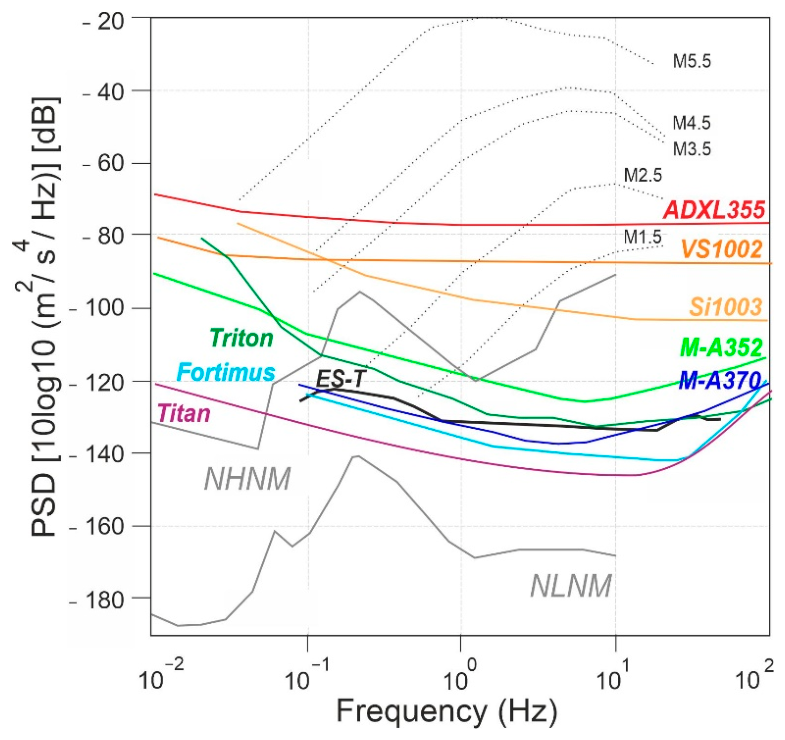
Figure 2.
Comparison of signal processing chains between a conventional capacitive MEMS accelerometer (a) and the QMEMS accelerometer (b). The QMEMS approach utilizes direct acceleration-to-frequency conversion and digital frequency measurement, avoiding the conventional analog amplification and voltage-based A/D conversion chain, thereby reducing the associated sources of noise and non-linearity.
Figure 2.
Comparison of signal processing chains between a conventional capacitive MEMS accelerometer (a) and the QMEMS accelerometer (b). The QMEMS approach utilizes direct acceleration-to-frequency conversion and digital frequency measurement, avoiding the conventional analog amplification and voltage-based A/D conversion chain, thereby reducing the associated sources of noise and non-linearity.
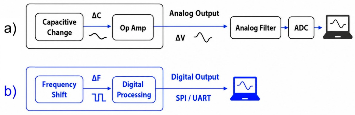
Figure 3.
a) External view of the M-A370 accelerometer module. The compact aluminum housing (48×24×16 mm³) contains the 3-axis sensor assembly and digital readout electronics, offering a significant size advantage for dense array deployments. b) Internal structure of the M-A370 sensor module. The exploded view (left) shows the differential arrangement of the six transducer units (two per axis) mounted within the package. The detailed schematic (top right) illustrates the high-density tungsten proof mass attached to the quartz cantilever and DETF resonator. The SEM image (bottom right) shows the fabricated Double-Ended Tuning Fork (DETF) resonator.
Figure 3.
a) External view of the M-A370 accelerometer module. The compact aluminum housing (48×24×16 mm³) contains the 3-axis sensor assembly and digital readout electronics, offering a significant size advantage for dense array deployments. b) Internal structure of the M-A370 sensor module. The exploded view (left) shows the differential arrangement of the six transducer units (two per axis) mounted within the package. The detailed schematic (top right) illustrates the high-density tungsten proof mass attached to the quartz cantilever and DETF resonator. The SEM image (bottom right) shows the fabricated Double-Ended Tuning Fork (DETF) resonator.
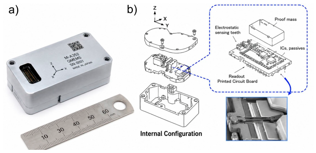
Figure 4.
Functional architecture of the multiparametric Smart Sensor Box used in this study. The system integrates a high-sensitivity Epson M-A352/M-A370 QMEMS accelerometer, a GNSS-disciplined Time Base Unit (TBU), a dual-core STM32H7 microcontroller, and an embedded single-board computer providing edge-computing capabilities. The modular architecture supports deterministic timing, local data processing, multi-parameter environmental sensing, and distributed communication through wired and wireless interfaces, providing a scalable framework for seismic monitoring and Structural Health Monitoring applications.
Figure 4.
Functional architecture of the multiparametric Smart Sensor Box used in this study. The system integrates a high-sensitivity Epson M-A352/M-A370 QMEMS accelerometer, a GNSS-disciplined Time Base Unit (TBU), a dual-core STM32H7 microcontroller, and an embedded single-board computer providing edge-computing capabilities. The modular architecture supports deterministic timing, local data processing, multi-parameter environmental sensing, and distributed communication through wired and wireless interfaces, providing a scalable framework for seismic monitoring and Structural Health Monitoring applications.
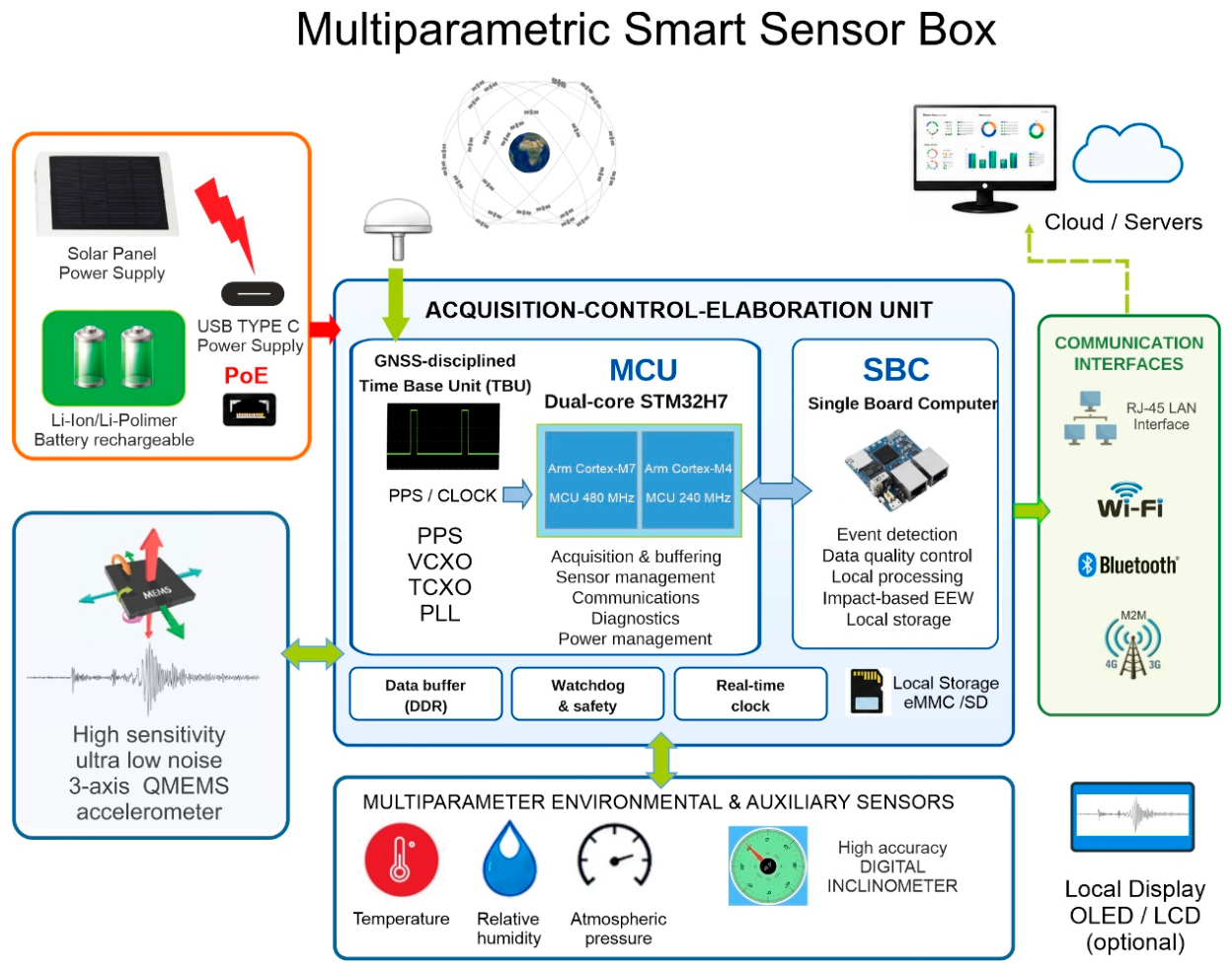
Figure 5.
Experimental setup adopted for the laboratory validation of the proposed QMEMS-based acquisition systems at the L.E.D.A. (Laboratory of Earthquake Engineering and Dynamic Analysis) Research Centre. (a) Complete Smart Sensor Box mounted on the SPEKTRA APS129 electrodynamic shaker for testing under the operational configuration. (b) Epson M-A352 and M-A370 QMEMS sensing elements mounted side-by-side on a rigid fixture for direct comparison of the sensor response independently of the enclosure. (c) Güralp Fortimus force-balance accelerometer installed on the shaker table a. (d) Frequency–amplitude excitation scheme adopted to evaluate sensor performance over the range of amplitudes and frequencies shown in panel.
Figure 5.
Experimental setup adopted for the laboratory validation of the proposed QMEMS-based acquisition systems at the L.E.D.A. (Laboratory of Earthquake Engineering and Dynamic Analysis) Research Centre. (a) Complete Smart Sensor Box mounted on the SPEKTRA APS129 electrodynamic shaker for testing under the operational configuration. (b) Epson M-A352 and M-A370 QMEMS sensing elements mounted side-by-side on a rigid fixture for direct comparison of the sensor response independently of the enclosure. (c) Güralp Fortimus force-balance accelerometer installed on the shaker table a. (d) Frequency–amplitude excitation scheme adopted to evaluate sensor performance over the range of amplitudes and frequencies shown in panel.
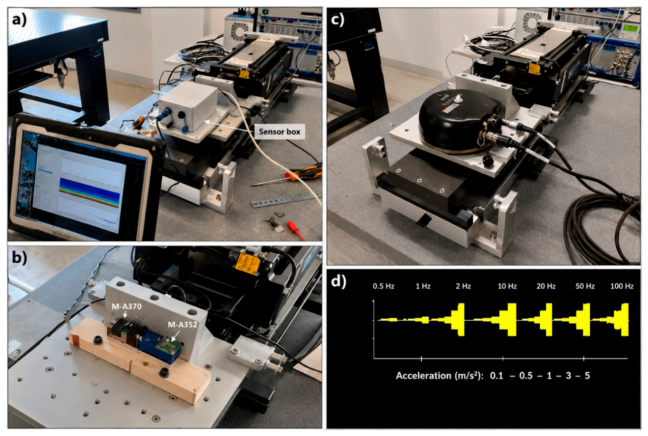
Figure 6.
Measured relative amplitude error as a function of excitation frequency for the three configurations: (a) Sensor Box integrating the Epson M-A370 QMEMS (b) standalone Epson M-A370 QMEMS accelerometer mounted directly on the shake table and (c) Güralp Fortimus force-balance accelerometer. The curves correspond to sinusoidal excitation tests performed at nominal peak acceleration amplitudes of 0.1, 0.5, 1, 3, and 5 m s⁻².
Figure 6.
Measured relative amplitude error as a function of excitation frequency for the three configurations: (a) Sensor Box integrating the Epson M-A370 QMEMS (b) standalone Epson M-A370 QMEMS accelerometer mounted directly on the shake table and (c) Güralp Fortimus force-balance accelerometer. The curves correspond to sinusoidal excitation tests performed at nominal peak acceleration amplitudes of 0.1, 0.5, 1, 3, and 5 m s⁻².
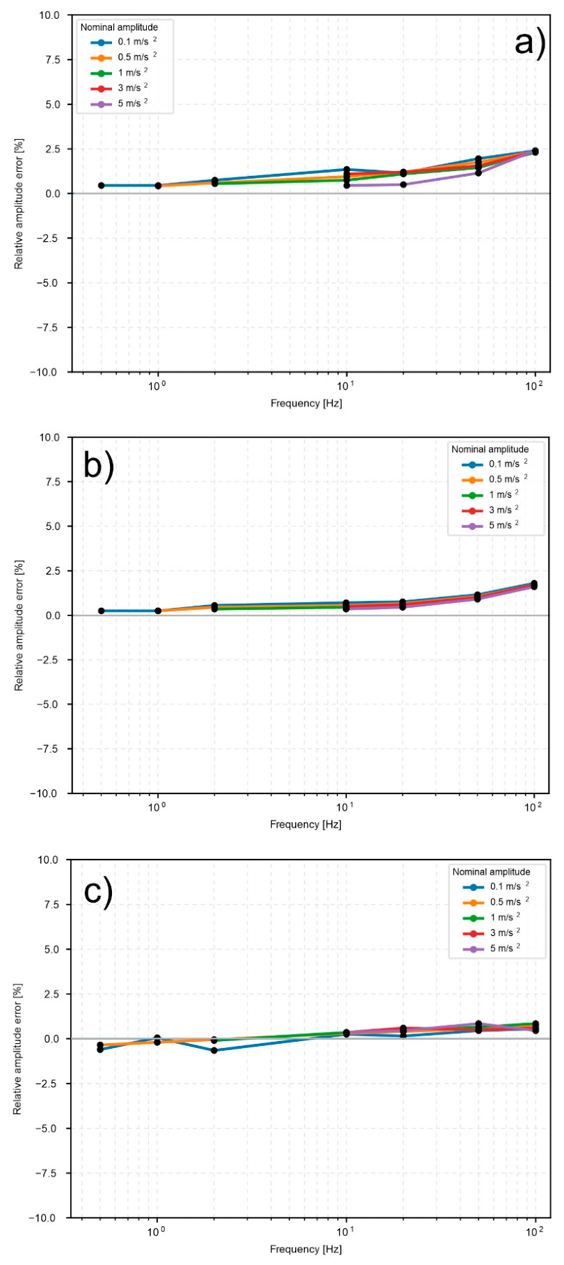
Figure 7.
Experimental setup and representative stabilization diagrams obtained during the dynamic testing campaign on the 2:3 scale masonry building at the L.E.D.A. laboratory (modified from [41]. The comparison among the M-A352 (a), PCB 356A17 (b), VS1002 (c), and ADXL355 (d) sensors highlights the influence of their self-noise on the identification of structural modal frequencies under ambient-vibration conditions, with the M-A352 and PCB 356A17 providing the clearest stabilization diagrams.
Figure 7.
Experimental setup and representative stabilization diagrams obtained during the dynamic testing campaign on the 2:3 scale masonry building at the L.E.D.A. laboratory (modified from [41]. The comparison among the M-A352 (a), PCB 356A17 (b), VS1002 (c), and ADXL355 (d) sensors highlights the influence of their self-noise on the identification of structural modal frequencies under ambient-vibration conditions, with the M-A352 and PCB 356A17 providing the clearest stabilization diagrams.
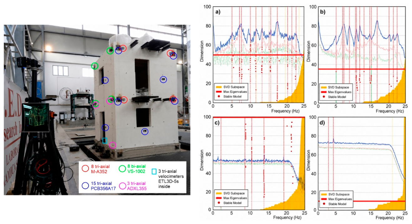
Figure 8.
Relative timing drift between the GNSS-derived PPS and the synthetic PPS during holdover operation. The reported values represent the measured timing difference between the GNSS-derived PPS and the synthetic PPS generated by the TBU as a function of elapsed time after GNSS disconnection. The timing offset was determined from direct oscilloscope measurements of the temporal separation between the rising edges of the two PPS signals. During the approximately 4.4 h experiment, the relative timing error remained within ± 80 μs.
Figure 8.
Relative timing drift between the GNSS-derived PPS and the synthetic PPS during holdover operation. The reported values represent the measured timing difference between the GNSS-derived PPS and the synthetic PPS generated by the TBU as a function of elapsed time after GNSS disconnection. The timing offset was determined from direct oscilloscope measurements of the temporal separation between the rising edges of the two PPS signals. During the approximately 4.4 h experiment, the relative timing error remained within ± 80 μs.
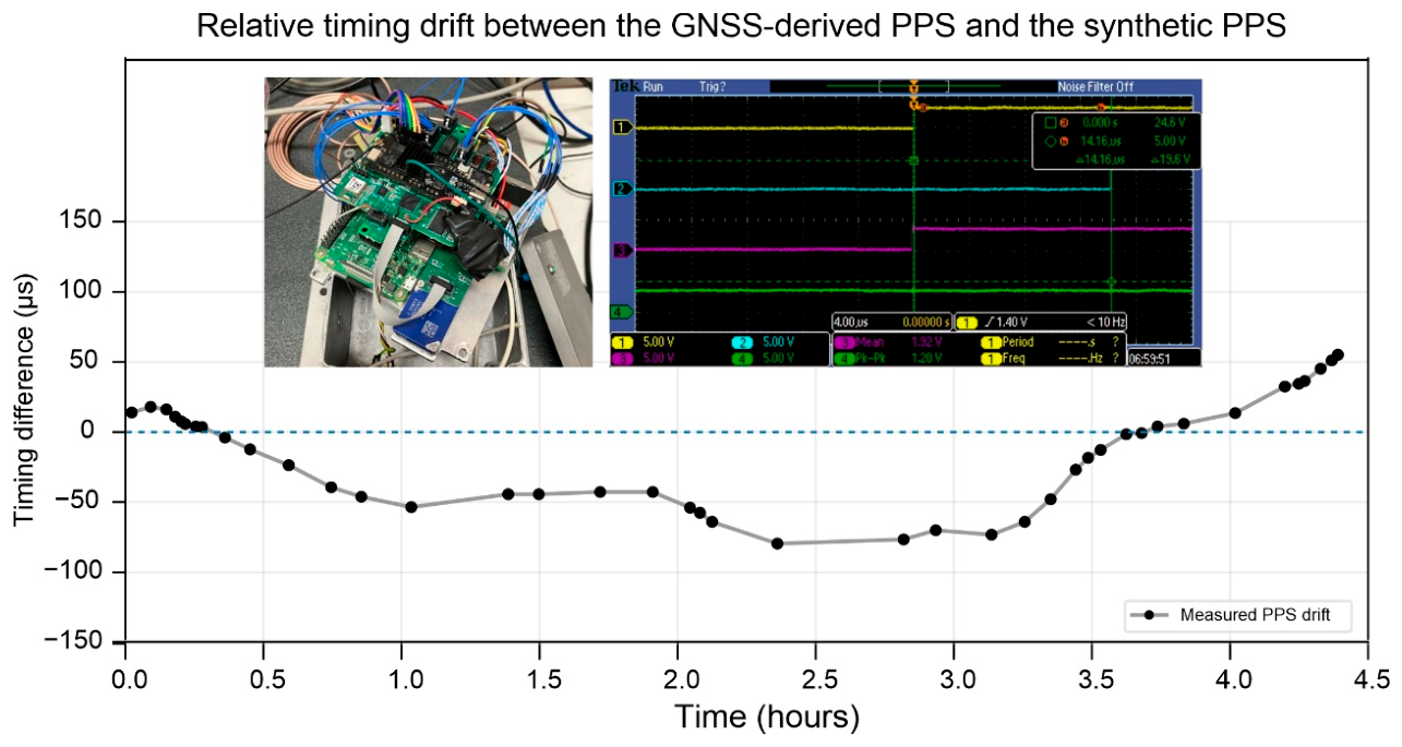
Figure 9.
Example of synchronization validation between two co-located Smart Sensor Boxes (CT02 and CT04) operating under GNSS-disciplined timing and sampling simultaneously at 1000 Hz. The upper panels compare the recorded N–S acceleration waveforms and their Power Spectral Density (PSD), showing an excellent agreement in both the time and frequency domains. The central panels report the global coherence and phase difference between the two signals, demonstrating coherence values close to unity and negligible phase shifts across the frequency band of interest. The lower panels show the evolution of coherence and cross-correlation within selected frequency bands (0.5–5 Hz, 5–10 Hz, and 10–30 Hz), confirming the stability of the synchronization throughout the entire recording. Sub-sample cross-correlation analysis yields a residual relative timing offset of only 0.009 samples, corresponding to approximately 9.1 μs, with a correlation coefficient equal to 1.0 and an equivalent phase difference of only 0.02° at 5 Hz.
Figure 9.
Example of synchronization validation between two co-located Smart Sensor Boxes (CT02 and CT04) operating under GNSS-disciplined timing and sampling simultaneously at 1000 Hz. The upper panels compare the recorded N–S acceleration waveforms and their Power Spectral Density (PSD), showing an excellent agreement in both the time and frequency domains. The central panels report the global coherence and phase difference between the two signals, demonstrating coherence values close to unity and negligible phase shifts across the frequency band of interest. The lower panels show the evolution of coherence and cross-correlation within selected frequency bands (0.5–5 Hz, 5–10 Hz, and 10–30 Hz), confirming the stability of the synchronization throughout the entire recording. Sub-sample cross-correlation analysis yields a residual relative timing offset of only 0.009 samples, corresponding to approximately 9.1 μs, with a correlation coefficient equal to 1.0 and an equivalent phase difference of only 0.02° at 5 Hz.
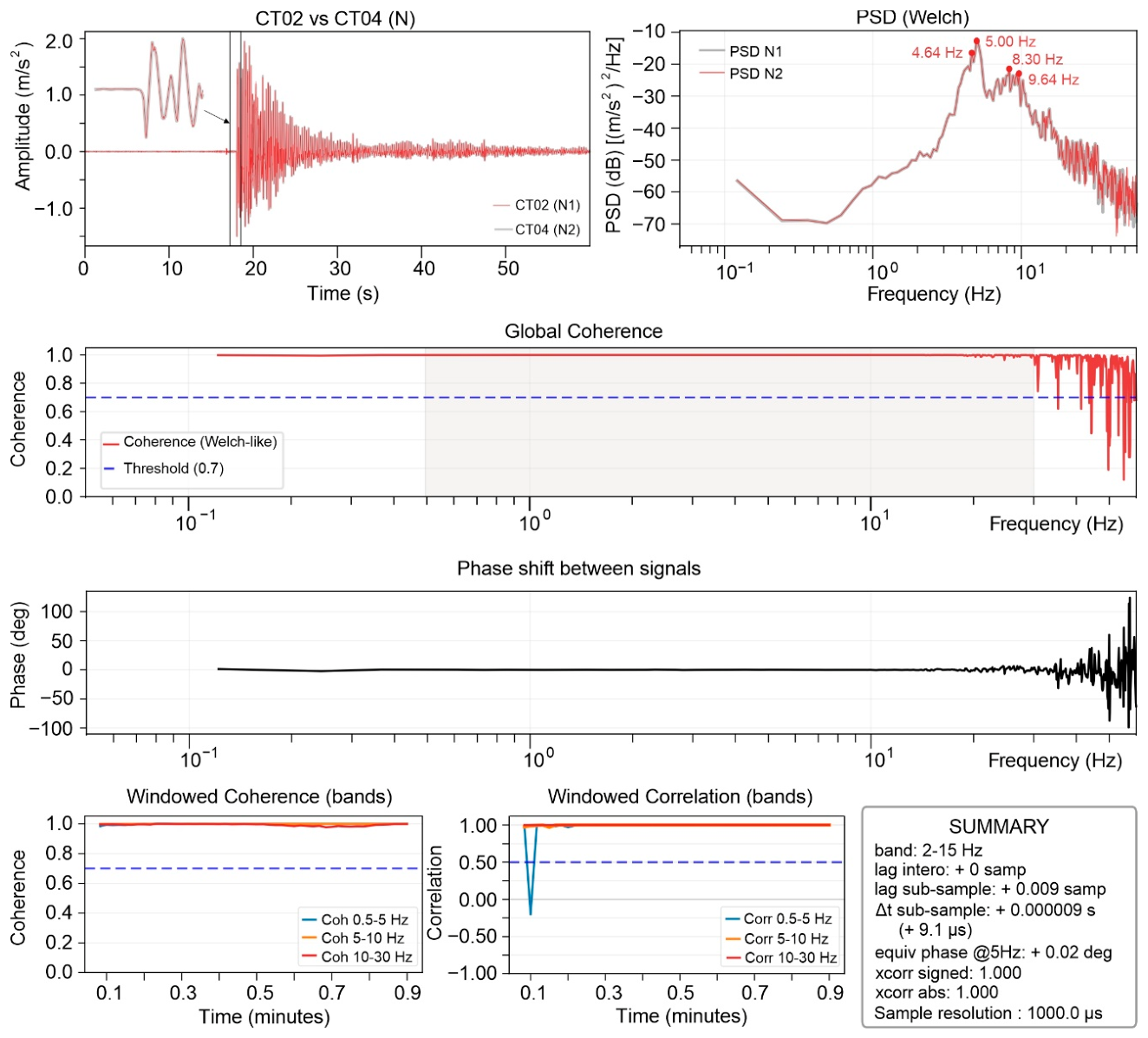
Figure 10.
Drift rate of the CT02–CT04 timing offset during GNSS holdover operation and comparison with the external ambient temperature measured by the BME280 sensor. The left axis shows the first derivative of the timing drift (μs h⁻¹), whereas the right axis reports the corresponding temperature evolution. Labels indicate the cumulative timing drift (ms) measured at each epoch.
Figure 10.
Drift rate of the CT02–CT04 timing offset during GNSS holdover operation and comparison with the external ambient temperature measured by the BME280 sensor. The left axis shows the first derivative of the timing drift (μs h⁻¹), whereas the right axis reports the corresponding temperature evolution. Labels indicate the cumulative timing drift (ms) measured at each epoch.
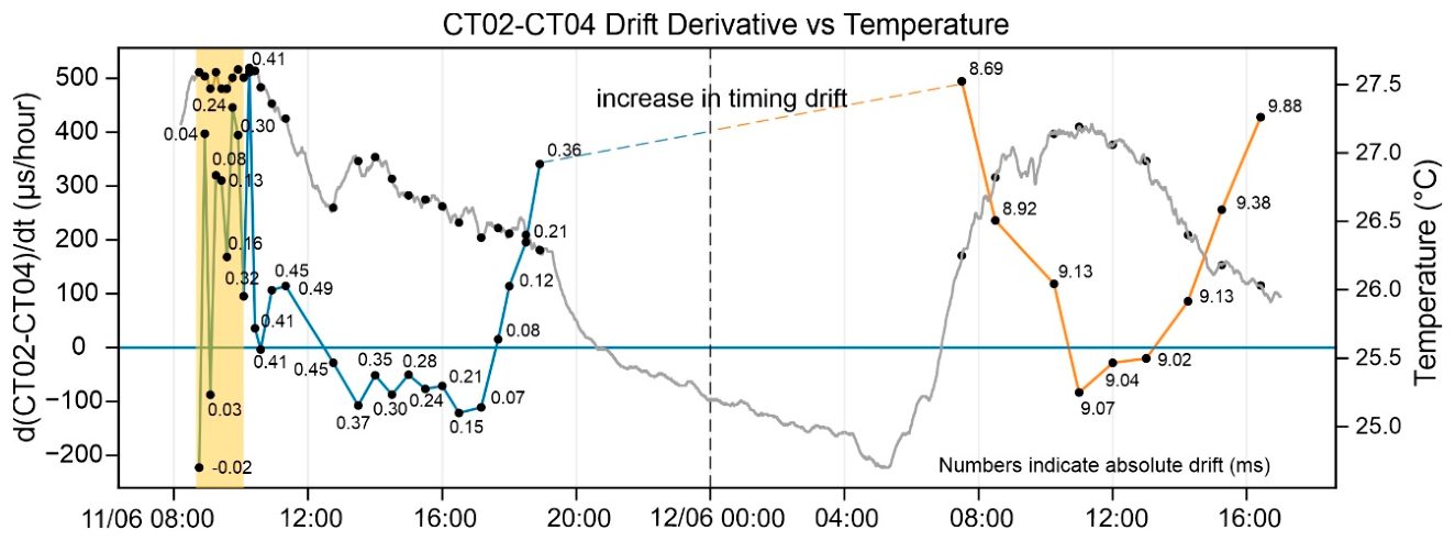
Figure 11.
Southern Italy map with the spatial distribution of the urban seismic observatories of CMSU. Colored squares indicate the epicenters of historical earthquakes with magnitude larger than 5.5. In the insets are shown the investigated areas together with the station distribution (yellow triangles) within the urban environments of Catania, Campi Flegrei, Messina–Reggio Calabria, Potenza, port of Vulcano, and Ragusa. In Catania, Potenza, and Ragusa, QMEMS sensors are integrated with force-balance and conventional MEMS accelerometers, whereas only QMEMS deployments are represented for the Messina–Reggio Calabria and Campi Flegrei volcanic area, where more than 50 QMEMS M-A352 accelerometer are currently in operation.
Figure 11.
Southern Italy map with the spatial distribution of the urban seismic observatories of CMSU. Colored squares indicate the epicenters of historical earthquakes with magnitude larger than 5.5. In the insets are shown the investigated areas together with the station distribution (yellow triangles) within the urban environments of Catania, Campi Flegrei, Messina–Reggio Calabria, Potenza, port of Vulcano, and Ragusa. In Catania, Potenza, and Ragusa, QMEMS sensors are integrated with force-balance and conventional MEMS accelerometers, whereas only QMEMS deployments are represented for the Messina–Reggio Calabria and Campi Flegrei volcanic area, where more than 50 QMEMS M-A352 accelerometer are currently in operation.
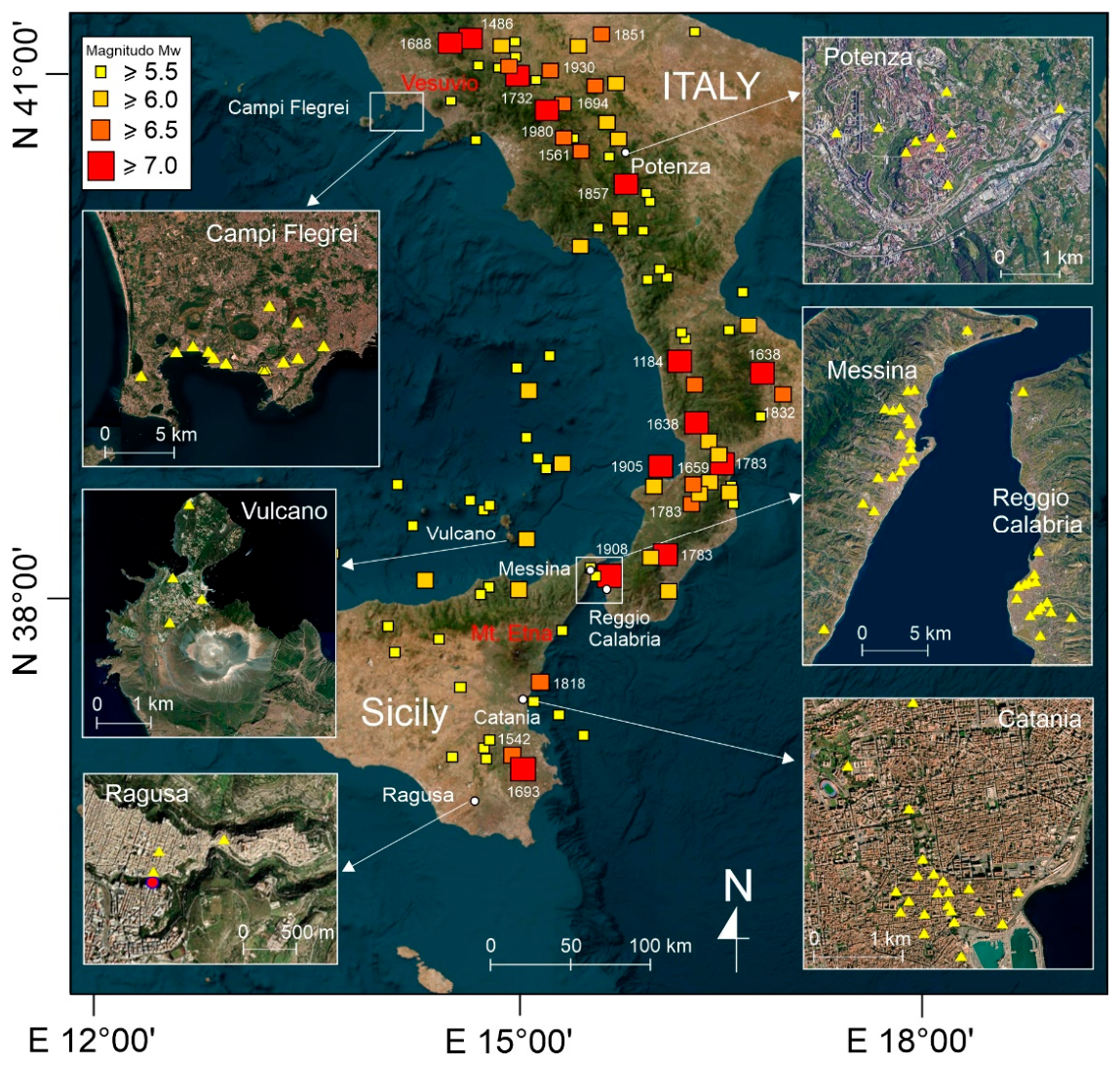
Figure 12.
Example of continuous seismic recordings acquired at station OCF04 of the Campi Flegrei Urban Seismic Observatory using an Epson M-A352 QMEMS accelerometer. The left panel shows a continuous record collected on 1 September 2025, including the Md 4.0 earthquake together with several smaller local events. The panel on the right illustrates the three-component recording of a Md 1.0 earthquake, highlighting the capability of the QMEMS sensor to detect and accurately record very weak local seismic events.
Figure 12.
Example of continuous seismic recordings acquired at station OCF04 of the Campi Flegrei Urban Seismic Observatory using an Epson M-A352 QMEMS accelerometer. The left panel shows a continuous record collected on 1 September 2025, including the Md 4.0 earthquake together with several smaller local events. The panel on the right illustrates the three-component recording of a Md 1.0 earthquake, highlighting the capability of the QMEMS sensor to detect and accurately record very weak local seismic events.
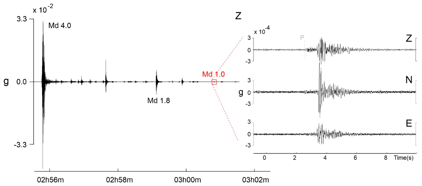
Figure 13.
Response of the Messina–Reggio Calabria Urban Seismic Observatory (OSU) stations to the deep Mw 6.1 earthquake of 1 June 2026. (a) Overview of the event, showing the vertical (Z) component waveforms recorded at twenty OSU stations, the corresponding regional INGV ShakeMap (https://shakemap.ingv.it/data/46107472/current/products/pga.jpg), and the geographical distribution of the stations across the Messina Strait. (b) Spatial distribution of the maximum PGV and PGA values. For each station, the reported values correspond to the maximum among the three components (Z, N, and E). Circle size and colour are proportional to the measured amplitudes, while the numerical labels indicate the corresponding PGV (cm s⁻¹) and PGA (% g) values.
Figure 13.
Response of the Messina–Reggio Calabria Urban Seismic Observatory (OSU) stations to the deep Mw 6.1 earthquake of 1 June 2026. (a) Overview of the event, showing the vertical (Z) component waveforms recorded at twenty OSU stations, the corresponding regional INGV ShakeMap (https://shakemap.ingv.it/data/46107472/current/products/pga.jpg), and the geographical distribution of the stations across the Messina Strait. (b) Spatial distribution of the maximum PGV and PGA values. For each station, the reported values correspond to the maximum among the three components (Z, N, and E). Circle size and colour are proportional to the measured amplitudes, while the numerical labels indicate the corresponding PGV (cm s⁻¹) and PGA (% g) values.
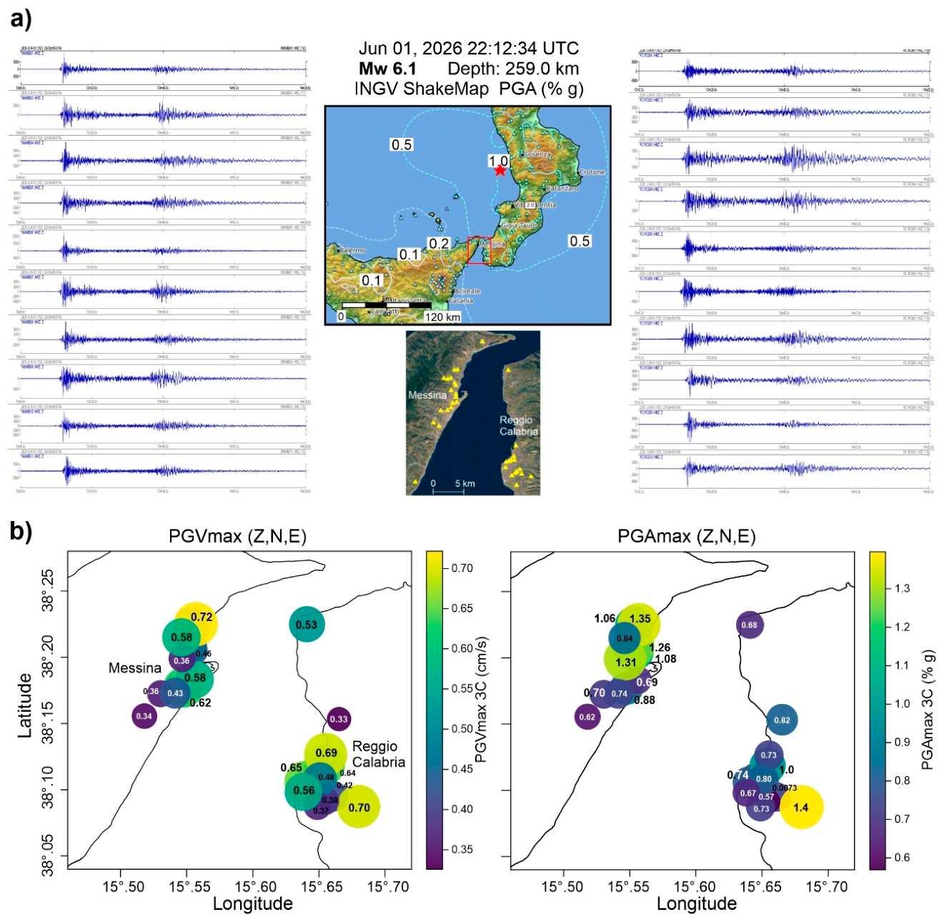
Figure 14.
Example of the products generated by PSAVE at the ME016 station of Messina network during the the Mw 6.1 earthquake of 1 June 2026 (22:12:35 UTC), which occurred at a hypocentral depth of approximately 250 km from Messina–Reggio Calabria Urban Seismic Observatory networks for. (a) PSAVE impact-based EEW summary showing both predictive and observed parameters; (b) pseudo-spectral acceleration curves and three-component acceleration time histories.
Figure 14.
Example of the products generated by PSAVE at the ME016 station of Messina network during the the Mw 6.1 earthquake of 1 June 2026 (22:12:35 UTC), which occurred at a hypocentral depth of approximately 250 km from Messina–Reggio Calabria Urban Seismic Observatory networks for. (a) PSAVE impact-based EEW summary showing both predictive and observed parameters; (b) pseudo-spectral acceleration curves and three-component acceleration time histories.
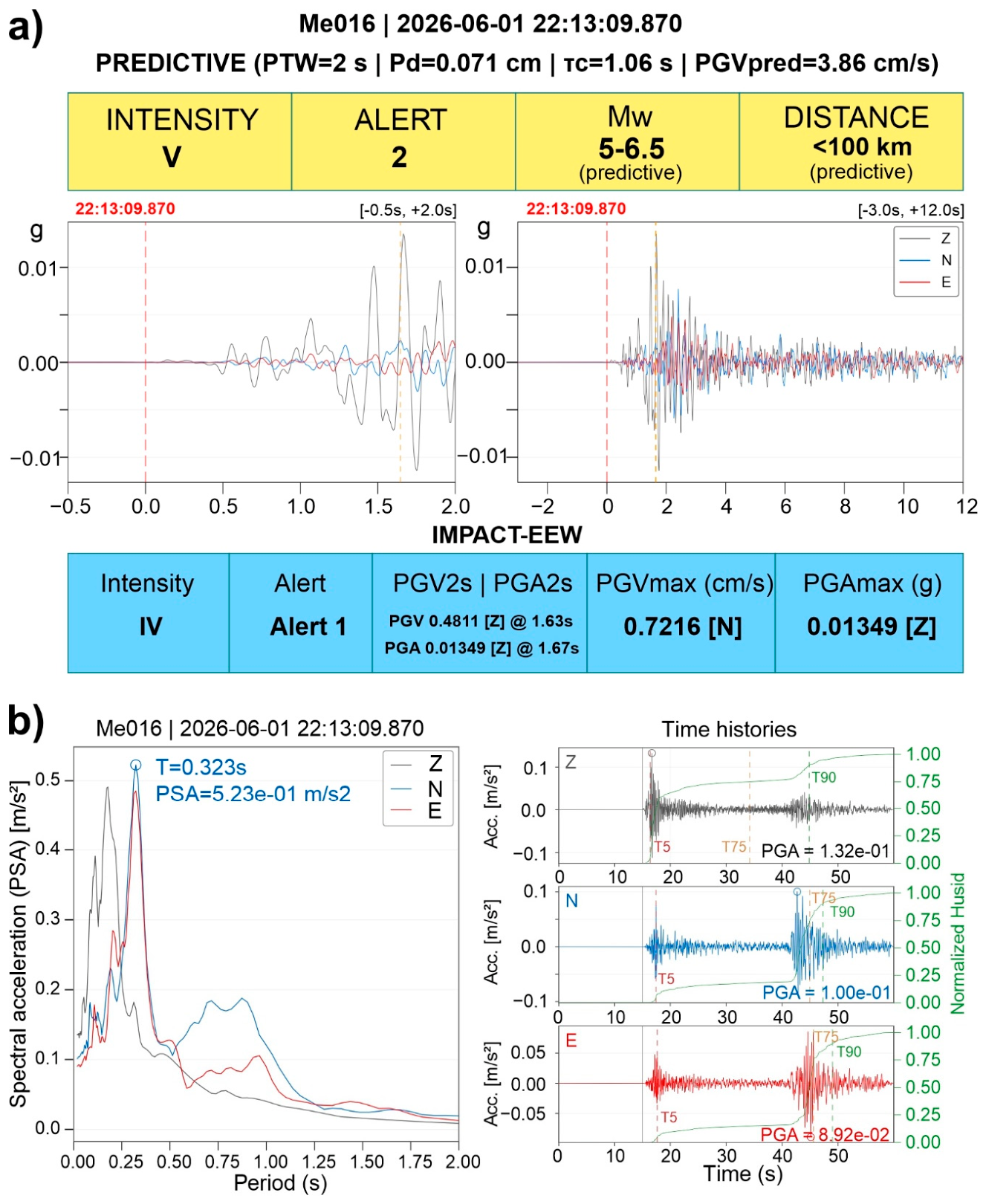
Figure 15.
Adopted sensor layout at the clock tower during the ambient vibration campaign. M-A352 accelerometers were installed at the ground floor and at the clock level of the tower.
Figure 15.
Adopted sensor layout at the clock tower during the ambient vibration campaign. M-A352 accelerometers were installed at the ground floor and at the clock level of the tower.
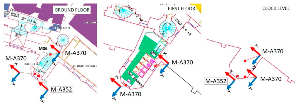
Figure 16.
Experimental setup and comparison of the self-noise characteristics of the M-A352 and M-A370 accelerometers at the clock tower of the Durham Castle (United Kingdom). Power spectral densities (PSDs) calculated from one hour (01:00–02:00 UTC) of ambient-noise recordings acquired simultaneously by co-located sensors installed at the top and base of the Clock Tower reveal several structural resonance frequencies between 2 and 10 Hz, with larger amplification observed at the top of the structure.
Figure 16.
Experimental setup and comparison of the self-noise characteristics of the M-A352 and M-A370 accelerometers at the clock tower of the Durham Castle (United Kingdom). Power spectral densities (PSDs) calculated from one hour (01:00–02:00 UTC) of ambient-noise recordings acquired simultaneously by co-located sensors installed at the top and base of the Clock Tower reveal several structural resonance frequencies between 2 and 10 Hz, with larger amplification observed at the top of the structure.
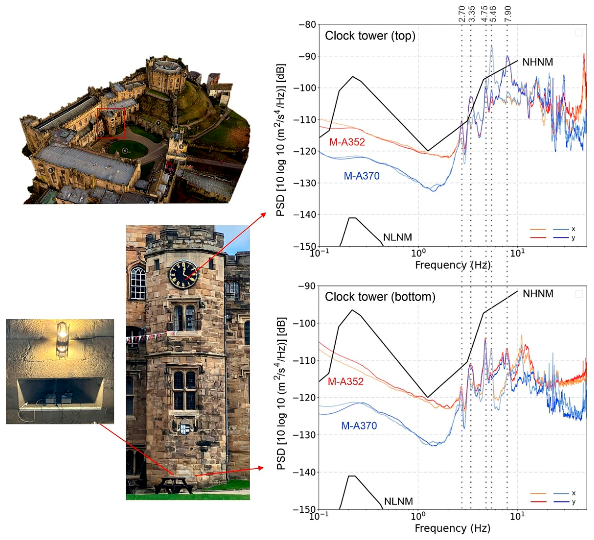
Figure 17.
Structural Health Monitoring of the “Papa Giovanni XXIII” reinforced-concrete arch bridge in Ragusa (southern Italy). (a) General view of the bridge. (b) Stabilization diagram obtained from Operational Modal Analysis (OMA) during the dynamic characterization together with the corresponding first bending mode shape identified at 1.61 Hz. (c) Comparison of power spectral densities computed from one hour of nighttime ambient-vibration recordings acquired by co-located ADXL355 and M-A352 accelerometers, highlighting the lower self-noise and improved detectability of structural resonances provided by the M-A352 sensor. (d) Automatic tracking of the first five modal frequencies over several months for the three components at a representative monitoring node.
Figure 17.
Structural Health Monitoring of the “Papa Giovanni XXIII” reinforced-concrete arch bridge in Ragusa (southern Italy). (a) General view of the bridge. (b) Stabilization diagram obtained from Operational Modal Analysis (OMA) during the dynamic characterization together with the corresponding first bending mode shape identified at 1.61 Hz. (c) Comparison of power spectral densities computed from one hour of nighttime ambient-vibration recordings acquired by co-located ADXL355 and M-A352 accelerometers, highlighting the lower self-noise and improved detectability of structural resonances provided by the M-A352 sensor. (d) Automatic tracking of the first five modal frequencies over several months for the three components at a representative monitoring node.
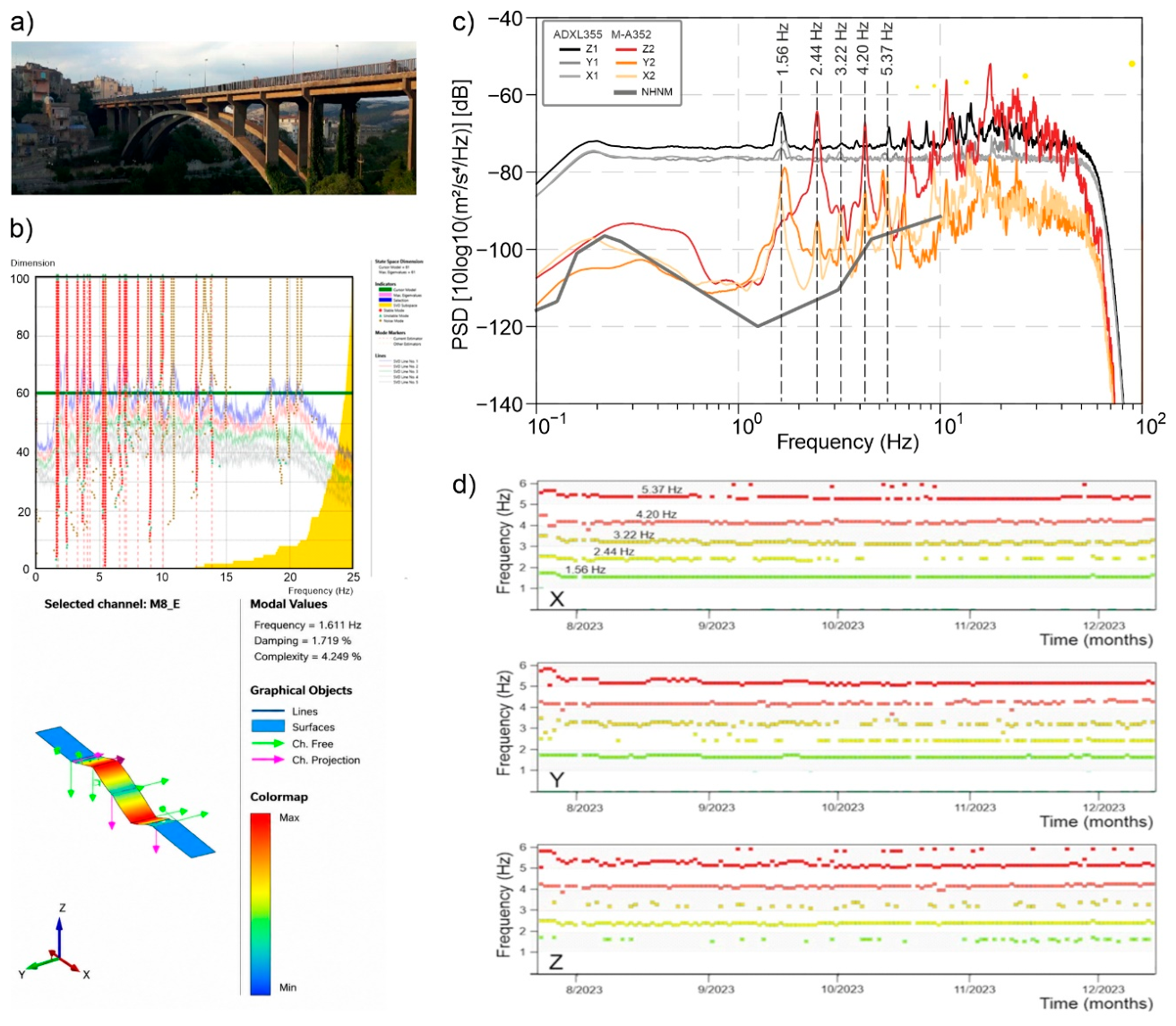
Figure 18.
Instrumented buildings ED001–ED003 and corresponding stabilization diagrams derived from ambient vibration measurements through the SSI-Data method. Stable poles indicate the identified modal frequencies, revealing two flexural modes and one torsional mode for each structure.
Figure 18.
Instrumented buildings ED001–ED003 and corresponding stabilization diagrams derived from ambient vibration measurements through the SSI-Data method. Stable poles indicate the identified modal frequencies, revealing two flexural modes and one torsional mode for each structure.
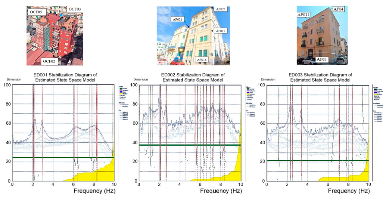
Figure 19.
Pseudo-acceleration response spectra and three-component acceleration time histories of the Md 4.4 earthquake of 20 May 2024 recorded at stations OCF03 (top panels, basement level) and OCF02 (bottom panels, rooftop level) installed in building ED001 (see Figure 18). The Husid plot (green line), representing the cumulative energy release of the signal, is superimposed on the time histories and was used to estimate the significant durations T75 and T90, whose values are indicated by the red arrows. Comparison between the basement and rooftop recordings highlights the amplification effects associated with the dynamic response of the structure.
Figure 19.
Pseudo-acceleration response spectra and three-component acceleration time histories of the Md 4.4 earthquake of 20 May 2024 recorded at stations OCF03 (top panels, basement level) and OCF02 (bottom panels, rooftop level) installed in building ED001 (see Figure 18). The Husid plot (green line), representing the cumulative energy release of the signal, is superimposed on the time histories and was used to estimate the significant durations T75 and T90, whose values are indicated by the red arrows. Comparison between the basement and rooftop recordings highlights the amplification effects associated with the dynamic response of the structure.
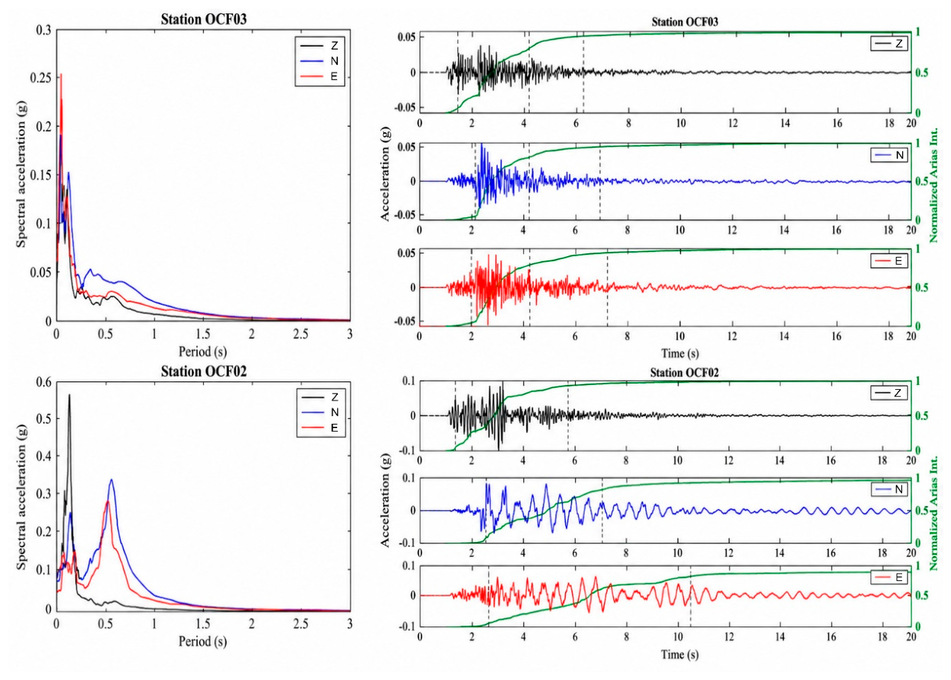
Figure 20.
Automatic tracking of the modal frequencies of building ED001 derived from power spectral density (PSD) analysis during the Md 3.5 and Md 4.4 earthquakes of 20 May 2024. The upper panel shows the vertical acceleration record (HNZ), while the lower panels display the evolution of the spectral peaks identified on the three components (HNZ, HNN, and HNE). Zoomed views (right panels) highlight the temporary decrease of the first modal frequency during the Md 4.4 earthquake and its subsequent recovery; a similar but less pronounced behavior was previously observed during the preceding Md 3.5 event. The conceptual sketch illustrates the temporary reduction of structural stiffness during shaking, associated with soil–structure interaction and nonlinear structural behavior, and the subsequent recovery of the original dynamic properties after the event, indicating the absence of permanent damage.
Figure 20.
Automatic tracking of the modal frequencies of building ED001 derived from power spectral density (PSD) analysis during the Md 3.5 and Md 4.4 earthquakes of 20 May 2024. The upper panel shows the vertical acceleration record (HNZ), while the lower panels display the evolution of the spectral peaks identified on the three components (HNZ, HNN, and HNE). Zoomed views (right panels) highlight the temporary decrease of the first modal frequency during the Md 4.4 earthquake and its subsequent recovery; a similar but less pronounced behavior was previously observed during the preceding Md 3.5 event. The conceptual sketch illustrates the temporary reduction of structural stiffness during shaking, associated with soil–structure interaction and nonlinear structural behavior, and the subsequent recovery of the original dynamic properties after the event, indicating the absence of permanent damage.
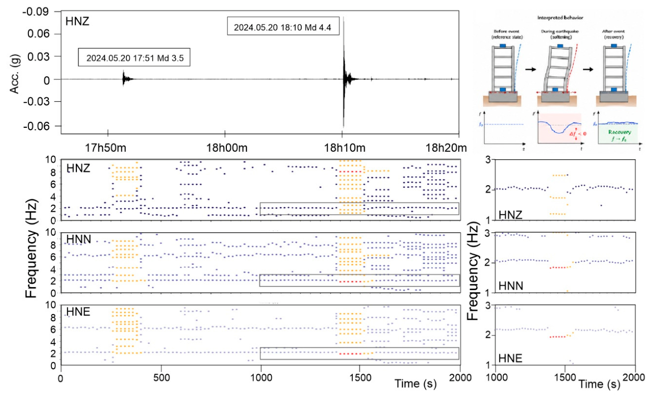

Table 1.
Comparison of representative force-balance (FBA), MEMS and QMEMS accelerometers for seismic monitoring and Structural Health Monitoring (SHM) applications. Most of the listed sensors were employed in the experimental activities presented in this work. Specifications are taken from the corresponding manufacturers’ datasheets.
Table 1.
Comparison of representative force-balance (FBA), MEMS and QMEMS accelerometers for seismic monitoring and Structural Health Monitoring (SHM) applications. Most of the listed sensors were employed in the experimental activities presented in this work. Specifications are taken from the corresponding manufacturers’ datasheets.
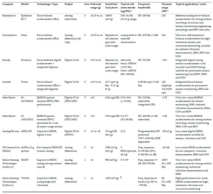 |
* Noise values are reported according to the quantities specified by each manufacturer (spectral noise density, RMS noise, or equivalent performance relative to NHNM/AHNM), and therefore should not be interpreted as directly comparable. ** Dynamic range values are those specified by the manufacturers. The achievable system dynamic range depends on the complete acquisition chain, including sensor configuration, signal conditioning, digitizer (ADC) resolution, and processing electronics.
Table 2.
Comparison of representative IEPE (ICP®) accelerometers commonly used for structural dynamics and laboratory testing. Most of the listed sensors were employed in the experimental activities presented in this work. Specifications are taken from the corresponding manufacturers’ datasheets; dynamic range values marked with (*) were estimated as described in the text.
Table 2.
Comparison of representative IEPE (ICP®) accelerometers commonly used for structural dynamics and laboratory testing. Most of the listed sensors were employed in the experimental activities presented in this work. Specifications are taken from the corresponding manufacturers’ datasheets; dynamic range values marked with (*) were estimated as described in the text.
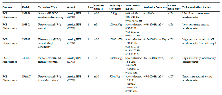 |
* Dynamic range values marked with (*) were estimated from the manufacturer’s specifications over the 0.5–30 Hz bandwidth, assuming white noise equal to the spectral noise density specified at 10 Hz and a full-scale sinusoidal RMS amplitude (FS/√2). However, the actual dynamic range depends on the complete acquisition chain, including IEPE signal conditioning and ADC resolution.
Table 3.
Typical synchronization requirements for seismic monitoring, Operational Modal Analysis (OMA), and Structural Health Monitoring (SHM) applications.
Table 3.
Typical synchronization requirements for seismic monitoring, Operational Modal Analysis (OMA), and Structural Health Monitoring (SHM) applications.
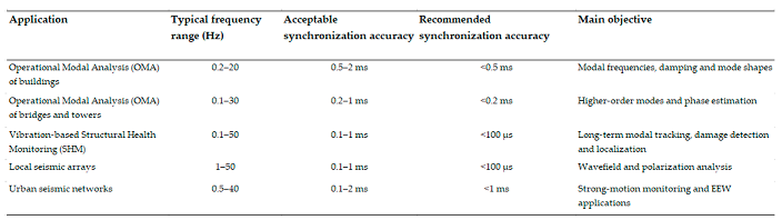 |
Table 4.
Measured synchronization performance of the system investigated in this study.
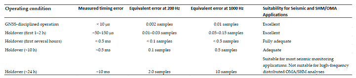 |
Table 5.
Modal parameters identified by Operational Modal Analysis for the first three monitored buildings (ED001–ED003), including modal frequency, damping ratio, and complexity index.
Table 5.
Modal parameters identified by Operational Modal Analysis for the first three monitored buildings (ED001–ED003), including modal frequency, damping ratio, and complexity index.
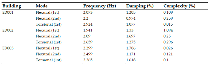 |
Table 6.
Indicative engineering guidelines relating accelerometer self-noise and timing synchronization requirements for seismic monitoring, Operational Modal Analysis (OMA), and Structural Health Monitoring (SHM) applications. The reported values represent indicative performance ranges derived from laboratory experiments, field deployments, and representative applications discussed in this work, complemented by evidence from the literature. They should not be interpreted as strict thresholds, since actual requirements depend on the monitored structure, ambient vibration levels, monitoring objectives, and the target application.
Table 6.
Indicative engineering guidelines relating accelerometer self-noise and timing synchronization requirements for seismic monitoring, Operational Modal Analysis (OMA), and Structural Health Monitoring (SHM) applications. The reported values represent indicative performance ranges derived from laboratory experiments, field deployments, and representative applications discussed in this work, complemented by evidence from the literature. They should not be interpreted as strict thresholds, since actual requirements depend on the monitored structure, ambient vibration levels, monitoring objectives, and the target application.
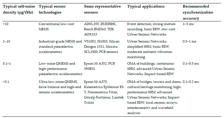 |
Note: Self-noise values are indicative and represent typical performance ranges reported by manufacturers and experimental studies. Since self-noise is frequency dependent, these values should be regarded as representative rather than frequency-specific. Actual performance may vary with sensor technology, operating conditions, and the frequency range of interest.
Disclaimer/Publisher’s Note: The statements, opinions and data contained in all publications are solely those of the individual author(s) and contributor(s) and not of MDPI and/or the editor(s). MDPI and/or the editor(s) disclaim responsibility for any injury to people or property resulting from any ideas, methods, instructions or products referred to in the content. |
© 2026 by the authors. Licensee MDPI, Basel, Switzerland. This article is an open access article distributed under the terms and conditions of the Creative Commons Attribution (CC BY) license (http://creativecommons.org/licenses/by/4.0/).
Copyright: This open access article is published under a Creative Commons CC BY 4.0 license, which permit the free download, distribution, and reuse, provided that the author and preprint are cited in any reuse.


