

Submitted:
07 July 2026
Posted:
08 July 2026
You are already at the latest version
Abstract
This article proposed to amend the Chu formulation Maxwell’s equations for moving media. The Fresnel’s coefficient is correctly derived from the classical electromagnetic theory. The Maxwell’s equations for moving media are theoretical bases for analyzing the electromagnetic scattering properties of moving media. However, the magnetization effect due to moving electric dipoles has not been taken into account in the formulations, and the Frensel’s dragging coefficient cannot be correctly derived from them. These inconsistencies have cast a shadow on their applications in the analysis of scattering problems involving fast-moving media. The method in modeling a moving Hertzian dipole and that in modelling the polarization in a moving medium are compared. The plane wave solutions for the Maxwell’s equations in uniformly moving media are used for deriving the Fresnel’s coefficient. The results show that the two inconsistencies are closely related and can be removed together if the Chu formulation Maxwell’s equations for moving media are amended by taking into account the magnetization effect.
Keywords:
Fresnel’s coefficient
; Chu formulation
; moving media
; Maxwell’s equations
1. Introduction
The classical electromagnetic theory is one of the most successful theories in history, in which the Maxwell’s equations play a central role [1,2,3]. However, there still exist a few inconsistencies or even controversies in it, especially concerning with the electrodynamics of moving objects and moving media [4].
There are several formulations of Maxwell’s equations for moving media. We take the Chu formulation [4,5,6,7] as an example to show the inconsistencies. When being exposed in an external electric field, the molecules or atoms in the medium will be polarized. In simple substances, the dominant molecule moment is the dipole and the polarization can be characterized with electric dipoles. We usually utilize the polarization vector to represent the volume density of the electric dipoles. The electric polarization current and the electric polarization charge can be expressed in terms of the polarization vector with and . When the medium moves with velocity , the derivative terms with respect to time should be replaced by the corresponding substantial derivatives [8]. The continuity law for the polarization current is derived to be
The terms in the square bracket amount to the electric polarization current in the moving medium, including an additional current produced by the moving polarization charge. For the sake of simplicity, we still denote it as , which can be transformed as follows,
On the other hand, when a medium is exposed in an external magnetic field, the magnetization will generate magnetic dipoles in the medium. The volume density of the magnetic dipoles is represented by the magnetization vector . The Lorentz model is used in Chu formulation [5,7], where a magnetic dipole is modelled with two closely located magnetic charges , and are connected with a magnetic current . In the symbols for current and charge, we use the superscript to indicate whether they are electric quantities or magnetic quantities, and the subscript to indicate whether they are caused by polarization or by magnetization.
The Chu formulation Maxwell’s equations for moving media [4] are summarized as follows
where and are the current density and charge density associated with free charges.
However, Chu formulation (3) is not in compatible with the Fresnel’s coefficient. Fresnel proposed in 1818 the famous Fresnel coefficient [9,10,11] when he attempted to explain the Arago’s experiments. His theory is based on a stationary ether. The light speed in a medium is , where is the light speed in the vacuum and is the refractive index of the medium at rest. When the medium moves with velocity , the light may be dragged by the medium and the light speed in the moving medium must change. If we determine the light speed according to the Newtonian mechanics, the two velocities should be added like vectors, namely, , in which it takes positive sign when the light propagates in the same direction with the medium and negative when in the opposite direction. However, this prediction was found to be not in agreement with the experimental results. Therefore, Fresnel assumed that when a medium moves through the stationary ether, it only drags the light propagating through it with a fraction of the medium’s speed, that is, the light speed in the moving medium is of the form
where is the Fresnel’s dragging coefficient.
We are now to find the plane wave solution of (3) in a uniformly moving homogeneous nonmagnetic medium like water. In this situation, we have , , and in the medium. Assume that the plane wave propagates in parallel with the moving direction of the medium and its fields take the form of , . From the two curl equations in (3) we obtain the matrix equation
The condition for (5) to have non-zero solutions is that its determinant vanishes, that is,
Solving from (6), we get
The corresponding solutions represent two plane waves propagating in the directions. Taking the plane wave in direction () as example, we obtain its phase velocity as below
where is the refractive index of the nonmagnetic medium. Obviously, the dragging coefficient in (8) is different from the Fresnel’s dragging coefficient in (4) by a factor of 0.5.
2. The Inconsistency with the Fields of a Moving Oscillating Dipole
A moving oscillating dipole can be modelled in two ways. The first one is to take the Lorentz model, in which the dipole is modelled with two closely-located charges with densities of , where is the small spacing between the two charges, is the unit vector of the electric polarization that points from to , and denotes the position of the center of the dipole on the trajectory. When , the two charge densities can be expressed concisely with
where is the electric dipole moment. According to the current continuity law, a short current filament with density of exists between the two charges. Besides this current, the moving charges also produce a current with density of
where is the velocity of the dipole. We use dot on top of a quantity to represent the derivative with respect to time . The total current density is the sum of the two currents,
The second method for modelling the dipole is based on the polarization vector , like that in handling moving media. For the oscillating moving dipole, we may consider that it is the polarization vector that is moving. Therefore, we can express the polarization vector by . The charge density expressed in terms of is the same as that has been defined previously.
The current density of the moving dipole expressed in term of consists of two terms,
Obviously, . Since represents the total current generated by the moving current filament and the current induced by the two moving charges, it is basically correct because its physical meaning is clear and intuitive. However, is derived from the electric polarization vector and may have not taken all effect into account. Making use of the vector identity of , (12) can be cast into
We can recognize that the first two terms in the righthand side of (13) is . Therefore, (13) clearly indicates that is only a part of . Obviously, if we denote an equivalent magnetization vector defined by
Then represents the magnetization electric current associated with the [2]. We use subscript “P” to indicate that the magnetization is caused by the polarization of the moving electric dipole. The derivation demonstrates that a moving oscillating electric dipole also produces a magnetization [14], which is similar to that of a moving static electric dipole [15]. Reorganizing (13) we can get that the total current is the sum of the polarization current and the magnetization current,
The analysis reveals one fact: the motion of the polarization will induce a magnetization . However, we can check that only the polarization vector has been taken into account of in the Chu formulation. The effect of the magnetization has been ignored. In the next section, we will show that we cannot get correct solutions of the electromagnetic fields for the moving Hertzian dipole without considering the contribution from the magnetization.
3. Verification of the Oscillating Dipole Model
With the first model, we have derived the fields of a Hertzian dipole when it moves uniformly in the direction perpendicular to , as shown in Figure 1. Generally, we use to represent the space-time coordinate of the fields or potentials and for the sources.
The Hertzian dipole moves with its center at with electric moment , where is the angular frequency. The densities of the two moving charges can be expressed by
Because of the motion of the charge, two currents are induced with current densities of
The short current between the two charges also moves along the trajectory, which becomes
When , the Lienard-Wiechert potentials [16,17] of the moving Hertzian dipole have been solved in [14] with the first model. Alternatively, we can derive them using the second model with charge density (9) and current density (15).
They are generated by the Hertzian dipole at the position and the time instant . In the expressions, is the radius vector pointing from the source point to the observation point, , , and . and are respectively the permittivity and wavenumber in the vacuum. is a source-related constant. In the vacuum, the fields generated at propagates to the observer at with the light velocity . Therefore, we obtain the governing equation for the wave propagation,
from which we can solve based on the causality principle, and obtain that 14:
where is the angle between the vector and .
To verify the solutions, we have derived the fields with frame-hopping technique. Denote as the laboratory frame in which the observer is at rest, and as the inertial frame in which the Hertzian dipole is at rest. Firstly, we transform the Hertzian dipole to the rest frame with the Lorentz transformations [3,18]
where the Lorentz factor is . The subscript “⊥” and “||” represent the transversal and parallel component of the vector, respectively. The space-time coordinates of the center of the Hertzian dipole are transformed to be
Obviously, the center of the dipole is transformed to the origin of the frame . Since , we have . The moving velocity of the sources is transformed to . Consequently, the three source densities (16)-(18) can be transformed into as follows,
Note that in the case of , has no Lorentz contraction. The angular frequency of the source is transformed from to .
The space-time coordinate of the observation position can be transformed into the space-time coordinate in the frame with the Lorentz transformations. The fields generated by the motionless Hertzian dipole in the frame are solved to be
In the expressions, , , . The electromagnetic pulse generated at propagates to with velocity , hence, , from which we can obtain that
With some vector operations, we can further check that
Substituting and into (31), we can verify that it is exactly the same as (22).
Secondly, we derive the fields and in the frame with the inverse Lorentz transformations for the electromagnetic fields [19,20],
where the inverse Lorentz transformations is defined by,
is the identity operator. With the definitions of the vectors, we can verify that 1117
With these relationships, it is straightforward to verify that the fields obtained with (32) are exactly the same as that expressed by (19) and (20). Therefore, we have demonstrated that the radiation fields of the moving Hertzian dipole can either be solved in the laboratory frame through the Lienard-Wiechert potentials, or be solved using the frame-hopping technique with Lorentz transformations. The agreement of the results shows that the magnetization is necessary for correctly modelling the oscillating moving electric dipoles, hence, it is reasonable to speculate that the Chu formulation needs amending.
4. Amending the Chu Formulation
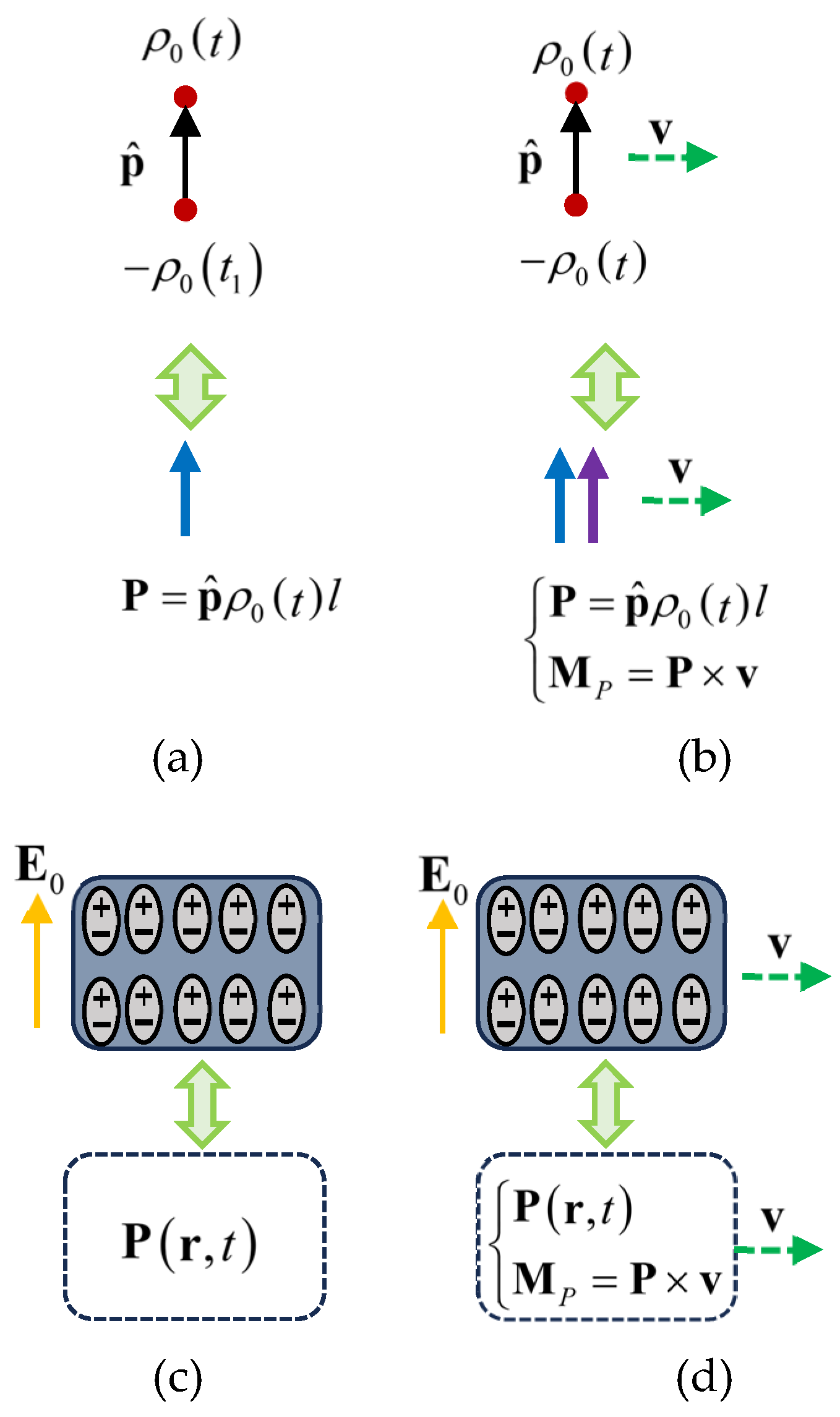
The analogy between modelling a moving dipole and modelling the polarization in a moving medium is sketched in Figure 2. For moving nonmagnetic media, we can amend the Chu formulation by directly taking the contribution of the motion-induced magnetization into account.
We extend the modification to magnetic media. We can check that a moving magnetic dipole with magnetization produces a polarization , which is observed in [21] for static magnetic dipole. Therefore, the amended Chu formulation Maxwell’s equations are
with , and . At a fixed point in a simple moving medium, we have the relationship of and .
To find the plane wave in a homogeneous moving medium with , we again assume that the wave propagates in parallel with the moving direction of the medium and the fields take the form of , . From the two curl equations in (34) we obtain
The determinant of the coefficient matrix must be zero in order that (35) has non-zero fields. Discarding the terms that contain with orders higher than one, we get the equation,
Solving equation (35) we get
From which we can get the phase velocity of the plane wave,
where ,. Obviously, (38) exactly agrees with the Fresnel’s coefficient (4).
In other formulations that the magnetization in the medium is described using the magnetization current with density of and zero electric magnetization charge, the inconsistency with the Fresnel’s coefficient also exists. Basically, they can be amended in the same way as we have proposed in amending the Chu formulation. It is straightforward to verify that the plane wave solutions of the corresponding amended formulations are compatible with the Fresnel’s coefficient.
5. Conclusions
We have clearly revealed that both the two inconsistencies in the conventional formulations of the Maxwell’s equations for moving media are caused by the fact that we have ignored the effect of the magnetization in moving electric dipoles and the polarization in moving magnetic dipoles in modelling the moving media. The two inconsistencies are closely related to each other and have existed in the classical electromagnetic theory for century long. The proposed modification of the Maxwell’s equations for moving media is simply a remedy for the two inconsistencies. With the amended formulations, we can correctly derive the Fresnel’s dragging coefficient from the Maxwell’s equations.
References
- Jackson, J.D. Classical Electrodynamics, 3rd ed.; Wiley: New York, 1998. [Google Scholar]
- Stratton, J.A. Electromagnetic Theory; McGraw-Hill Book Company Inc.: New York, 1941. [Google Scholar]
- Chaichian, M.; Merches, I.; Radu, D.; Tureanu, A. Electrodynamics. An Intensive Course; Springer-Verlag: Berlin Heidelberg, 2016. [Google Scholar]
- Penfield, P.; Haus, H.A. Electromagnetics of Moving Media; MIT Press: Cambridge, Massachusetts, 1967. [Google Scholar]
- Tai, T. A study of electrodynamics of moving media. Proc. IEEE 1964, 52, 685–689. [Google Scholar] [CrossRef]
- Cullwick, E.G. Electromagnetism and Relativity, 2nd ed.; Longmans Green & Co Ltd.: New York, 1957. [Google Scholar]
- Fano, R.M.; Chu, L.J.; Adler, R.B. Electromagnetic Fields, Energy, and Forces; John Wiley and Sons, Inc.: New York, 1960. [Google Scholar]
- Sommerfeld, A. Electrodynamics - Lectures on Theoretical Physics Vol. Ill; Academic Press, Inc.: New York, 1952. [Google Scholar]
- Fresnel, A. Lettre d’Augustin Fresnel a François Arago sur l’influence du movement terrestre dans quelques phenomenes d’optique. Annales de Chimie et de Physique 1818, 9, 57–76. [Google Scholar]
- Stachel, J. Fresnel’s (dragging) coefficient as a challenge to 19th century optics of moving bodies. In The Universe of General Relativity. Einstein Studies; Kox, A.J., Eisenstaedt, J., Eds.; Birkhäuser Boston, 2005; vol 11. [Google Scholar]
- Drezet, A. The physical origin of the Fresnel drag of light by a moving dielectric medium. Eur. Phys. J. B 2005, 45, 103–110. [Google Scholar] [CrossRef]
- Fizeau, M.H. On the hypotheses relating to the luminous æther, and an experiment which appears to demonstrate that the motion of bodies alters the velocity with which light propagates itself in their interior. Lond. Edinb. Dublin Philos. Mag. J. Sci. 1851, 2, 568–573. [Google Scholar] [CrossRef]
- Fizeau, M.H. XXXII. On the effect of the motion of a body upon the velocity with which it is traversed by light. Lond. Edinb. Dublin Philos. Mag. J. Sci. 1860, 19, 245–260. [Google Scholar] [CrossRef]
- Xiao, G.B. Re-interpreting the properties of the fields of a uniformly moving hertzian dipole in the vacuum. Next Res. 2025, 2, 100856. [Google Scholar] [CrossRef]
- Hnizdo, V. Magnetic dipole moment of a moving electric dipole. Am. J. Phys. 2012, 80, 645–647. [Google Scholar] [CrossRef]
- Field, J.H. Retarded electric and magnetic fields of a moving charge: Feynman’s derivation of Lienard–Wiechert potentials revisited. Preprint 2025, arXiv:0704.1574v3. [Google Scholar] [CrossRef]
- Xiao, G.B. Electromagnetic Sources and Electromagnetic Fields; Springer: Singapore, 2024; Chap. 3. [Google Scholar]
- Van Bladel, J. Relativity and engineering, 1st ed.; Springer: Berlin, Germany, 1984; pp. 70–72. [Google Scholar]
- Michielsen, B.L.; Herman, G.C.; de Hoop, A.T. Three-dimensional relativistic scattering of electromagnetic waves by an object in uniform translational motion. J. Math. Phys. 1981, 22, 2716–2722. [Google Scholar] [CrossRef]
- Deng, H.; Xiao, G.B.; Liu, G. An efficient method for calculating the Doppler spectrum of an arbitrarily shaped object in uniform motion. IEEE Trans. Antennas Propag. 2022, 70, 10894–10902. [Google Scholar] [CrossRef]
- Fisher, G.P. The electric dipole moment of a moving magnetic dipole. Am. J. Phys. 1971, 39, 1528–1533. [Google Scholar] [CrossRef]
Figure 1.
Trajectory of a moving Hertzian dipole for .
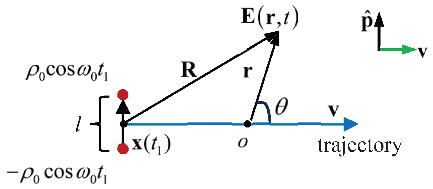
Figure 2.
Analogy between modeling the electric dipole and modelling the polarization in a medium. (a) Motionless electric dipole. (b) Moving electric dipole. (c) Motionless dielectric. (d) Moving dielectric.
Figure 2.
Analogy between modeling the electric dipole and modelling the polarization in a medium. (a) Motionless electric dipole. (b) Moving electric dipole. (c) Motionless dielectric. (d) Moving dielectric.
Disclaimer/Publisher’s Note: The statements, opinions and data contained in all publications are solely those of the individual author(s) and contributor(s) and not of MDPI and/or the editor(s). MDPI and/or the editor(s) disclaim responsibility for any injury to people or property resulting from any ideas, methods, instructions or products referred to in the content. |
© 2026 by the authors. Licensee MDPI, Basel, Switzerland. This article is an open access article distributed under the terms and conditions of the Creative Commons Attribution (CC BY) license (http://creativecommons.org/licenses/by/4.0/).
Copyright: This open access article is published under a Creative Commons CC BY 4.0 license, which permit the free download, distribution, and reuse, provided that the author and preprint are cited in any reuse.


