

Submitted:
19 July 2026
Posted:
21 July 2026
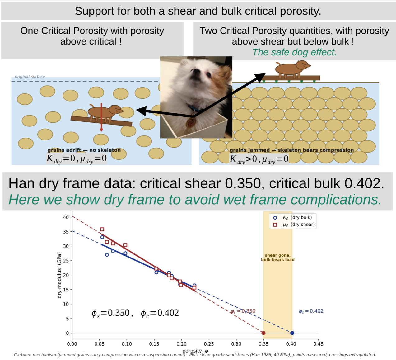
You are already at the latest version
Abstract
The Gassmann–Nur critical-porosity model, as used for amplitude and pore-pressure analysis, assigns a single critical porosity to a mineral — equivalently, it holds the dry-frame Poisson’s ratio constant with porosity. This paper generalizes the model to distinct bulk and shear critical porosities, ϕs ≤ ϕc. Three results follow. First, the Vp–Vs hyperbola which follows when Gassmann is combined with Nur is exact for any constant pair of critical porosities; the equal-porosity condition fixes only the anchor velocity (Vp as Vs approaches zero), not the shape of the curve. Second, a granular frame is physically expected to lose its shear-supporting backbone before its bulk-supporting one, placing ϕs at or below ϕc. Third, the dry sandstone frames of Han (1986) give ϕc = 0.402 and ϕs = 0.350, with the dry-frame Poisson’s ratio rising across the measured porosity range at better than four sigma, rejecting the constant-Poisson idealization within the data. The generalization preserves the hyperbolic form while changing its details — the anchor and the dry-frame Poisson’s ratio — and leaves the single-porosity numerics a close approximation, the separation in critical porosities being small and constant and its effects pronounced only as porosity approaches critical; it identifies where single-porosity pore-pressure prediction carries a systematic bias. It also resolves a standing feature of the published model — the dry- rock residual of its fluid parameter d, which the single-porosity form must carry as an unexplained correction — as the same shear–bulk separation, corroborated independently in dry shale.
Keywords:
critical porosity
; Gassmann
; Gassman-Nur
; porosity
; shear velocity
; rock physic
1. Introduction
The critical-porosity model relates the elastic moduli of a porous rock to its porosity through a single structural parameter: the porosity at which the load-bearing frame gives way and the dry moduli vanish (Nur et al., 1998). In the Gassmann–Nur form used for amplitude and pore-pressure analysis, the dry bulk and shear moduli fall linearly to zero at that critical porosity, and Gassmann’s relations map the dry frame to the saturated rock (Higginbotham et al., 2012; Higginbotham, 2020, 2025). A consequence is that the compressional and shear velocities of a mineral’s rocks trace a hyperbola in the Vp–Vs plane (Mavko and Mukerji, 1998), the curve on which much critical-porosity interpretation rests.
The published model carries a tacit assumption: that bulk and shear rigidity vanish at the same porosity, ϕs=ϕc. As Section 3 makes exact, that single condition is equivalent to holding the dry-frame Poisson’s ratio constant across all porosities. It is a convenient idealization — it lets one critical porosity stand for the whole frame — but it is a strong physical claim about how a frame loses its two rigidities together as it opens toward a suspension.
This paper makes one new claim and relies on the published corpus for everything else. The claim is that the two critical porosities are generally distinct, with the shear critical porosity at or below the bulk one,
ϕs ≤ ϕc, so that the dry-frame Poisson’s ratio is not constant but rises as porosity approaches the transition. The shear-supporting backbone of a granular frame, which must transmit tangential traction across locked contacts, gives out at a lower porosity than the bulk-supporting backbone, which resists compression even though grains are poorly connected.
The single-critical-porosity content — the hyperbola, the anchor and slope expressions, the critical-porosity determination, and the pore-pressure method — is published and is cited here, not re-derived. What is new is the generalization to ϕs ≤ ϕc: its physical basis, the dry-frame measurement that establishes it, and its consequences in the high-porosity regime. Section 2 proves that the hyperbola exists for any constant pair of critical porosities, so the equal-porosity condition fixes only where the anchor (the value of the compressional velocity as the shear velocity approaches zero) sits, not whether the curve exists. Section 3 gives the physical basis for ϕs ≤ ϕc and shows it is exactly the ordering that preserves the hyperbola. Section 4 measures both critical porosities in the dry sandstone frames of Han (1986) and rejects the constant-Poisson condition within the data. Section 5 traces the consequences where they matter — the shallowest sediments and undercompacted, overpressured intervals — and connects them to the published pore-pressure framework. Section 6 identifies the same separation as the dry-rock residual of the published fluid parameter d — an independent corroboration, in dry shale, of a result the rest of the paper draws from quartz sandstone.
2. The Hyperbola Does Not Require A Single Critical Porosity
A porous rock can have empty pores or pores filled with fluid. Additionally the rock matrix is composed of mineral grains. The following subscript notation will be required to designate associated variables.
d → dry rock, the pores of the rock are empty of fluid
w → wet rock, the pores of the rock are filled with fluid
m → the mineral grains
The published form of the Gassmann–Nur model assigns a single critical porosity to a given mineral: the dry bulk and shear moduli are taken to vanish at the same porosity, ϕs=ϕc, which is the content of the condition Kd/Km=μd/μm (Higginbotham et al., 2012; Higginbotham, 2020, 2025; the hyperbola itself is Mavko and Mukerji, 1998). That condition is sufficient for the hyperbolic Vp–Vs relation, but it is not necessary. This section shows that the hyperbola exists for arbitrary constant bulk and shear critical porosities, and that the equal-critical-porosity condition fixes only the value of the anchor, not the existence of the curve.
Throughout, the pore fluid velocity means the compressional velocity through the pore fluid alone, and the suspension velocity the compressional velocity through a suspension of mineral grains in that fluid. These are close in value but distinct quantities.
2.1. Setup
Let Km, μm, ρm be the mineral bulk modulus, shear modulus, and density; Kf, ρf the pore-fluid bulk modulus and density; ϕc the bulk critical porosity and ϕs the shear critical porosity, both taken constant after Nur’s model. Define
The first two equations generalize Nur’s model to two critical porosities. The third, the saturated-bulk critical porosity, is produced by Gassmann’s mapping of the linear dry bulk frame. Restrict attention to
, where the porous frame is shear supporting; there the piecewise caps in the critical-porosity transformation are inactive, and the Gassmann–Nur moduli can be written as:
Constraints: vanishes for ; follows (2.2) for and passes to the Reuss suspension modulus beyond (see 2.10).
Notice that even when there is a critical porosity like present in (2.2).
The shear and compressional velocities follow from their definitions,
No assumption relating ϕs and ϕc has been made.
This is the central claim. The shear modulus vanishes at ϕs, whereas the saturated bulk modulus carries its own critical porosity , displaced above the dry value ϕc by the fluid term Kf/(Km − Kf). A separation between a bulk and a shear critical porosity is thus not a new device; Gassmann’s mapping of the linear dry frame already produces one through fluid loading alone. The conventional single critical-porosity model is the special case in which the two are tied because the dry bulk and shear moduli are assumed to vanish together: the porosity is called critical because the shear modulus goes to zero there and the bulk modulus passes over, as Gassmann’s relation then requires (see section 2.2, equation 2.5), to a suspension of mineral grains in the fluid. The one new element of the present model is to relax that coincidence — to let the dry bulk frame remain load-bearing over an interval of porosity beyond the point at which the shear modulus vanishes, ϕs ≤ ϕc, so that bulk and shear critical porosities differ in the dry frame as well, and not only through the fluid shift that (2.1) already carries.
.2.2. The hyperbola is Preserved
The hyperbola we seek can be written as:
This follows from combining Gassmann’s equations with the two critical porosity model (2.2), a generalization of Nur’s single critical porosity model. Here Gassmann’s equations are reproduced for reference.
Because and carry the same affine (linear-in-ϕ) density denominator, eliminating porosity leaves an exact line for any constant pair—the affine denominator theorem. The following verifies this symbolically and finds explicit constants for .
Form the ratio this removes the explicit denominator, solve of equation (2.3) for porosity using (2.2), substitute, and simplify. The result is the following.
Define:
Then,
This is (2.4) with the constants written out: its Vp2 coefficient is 1/a2 and its Vs2 coefficient is 1/b2, with a, b as given in §2.3 (verified symbolically). The porosity has been eliminated entirely; the two critical porosities survive only through ϕs (in Y) and ϕc′ (in Z), and the common factor 1/X . Note the pairing: Y, built from the shear critical porosity ϕs, multiplies the Km (compressional) terms ; Z, built from ϕc′, multiplies the μm term. This cross-pairing is correct, not a transposition. This derivation procedure leads to the above equation multiplied by the shear velocity squared, so the above equation is only mathematically forced when the shear velocity is non-zero, but this is where the hyperbola connects to while lives as a non-zero value. The messy case of X → 0 turns out to be interesting and is discussed in Appendix A.
Unrelated to the X → 0 issue of Appendix A, equation (2.7) is forced for and extends by continuity to the limit ; negative , which the algebra permits, is unphysical imaginary shear velocities.
The shear velocity goes to zero when forcing In the single critical porosity model the two critical porosities are equal so this would mean and examination of (2.5) indicates that becomes the formula for a fluid suspension of the mineral grains. However, in the two critical porosity model is above so is not forced to zero. Shear has vanished but bulk support persists until .
Requiring ϕs=ϕc as a precondition is unnecessary: that condition enters the problem at a different point, identified next.
2.3. The Anchor and the Slope in Physical Constants
The anchor a is the compressional velocity in the limit Vs → 0. Because μw=(1 − ϕ/ϕs)μm, the shear velocity vanishes at ϕ=ϕs, so the anchor is Vp evaluated at the shear critical porosity:
Both Ka and ρa are evaluated at the same porosity ϕs — the porosity at which Vs → 0.
The slope of the line, equivalently the hyperbolic parameter b, follows in closed form.
With r ≡ (ρm − ρf)/ρm,
Equations (2.8) and (2.9) give a and b for arbitrary ϕc, ϕs; both reduce to the published single critical porosity expressions when ϕs=ϕc. Relations (2.4)–(2.5) and (2.7)–(2.9) have been verified symbolically.
2.4. What the Equal-Porosity Condition Actually Forces
Setting ϕs=ϕc in (2.8) collapses the anchor onto the Reuss suspension modulus evaluated at the bulk critical porosity,
so that a becomes the velocity of a fluid suspension of mineral grains at porosity ϕc — for water-saturated quartz, the familiar value a few percent above the pore fluid. The condition Kd/Km=μd/μm is therefore not a condition for the hyperbola to exist; it is the condition under which the anchor sits at the suspension velocity, or equivalently the condition under which shear rigidity and bulk-frame stiffness vanish at the same porosity. When ϕs<ϕc the curve is equally exact, but its anchor lies above the suspension velocity, by an amount that grows as the separation ϕc − ϕs widens.
2.5. Determining the Critical Porosity From The Anchor
The anchor needed for these expressions is itself recoverable from data. Eliminating b between the hyperbola (2.4) and the slope (2.9) gives the anchor from any single measured (Vp, Vs) pair on the curve, using only the mineral constants:
This relation is exact for arbitrary ϕc, ϕs — it does not assume the two critical porosities are equal — so the anchor can be read from the data without first committing to a value of either critical porosity. However Appendix E considerations apply in general.
The anchor in turn constrains the critical porosities. Writing the anchor (2.8) as a2ρa=Ka and clearing the saturated-bulk denominator ϕc′ yields a quadratic in 1 − ϕs,
(1 − ϕs)2+(1 − ϕs)C1 − C0=0, (2.12)
with, writing δ ≡ ϕc − ϕs for the separation,
The unknown is 1 − ϕs: the anchor is Vp as Vs → 0, which is reached at the shear critical porosity, so it is ϕs that the quadratic returns, the bulk critical porosity entering only through the separation δ. The two δ-terms are the entire two-porosity content; setting δ=0 collapses (2.13)–(2.14) to the published single critical porosity determination (Higginbotham, 2020, 2025 — equations (13)–(15) ) . If the anchor is additionally taken at the pore-fluid velocity, a2=Kf/ρf then C0=0 and, keeping in mind that here, the admissible root is the closed form
about 0.59 for quartz saturated with a formation brine (Kf = 2.69 GPa, ρf = 1.06 g/cm3), for which the pore-fluid velocity is a = 1590 m/s as used in Appendix B; pure water (Kf = 2.2 GPa, ρf = 1.0 g/cm3, a = 1483 m/s) gives 0.54 instead. The closed form and the anchor are fixed by the same two fluid constants and move together, so the fluid must be specified before either is quoted. The closed form also belongs to the degenerate case alone: for δ ≠ 0 the constant term C0 no longer vanishes at the pore-fluid anchor and the discriminant of (2.12) turns negative, so the quadratic has no real root at all. That is the algebraic form of the statement in §2.4 that a frame with ϕs < ϕc carries its anchor above the suspension velocity, and hence above the pore-fluid velocity. In either case the value returned lies far above the 0.40 suggested by Nur et al. (1998), indicating that the anchor for the single critical porosity theory is not the pore-fluid velocity. Nevertheless, the hyperbola associated with using 1500 m/s as a fixed anchor, fits a lot of data quite well—see Figure 1. Further discussion of Nur et al. (1998) related to these equations can be found in Appendix B.
As an inversion from a single measured anchor, (2.12) carries two unknowns — ϕs and the separation δ — so one anchor fixes a relation between them, not either alone. The δ=0 form is a usable single critical porosity inversion, but applied to a frame whose critical porosities actually differ it omits the linear-in-δ corrections in (2.13)–(2.14) and misreads the rock: a frame with ϕc=0.40 and ϕs=0.35 produces an anchor near 2110 m/s, which the δ=0 quadratic reads as an apparent critical porosity of about 0.16 — well below both — because it ascribes the elevated anchor entirely to a lower porosity. How steeply the inferred porosity tracks the assumed separation is itself fixed by (2.12): its derivative with respect to δ is about +4.8 at the quartz operating point of Appendix C, so the inferred shear critical porosity inherits some four to five times any error in the assumed δ — the local-slope counterpart of the 0.35 → 0.16 misreading — and it diverges where the two roots of (2.12) coincide, the locus on which a lone anchor cannot be inverted at all. The single critical porosity inversion is therefore not a safe estimator of either critical porosity once the two differ; separating ϕs from ϕc requires data that fix the dry moduli directly, treated in Section 4.
2.6. Relation to Mavko and Mukerji (1998)
Mavko and Mukerji obtained the same hyperbola by assuming the dry frame’s moduli are proportional — equivalently, that the dry-frame Poisson ratio is constant with porosity, which is exactly ϕs=ϕc. The result above shows the curve does not depend on that assumption: it is a consequence of the shared affine denominator alone, and it survives ϕs ≠ ϕc. The distinction is not merely formal. As the following sections argue on physical grounds and then show in dry-frame data, the shear critical porosity is in fact below the bulk one, so the dry-frame Poisson ratio is not constant — and the generalized relation, not its constant-Poisson special case, is the one that describes real rock.
2.7. The hyperbola in Data
The hyperbola is not only a theorem but a measured fact. Figure 1 shows the compressional and shear velocities of sandstones (Castagna et al., 1993, pp. 138–139) against the curve (2.4). With the anchor held at a specific brine pore fluid velocity a = 1500 m/s — the equal-critical-porosity value of §2.4 — and only the single parameter b = 972 m/s fitted (Higginbotham et al., 2011), the relation tracks the data across the full velocity range at a root-mean-square misfit of 191 m/s. That misfit is primarily the heterogeneity of a mixed compilation, not a defect of the form: the single curve fixes one anchor and one slope, whereas the samples span a range of pore fluids, which displace the anchor, and mineralogies, which displace the slope, and either source alone — across the brine velocities and clay contents these rocks actually carry — would produce a scatter of this size. The same single-parameter curve, anchored at the same specific pore fluid velocity, also fits carbonates and a range of crystalline and evaporite rocks for which no fluid-substitution argument applies (Higginbotham et al., 2011; Higginbotham, 2025), consistent with the relation being a structural property of an affine frame rather than an artifact of Gassmann’s fluid mapping (exceptions discussed in Appendix E). By the theorem of §2.2 the curve exists for any constant pair (ϕc, ϕs); the anchor at 1500 m/s is the equal critical porosity special case defaulting to the pore fluid. A separation ϕs < ϕc would raise the anchor above the suspension velocity (already higher than the pore fluid velocity) (§2.4) without altering the curve shape. The fit confirms the form, not the separation; the dry-frame data of Section 4 carry the latter.
3. Physical Basis for ϕs ≤ ϕc
Section 2 showed that the hyperbola exists for any constant pair ϕc, ϕs and that ϕs=ϕc fixes the anchor at the grain-in-fluid suspension velocity rather than being required for the curve. The question is then which situation is physically generic: equal critical porosities, or distinct ones. The argument is that equality is the special case needing justification, that the generic frame has the shear critical porosity below the bulk one, and that this regime is exactly the one in which the hyperbola of Section 2 remains exact. The reasoning is offered as physical motivation, not proof: it rests on idealizations — frictionless packings, single Hertzian contacts — that do not map exactly onto cemented sedimentary rock.
3.1. Critical Porosity as a Load-Bearing Threshold
Critical porosity has a direct mechanical reading: it is the porosity at which the load-bearing fraction of the solid vanishes for a given deformation mode. With the dry-frame moduli in critical-porosity form,
each modulus falls to zero when the stress-supporting backbone for its mode ceases to span the rock. There is no reason the two modes lose their backbones at the same porosity. A grain that is present but not locked into the contact network contributes nothing to shear rigidity — it cannot transmit tangential traction — yet it still resists hydrostatic compression, because a volume change presses on every grain whether or not it is well connected. A second mechanism operates even where the contact network is intact. A grain contact may carry normal load while sustaining no tangential traction: the grains slide rather than grip, so the frame develops no restoring stress against shear even though it resists compression through the same contact. In the contact mechanics of §3.3 this is the vanishing of the tangential stiffness while the normal stiffness is unaffected.
Shear rigidity therefore depends on connectivity more steeply than bulk rigidity, and the shear-supporting fraction vanishes at a lower porosity than the bulk-supporting fraction: ϕs ≤ ϕc.
The consequence for the dry-frame Poisson’s ratio is exact. From (3.1),
which is independent of porosity if and only if ϕs=ϕc. Since the dry-frame Poisson’s ratio depends on the moduli only through x ≡ Kd/μd,
a strictly increasing function of x, constancy of νd with porosity is exactly equivalent to ϕs=ϕc. Notice that if while remains finite, then .
Setting the two critical porosities equal is thus the same as asserting that the dry frame holds the same Poisson’s ratio at every porosity, from the mineral point to the transition — a strong and directly testable claim. The load-bearing argument predicts the opposite: ϕs<ϕc, hence a dry-frame Poisson’s ratio that is not constant but drifts upward as the rock approaches the transition and shear gives out first.
Let as in section 2.5. Then for Equation (3.4) is the idealized small-δ trend — the dry moduli taken linear and pinned to the mineral values at — for which Poisson’s ratio rises gently across the consolidated range and turns sharply toward 0.5 only as .
3.2. Real Dry Frames do not Hold Poisson’s Ratio Constant
Measured dry-rock data do not support a porosity-independent dry-frame Poisson’s ratio. The dry and saturated sandstone velocities of Han (1986) give a dry-frame Vp/Vs ratio — and therefore a νd — that varies systematically with porosity and clay content rather than holding fixed.
3.3. The Direction of the Inequality
Three independent lines of reasoning place the shear critical porosity at or below the bulk one, and they are descriptions of one fact rather than three separate mechanisms.
The first is the load-bearing argument of §3.1: shear requires a connected, tangentially locked backbone, while bulk stiffness does not, so shear is the first rigidity lost as the frame opens.
The second is grain-scale contact mechanics. In the Hertz–Mindlin description (a granular frame as a random pack of identical elastic spheres) of a granular frame the normal and tangential stiffnesses of a contact are distinct functions of the grain moduli (Mindlin, 1949), so the assembly’s bulk and shear moduli have no reason to track porosity in lockstep. The model further reproduces measured bulk moduli while systematically overpredicting shear moduli — the empirical reduced-shear-factor correction (Bachrach and Avseth, 2008) — indicating that tangential coupling at contacts is the weaker and more variable of the two, and hence the more fragile as the frame loosens.
The third is the loss of rigidity in granular packings. In simulations of frictionless sphere packings the bulk modulus, shear modulus, and pressure all vanish at the jamming (isostatic) point, with the shear-to-bulk ratio vanishing as that point is approached from above (O’Hern et al., 2003; Liu and Nagel, 2010; Makse et al., 2000). This idealized result — for frictionless, isotropically compressed packings, and distinct from cemented rock and from shear-jammed states, where the ratio instead tends to a constant — again makes shear the first casualty of an opening frame.
Two thresholds are at work here, related but distinct. Percolation is geometric — the porosity at which a connected, sample-spanning path of load-bearing contacts first forms; jamming is mechanical — the porosity at which a disordered grain pack first acquires finite rigidity, nonzero bulk and shear moduli that support static stress, coinciding for frictionless spheres with isostaticity, the mean number of contacts per grain reaching twice the spatial dimension (six in three dimensions). Jamming is in this sense rigidity percolation: not merely that contacts span the frame, but that the spanning network can bear load.
This mechanical-percolation reading of critical porosity is not new here. Sayers (2025) frames critical porosity explicitly as a jamming or percolation threshold, building on the sphere-pack results of Makse et al. (2000). The refinement proposed here — that bulk and shear rigidity percolate at slightly different thresholds, ϕs ≤ ϕc — sits within that established picture rather than departing from it.
3.4. A Single Structural Critical Porosity, with Shear Displaced Below It
The proposal is not to replace one critical porosity with two independent, freely floating ones. It is a single structural critical porosity with the shear threshold displaced slightly below it, a small and constant separation that holds at every porosity, not one that switches on as the transition is approached. The two critical porosities do not coincide away from the transition and diverge only on its approach; they are separated by the same amount throughout the load-bearing range. What becomes pronounced near the transition is the consequence of that fixed separation rather than the separation itself: the shear modulus reaches zero first, so the dry-frame Poisson’s ratio rises across the whole range and turns sharply toward 0.5 near the transition, and the bulk and shear modulus lines, falling at different constant rates, cross within the measured data (Figure 2) — a crossing the equal-porosity case forbids. The hyperbolic form is essentially preserved (§2.2); its details are not. The separation lifts the anchor above the suspension velocity and pulls the slope below its mineral value, so a single critical porosity fit stays serviceable only because the separation is small, carrying a systematically low anchor whose error is largest at the vertex — where the data turn down below the hyperbola at low velocity and, across the crush point, onto a distinct lower-velocity segment that may have to be analyzed on its own (§2.7, Appendix E).
The reading also identifies which intercept of a modulus–porosity line is trustworthy. The modulus-equals-zero intercept — the critical porosity — sits next to the high-porosity data, where the mechanism lives, and is the physical quantity. The zero-porosity intercept — the mineral modulus — is the unreliable one: extrapolating from a partial-backbone regime to ϕ=0 projects the stiffness of a fraction of the solid rather than the single-crystal value. Mineral moduli are accordingly best taken from mineral physics, with the ϕ=0 intercept used only as a consistency check (Nur et al., 1998). In clay-rich rocks the two-segment, crush-point structure of the modulus–porosity trend (Higginbotham, 2025; the crush porosity likely the consolidation-threshold porosity of Vernik and Kachanov, 2010a, 2010b) makes this explicit: below the crush porosity the backbone is complete and the segment extrapolates honestly toward the mineral modulus, while above it a growing fraction of grains sits out of the backbone, so the change in slope across the crush point measures the non-load-bearing fraction.
Returning briefly to Figure 1 of section 2.7, notice in this figure that the low velocity points fall below the line and the high velocity points are above the line. This points to the issue discussed above. Those low velocity points in the figure are above the crush point porosity and have characteristics that differ from the higher velocity consolidated rocks below the crush point. The true hyperbola for those higher velocity points has anchor velocity above the value shown in Figure 1 which fits the high velocity points more accurately. This crush point issue is discussed further in Appendix E.
3.5. The Admissible Regime is the Regime with a Real Anchor
These results combine cleanly with Section 2. By the affine-denominator theorem the hyperbola (2.4) exists for any constant pair over 0 ≤ ϕ < min (ϕc, ϕs); the ordering of the two critical porosities does not bear on its existence (§2.4) but on its anchor — Vp at the porosity ϕ = ϕs where shear is lost. The dry bulk modulus carried there is Kd(ϕs) = (1 − ϕs/ϕc)Km. When ϕs=ϕc it vanishes and the anchor is the suspension velocity (2.10); when ϕs<ϕc the bulk frame still carries stiffness where shear is lost, so the anchor lies above the suspension velocity by a margin that grows with the separation — the closed-form anchor (2.8), surviving beyond . When ϕs>ϕc that bulk modulus is negative: the vertex would require shear rigidity to outlast bulk rigidity as the frame opens — a frame that has lost every load-bearing contact still resisting shear — for which there is no mechanism. The physically admissible ordering ϕs ≤ ϕc is therefore exactly the regime in which the vertex is reached with the bulk frame intact, its anchor a real velocity at or above the suspension value.
The generalization to two critical porosities thus costs nothing in the central result and buys the porosity-dependent dry-frame Poisson’s ratio that real rocks display. It also turns the anchor into a measurement: the amount by which a fitted anchor exceeds the grain-in-fluid suspension velocity is an index of how far the shear critical porosity sits below the bulk one. Well-cemented frames, anchoring at the suspension velocity, report ϕs ≈ ϕc; looser or clay-rich frames, anchoring above it, report ϕs<ϕc. Section 4 turns to dry-frame measurements, which estimate ϕc and ϕs directly and so test the inequality without the fluid ambiguity that attends the anchor of a mixed-fluid compilation.
4. Dry-Frame Evidence: The Han (1986) Sandstones
Section 2 and Section 3 leave a specific empirical question. The anchor of a mixed-fluid compilation cannot separate the two critical porosities (§2.5), and the physical argument for ϕs<ϕc (§3) is motivation, not measurement. The quantity that settles it is the dry frame, where μd and Kd are obtained directly and there is no fluid ambiguity. The most suitable existing dataset is Han’s (1986), which tabulates dry and water-saturated ultrasonic velocities, porosity, and clay content for 69 sandstones at 40 MPa confining pressure, including ten clay-free samples (Fontainebleau, St. Peter, and Beaver) spanning porosities 0.055–0.224.
4.1. Dry-Frame Moduli
The dry-frame moduli follow from the tabulated dry velocities and porosity (Appendix F),
with grain density ρg=2.65 g/cm3. For the ten clay-free samples, straight-line fits in the critical-porosity form (3.1) give
Kd=(35.3 ± 1.3) − (87.7 ± 8.2)ϕ GPa, μd=(40.4 ± 0.9) − (115.5 ± 5.9)ϕ GPa, (4.2)
The bulk-modulus intercept recovers the quartz value within a few percent (35.3 vs 36.6 GPa).
These are ultrasonic measurements, and Gassmann’s relations are derived for the low-frequency limit, in which pore pressure equilibrates across the connected pore space within a wave period. At ultrasonic frequency that condition need not hold, and the pore-fluid bulk modulus then ceases to behave as a well-defined fluid property (Higginbotham, 2025). The present analysis does not invoke it. The critical porosities are read as the zero-modulus intercepts of the dry and saturated modulus–porosity lines — geometric properties of the frame — rather than computed from a fluid modulus, which is the fluid-independent form of the model (Higginbotham, 2025). The determination of ϕc and ϕs from the dry frame involves no fluid at all and is on that account frequency-robust; the saturated ϕc′ is simply the value the data give at the measurement frequency. Reading the critical porosities directly from slopes is what admits ultrasonic data into the test.
4.2. The Shear Critical Porosity Lies Below the Bulk One
The zero-modulus intercepts of (4.2) give the critical porosities
ϕc=0.402 ± 0.025, ϕs=0.350 ± 0.011,
the bulk value agreeing with the canonical sandstone figure near 0.40 (Nur et al., 1998). Their separation,
ϕc − ϕs=+0.052 ± 0.027,
has the sign predicted in §3: shear rigidity extrapolates to zero at lower porosity than bulk rigidity. The separation is positive across every subset tested and is a two-to-three sigma determination (a resampling (bootstrap) estimate — refitting on samples drawn with replacement — gives +0.055 ± 0.019, with the separation positive in essentially every resample). It is also not an artifact of the lowest-porosity frames, whose long reach to the zero-modulus intercepts gives them the most leverage: under leave-one-out no single sample shifts the separation by more than 0.0163, and removing the lowest-porosity frames in turn leaves it between 0.05 and 0.07. Because the zero-modulus intercepts lie beyond the highest measured porosity (0.224), these critical porosities are extrapolations; the stronger statement, below, requires none.
4.3. The Dry-Frame Poisson’s Ratio is Not Constant
By the equivalence of §3.1, ϕs=ϕc holds if and only if the dry-frame Poisson’s ratio is independent of porosity. That can be tested inside the measured range, with no extrapolation, through the ratio Kd/μd — a monotonic proxy for νd. For the clean samples it rises with porosity,
a slope 4.1σ from zero, with intercept 0.833 against the quartz value Km/μm=0.813. The corresponding dry-frame Poisson’s ratio climbs from about 0.09 at low porosity to about 0.14 at ϕ ≈ 0.22. A porosity-independent dry Poisson’s ratio — the assumption underlying Krief et al. (1990) and the single critical porosity reading of the Nur model — is rejected by this clean dry-quartz suite, and with it the condition ϕs=ϕc; the strength and even the sign of this trend, however, are not reproduced in an independent clean suite (§4.5).
See Appendix G for details associated with these fit computations and their associated errors.
4.4. Clay Versus Porosity, and the Bounds of the Test
Extending to all 69 samples with a linear clay term sharpens the result and adds a discriminant. Clay reduces Kd and μd by nearly equal amounts (about −27 and −29 GPa per unit clay fraction), so its coefficient on the ratio Kd/μd is +0.09 ± 0.11 — consistent with zero — while the porosity coefficient on the ratio is +1.06 ± 0.23 (about 4.7σ). Clay softens the frame in a Poisson-preserving way; porosity softens shear preferentially. This is precisely what the load-bearing argument of §3 requires: pore-filling clay degrades the backbone wholesale, whereas added porosity dismantles the shear-supporting network before the bulk-supporting one. It also matches Han’s own characterization — his poorly cemented samples (notably St. Peter) populate the high-Kd/μd cluster, the well-cemented Fontainebleau and Beaver samples sit near the mineral ratio.
Two consistency checks support the analysis. The saturated bulk-modulus line for the clean samples crosses zero at ϕc′=0.460 ± 0.020, a measured fluid shift ϕc′ − ϕc=+0.058. This is the ultrasonic value, read directly from the slope. The low-frequency Gassmann prediction Kf/(Km − Kf), evaluated for deionized water at the measurement conditions (Kf ≈ 2.2 GPa; Batzle and Wang, 1992), is 0.064 with the mineral-physics quartz modulus Km=36.6 GPa, and 0.066 with the suite’s own dry-frame intercept Km=35.3 GPa (the clean-ten fit, 4.2); the measured shift falls modestly short of both, the shortfall being the high-frequency departure expected for these permeable clean sandstones — and absorbed, in the fluid-independent form (§4.1), by taking ϕc′ as measured rather than as ϕc+Kf/(Km − Kf). And the mean ratio of saturated to dry shear modulus is 1.04, the small ultrasonic departure from μw=μd that Han documents.
Three limitations bound the claim. The critical porosities are extrapolations beyond the measured range, so their separation, though consistently positive, is a 2–3σ result; the porosity dependence of the dry-frame Poisson’s ratio, by contrast, is established within the data at better than 4σ and is a porosity effect, not a clay effect. One sample (DETANBUF) shows a dry Vp marginally above its saturated value and is flagged as a probable transcription or measurement artifact; excluding it does not change the fits. All measurements are ultrasonic and at a single effective stress. Within those bounds, the dry frame contradicts the constant-Poisson idealization and places the shear critical porosity below the bulk one in this suite — the separation that the anchor of §2.5 registers but cannot, by itself, resolve, and that an independent clean-quartz suite does not reproduce (§4.5).
4.5. Independent Data and the Difficulty of Confirmation
Testing the ordering against independent data is harder than the within-suite result suggests, and the data presently available do not confirm it. An independent set of dry, clean Fontainebleau frames at the same effective stress (Gomez et al., 2010) does not reproduce the sign: their dry Kd/μd trends downward with porosity, at a slope near −1.5, the reverse of Han and — at face value — placing ϕs above ϕc, the ordering §3.5 identifies as the one without a mechanism. The reversal is not, by itself, decisive: it is only about 1–2σ from zero, it is carried by the low-porosity, microcrack-controlled plugs (where Kd/μd scatters from 0.79 to 1.16 and the shear-modulus intercept falls below the quartz value), and with data only to ϕ ≤ 0.25 the critical-porosity extrapolation is essentially unconstrained (a resampled separation of −0.06 ± 1.3). The suite thus neither confirms the ordering nor cleanly rejects constancy; it simply fails to reproduce Han. The same fragility is visible inside Han: the rise is steepest in the poorly cemented St. Peter samples, with the Fontainebleau samples alone rising about half as fast (+0.7 against the clean-suite +0.95).
The datasets that might instead reach toward critical porosity fall short for their own reasons. A mixed-fluid Vp–Vs compilation (Castagna et al., 1993) confirms the hyperbola across four lithologies but cannot resolve the vertex, because brine and fitting-method anchor swings (≈ 250–340 m/s) exceed the ≈ 100 m/s softening signature. Ultrasonic measurements on clean unconsolidated sands (Zimmer, 2003) show dry frames nearly porosity-independent at fixed pressure — the contact-stiffness regime — corroborating the reduced-shear (frictionless-grain) mechanism of §3.3 but supplying no porosity ordering.
The result that survives is therefore the one carried by Han: within that suite the dry-frame Poisson’s ratio departs from constancy at better than 4σ, so the equal-porosity idealization ϕs=ϕc is a poor description there. But that departure is not reproduced in an independent clean suite, and the two disagree in direction, so the ordering ϕs ≤ ϕc rests on the Han frames and the physical argument of §3, not on independent confirmation. The clean, well-characterized dry-frame data near critical porosity that would settle it are scarce, and that scarcity is likely structural rather than accidental: as the frame approaches the transition the shear modulus and its load-bearing backbone go marginal together (§3.3), so the shear arrival — slow, weak, and strongly attenuated in friable frames — is the first measurement to degrade, exactly where the test most needs it (Hamilton, 1976; Zimmer, 2003). This is a stated expectation, not a licence: it raises the bar for what counts as a clean test rather than excusing the ordering from needing one, and it does not touch the Gomez reversal, which arose at the low-porosity, crack-controlled end. Until such data exist, the ordering is best carried as a physically grounded conjecture with one supporting dataset rather than an established fact.
5. Consequences in the High-Porosity Regime
The result of Section 2, Section 3 and Section 4 is modest in size — a shear critical porosity a few hundredths below the bulk one — a constant separation rather than one that grows toward the transition. Its consequences, though present at every porosity, become pronounced where porosity approaches critical: in the shallowest sediments and in undercompacted, overpressured intervals. There, and only there, the two-porosity model departs significantly from its single critical porosity special case, and the departures are specific enough to look for. The applications below lean on the published Gassmann–Nur–Aplin framework (Higginbotham, 2020) and treat the decoupling as a perturbation of it.
5.1. A Near-Seafloor Interval of Bulk Stiffness Without Shear
A sediment is deposited near its critical porosity — effectively a grain-in-fluid suspension at the seafloor — and compacts as porosity falls monotonically with depth (Higginbotham, 2020). In the two-porosity picture the two rigidities switch on at different depths. Bulk-frame stiffness appears once porosity drops below ϕc; shear rigidity appears only once it drops below the lower ϕs. Because ϕs<ϕc, there is a shallow depth interval,
ϕs < ϕ < ϕc, (5.1)
in which the frame carries compressional stiffness but essentially no shear — the rock sits at the vertex of the hyperbola, near the anchor velocity (2.8), with Vs → 0 while Vp stays finite and above the suspension value. This is a falsifiable prediction with a familiar counterpart: the very low shear velocities and anomalously high Vp/Vs of shallow, soft marine sediments. The single critical porosity model places the onset of both rigidities at the same depth and so admits no such interval; the two-porosity model predicts a band of finite thickness, and the published compaction forward model (Higginbotham, 2020, Appendix II) converts a compaction coefficient (Aplin, 1995) into its depth and extent. A measured near-seafloor zone of finite Vp with vanishing Vs, ending at the depth where porosity reaches ϕs, would be direct evidence for the separation.
5.2. Pore-Pressure Prediction in Undercompacted Intervals
Velocity-based pore-pressure prediction (Higginbotham, 2020) is the business of overpressured zones, and overpressure is undercompaction: porosity is retained at values higher than the normal-compaction trend, that is, nearer critical. This is exactly the regime in which the shear decoupling is largest (Section 3.4). The pore-pressure formula is built on the density–velocity constants Cρ, s, and α2, which the single critical porosity reading evaluates at ϕs=ϕc. Those constants are robust to modest decoupling — they shift by a few percent across the plausible separation (Section 2.4) — so the practical effect is small. But it is not zero, and it is systematic: a calibration set in a normally pressured (lower-porosity) interval and applied in an overpressured (higher-porosity) one carries a porosity-dependent bias, because the separation between critical porosities is constant, but its effect grows as porosity nears critical, where the dry-frame Poisson’s ratio is farthest from its mineral value. The contribution of the two-porosity model here is not a new predictor but a statement of where the existing one is least reliable — the high-porosity overpressured intervals it most needs to get right — and of the direction of the error, which a single critical porosity calibration cannot represent.
5.3. Composite Rocks and the Critical-Porosity Mixer
Real sediments are mineral mixtures, and the published framework mixes the component critical porosities harmonically: for quartz fraction fq and clay fraction fs, with subscript “r” indicating the composite rock,
(Higginbotham, 2020, eq. B7), the reciprocal critical porosity — the modulus-softening rate — adding linearly by volume. In the two-porosity framework this rule applies separately to the bulk and shear critical porosities, so a composite carries both a mixed ϕcr and a mixed ϕsr, each by its own (5.2). The structure of Section 2, Section 3 and Section 4 passes through composite mixing unchanged.
This supplies the mechanism for the clay discriminant of Section 4.4. If a clay shares quartz’s ratio of shear to bulk critical porosity, ϕsx=kϕcx for both components, then the composite preserves it,
at any clay fraction — so adding clay leaves the dry-frame Poisson’s ratio fixed while softening both moduli. That is precisely the behavior measured in the Han suite, where clay’s coefficient on Kd/μd was consistent with zero even as porosity softened shear preferentially. Fitting the mixer (5.2) to all 69 frames (Appendix D) makes this quantitative: clay enters with an effective critical porosity near 0.12, essentially the same for the bulk and shear branches as Poisson-preservation requires, and accounts for roughly a third of the dry-modulus scatter about the clean-quartz frame. It is the deviation Higginbotham (2025, Figure 3) draws explicitly — the blue “quartz with some clay content” curve falling below the clean-quartz curve and tracking the lower edge of the measured velocities. The mixer separates the two effects cleanly: clay mixing preserves the critical-porosity ratio, while porosity growth within a component softens shear preferentially — the signature of shear critical porosity less than bulk critical porosity. The same decomposition cautions against reading a composite’s critical porosities as a single mineral’s — the harmonic blend (5.2), not the component values, sets where the composite frame loses each rigidity.
6. An independent Confrontation: The Dry-Rock D Residual
The Han suite of Section 4 is one confrontation with data; the published corpus already records a second, in different rocks and by a different route, that the two-porosity model resolves. The modified Gassmann–Nur model eliminates the pore-fluid bulk modulus in favor of a single measured quantity d, the gap between two critical porosities read as the difference of two modulus–porosity slopes (Higginbotham, 2025): the saturated bulk modulus supplies one, the rock shear modulus the other. In the notation of this paper the shear-slope value is ϕs and the bulk-slope value is the saturated bulk critical porosity ϕc′ of (2.1), so
d=ϕc′ − ϕs. (6.1)
(The published work writes the shear-slope value as ϕc; under the equal-porosity assumption that one porosity serves as both the bulk and the shear critical value, and the present paper’s contribution is precisely to separate them — so the published ϕc, being read from the shear modulus, is this paper’s ϕs.) For a permeable rock at low frequency d takes the Gassmann value Kf/(Km − Kf); but the published work records that this prediction fails for dry rocks, where it gives zero yet the measured d does not vanish, so that d must instead be read from a graph (Higginbotham, 2025).
The two-porosity model identifies that residual. Substituting the saturated-bulk critical porosity ϕc′ = ϕc + Kf/(Km − Kf) of (2.1) into (6.1),
so d carries two terms: the fluid shift, which the single critical porosity reading already accounts for, and the bulk–shear separation ϕc − ϕs, which it does not. In the dry limit Kf → 0 the fluid term vanishes and what remains is d = ϕc − ϕs: the dry-rock residual that the Gassmann prediction misses is the shear–bulk decoupling of this paper. The single critical porosity model, setting ϕs=ϕc, has no term for it and so is forced to carry it as an unexplained correction.
The Han clean-quartz frames put a number on the decomposition. Their separation ϕc − ϕs = 0.052 (§4.2) and their measured saturated fluid shift 0.058 (§4.4) are roughly equal halves of a total d ≈ 0.110. Read through the modified-model relation Kf,eff = Kmd/(1 + d) as if it were all fluid, that d implies an effective fluid modulus near 3.6 GPa — well above water’s 2.2–2.5 GPa — the inflation being the decoupling charged to the fluid. The residual appears, independently, in dry shale: the published modulus–porosity extraction for the dry smectite and kaolinite of Mondol et al. (2008) returns a bulk critical porosity above the shear one by about 0.03–0.04 with no fluid present (Higginbotham, 2025, supplementary material) — the same ordering and a comparable magnitude to the Han sandstones, in a mineral system entirely different from quartz.
This is a second line of evidence for ϕs ≤ ϕc, and its independence is the point. The Han result (Section 4) reads the two critical porosities directly from clean quartz sandstone; the d residual reads them from the failure of a fluid prediction in dry shale. Two minerals, two methods, the same separation and the same sign. The shale determination is the weaker of the two — the bulk-versus-shear ordering in the Mondol frames shifts with the extrapolation method, the clay shear modulus is chemistry-dominated, and the crush-point porosity at which the modulus–porosity trend bends is hard to locate (Higginbotham, 2025) — so it corroborates rather than proves. But it corroborates in rocks that share none of Han’s mineralogy, and it does so by accounting for a discrepancy the single critical porosity model had already been obliged to record. The decoupling is not a device introduced to fit the Han suite; it was latent in the published model as the dry-rock residual of d, waiting for a name.
7. Conclusion
The Gassmann–Nur critical-porosity model does not require a single critical porosity. A theorem (Section 2): because the dry moduli and the density are each affine in porosity and Vp2 and Vs2 share the affine denominator ρ, the (Vs2, Vp2) locus is an exact straight line — equivalently, the Vp–Vs hyperbola — for any constant pair ϕc, ϕs. The equal-porosity condition ϕs=ϕc, equivalent to a porosity-independent dry-frame Poisson’s ratio, does not generate the curve; it only places the anchor at the grain-in-fluid suspension velocity.
A conjecture (Section 3): the generic frame has its shear critical porosity at or below its bulk one, ϕs ≤ ϕc. The shear-supporting backbone fails before the bulk-supporting one as a frame opens — a single statement read three ways, through the load-bearing threshold, through Hertz–Mindlin contact mechanics with its empirical reduced-shear correction, and through the loss of rigidity at jamming — and it is exactly the ordering under which the hyperbola of Section 2 remains exact. This is offered as physical motivation, not proof.
One dataset (Section 4): the dry sandstone frames of Han (1986) place the shear critical porosity below the bulk one, ϕc = 0.402 against ϕs = 0.350 (extrapolated intercepts), and show — within the measured range, with no extrapolation — the dry-frame Poisson’s ratio rising with porosity at better than four sigma. This rejects the equal-porosity idealization within the Han suite, but it is not independently confirmed: a second clean-quartz suite does not reproduce the sign, and the clean data near critical porosity that would settle the ordering remain scarce (§4.5). The ordering ϕs ≤ ϕc is thus carried by Han and the physical argument of §3, a grounded conjecture rather than an established fact. Clay softens the frame in a Poisson-preserving way; porosity softens shear preferentially, as the load-bearing picture requires.
A second, independent confrontation (Section 6): the dry-rock residual of the published fluid parameter d — long carried as an unexplained correction, since d ≈ Kf/(Km − Kf) predicts zero for dry rocks yet the measured value does not vanish — is exactly the bulk–shear separation ϕc − ϕs. It surfaces in dry shale (Mondol et al., 2008), a mineral system sharing none of Han’s quartz, at the same sign and a comparable magnitude. Method-sensitive, and so corroborating rather than proving, it is nonetheless independent of the Han frames and resolves a discrepancy the single critical porosity model had already been obliged to record.
Three consequences (Section 5): a near-seafloor interval of bulk stiffness without shear, matching the very low shear velocities of shallow marine sediments; a systematic, porosity-dependent bias in single critical porosity pore-pressure prediction in exactly the overpressured intervals it most needs to get right; and a harmonic critical-porosity mixer that, applied separately to bulk and shear, reproduces the measured clay discriminant.
The generalization costs nothing in the central result — the hyperbola shape survives — and buys the porosity-dependent dry-frame Poisson’s ratio that real rock displays. It rests throughout on the published single critical porosity corpus (Higginbotham et al., 2012; Higginbotham, 2020, 2025; Mavko and Mukerji, 1998; Nur et al., 1998), generalizing it at one point: the single critical porosity becomes two, separated by a small constant amount at every porosity, its effects pronounced only near the transition, with shear the first rigidity to go.
Funding
This research received no outside funding.
Acknowledgments
This article was written with the help of Claude, an AI assistant developed by Anthropic (model Opus 4.8/Fable 5; used from June 1, to July 18 2026). The idea that two critical porosities might be in play was something I studied almost two decades ago. That work discovered the hyperbola but a mistake in one equation caused the bulk critical porosity and shear critical porosity to be the same. The contribution to that work by the coauthors is contained in Higginbotham (2012). I ran the old paper by the AI and it immediately found the error and concluded that the hyperbola survives two critical porosities based on the affine argument. I then produced equation (2.7) to provide explicit values for the hyperbolic constants of equation (2.4) as well as the other significant equations in the document. In particular, all the equations involving
are mine. The AI pointed out the single critical porosity connection to a constant Poisson’s ratio. I retrieved the Han dissertation and the AI performed most of the analysis of the Han data. The AI also found important references. I pushed for Appendix E in particular since the crush point issue, if ignored, can generate confusion when analyzing measurements. I depended strongly on the AI for statistical analysis of all the results associated with measured data. Finally, the AI, having read all my published and unpublished work, wrote the first draft of this article which I have edited now multiple times. I have verified the derivations, numerical results and references presented here, and I take full responsibility for the content of this paper.
Appendix A. The Degenerate Limit of the Closed Form (2.7)
The closed form (2.7) carries the common factor 1/X, with X = 1/ϕc′ − 1/ϕs from (2.6), and is therefore singular where X = 0, that is, where ϕc′ = ϕs. By (2.1) and ϕs ≤ ϕc this coincidence can occur only when the fluid term and the dry separation vanish together. This appendix identifies the curve to which (2.7) degenerates in that limit.
Collect the displacement of ϕc′ above ϕs into a single parameter,
the fluid shift of (2.1) plus the dry separation δ = ϕc − ϕs. This q is exactly the fluid parameter d of Section 6: q = ϕc′ − ϕs = d, with (A.1) the decomposition (6.2). To first order in q,
with Y independent of q. Substituting (A.2) into (2.7) and multiplying through by X clears the common 1/X and sends the right-hand side from 1 to X itself:
As q → 0 the right-hand side vanishes, Z → Y, and the factor ρmY − ρf — which equals − ρa/ϕs and is therefore nonzero — is common to every term:
Dividing by the nonzero prefactor leaves the degenerate locus,
where Vpm2 = (Km + (4/3)μm)/ρm and Vsm2 = μm/ρm are the mineral velocities.
In this limit the hyperbola (2.4) collapses to a straight line through the origin: the rock’s velocity ratio, and with it the dry-frame Poisson’s ratio, becomes the mineral’s at every porosity. The degeneracy lies in the normalization of (2.7), not in the relation — the affine result (2.5) still holds, and (A.3) makes this explicit, since the inhomogeneous term is X, so the “= 1” of (2.7) passes continuously to the “= 0” of a line through the origin as X → 0. Equivalently the anchor (2.8) goes to zero: Vp evaluated at ϕs = ϕc in a dry frame, where both dry moduli (3.1) vanish and no fluid supplies residual stiffness, is itself zero, so the vertex slides to the origin.
By (A.1), q = 0 requires Kf = 0 and ϕc = ϕs together — the dry, single critical porosity corner. The limit therefore does not reach the cases the paper concerns: a load-bearing two-porosity frame has q = d ≠ 0 even when dry (ϕs < ϕc), and any saturated frame has q > 0; in both, X ≠ 0 and (2.7) applies as written. The singular point of (2.7) is precisely the single critical porosity model evaluated dry — the constant-Poisson idealization that Section 3 and Section 4 argue does not describe real rock.
Appendix B. The Anchor Required for a Target Critical Porosity, and the Shear Critical Porosity as a Packing Limit
Section 2.5 reads a critical porosity from a measured anchor. The inverse is also useful: for an assumed separation, what anchor must a frame carry to display a chosen critical porosity? Because compressional, M-modulus determinations of critical porosity locate the bulk value (Nur et al., 1998), the natural target is ϕc, with ϕs = ϕc − δ. Forcing the quadratic (2.12) to the corresponding root (1 − ϕs) = w gives the coefficient relation
and substituting the definitions (2.13)–(2.14), which both carry the anchor and δ, and solving for the anchor yields
with ρa = (1 − ϕs)ρm + ϕsρf the vertex density. It is a rational function of δ, regular across the physical range; the required anchor rises with δ, since a wider separation leaves more load-bearing dry bulk at the vertex.
For quartz with brine and the target ϕc = 0.40, (B.2) gives a = 1728 m/s at δ = 0 and a ≈ 2180 m/s at δ = 0.052 (≈ 2100 m/s with water constants), where ϕs = 0.348. This reproduces the frame of §2.5 — ϕc = 0.40, ϕs = 0.35, anchor near 2110 m/s — landing ϕs on the Section 4 measured value with ϕc on Nur’s 0.40, the three mutually consistent. The bare pore fluid velocity a2 = Kf/ρf (≈ 1590 m/s) sits below this locus, which is why the pore fluid-anchor closed form (2.15) returns an inflated critical porosity (≈ 0.59) rather than 0.40; a consolidated frame at ϕc = 0.40 carries the higher anchor that (B.2) requires.
The Section 4 shear critical porosity invites a packing interpretation. The value ϕs = 0.350 lies within 0.01 of the random close-packing porosity of equal spheres, ≈ 0.36, which numerical work on disordered packings identifies as the onset of rigidity: O’Hern et al. (2003) locate the jamming threshold — their point J — at the random-close-packing density. At that threshold the bulk and shear moduli become rigid together, at the same packing fraction, so in the idealized frictionless pack the two critical porosities coincide and the separation is zero — the equality limit of ϕs ≤ ϕc. The asymmetry the jamming result supplies is not in where the moduli onset but in how: the shear modulus is the marginal mode, rising from zero with a higher power of the distance above threshold than the bulk modulus, so the dry shear-to-bulk ratio vanishes at the transition. Shear rigidity is thus the fragile property at the packing limit, and this is what identifies ϕs, not ϕc, as the critical porosity to which the packing value belongs once the two separate. The separation itself is then a property of real grains — angular, frictional, and cemented, and contributing to bulk stiffness even when not locked into the shear backbone (§3) — rather than of the idealized pack, in which the moduli vanish together. The coincidence of ϕs with the packing value is therefore corroboration of the load-bearing reading of §3, not a derivation; the close-packing value itself carries a spread of a few thousandths. But it places ϕs at a physically meaningful limit rather than an arbitrary one.
Nur et al. (1998) record the same value from the other side: they report the sandstone critical porosity as remarkably close to the 0.36 of a random sphere pack, while tabulating it at 0.40. In the two-porosity reading that 0.04 gap is not an approximation but the separation — the random-packing value is the shear critical porosity ϕs, and the tabulated 0.40 is the bulk critical porosity ϕc. Taken as a working hypothesis — ϕs ≈ 0.36 for grain-supported rocks — every entry Nur tabulates at ϕc = 0.40 (sandstones, limestones, dolomites, rock salt, sintered glass beads) carries a single, mineral-independent separation δ ≈ 0.04, against the δ = 0.052 measured directly in the Han sandstones: agreement to about 0.01. The entries Nur places elsewhere — chalks at 0.65, oceanic basalts at 0.20, cracked igneous rocks at 0.05, foam and pumice near 0.80–0.90 — are exactly the rocks whose rigidity is not set by grain packing (intrinsic grain porosity, cracks, foam membranes), for which Nur supplies separate mechanisms; the hypothesis self-selects the class to which it applies. The check is a consistency — it rests on one directly measured suite, and once ϕs = 0.36 is granted the separation follows by subtraction — but the independently measured Han values land on it, and it sorts Nur’s table correctly.
Appendix C. Sensitivity of the Anchor Inversion to the Assumed Separation
The determination (2.12) returns the shear critical porosity ϕs implicitly, once an anchor a and a separation δ are supplied; because a single anchor fixes only a relation between ϕs and δ (§2.5), the rate at which the inferred porosity moves with the assumed separation measures how far an error in δ propagates. The anchor is the measured datum and is held fixed throughout: a single (Vp, Vs) pair determines it through (2.11) without reference to δ, so the quantity of interest is the partial ∂ϕs/∂δ at constant a. It measures the inversion ambiguity — how the porosity read from one fixed anchor shifts as the assumed separation is revised — and not a forward co-variation, in which a real change in the rock’s separation would itself move the anchor through (2.8). Writing x ≡ 1 − ϕs and F(x, δ) = x² + C1x − C0, with C1 and C0 from (2.13)–(2.14), implicit differentiation of F = 0 gives
The admissible root of (2.12), the one with 0 < x < 1, is
and substituting it into the denominator of (C.1) gives 2x + C1 = (C1² + 4C0)1/2 — the C1 cancels, and the radical the root carries in is what remains.
Two features then set the behavior. The coefficient C0′ is independent of δ — fixed entirely by the anchor — so all of the δ-dependence of the sensitivity resides in the denominator. That denominator, (C1² + 4C0)1/2, is the spacing between the two roots of (2.12); it vanishes as the discriminant C1² + 4C0 → 0, where the two roots merge at the parabola’s vertex x = −C1/2 and the anchor inversion is singular. The sensitivity is finite, and the inversion well posed, away from that locus.
At the quartz operating point of §2.5 and Appendix B — anchor a ≈ 2100 m/s and δ = 0.052, which (2.12) solves to ϕs ≈ 0.348 for water-saturated quartz (Km = 36.6, Kf = 2.2 GPa; ρm = 2.65, ρf = 1.0 g/cm³) — equation (C.1) gives
confirmed by a finite-difference re-solution of (2.12). The inferred shear critical porosity thus inherits roughly four to five times any error in the assumed separation, and the positive sign means a wider assumed δ is read as a higher ϕs: the anchor’s elevation above the suspension velocity must be apportioned between a low ϕs and a large δ, and a single anchor cannot make that division. This is the local-slope form of the worked example in §2.5, where assuming δ = 0 in place of 0.052 moves the inferred porosity from 0.347 to 0.158, an average slope near 3.6 that steepens toward the δ = 0 end.
Appendix D. Fitting the Harmonic Mixer to the Han Suite
The clay attribution of §5.3 is a linear regression. Substituting the harmonic blend (5.2), 1/ϕcr = (1 − S)/ϕcq + S/ϕcs with S the clay (Shale) fraction, into the critical-porosity law (3.1) and expanding gives a form linear in three predictors,
and the same form for μd with (μm, ϕsq, ϕss). For each of the 69 frames Kd and μd are formed from the dry velocities and the dry density, and each modulus is least-squares fit on the predictors {1, ϕ, Sϕ} across the suite. The coefficients map directly to the endmembers: the intercept is the mineral modulus, the ϕ slope is −Km/ϕcq, and the Sϕ slope is −Km(1/ϕcs − 1/ϕcq), so the clay critical porosity falls out of the interaction term.
The fit was run two ways. With all three coefficients free across the suite, the clay term is strongly significant (t ≈ 11, removing about two-thirds of the misfit variance), but the quartz endmember drifts to ϕcq ≈ 0.63: one straight line across clay fractions of 0–0.51 is too coarse to recover the clean-quartz frame at the same time. The reported numbers instead hold the quartz endmember at its §4 value — Km = 35.3 GPa and ϕcq = 0.402 from the clean-ten fit (4.2), with the shear analogues — form each frame’s deviation from that clean baseline, and fit only the clay slope. This gives a clay critical porosity ϕcs = 0.129 for the bulk branch and ϕss = 0.128 for the shear branch, the clay term accounting for 38% and 32% of the deviation variance.
The clay enters (D.1) only through the interaction coefficient −Km(1/ϕcs − 1/ϕcq), so its leverage on the composite critical porosity scales as 1/ϕcs, not as the clay fraction itself. A clay endmember whose critical porosity sits well below the quartz value shifts ϕcr by far more than its small fraction would imply; one sharing the quartz value leaves ϕcr unchanged, and one above it would raise ϕcr slightly. At the fitted ϕcs ≈ 0.13 — three times below the quartz 0.40 — a few percent clay already registers, which is why the term is recoverable from fractions this small. The same 1/ϕcs amplification means the attributed clay share is itself sensitive to the assumed clay critical porosity — the sensitivity that separates the anchored and all-free fits above.
Two points bear on the reading. The bulk and shear branches are fit independently — Kd and μd separately — so their landing within 0.001 of each other is a result, not a constraint imposed on the fit, and it is that near-equality that makes the clay effect Poisson-preserving rather than assumed so. The inputs carry their own assumptions: S is Han’s tabulated clay (Shale) content, which he reports as a volume fraction — the weighting that (5.2) requires, and the dry moduli use a grain density of 2.65 g/cm³ with a small clay correction.
Appendix E. Two Anchors and a Proportional Crush Point in Sandstone Vp—Vs Data
Working note. All misfits below are root-mean-square Vp residuals — Vp predicted from Vs at each point — in m/s, the convention of the published Castagna suspension slide (whose single-curve fit reports 191). Velocities in m/s.
What This Tests
Two questions, raised by the §2.7 paragraph and by the two-segment crush-point structure reported for shale in Higginbotham (2025). First, do the consolidated (high-velocity) sandstone points prefer an anchor above the 1500 m/s suspension value? Second, do the low-velocity points form a separate hyperbola with its own anchor — a Nur curve on the far side of the crush point — rather than lying on the consolidated trend? Both were tested by refitting the Castagna sandstone compilation (114 points, brine-saturated, digitized from Castagna 1993, Figure 4) and then checked against the clean dry frames of Han (1986), where the critical porosities are independently known.
E1. The Consolidated Segment
Fitting the hyperbola with both a and b free to the 103 points above 2500 m/s gives a = 2135, b = 1492, Vp misfit 150 on those points. The published single curve (Figure 1 here, a = 1500, b = 972) gives 192 over all 114 points — reproducing the slide’s 191 — and 198 on the consolidated subset alone. So letting the anchor float lifts it from 1500 to ~2100–2200 and cuts the consolidated misfit by about a quarter (Figure E1).
Figure E1.
Castagna sandstone. Top: consolidated (Vp > 2500) and low-velocity (Vp < 2500) points each fit their own hyperbola, anchors ~2135 and ~1675; the published single curve (a = 1500) dashed. Lower: Vp-residual misfit — the single-curve residuals (green) carry systematic structure the two-segment fit (red/blue) removes. Legend misfits are RMS Vp residuals (m/s).
Figure E1.
Castagna sandstone. Top: consolidated (Vp > 2500) and low-velocity (Vp < 2500) points each fit their own hyperbola, anchors ~2135 and ~1675; the published single curve (a = 1500) dashed. Lower: Vp-residual misfit — the single-curve residuals (green) carry systematic structure the two-segment fit (red/blue) removes. Legend misfits are RMS Vp residuals (m/s).
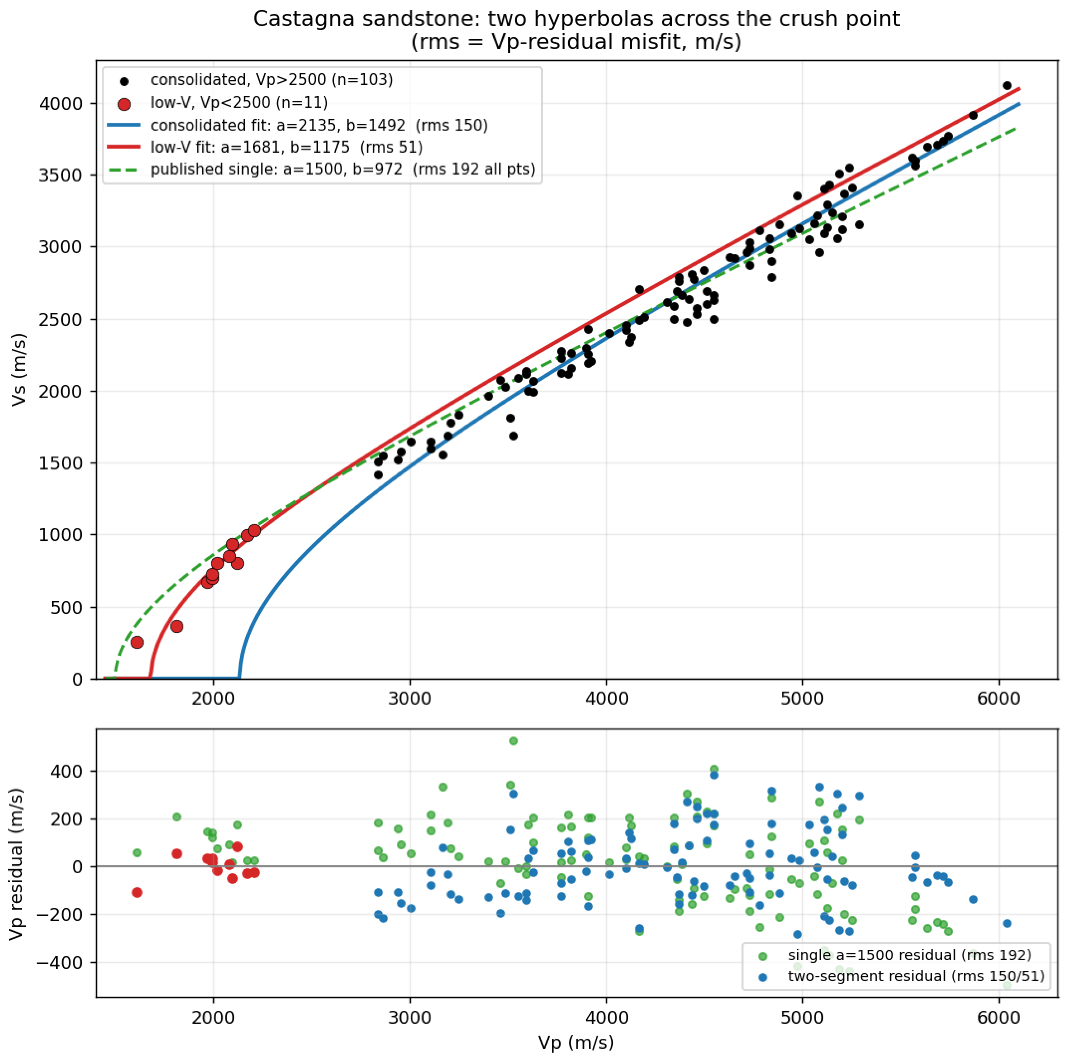
Qualification. The anchor is the worst-constrained quantity: the consolidated points sit well above the vertex, so reaching the Vs = 0 intercept is a long extrapolation, and two reasonable fitting choices span 2135–2245, so “~2200” is approximate. This is also a brine-saturated, mixed-provenance compilation; across plausible brines the anchor alone can move ~250 m/s. The direction (anchor well above 1500) is robust; the precise value is not.
E2. The Low-Velocity Segment
Fitting both parameters to the eleven points below 2500 m/s gives a = 1675, b = 1174, misfit 56. (These eleven points were independently re-digitized from Figure 4 to check the result below; the re-read reproduced the original fit, a = 1681, b = 1175, to within 6 m/s, misfit 51.) Despite the small sample the anchor is well determined — a bootstrap puts it at 1614–1771 — because these points sit on the vertex; the lowest, Vp = 1600, Vs = 250, is almost on the Vs = 0 axis and pins the intercept directly. The slope is the shaky parameter, b = 1174 with a bootstrap range of roughly 1100–1400.
So the data carry two distinct anchors, ~1680 and ~2135, whose bootstrap ranges do not overlap. That is the two-sided structure: a coherent Nur hyperbola on each side of the crush point rather than one curve spanning both, in sandstone as Higginbotham (2025) reports for shale.
The mechanism is a genuine flattening: the lowest-velocity points are Vs-deficient — they sit above Castagna’s linear fit (the two lowest by +231 and +295 m/s in Vp), which in this Vp-vertical plane is the shear-softening direction ϕs < ϕc predicts. They curve over toward a vertex near 1675, above where the straight line would cross Vs = 0 (1064 m/s). It is that curvature, not scatter, that the test in §E4 detects.
Qualifications. The eleven-point anchor leans on the two or three lowest points; they pin the vertex and carry the result, so the whole low-V segment rests on them. They have now been re-digitized independently and sit in the physically predicted direction, which is reassuring, but they remain the load-bearing data. The split at 2500 m/s was chosen, not detected — see §E4 for whether that split can manufacture the structure on its own. And the low-V anchor of ~1675 is only about one standard deviation above the 1500 m/s fluid value, so this side is barely distinguishable from a brine fluid. The low absolute misfit (56 versus 150) is partly the narrow Vp span of these points.
E3. Two Anchors, One Slope — Proportional Softening
The two segments share an asymptotic slope. From the hyperbola, which approaches a/b at high velocity, so a/b is the mineral-end the curve approaches; it depends only on K/μ, as does Poisson’s ratio. Both fits return a/b ≈ 1.43 despite anchors differing by 27%, and the two curves are related by a single scale:
| a | b | a/b | |
| consolidated | 2135 | 1492 | 1.431 |
| low-V (re-digitized) | 1681 | 1175 | 1.431 |
| ratio (low / consolidated) | 0.787 | 0.788 | — |
The a-ratio and b-ratio agree to ~0.0002: the low-velocity hyperbola is the consolidated one uniformly rescaled by ~0.79 in velocity — one curve shrunk, not two independent fits that happen to share a slope.
That is the signature of proportional softening across the crush point: if crossing it multiplies both K and μ by the same factor (here ~0.62, since velocity goes as the square root), K/μ is untouched, so Poisson’s ratio and the slope a/b are preserved while the overall stiffness — the anchor — drops. The crush point moves the vertex and leaves the slope alone. This stands cleanly against the paper’s central mechanism: approaching the bulk critical porosity, shear softens preferentially (ϕs < ϕc), which bends a/b below the mineral value near the vertex — a slope effect. Same data plane, two orthogonal fingerprints: the crush point slides the vertex at fixed slope; near-critical shear softening tilts the asymptote.
Qualifications. The slope is preserved exactly only if the softening factor is roughly uniform across the segment; a strongly porosity-dependent factor would tilt a/b, and the four-decimal b-ratio match rests on a poorly-constrained low-V slope (bootstrap a/b 1.27–1.52). Taken literally to ϕ = 0, ratio preservation would force the segments to share critical porosities; what the post-crush segment carries is its own apparent pair while sharing the high-velocity asymptote to the accuracy visible here. As a reading of why two anchors share a slope, proportional softening is the natural explanation, but it is an interpretation of an eleven-point fit.
E4. Is the Structure Real, or an Artifact of a Linear Trend?
Castagna fit these data with a single straight line, Vs = 0.8042 Vp − 0.8559, and the band does look linear — and the high-velocity arm of a hyperbola is nearly straight, so the worry is real: could splitting a fundamentally linear dataset at 2500 and fitting two hyperbolas manufacture both the two anchors and the shared slope? Two tests say no.
A noiseless version of Castagna’s line, sliced and fit the same way, gives the two halves very different slopes (a/b = 1.44 consolidated versus 1.91 for the low-V half) and unmatched ratios (0.65, 0.49) — qualitatively unlike the real data’s matched 1.431 / 1.431 and 0.787 / 0.788. A straight line does not share its slope across a split.
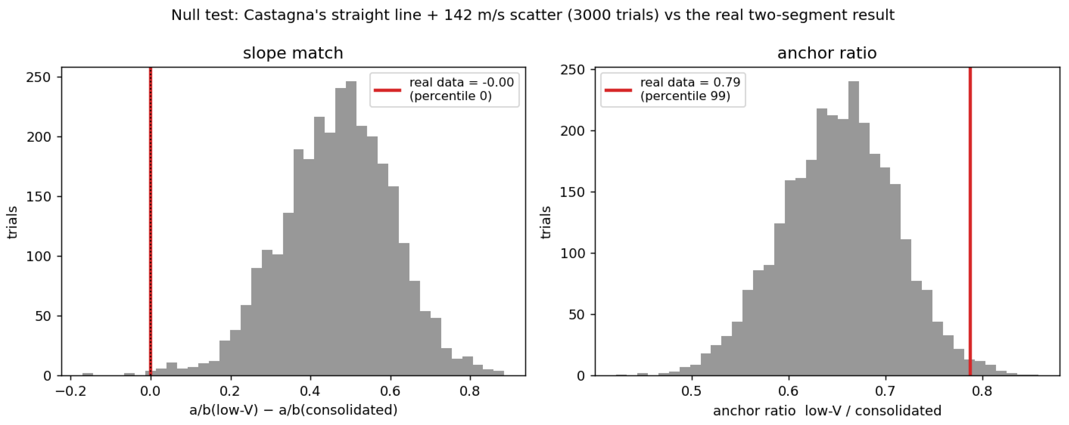
Adding scatter does not rescue the line. Drawing 3000 datasets as the line plus Gaussian noise matched to the real scatter about it (142 m/s), splitting and fitting each, the low-V half is always steeper: the slope difference a/b(low) − a/b(high) clusters at +0.47, and the real value (−0.0003) falls at percentile 0 — outside all 3000 trials (Figure E2). The anchor ratio sits at percentile 99. Crucially, the null uses the same split, so the split is exonerated as the source: what the line cannot reproduce is the low-velocity points bending over into a vertex that shares the consolidated slope. That bend is the Vs-deficiency of §E2, and it is what the re-digitization confirmed.
Qualifications. This rejects the single-line null — Castagna’s own model — not every conceivable alternative; a smoothly curving single trend was not tested as a null. The scatter was modeled as Gaussian and i.i.d. in Vp. And the percentile-0 signal is carried by the same two or three lowest points; it is robust to re-digitization and points the predicted way, but it is those points that make it.
Figure E2.
Null test. 3000 datasets drawn as Castagna’s straight line plus 142 m/s scatter, split and fit the same way. The line+scatter null never matches the two segments’ slopes (left, real value at percentile 0) and clusters the anchor ratio well below the data (right, real at percentile 99).
Figure E2.
Null test. 3000 datasets drawn as Castagna’s straight line plus 142 m/s scatter, split and fit the same way. The line+scatter null never matches the two segments’ slopes (left, real value at percentile 0) and clusters the anchor ratio well below the data (right, real at percentile 99).
E5. The Clean Check: Han Dry Frames
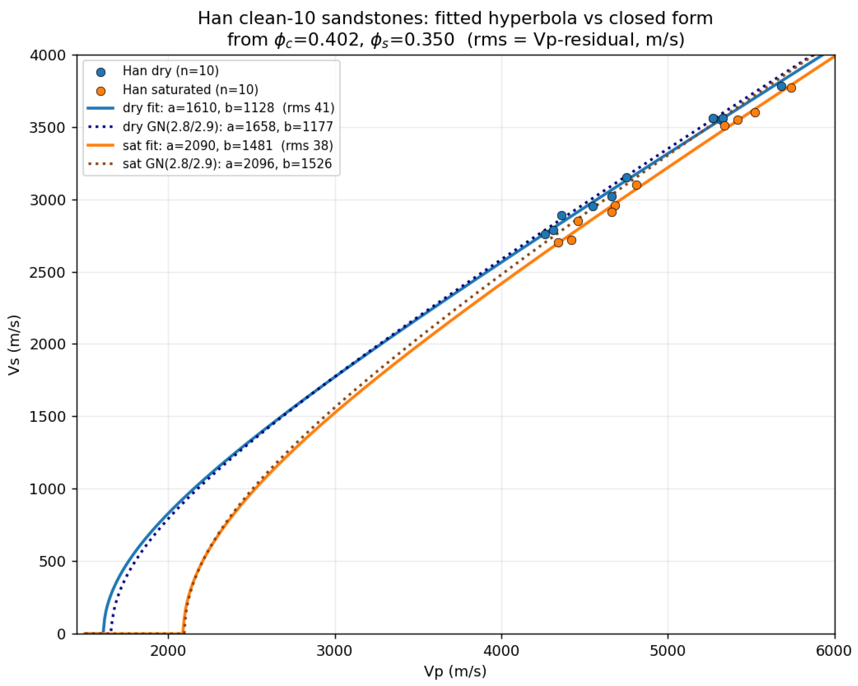
The Castagna compilation is digitized, fluid-mixed, and operator-split. The Han (1986) clean-10 sandstones are none of these: dry measurements, and ϕc = 0.402, ϕs = 0.350 already known from the moduli. Fitting the hyperbola directly to those ten samples and comparing with the closed forms (2.8)/(2.9) at those critical porosities:
| fitted a | fitted a/b | GN a (Km 36.6 / 40) | GN a/b (Km 36.6 / 40) | misfit | |
| dry | 1610 | 1.428 | 1658 / 1733 | 1.409 / 1.430 | 41 |
| saturated | 2090 | 1.411 | 2096 / 2150 | 1.374 / 1.396 | 38 |
The fit and the closed form agree (Figure E3). The saturated anchor is essentially exact against prediction; the dry anchor is within ~50 m/s and well inside its bootstrap band (1416–1795). The misfits, ~40 m/s, are five times tighter than Castagna’s 191. Three things follow.
The hyperbola the velocities trace is the one their own moduli predict — the closed-form machinery closes on real data. Qualification: ϕc and ϕs came from these same ten samples’ dry moduli, so this is an internal consistency check, not independent evidence for ϕs < ϕc beyond what the moduli already carry. It validates the algebra; it does not re-measure the separation.
The saturated Han anchor, ~2090, reproduces the Castagna consolidated anchor, ~2135 — two unrelated brine-saturated sandstone datasets agreeing. That part is independent, and it says the Castagna consolidated anchor is not a digitizing artifact.
The slope a/b sits below the quartz mineral value of 1.465 in both fluid states (1.43 dry, 1.41 saturated) — the ϕs < ϕc signature read off the asymptote. The dry-to-saturated anchor jump, 1610 → 2090, is the Gassmann fluid step (the ϕc → ϕc′ mapping), matching the predicted saturated value.
Qualification. The mineral modulus is not pinned: the anchor leans toward Km = 36.6 (true quartz) while the dry a/b leans toward Han’s Km = 40. The data cannot resolve it — the unreliable zero-porosity extrapolation — but either value brackets the fits closely, and nothing above turns on the choice.
Figure E3.
Han clean-10 sandstones, dry (blue) and saturated (orange). Solid curves are the free hyperbola fits; dotted curves are the closed forms (2.8)/(2.9) at the measured ϕc = 0.402, ϕs = 0.350. Fit and prediction overlie through the data. Legend misfits are RMS Vp residuals (m/s).
Figure E3.
Han clean-10 sandstones, dry (blue) and saturated (orange). Solid curves are the free hyperbola fits; dotted curves are the closed forms (2.8)/(2.9) at the measured ϕc = 0.402, ϕs = 0.350. Fit and prediction overlie through the data. Legend misfits are RMS Vp residuals (m/s).
E6. Three Softeners
The fits separate three ways a frame can lose stiffness, by what each does to the slope versus the anchor. Clay softens K and μ together — Poisson-preserving, an anchor shift at fixed slope (the §4.4 discriminant). The crush point, on this evidence, does the same: a proportional, Poisson-preserving step that drops the anchor and leaves a/b alone. Approaching the bulk critical porosity does the opposite — shear softens preferentially, tilting a/b below the mineral value while the anchor stays put. The first two slide the vertex; the third tilts the asymptote.
What this Does and Does Not Establish
It establishes that on the dataset where the critical porosities are known, the directly-fitted hyperbola matches the closed-form prediction in both fluid states; that the saturated anchor reproduces across two independent datasets; that the two Castagna segments are related by a single uniform rescaling, the signature of a proportional crush point; and that this two-segment structure is not an artifact of fitting hyperbolas to a linear trend — a straight line, with or without realistic scatter, cannot reproduce the shared slope (percentile 0).
It does not establish a discrete crush point as against smooth curvature — the split was imposed, and the null test rejects only the single-line alternative, not a smoothly curving one. It does not independently confirm ϕs < ϕc beyond the moduli; the Han hyperbola check is internal, with the saturated-anchor cross-match to Castagna the one genuinely independent piece. And the Castagna two-segment result, though it survives re-digitization and the line-null test, still rests on the two or three lowest-velocity points. The load-bearing evidence for the paper’s claim remains the dry Han frames of §4; these fits corroborate the picture and sharpen the distinction between the crush point (anchor shift, slope fixed) and the near-critical shear softening (slope tilt) without carrying the argument by themselves.
Appendix F. The Han (1986) Sandstone Data
The table reproduces the measured ultrasonic velocities, porosity, and clay content of the 69 sandstones underlying Section 4 and Section 5, as tabulated by Han (1986, pp. 159–161) at 40 MPa confining pressure and 1 MPa pore pressure, the saturated state being full saturation with deionized water. These are Han’s measurements, transcribed here for reference, not quantities computed in the present work. Velocities are in km/s; porosity and clay fraction are dimensionless. The 10 clay-free samples (clay < 0.025), listed first, are the clean-ten of §4.
| Sample | Porosity | Clay | Vp dry | Vs dry | Vp sat | Vs sat |
| FONT D | 0.055 | 0.000 | 5.68 | 3.78 | 5.74 | 3.77 |
| BEAVER | 0.064 | 0.000 | 5.27 | 3.56 | 5.52 | 3.60 |
| FONT C | 0.075 | 0.000 | 5.32 | 3.55 | 5.42 | 3.55 |
| FONT E | 0.097 | 0.000 | 5.33 | 3.56 | 5.34 | 3.51 |
| FONT A | 0.154 | 0.000 | 4.75 | 3.15 | 4.81 | 3.10 |
| FONT G | 0.177 | 0.000 | 4.66 | 3.02 | 4.68 | 2.96 |
| PETERA | 0.182 | 0.000 | 4.55 | 2.95 | 4.66 | 2.91 |
| FONT B | 0.197 | 0.000 | 4.36 | 2.89 | 4.46 | 2.85 |
| PETERC | 0.199 | 0.000 | 4.31 | 2.79 | 4.42 | 2.72 |
| FONT H | 0.224 | 0.000 | 4.26 | 2.76 | 4.34 | 2.70 |
| DETANBUF | 0.155 | 0.030 | 4.61 | 3.01 | 4.60 | 2.81 |
| BEREA4 | 0.216 | 0.030 | 3.84 | 2.50 | 3.95 | 2.39 |
| MASSBURG | 0.237 | 0.030 | 3.82 | 2.48 | 3.89 | 2.37 |
| MASSILIA | 0.207 | 0.040 | 3.92 | 2.51 | 4.03 | 2.40 |
| CONATTON | 0.230 | 0.040 | 3.81 | 2.49 | 3.92 | 2.35 |
| DELBROWN | 0.106 | 0.050 | 4.47 | 2.92 | 4.73 | 2.89 |
| UNH1 | 0.188 | 0.050 | 4.14 | 2.64 | 4.18 | 2.50 |
| UTAHBUFF | 0.057 | 0.060 | 4.80 | 3.21 | 4.94 | 3.12 |
| COCONINO | 0.106 | 0.060 | 4.69 | 3.07 | 4.73 | 3.00 |
| G-15879 | 0.151 | 0.060 | 4.35 | 2.73 | 4.61 | 2.73 |
| MASSDARK | 0.176 | 0.060 | 4.22 | 2.71 | 4.32 | 2.62 |
| MASDARK1 | 0.181 | 0.060 | 4.20 | 2.69 | 4.30 | 2.57 |
| BEREA1 | 0.190 | 0.060 | 4.04 | 2.62 | 4.15 | 2.51 |
| BEREA35 | 0.221 | 0.060 | 3.91 | 2.49 | 4.03 | 2.40 |
| BOISE | 0.254 | 0.060 | 3.61 | 2.20 | 3.74 | 2.08 |
| G-12674 | 0.268 | 0.060 | 3.52 | 2.24 | 3.61 | 2.09 |
| DLITGRY | 0.041 | 0.070 | 4.94 | 3.16 | 5.20 | 3.17 |
| G-12677 | 0.266 | 0.070 | 3.41 | 2.15 | 3.50 | 1.99 |
| G-12677B | 0.274 | 0.070 | 3.44 | 2.21 | 3.59 | 2.09 |
| NUGGETV | 0.091 | 0.080 | 4.48 | 3.01 | 4.69 | 2.94 |
| NUGGETH | 0.092 | 0.080 | 4.74 | 3.12 | 4.88 | 3.05 |
| G-12670 | 0.263 | 0.080 | 3.57 | 2.32 | 3.67 | 2.20 |
| BEREA5 | 0.189 | 0.090 | 3.99 | 2.63 | 4.08 | 2.54 |
| P74-8797 | 0.156 | 0.100 | 4.11 | 2.63 | 4.24 | 2.51 |
| IDLIGHT | 0.235 | 0.100 | 3.65 | 2.36 | 3.68 | 2.22 |
| IDLIGHT1 | 0.240 | 0.100 | 3.54 | 2.28 | 3.69 | 2.17 |
| P82-7377 | 0.173 | 0.110 | 4.17 | 2.61 | 4.23 | 2.43 |
| G-14807 | 0.202 | 0.110 | 3.71 | 2.33 | 3.88 | 2.23 |
| G-12676 | 0.279 | 0.110 | 3.45 | 2.20 | 3.56 | 2.07 |
| G-10431 | 0.299 | 0.110 | 3.09 | 1.91 | 3.20 | 1.75 |
| G-12416 | 0.253 | 0.120 | 3.41 | 2.13 | 3.55 | 1.94 |
| G-10432 | 0.294 | 0.120 | 3.03 | 1.92 | 3.17 | 1.77 |
| P64-6264 | 0.140 | 0.130 | 4.24 | 2.72 | 4.47 | 2.64 |
| TORY-AV | 0.131 | 0.140 | 4.06 | 2.62 | 4.23 | 2.41 |
| P72-7154 | 0.163 | 0.140 | 4.16 | 2.71 | 4.32 | 2.55 |
| P82-7379 | 0.170 | 0.160 | 4.11 | 2.63 | 4.19 | 2.42 |
| INDDARK1 | 0.256 | 0.160 | 3.46 | 2.21 | 3.54 | 2.05 |
| IDDARK | 0.260 | 0.160 | 3.27 | 2.15 | 3.36 | 1.99 |
| G-15949 | 0.144 | 0.180 | 3.78 | 2.32 | 4.07 | 2.37 |
| G-15845 | 0.109 | 0.210 | 3.86 | 2.47 | 4.25 | 2.48 |
| G-12415 | 0.243 | 0.220 | 3.27 | 2.09 | 3.36 | 1.89 |
| G-15858 | 0.102 | 0.230 | 3.99 | 2.60 | 4.42 | 2.61 |
| G-15930 | 0.059 | 0.240 | 3.65 | 2.51 | 4.60 | 2.77 |
| SANTABAR | 0.126 | 0.270 | 3.75 | 2.36 | 4.06 | 2.24 |
| G-12660H | 0.143 | 0.270 | 3.59 | 2.18 | 3.98 | 2.19 |
| G-12409B | 0.145 | 0.270 | 3.49 | 2.19 | 4.00 | 2.16 |
| REDSTONE | 0.159 | 0.280 | 3.54 | 2.09 | 3.82 | 2.07 |
| P64-6258 | 0.093 | 0.350 | 3.97 | 2.70 | 4.17 | 2.43 |
| P63-6254 | 0.112 | 0.370 | 3.92 | 2.56 | 4.08 | 2.34 |
| G-12418 | 0.143 | 0.370 | 3.23 | 2.12 | 3.76 | 2.11 |
| P61-5561 | 0.063 | 0.380 | 4.11 | 2.78 | 4.37 | 2.62 |
| P63-6249 | 0.072 | 0.400 | 4.06 | 2.72 | 4.24 | 2.49 |
| P64-6256 | 0.088 | 0.400 | 4.02 | 2.65 | 4.24 | 2.52 |
| G-10452 | 0.094 | 0.410 | 3.32 | 2.21 | 3.97 | 2.19 |
| G-12425 | 0.109 | 0.440 | 3.41 | 2.23 | 3.84 | 2.15 |
| G-10379 | 0.128 | 0.440 | 3.33 | 2.14 | 3.71 | 1.97 |
| P64-6260 | 0.068 | 0.450 | 4.06 | 2.77 | 4.32 | 2.57 |
| G-10381 | 0.131 | 0.460 | 3.19 | 2.10 | 3.63 | 1.99 |
| G-10392 | 0.115 | 0.510 | 3.10 | 2.02 | 3.68 | 2.01 |
Appendix G. The Dry-Frame Regression of §4.1 and §4.2
Section 4.1 and Section 4.2 compress a short chain of standard estimation steps into two displayed results, (4.2) and the critical porosities that follow from it. This appendix sets out that chain, since the error bars quoted in §4.2 depend on a covariance term that is easy to omit and that changes them by roughly a factor of two.
G1. From Tabulated Velocities to Dry-Frame Moduli
The inputs are the dry velocities and porosities of Appendix F, measured at 40 MPa confining and 1 MPa pore pressure. The clean subset is taken as the clay-free samples, ten in number, spanning . Equation (4.1) converts each triplet into a pair of dry-frame moduli using the dry density with g/cm³. No fluid modulus and no fluid density enter at any point, which is the sense in which the determination is frequency-robust (§4.1): the quantities regressed are frame properties, not Gassmann-substituted ones.
G2. The Straight-Line Fit
Each modulus is regressed on porosity in the critical-porosity form (3.1), a two-parameter linear model
fitted by ordinary least squares. With the design matrix , the coefficients and their joint uncertainty are
where RSS is the residual sum of squares and the degrees of freedom. The square roots of the diagonal of are the coefficient uncertainties quoted in (4.2); the off-diagonal element is used in §G3. Numerically,
| intercept (GPa) | slope (GPa) | (GPa) | ||
| 1.56 | ||||
| 1.12 |
G3. The Critical Porosities and Their Uncertainty
Each critical porosity is the zero crossing of its fitted line,
a ratio of two correlated estimates. Propagating to first order (the delta method) gives
which yields the values quoted in §4.2, and .
The covariance term is not a refinement. Because the measured porosities lie well away from , the intercept and slope are strongly anti-correlated: a fit passing higher at the origin must descend more steeply to reach the same data. Their errors therefore partly cancel in the ratio (G.3), and the line’s zero crossing is far better determined than either coefficient alone. Dropping the third term of (G.4) inflates the uncertainties to and — nearly double, and a needlessly pessimistic reading of the same fit.
The correlation itself is a property of the design rather than of the data: since is times a matrix built only from the porosities, the scale factor cancels in the correlation, and the bulk and shear fits share the identical value . What differs between them is only the overall scale .
G4. Why the Shear Critical Porosity is the Better Determined of the Two
Two effects compound. The shear fit is the tighter of the pair, against GPa, a ratio of 1.39; and its zero crossing lies nearer the data, requiring extrapolation from out to 0.350 rather than to 0.402. A shorter reach on a tighter line gives the factor of roughly two separating from .
G5. The Separation and its Significance
The quantity of interest is the difference
whose uncertainty §4.2 quotes as . That figure combines the two individual uncertainties as though the fits were independent. They are not: a sample that is stiff in bulk is generally stiff in shear, and the residuals of the two fits correlate sample-by-sample at . A paired resampling that preserves that correlation — refitting both moduli on the same bootstrap draws — gives , with the separation positive in essentially every resample.
The two estimates bracket the claim made in §4.2. Independent propagation gives 1.9 standard errors, the paired bootstrap 2.9; the text’s “two-to-three sigma” spans both, and the published is the conservative choice. Given ten samples, the bootstrap figure is the more optimistic of the two and is reported here for completeness rather than substituted for the analytic one.
G6. Robustness of the Separation
Because the zero crossings are extrapolations, the lowest-porosity frames carry the most leverage, and the separation was checked against their influence. Refitting with each sample deleted in turn changes by at most 0.017 — the largest single shift, , on removal of the lowest-porosity frame (FONT D, ), and the largest downward shift, , on removal of BEAVER (). Removing the lowest-porosity frames cumulatively rather than singly leaves between 0.050 and 0.069 as the first three are dropped. The separation is positive in every such subset.
G7. What these Uncertainties do and do not Cover
The intervals of §G3 and §G5 are the classical least-squares intervals, and they assume residuals that are independent with constant variance and, critically, a linear modulus–porosity relation that holds out to the zero crossing. The first two assumptions are unremarkable for this suite. The third is an extrapolation: the highest measured porosity is 0.224, and both critical porosities lie beyond it, so the quoted intervals measure scatter about the fitted lines and not the risk that the frame ceases to be linear somewhere between the last datum and the intercept. That risk is not quantified by any resampling of these ten points, since every resample inherits the same porosity range.
This is the reason §4.3 carries more weight than §4.2. The rise of across the measured range is a statement about the interval in which the data actually lie, and it rejects the constant-Poisson idealization without extrapolating at all.
References
- Aplin, A. C. Assessment of. β, the compression coefficient of mudstones and its relationship with detailed lithology: Marine and Petroleum Geology 1995, 12(no. 8), 955–963. [Google Scholar] [CrossRef]
- Bachrach, R.; Avseth, P. Rock physics modeling of unconsolidated sands: Accounting for nonuniform contacts and heterogeneous stress fields in the effective media approximation with applications to hydrocarbon exploration. Geophysics 2008, 73(no. 6), E197–E209. [Google Scholar] [CrossRef]
- Batzle, M.; Wang, Z. Seismic properties of pore fluids. Geophysics 1992, 57(no. 11), 1396–1408. [Google Scholar] [CrossRef]
- Castagna, J. P.; Batzle, M. L.; Kan, T. K. Rock physics — The link between rock properties and AVO response. In Offset-dependent reflectivity — Theory and practice of AVO analysis: Society of Exploration Geophysicists, Investigations in Geophysics; Castagna, J. P., Backus, M. M., Eds.; 1993; Volume 8, pp. 135–171. [Google Scholar]
- Gomez, C. T.; Dvorkin, J.; Vanorio, T. Laboratory measurements of porosity, permeability, resistivity, and velocity on Fontainebleau sandstones. Geophysics 2010, 75(no. 6), E191–E204. [Google Scholar] [CrossRef]
- Hamilton, E. L. Shear-wave velocity versus depth in marine sediments: A review. Geophysics 1976, 41(no. 5), 985–996. [Google Scholar] [CrossRef]
- Han, D.-H. Effects of porosity and clay content on acoustic properties of sandstones and unconsolidated sediments. Ph.D. dissertation, Stanford University, 1986. [Google Scholar]
- Higginbotham, J.; Brown, M. P.; Ramirez, O. Amplitude calibration: SEG Technical Program Expanded Abstracts 2011, 365–369.
- Higginbotham, J.; Macesanu, C.; Brown, M. P.; Ramirez, O.; Joanne, C. An alternative amplitude analysis theory: SEG Technical Program Expanded Abstracts. 2012. [Google Scholar] [CrossRef] [PubMed]
- Higginbotham, J. Gassmann–Nur–Aplin pore pressure prediction: SEG Technical Program Expanded Abstracts. 2020, 2211–2215. [Google Scholar] [CrossRef]
- Higginbotham, J. An interpretation of Gardner’s equation. Innovative Journal of Applied Science 2025, 2(no. 5), 37. [Google Scholar] [CrossRef]
- Ji, S.; Li, L.; Motra, H. B.; Wuttke, F.; Sun, S.; Michibayashi, K.; Salisbury, M. H. Poisson’s ratio and auxetic properties of natural rocks. Journal of Geophysical Research: Solid Earth 2018, 123(no. 2), 1161–1185. [Google Scholar] [CrossRef]
- Krief, M.; Garat, J.; Stellingwerff, J.; Ventre, J. A petrophysical interpretation using the velocities of P and S waves (full-waveform sonic): The Log Analyst. 1990, 31, 355–369. [Google Scholar]
- Liu, A. J.; Nagel, S. R. The jamming transition and the marginally jammed solid. Annual Review of Condensed Matter Physics 2010, 1, 347–369. [Google Scholar] [CrossRef]
- Makse, H. A.; Johnson, D. L.; Schwartz, L. M. Packing of compressible granular materials. Physical Review Letters 2000, 84, 4160–4163. [Google Scholar] [CrossRef] [PubMed]
- Mavko, G.; Mukerji, T. Comparison of Krief and critical porosity models for prediction of porosity and Vp/Vs. Geophysics 1998, 63(no. 3), 925–927. [Google Scholar] [CrossRef]
- Mindlin, R. D. Compliance of elastic bodies in contact. Journal of Applied Mechanics 1949, 16, 259–268. [Google Scholar] [CrossRef]
- Mondol, N. H.; Jahren, J.; Bjørlykke, K.; Brevik, I. Elastic properties of clay minerals: The Leading Edge 2008, 27(no. 6), 758–770. [CrossRef]
- Nur, A.; Mavko, G.; Dvorkin, J.; Galmudi, D. Critical porosity: A key to relating physical properties to porosity in rocks: The Leading Edge. 1998, 17(no. 3), 357–362. [Google Scholar] [CrossRef]
- O’Hern, C. S.; Silbert, L. E.; Liu, A. J.; Nagel, S. R. Jamming at zero temperature and zero applied stress: The epitome of disorder. Physical Review E 2003, 68, 011306. [Google Scholar] [CrossRef]
- Sayers, C. M. Critical porosity and the elastic properties of reservoir rocks: The Leading Edge. 2025, 44(no. 6), 436–440. [Google Scholar] [CrossRef]
- Vernik, L.; Kachanov, M. Modeling elastic properties of siliciclastic rocks. Geophysics 2010a, 75(no. 6), E171–E182. [Google Scholar] [CrossRef]
- Vernik, L.; Kachanov, M. Modeling elastic properties of sands and sandstones: SEG Technical Program Expanded Abstracts 2010b, 2411–2415. [CrossRef]
- Zimmer, M. A. Seismic velocities in unconsolidated sands: Measurements of pressure, sorting, and compaction effects. Ph.D. dissertation, Stanford University, 2003. [Google Scholar]
Figure 1.
Compressional and shear velocities of sandstones (data: Castagna et al., 1993, pp. 138–139) trace the Gassmann–Nur hyperbola (2.4). The curve is the single-parameter fit of Higginbotham et al. (2011): the anchor is held at a brine pore fluid velocity a = 1500 m/s and only b = 972 m/s is adjusted, with a root-mean-square misfit of 191 m/s across the full range. The anchor a = 1500 m/s is the equal critical porosity special case (§2.4, §2.5 and equation (2.15) ); §2.2 shows the hyperbolic form exists for any constant pair (ϕc, ϕs). Similar plots for other minerals may be found in Higginbotham (2025) supplemental information.
Figure 1.
Compressional and shear velocities of sandstones (data: Castagna et al., 1993, pp. 138–139) trace the Gassmann–Nur hyperbola (2.4). The curve is the single-parameter fit of Higginbotham et al. (2011): the anchor is held at a brine pore fluid velocity a = 1500 m/s and only b = 972 m/s is adjusted, with a root-mean-square misfit of 191 m/s across the full range. The anchor a = 1500 m/s is the equal critical porosity special case (§2.4, §2.5 and equation (2.15) ); §2.2 shows the hyperbolic form exists for any constant pair (ϕc, ϕs). Similar plots for other minerals may be found in Higginbotham (2025) supplemental information.
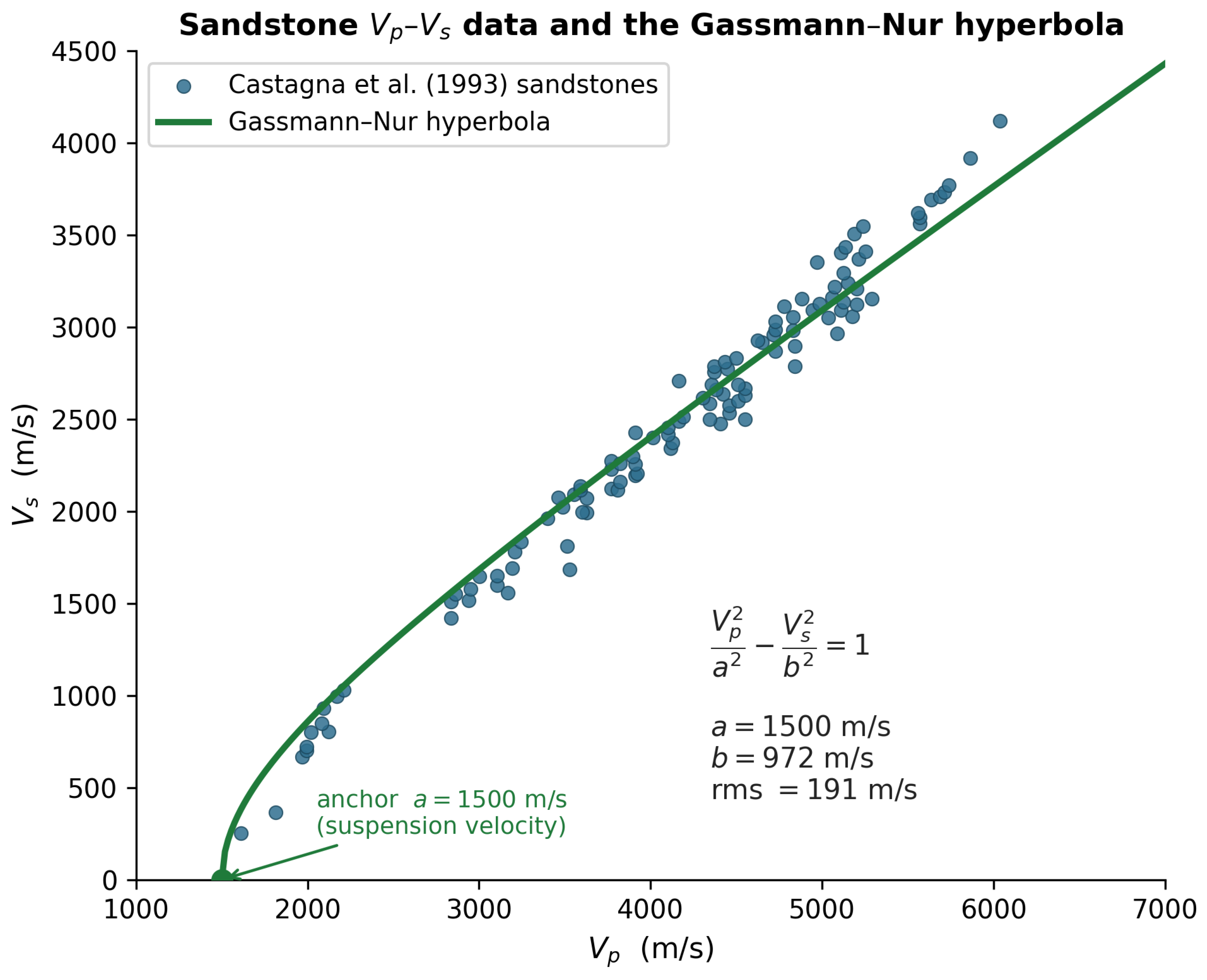
Figure 2.
Dry-frame bulk and shear moduli of the ten clean (clay < 0.025) Han (1986) quartz sandstones against porosity, with the least-squares lines (4.2). The shear modulus μd extrapolates to zero at ϕs = 0.350, below the bulk modulus Kd at ϕc = 0.402; the shaded band ϕs < ϕ < ϕc is the interval over which the dry frame carries compressional stiffness but no shear. Solid line segments span the measured porosities; the crossings are essentially extrapolations where points for both the shear modulus and the bulk modulus cluster (§4.2).
Figure 2.
Dry-frame bulk and shear moduli of the ten clean (clay < 0.025) Han (1986) quartz sandstones against porosity, with the least-squares lines (4.2). The shear modulus μd extrapolates to zero at ϕs = 0.350, below the bulk modulus Kd at ϕc = 0.402; the shaded band ϕs < ϕ < ϕc is the interval over which the dry frame carries compressional stiffness but no shear. Solid line segments span the measured porosities; the crossings are essentially extrapolations where points for both the shear modulus and the bulk modulus cluster (§4.2).
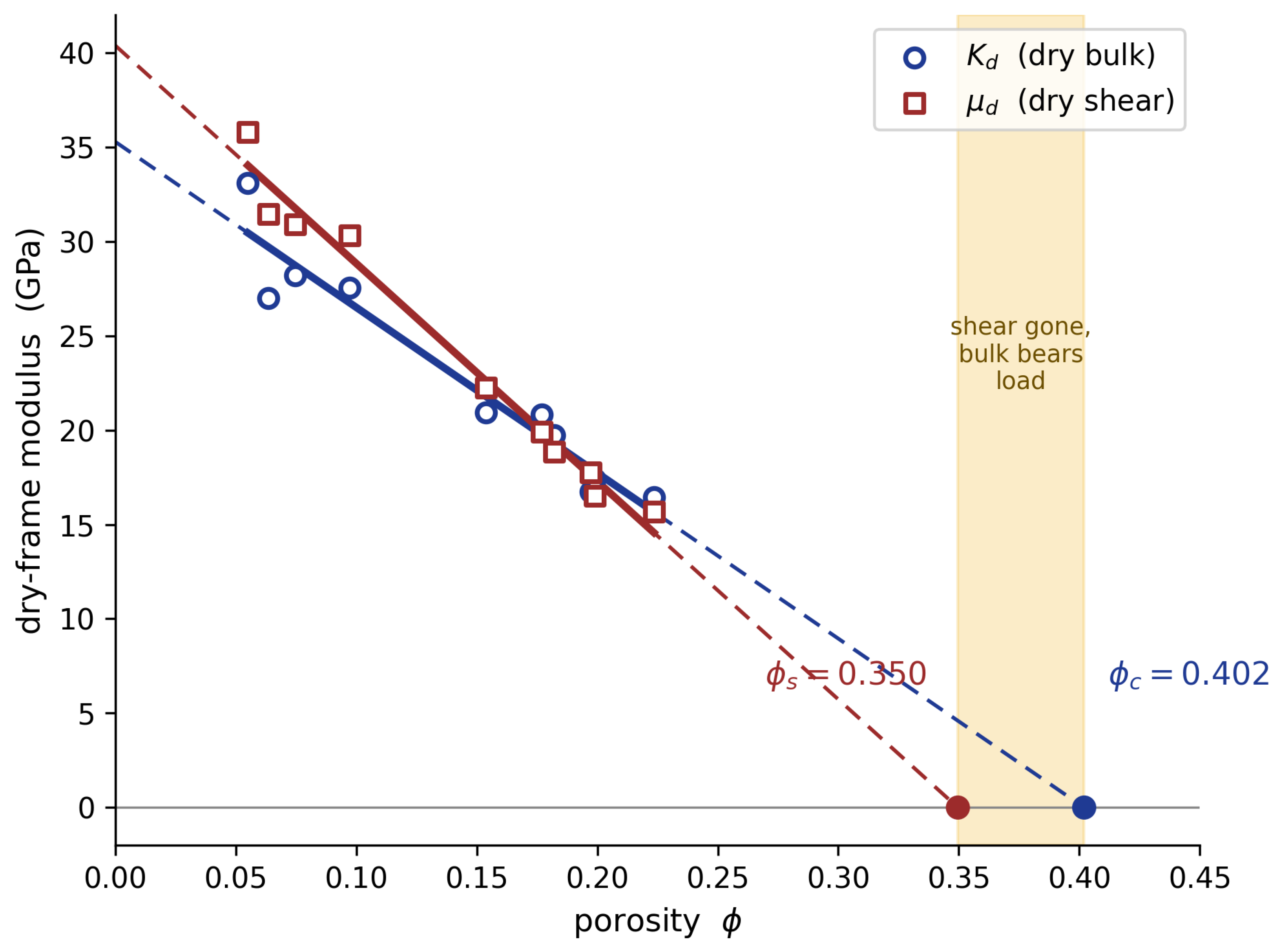
Disclaimer/Publisher’s Note: The statements, opinions and data contained in all publications are solely those of the individual author(s) and contributor(s) and not of MDPI and/or the editor(s). MDPI and/or the editor(s) disclaim responsibility for any injury to people or property resulting from any ideas, methods, instructions or products referred to in the content. |
© 2026 by the author. Licensee MDPI, Basel, Switzerland. This article is an open access article distributed under the terms and conditions of the Creative Commons Attribution (CC BY) license.
Copyright: This open access article is published under a Creative Commons CC BY 4.0 license, which permit the free download, distribution, and reuse, provided that the author and preprint are cited in any reuse.


