
Submitted:
30 June 2026
Posted:
01 July 2026
You are already at the latest version
Abstract
Variations in goaf temperature and CO concentration during the low-temperature oxidation stage are affected by residual-coal oxidation, air-leakage oxygen supply, gas generation, migration and dilution, and ventilation disturbance, leading to multi-source coupling and nonlinear response characteristics. To continuously characterize this process, this study proposes a joint prediction method for goaf temperature and CO concentration based on multi-source monitoring feature fusion and Covariance-Adaptive Whale Optimization Algorithm (CA-WOA)-optimized models. Field monitoring data, including goaf-pipe gas, working-face-side gas, upper-corner gas, and return-air-side gas, were integrated to construct a daily-scale multi-source monitoring dataset. Pearson correlation analysis and random forest-based feature importance ranking were combined to identify dominant variables and construct top-k feature subsets. CA-WOA was then developed from the original Whale Optimization Algorithm by incorporating rank-weighted elite-center reconstruction, covariance-adaptive direction learning, WOA random-search injection, and geometric step-size decay. A composite normalized error of temperature and CO concentration was used as the fitness function to optimize the hyperparameters of RF, XGBoost, LightGBM, CatBoost, LSSVM, and TABM under a unified evaluation criterion. The results show that CA-WOA improved the overall predictive performance of all six models. Compared with the corresponding unoptimized baselines, the maximum increase in Mean R² was 0.076, and the maximum reduction in the composite fitness F was 22.8%. CA-WOA-TABM achieved the best performance, with a five-fold average Mean R² of 0.924 and F of 0.273. Its out-of-fold R² values for temperature and CO concentration were 0.928 and 0.931, respectively, demonstrating stable internal validation performance. SHAP and PDP analyses identified GoafPipe_CH4, GoafPipe_CO2, GoafPipe_C2H6, and GoafPipe_O2 as key variables, indicating nonlinear response relationships associated with gas generation, oxygen supply, and gas migration in the goaf during continuous monitoring.
Keywords:
goaf
; low-temperature oxidation
; multi-source monitoring
; joint prediction of temperature and CO concentration
; covariance-adaptive whale optimization algorithm
; TABM
; SHAP/PDP
1. Introduction
Coal remains a fundamental energy source in the global energy supply system and plays a crucial role in China’s energy security. Despite the rapid development of renewable energy, coal is still indispensable for electricity generation, industrial production, and basic energy supply [1]. Mine fires are a major threat to coal mine safety, and coal spontaneous combustion is one of their principal causes. Some statistics indicate that coal spontaneous combustion accounts for approximately 90% of mine fire events, leading to resource losses, production interruption, and secondary hazards such as gas explosions [2]. As mining depth increases, the occurrence of residual coal, air-leakage oxygen supply, and heat accumulation in goafs becomes more complex, thereby increasing the uncertainty of internal temperature evolution and gas migration processes [3]. In an actual working-face goaf, monitoring points such as goaf pipes, upper corners, return-air sides, and working-face sides reflect different aspects of the system. Therefore, a single monitoring point or gas indicator is insufficient to fully characterize the low-temperature oxidation state, and multi-source monitoring information is required to jointly describe oxidation-related gas generation and thermal evolution in the goaf [4].
The low-temperature oxidation mechanism of coal spontaneous combustion provides the basis for selecting monitoring indicators and evaluating coal temperature. Anghelescu et al. [2] and Liu et al. [5] reported that exothermic low-temperature oxidation caused by coal–oxygen interaction is the core process underlying the incubation of coal spontaneous combustion. A rise in temperature further accelerates oxidation reactions and promotes heat accumulation. Ma et al. [6] combined programmed heating with Fourier-transform infrared spectroscopy (FTIR) to analyze gas-release differences at different oxidation stages and suggested that CO, C2H4, and the Graham coefficient can serve as important discriminant indicators. Liu et al. [7] used wavelet analysis to reveal the multi-scale evolution of CO and O2 volume fractions in different areas of a working face. These studies show that O2, CO, CO2, and hydrocarbon gases can reflect the degree of coal oxidation; however, their responses are jointly affected by coal quality, oxygen supply, temperature stage, and sampling location [8].
Goaf coal spontaneous combustion differs from the oxidation of a single coal sample. Its occurrence and development are controlled by residual-coal distribution, air-leakage oxygen supply, overburden fractures, heat accumulation, and ventilation boundaries [3]. Zhang et al. [9] pointed out that multi-factor coupled hazards become more prominent under deep mining conditions, and monitoring-based identification should develop toward spatiotemporal, multi-scale, and multi-parameter approaches. Jin et al. [10] summarized the insufficient field observability and spatial inversion difficulties associated with hidden fire-source localization. Zhai et al. [11] revised the relationship between CO and coal temperature under air-leakage conditions and established a corresponding discrimination method. These findings indicate that the low-temperature oxidation state of a goaf is not directly determined by a single gas indicator. Instead, it is jointly shaped by oxygen supply, oxidation heat release, gas generation, air-leakage dilution, and migration lag. Consequently, variations in temperature and CO concentration depend more strongly on the joint characterization of multi-source information [5].
Traditional discrimination methods for coal spontaneous combustion mainly rely on indicator gases, composite gas ratios, critical temperatures, and empirical thresholds. A previous study [12], Hao et al. [13], and Zhang et al. [14] developed discrimination criteria based on composite gas characteristics, the Graham coefficient, and multi-indicator collaborative analysis. Wang et al. [15] and Zhongyu et al. [16] further improved traditional methods by analyzing CO source identification and gas–temperature statistical relationships. These methods have clear physical meanings and are convenient for engineering deployment. However, under air-leakage dilution, gas-response lag, multi-point differences, and spatial coupling, fixed thresholds are difficult to use for a stable description of the continuous evolution process during the low-temperature oxidation stage [11].
With the accumulation of mine monitoring data, machine learning methods have increasingly been applied to coal temperature prediction and coal spontaneous combustion state identification. Wang et al. [16] developed a BPNN model based on gas composition, spatial distance, and coal temperature data for spatiotemporal temperature prediction. Lei et al. [8] established an RF model using programmed-heating data from coal samples collected from 12 coal mines and compared it with GBM, BPNN, and KNN, confirming the effectiveness of multi-indicator gases for coal temperature prediction. Zhuo et al. [17] and Zou et al. [18] applied PSO-XGBoost to coal temperature or spontaneous combustion tendency prediction, indicating that swarm-intelligence optimization can improve parameter selection and model accuracy. Guo et al. [19] combined PSO with GRU for coal temperature inversion in concealed spaces, enhancing the nonlinear mapping from gas indicators to coal temperature. For state identification, Zhang et al. [20] used t-SNE and k-means for coal spontaneous combustion state classification. Li et al. [21] constructed an NSGA-II-RF prediction model. Long et al. [22] applied BO-LightGBM for coal temperature prediction and state discrimination. Pan et al. [23] represented gas associations through GCN, while Zhao et al. [24] and Liu et al. [25] improved model generalization and joint identification from the perspectives of ensemble modeling and multi-task learning, respectively. Overall, existing studies have promoted the transition of coal spontaneous combustion monitoring from empirical thresholds to data-driven methods. Nevertheless, many studies are still oriented toward coal-sample experiments or general goaf scenarios. The fusion of multi-source information, including goaf-pipe gas, working-face gas, upper-corner gas, return-air-side gas, and ventilation disturbance, remains insufficient. In addition, most studies focus on single coal temperature prediction or state classification, while less attention has been paid to the continuous joint prediction of temperature and CO concentration during the low-temperature oxidation stage.
To address these issues, this study focuses on the low-temperature oxidation stage of a working-face goaf and proposes a joint prediction method for temperature and CO concentration based on multi-source monitoring feature fusion and CA-WOA-TABM. First, multi-source monitoring variables, including goaf-pipe gas, working-face-side gas, upper-corner gas, and return-air-side gas, are integrated to construct a daily-scale sample system. Correlation analysis and tree-model feature importance are then combined to select dominant features. Second, a Covariance-Adaptive Whale Optimization Algorithm (CA-WOA) is developed from the original WOA. Through rank-weighted elite-center reconstruction, covariance-adaptive direction learning, WOA random-search injection, and geometric step-size decay, the search stability in complex hyperparameter spaces is improved. The composite normalized error of temperature and CO concentration is used as the optimization objective to adaptively optimize six candidate regression models. Finally, SHAP and PDP methods are used to interpret the contribution magnitude, effect direction, and response ranges of key gas indicators for the dual-output prediction results, providing data-driven support for continuous characterization of the low-temperature oxidation state of the goaf.
2. Models and Methods
2.1. Overall Framework
This study constructs a joint prediction framework based on multi-source monitoring feature fusion and CA-WOA-TABM for the continuous prediction of goaf temperature and CO concentration during the low-temperature oxidation stage. As shown in Figure 1, the overall workflow consists of five components: data preprocessing, key feature screening, CA-WOA-based hyperparameter optimization, dual-output prediction using candidate regression models, and SHAP/PDP interpretation. The framework takes multi-source monitoring data as input and uses goaf temperature and CO concentration as dual-output targets, thereby characterizing the low-temperature oxidation process from the perspectives of thermal-state evolution and gas-generation response.
In the data preprocessing stage, variables related to goaf-pipe gas, upper-corner gas, return-air-side gas, working-face-side gas, and ventilation disturbance are organized in a unified manner. Outlier identification, missing-value imputation, temporal alignment, daily-scale aggregation, and robust standardization are then performed sequentially to form a daily-scale multi-source monitoring dataset. The model outputs are defined as goaf temperature and CO concentration. Temperature is used to characterize the evolution of the goaf thermal state, whereas CO concentration reflects the gas-generation response during low-temperature oxidation [26]. Because the monitoring period mainly corresponds to the low-temperature oxidation stage, this study does not construct a multi-level early-warning classification model but focuses on continuous prediction.
In the feature screening stage, correlation analysis and tree-model importance evaluation are combined to identify key variables. Correlation analysis is used to describe statistical associations between monitoring variables and prediction targets, whereas random forest-based feature importance is used to evaluate the nonlinear contribution of variables to the dual-output task. Based on the integrated importance ranking, different top-k feature subsets are constructed and separately input into six candidate regression models, namely RF, XGBoost, LightGBM, CatBoost, LSSVM, and TABM. This procedure aims to determine a compact feature combination that balances prediction accuracy, model complexity, and interpretability.
In the model optimization stage, CA-WOA is introduced to optimize the key hyperparameters of the six candidate regression models. The composite normalized error of temperature and CO concentration is used as a unified fitness function, enabling the parameter search to account for both output targets simultaneously and reducing the risk of optimizing the model toward only one variable. After optimization, all models are evaluated using the same feature subset and evaluation criteria under five-fold cross-validation, and out-of-fold predictions are used to assess internal validation stability.
In the interpretation stage, SHAP and PDP methods are applied to the better-performing models. SHAP quantifies the global contribution and local effects of key monitoring variables on temperature and CO predictions, whereas PDP analyzes the marginal response trends of model outputs as important variables and their combinations vary. Through this workflow, the study establishes a complete modeling chain from multi-source monitoring data fusion, key feature screening, and adaptive hyperparameter optimization to model interpretation, providing a data-driven method for the continuous characterization of the low-temperature oxidation state of the goaf.
2.2. Dominant Feature Selection Method
Multi-source monitoring variables are collected from different spatial locations, including goaf pipes, upper corners, return-air sides, and working-face sides, and can reflect changes in the low-temperature oxidation state at different spatial scales. However, strong correlations and information redundancy may exist among these variables. If all variables are directly used as input features, model complexity may increase and internal validation stability may be weakened. Therefore, before model training, a tree-model-based dominant feature selection method is introduced to rank the importance of multi-source variables in a unified manner. This procedure constructs a compact and effective input-feature subset and provides a basis for subsequent CA-WOA optimization and model comparison.
The basic idea of tree-model-based feature selection is that, if a variable participates in node splitting and substantially reduces sample uncertainty, it contributes more to the prediction task [27]. For a regression problem, node impurity is usually measured by the mean squared error. When feature divides a sample set into the left and right subsets and , the impurity reduction can be defined as
Random forests integrate multiple regression trees and can effectively reduce the randomness associated with a single tree. The impurity reduction contributed by feature is accumulated over all trees and all relevant splitting nodes and then normalized to obtain its feature-importance index . A larger indicates a greater contribution of the corresponding variable to target prediction.
Because this study addresses a dual-output prediction task involving goaf temperature and CO concentration, the importance ranking derived from a single target cannot fully reflect the role of each variable. Therefore, two random forest regression models are trained separately using temperature and CO concentration as output targets, yielding the corresponding importance values and . The two sets of importance values are then normalized and fused as
where and denote the normalized single-target importance values for temperature and CO concentration, respectively, and represents the integrated feature contribution for the dual-output prediction task.
All variables are ranked in descending order according to , and top- feature subsets are constructed as
where is the total number of candidate features, and denotes the feature ranked -th by integrated importance. The different top- subsets are then input into six candidate regression models, namely RF, XGBoost, LightGBM, CatBoost, LSSVM, and TABM, under a unified evaluation framework. The final feature subset is selected by jointly considering prediction accuracy, model complexity, and interpretability, and is subsequently used for CA-WOA hyperparameter optimization and model performance analysis.
2.3. TABM Regression Model
TABM is a parameter-efficient deep model designed for tabular data. Its core idea is to construct multiple implicit submodels within a shared MLP framework and to generate prediction diversity through lightweight parameter modulation [28]. Unlike conventional ensemble models that require multiple independently trained networks, TABM shares backbone-network parameters and uses only a small number of submodel-specific adaptation vectors. This design provides ensemble-like stability with relatively low computational cost.
Let the input sample be , where is the input-feature dimension. The -th layer of a standard MLP can be written as
where is the hidden representation at layer , and are the weight matrix and bias term, respectively, and denotes the nonlinear activation function.
TABM introduces implicit submodels on this shared MLP backbone. For the -th submodel, the -th layer representation is defined as

where is the shared main weight matrix, and are the input and output adaptation vectors of the -th submodel, respectively, is the submodel-specific bias term, and denotes element-wise multiplication. This structure is equivalent to a low-rank modulation of the shared weight matrix:
Thus, TABM does not duplicate a complete network for each submodel. Instead, it generates diverse mappings through a shared backbone and lightweight adaptation vectors. This structure reduces the parameter scale while enhancing the ability to represent nonlinear relationships, making it suitable for small-sample, multi-source tabular-data modeling.
The prediction targets in this study are goaf temperature and CO concentration. The output of the -th implicit submodel is defined as
where and denote the predicted goaf temperature and CO concentration, respectively, and is the dual-output regression head. The final prediction is obtained by averaging the outputs of all implicit submodels:
The training objective is defined as
where and denote the regression losses for temperature and CO concentration, respectively, and are the corresponding weighting coefficients, and is the regularization term for the model parameters. Through this shared representation framework, TABM learns the nonlinear mapping between multi-source gas variables and dual-output targets, providing a deep tabular-modeling candidate that differs from tree-based models and kernel methods for CA-WOA optimization and comparative analysis.
2.4. CA-WOA Optimization Algorithm
2.4.1. Limitations of WOA and Improvement Strategy
The Whale Optimization Algorithm (WOA) achieves global optimization by simulating the encircling-prey, spiral-updating, and random-search behaviors of humpback whales. It has a simple structure, few control parameters, and convenient implementation. In standard WOA, the current best individual is regarded as the prey position and is used to guide population updating, which enables rapid convergence in low-dimensional or weakly coupled optimization problems [29,30].
However, this mechanism has clear limitations in complex continuous optimization and machine-learning hyperparameter optimization. First, the search center depends on a single best individual and is easily affected by local optima, which may lead to premature convergence [31]. Second, the position update is mainly based on dimension-wise random perturbation and therefore cannot effectively capture coupling relationships among parameters, resulting in reduced search efficiency in high-dimensional spaces with rotation, scaling, or mixed structures. Third, standard WOA lacks a cumulative memory mechanism for historical successful directions, which may cause oscillation or convergence stagnation in complex multimodal spaces.
To address these limitations, this study proposes a Covariance-Adaptive Whale Optimization Algorithm (CA-WOA). The core idea is to extend the single-point-guided search of the original WOA into a statistical search driven by the elite distribution. A stable search center is constructed using a rank-weighted elite population, while the covariance structure is used to describe the direction and shape of high-quality solution regions. Meanwhile, the random-search branch of WOA is retained to preserve global exploration ability, thereby improving the adaptability of the algorithm in complex hyperparameter spaces.
2.4.2. Improvement Strategies of CA-WOA
The central idea of CA-WOA is to extend the “single-point attraction” strategy of the original WOA into an adaptive search driven by the elite distribution [32]. The original WOA mainly relies on the current best individual to guide population contraction. Although this structure is simple, it is vulnerable to accidental best solutions in complex hyperparameter spaces and has difficulty representing coupling relationships among parameters. Therefore, CA-WOA improves the original WOA from three aspects: search center, search direction, and search scale. Specifically, it combines rank-weighted elite-center reconstruction, covariance-adaptive direction learning, random-search injection, and step-size contraction.
(1) Rank-weighted elite-center reconstruction
In the original WOA, the current best individual is used as the main attraction target, which may amplify the accidental advantage of a single individual. To improve the stability of the search center, CA-WOA no longer directly depends on a single best solution. Instead, it selects the top elite individuals with better fitness in the current population and assigns different weights according to their ranks, thereby reconstructing the search center as a weighted mean.
For the population at generation with size , after sorting the fitness values in ascending order, the -th elite individual is denoted as , where and . The rank weight of each elite individual is defined as
where the weights satisfy . Based on these weights, the search center for generation is updated as
where is the updated search center, and is the dimension of the optimization problem. This mechanism transforms the search target from a single best point into an elite-group center, reducing the interference of accidental individuals on the search direction and making population contraction smoother and more robust.
(2) Covariance-adaptive direction learning
In machine-learning hyperparameter spaces, different parameters are often not independent. For example, tree depth, learning rate, sampling ratio, and regularization strength may jointly affect model complexity and internal validation performance. If dimension-wise random perturbation is still used, the algorithm may fail to search along potentially high-quality directions. Therefore, CA-WOA expresses candidate-solution generation as covariance-controlled distribution sampling:
where is the -th candidate solution, is the global search step size, and is a standard normal random vector. Matrices and are obtained from the eigendecomposition of the covariance matrix :
By modeling the covariance matrix, candidate solutions can be sampled along the principal directions of high-quality regions rather than being perturbed independently in each dimension. This improves the adaptability of the algorithm to variable coupling, scale differences, and rotational structures.
To dynamically update the covariance matrix during the search process, the effective selection mass is first defined as
The normalized displacement vector of each elite individual relative to the current search center and its weighted mean are then defined as
Based on , the evolution path is updated as
where is the evolution path at generation , and is the path-accumulation coefficient. The evolution path accumulates successful search directions over consecutive iterations, so covariance updating depends not only on the current population but also on historical directional information. Furthermore, the covariance matrix is updated using a rank-one term and a rank- term:
where the rank-one term retains directional memory in the evolution path, and the rank- term learns the spatial shape of high-quality regions from multiple elite individuals. Their combination allows the algorithm to adaptively adjust subsequent sampling directions according to historical search results.
(3) Random-search injection and step-size contraction
Covariance-adaptive sampling helps improve local search efficiency. However, if the search distribution contracts too quickly, the algorithm may still become trapped in a local optimum. To maintain the global exploration ability of WOA, CA-WOA retains the random-search branch. When the global exploration condition is satisfied, a population individual is randomly selected as the reference position, and a candidate solution is generated as
where is the candidate solution generated by random search, , , , and denotes element-wise multiplication. This mechanism injects long-distance jump ability into covariance sampling and reduces the probability that the algorithm becomes trapped in a local region.
Meanwhile, to guide the search process from global exploration toward local exploitation, CA-WOA adopts geometric step-size decay:
where is the initial step size, is the terminal step-size ratio, and is the maximum number of iterations. A larger early step size is beneficial for expanding the search range, whereas gradual step-size contraction in later iterations helps refine the search near promising regions. In this way, CA-WOA forms a dynamic balance between exploration and exploitation.
2.4.3. CA-WOA Algorithm Procedure
As shown in Figure 2, the overall CA-WOA procedure includes initialization, candidate-solution generation, fitness evaluation, elite updating, covariance updating, step-size decay, and termination output. First, the population, search center , covariance matrix , evolution path , and initial step size are initialized within the variable bounds. During each generation, candidate solutions are generated according to the current covariance matrix, and WOA random-search candidates are introduced when the global exploration condition is satisfied. All candidate solutions are repaired according to the boundary constraints, their fitness values are calculated, and the current global best solution is recorded [33,34].
After fitness evaluation, the population is sorted by fitness. The top elite individuals are selected to update the search center through the rank-weighted elite-center mechanism. The elite displacement is then used to update the evolution path, and the covariance matrix is updated by combining the rank-one and rank- terms, allowing subsequent sampling to proceed along more promising directions. The step size is then updated according to the geometric decay rule, and the current best fitness is stored in the convergence curve. If the maximum number of iterations is reached, the best fitness, best solution position, and convergence curve are output; otherwise, the algorithm proceeds to the next generation.
In the hyperparameter optimization task of this study, each candidate solution in CA-WOA represents a set of model hyperparameters. Continuous parameters are directly mapped from the search vector, whereas integer parameters and logarithmic-scale parameters are rounded or scale-transformed before being input into the model. Candidate hyperparameter combinations are evaluated using five-fold cross-validation, and the composite normalized error defined in Section 2.6 is used as the objective function. Thus, CA-WOA can adaptively optimize RF, XGBoost, LightGBM, CatBoost, LSSVM, and TABM under a unified evaluation criterion. Overall, CA-WOA improves the stability of the search center through the rank-weighted elite center, learns the direction and shape of high-quality solution regions through covariance adaptation, and preserves global jump ability through random-search injection. It is therefore suitable as a hyperparameter optimizer for dual-output regression models.
2.5. SHAP/PDP Interpretation Methods
Machine-learning models can capture nonlinear mapping relationships between multi-source monitoring variables and goaf temperature and CO concentration, but their prediction processes are partly opaque. To improve the interpretability of the prediction results, this study introduces SHapley Additive exPlanations (SHAP) and Partial Dependence Plot (PDP) methods to explain the model from two perspectives: feature contribution and response trend. SHAP is used to quantify the contribution direction and magnitude of different monitoring variables to the prediction results, whereas PDP is used to analyze the average response of model outputs when key variables vary.
The SHAP method is based on the Shapley value in cooperative game theory and decomposes a model prediction into a baseline value and the additive contributions of individual input features. For a sample , the model output can be expressed as
where is the baseline value of the model output, is the contribution of the -th feature to the current prediction, and is the number of input features. When , the feature increases the predicted value; when , the feature decreases the predicted value. In this study, SHAP values are calculated separately for goaf temperature and CO concentration. Global importance rankings, beeswarm plots, and representative-sample explanations are then used to compare the contribution differences of monitoring variables in the dual-output prediction task.
The PDP method is used to analyze the average effect of a feature of interest on the model output. For a feature , its partial dependence function can be written as
where denotes the remaining features except in the -th sample, and is the number of samples. By changing the value of within its observed range while averaging over the remaining features, PDP reflects the marginal response trend of the model output as the feature varies. In this study, two-factor PDP analysis is further used to examine the interaction responses of important variable combinations for goaf temperature and CO concentration prediction.
It should be noted that SHAP and PDP reflect the feature contributions and response relationships learned by the model from the available data. They are not equivalent to strict physical causal relationships. Therefore, the interpretation results should be analyzed together with the low-temperature oxidation, gas generation, air-leakage dilution, and ventilation-driven migration processes of the goaf.
2.6. Evaluation Metrics and Fitness Function
To quantitatively evaluate the prediction performance of different models for goaf temperature and CO concentration, this study selects MAE, RMSE, MAPE, and as basic evaluation metrics. MAE reflects the mean absolute deviation, RMSE is more sensitive to large errors, MAPE characterizes the relative error level, and measures the ability of the model to explain variations in the target variable. Let be the number of samples, and let and denote the measured and predicted values of the -th sample, respectively. These metrics are defined as
where is the mean of the measured values, and is a small constant used to avoid denominator anomalies when the CO concentration is close to zero. Smaller MAE, RMSE, and MAPE values indicate lower prediction errors, whereas an value closer to 1 indicates stronger explanatory ability.
Because goaf temperature and CO concentration have different dimensions, direct comparison using raw RMSE may be affected by scale differences. Therefore, the normalized root mean square error (NRMSE) is introduced as
where is the standard deviation of the measured values for the corresponding target variable. NRMSE reduces the influence of dimensional differences and is more suitable for evaluating dual-output prediction models.
During CA-WOA hyperparameter optimization, the composite normalized error of goaf temperature and CO concentration is used as the fitness function:
where and denote the normalized prediction errors of goaf temperature and CO concentration, respectively. This fitness function constrains both output targets simultaneously, preventing the hyperparameter search from favoring a single prediction task. It is therefore suitable for the joint prediction of goaf temperature and CO concentration.
3. Data Sources and Preprocessing
This study uses the 1806 working-face goaf of a mine in Gansu Province as the research object. The data were obtained from field multi-source monitoring records collected from January 1 to May 31, 2026. To characterize the thermal state and gas-generation response during the low-temperature oxidation stage, the daily mean goaf-pipe temperature and daily mean CO concentration were selected as dual-output targets and denoted as and , respectively. After date alignment, missing-value processing, and target-availability screening, 151 valid daily-scale samples were obtained. was used only as a prediction target and was not included as an input variable, thereby preventing target-source information from entering the feature set.
The original input variables included 17 monitoring variables: goaf-pipe O₂, CO₂, CH₄, and C₂H₆; face-frame CH₄; upper-corner O₂, CO, CO₂, and CH₄; return-air-side O₂, CO, CO₂, and CH₄; intake-air-side O₂, CO₂, and CH₄; and wind-air-volume information. These variables reflect internal oxygen consumption and oxidation-related gas generation, working-face boundary response, return-air-side migration and dilution, and ventilation disturbance. Before modeling, CO records from different sources were converted to a consistent volume-fraction scale. In the figures and tables, CO concentration is displayed in units of to avoid the influence of mixed units on model training and error evaluation.
Data preprocessing included outlier identification, missing-value imputation, temporal alignment, daily-scale aggregation, and robust standardization. Outliers were checked according to field-record ranges and the physical meaning of each variable, and obvious entry errors or unreasonable abrupt changes were corrected or removed. Missing values were imputed while maintaining daily-scale continuity, and data from different sources were aggregated by date into daily mean values. To reduce the influence of dimensional differences and extreme values, the input variables were processed using robust standardization. To avoid data-distribution leakage, standardization parameters were estimated only from the training set and then applied to validation or test samples.
Figure 3 presents the distribution characteristics of the input variables and prediction targets. Figure 3(a) shows that the dispersion of the robust-standardized multi-source variables differs substantially, and several gas indicators exhibit long-tailed distributions and outlying fluctuations. Figure 3(b) shows that the goaf temperature is mainly concentrated between 30 and 33 °C, indicating that the monitoring period generally corresponds to the low-temperature oxidation stage. Figure 3(c) shows that the CO concentration is right-skewed, with most samples located in the low-concentration range. Figure 3(d) further indicates that temperature varies relatively smoothly, whereas CO concentration exhibits staged fluctuations and local abrupt increases, suggesting that CO is more sensitive to local oxidation-related gas generation and gas migration. Therefore, this study focuses on the continuous joint prediction of goaf temperature and CO concentration and does not construct a multi-level early-warning classification model.
4. Experimental Results and Analysis
4.1. Benchmark Test of CA-WOA
To evaluate the global optimization ability of CA-WOA and its improvement over the original WOA, nine representative functions from the CEC2022 test suite were selected for benchmark testing, namely F1, F2, F3, F4, F5, F6, F8, F9, and F10. The competing algorithms included WOA, HHO, FLA, PSO, DBO, GWO, and IDBO. To ensure fair comparison, all algorithms were executed on the same platform with identical experimental settings. The population size was set to 60, the maximum number of iterations was 300, the search dimension was 10, and each function was independently run 50 times. Algorithm performance was evaluated from four aspects: average fitness convergence, final fitness distribution, overall ranking, and summary statistics.
Figure 4 presents the average fitness convergence curves of the eight algorithms on the nine benchmark functions. Overall, CA-WOA exhibits faster convergence and lower final fitness values on most functions. On F1, F3, F5, and F9, CA-WOA rapidly approaches high-quality regions in the early iterations and maintains stable convergence in the later stage. On F4, F6, and F8, its convergence curves also show a clear and continuous downward trend, generally outperforming the original WOA and most competing algorithms. By contrast, the original WOA converges more slowly on several complex functions and tends to stagnate in later iterations, indicating that single-best-individual attraction and dimension-wise random perturbation are insufficient for complex search spaces. Through rank-weighted elite-center reconstruction and covariance-adaptive direction learning, CA-WOA can more stably estimate promising search regions and adjust the search direction, thereby improving convergence efficiency. It should also be noted that FLA achieves a slightly better average result on F2, and DBO obtains a lower final value on F10. Therefore, CA-WOA is not absolutely superior on every function, but its overall convergence performance remains competitive.
Figure 5 shows the final fitness distributions of the algorithms after 50 independent runs. CA-WOA exhibits more concentrated distributions and lower dispersion on F1, F3, F5, and F9, indicating good stability across repeated runs. For complex functions with larger fluctuations, such as F6, the final fitness distributions of WOA, HHO, DBO, GWO, and IDBO expand substantially, and several algorithms produce poor extreme values. In contrast, CA-WOA maintains a relatively concentrated distribution, suggesting stronger robustness in complex search spaces. On F8 and F10, the differences among algorithms are relatively small, but CA-WOA still shows a stable distribution pattern. Taken together, Figure 4 and Figure 5 indicate that CA-WOA improves average convergence performance while reducing uncertainty across repeated runs.
Table 1 reports the Friedman mean rank, overall rank, Top-3 count, and win/tie/loss statistics relative to CA-WOA for the nine test functions. CA-WOA obtains a Friedman mean rank of 1.39, ranks first overall, and enters the top three on all nine functions, indicating stable overall performance. Compared with the original WOA, CA-WOA achieves 9 wins, 0 ties, and 0 losses, showing that the covariance-adaptive improvement enhances the optimization ability of the original WOA. FLA and IDBO rank second and third, respectively, but their win/tie/loss statistics relative to CA-WOA are 1/1/7 and 0/1/8, respectively. PSO ranks fourth with 0/1/8. These results further indicate that CA-WOA maintains an advantage on most benchmark functions.
Table 2 further reports the summary statistics of the eight algorithms on the nine functions, expressed as Mean ± Std. CA-WOA achieves the best or near-best mean values on F1, F3, F4, F5, F6, F8, and F9. The standard deviations on F1, F5, and F9 are very small, indicating stable convergence to high-quality regions. Compared with the original WOA, CA-WOA obtains lower average fitness values on all nine displayed functions, especially on F1, F5, and F6, where the improvement is more pronounced. This suggests that covariance-adaptive sampling can alleviate premature convergence and later-stage stagnation of the original WOA on complex functions. Although CA-WOA does not achieve the absolute best results on F2 and F10, its overall ranking, Top-3 count, and stability remain better than those of most competing algorithms.
Overall, the above results indicate that CA-WOA clearly improves convergence speed, optimization accuracy, and running stability compared with the original WOA. Its advantages mainly arise from two aspects. First, the rank-weighted elite center reduces the randomness caused by attraction to a single best individual and makes the search center more stable. Second, the covariance-adaptive mechanism learns the direction and shape of high-quality solution regions, improving the adaptability of the algorithm to variable coupling, rotational structures, and multimodal characteristics. Therefore, CA-WOA is feasible as a hyperparameter optimizer for the subsequent RF, XGBoost, LightGBM, CatBoost, LSSVM, and TABM candidate regression models.
4.2. Correlation and Feature Selection
4.2.1. Feature Correlation Analysis
To preliminarily identify the statistical associations between multi-source monitoring variables and goaf temperature and CO concentration, Pearson correlation analysis was conducted on 12 main input features and two prediction targets in the training set. The results are shown in Figure 6. The correlation heatmap describes the linear covariation among variables and provides a reference for subsequent random forest-based importance ranking and top- feature-subset construction. It should be noted that and are included only as prediction targets in the correlation display and are not used as input variables for model training.
Figure 6 shows that goaf-pipe gas variables have relatively clear statistical associations with the prediction targets. GoafPipe_CH4 is strongly and positively correlated with goaf temperature, while GoafPipe_CO2, FaceFrame_CH4, UpperCorner_CH4, and ReturnAir_CH4 also show positive correlations with temperature to varying degrees. GoafPipe_O2 is negatively correlated with GoafPipe_CO2 and GoafPipe_CH4, suggesting that oxygen consumption and gas-product accumulation may vary synchronously during low-temperature oxidation. For CO concentration, GoafPipe_C2H6, GoafPipe_CO2, and UpperCorner_CH4 show relatively high correlations, indicating that the CO response is related not only to internal gas generation in the goaf but also to boundary gas migration.
Some input variables also exhibit strong mutual correlations. For example, relatively high correlation coefficients are observed among goaf-pipe gas components, between upper-corner CO2 and CH4, and between return-air-side CO2 and CH4. This indicates that multi-source monitoring variables contain overlapping information. Directly inputting all variables into the model may therefore increase redundancy and model complexity. It is necessary to further screen suitable feature combinations for the dual-output prediction task by combining tree-model importance with top- subset performance.
4.2.2. Feature-Importance Ranking
To further evaluate the contribution differences of different monitoring variables to the joint prediction of goaf temperature and CO concentration, a random forest regression model was used to calculate comprehensive feature importance on the training set. Repeated training was performed to obtain the mean importance and standard deviation, as shown in Figure 7. The horizontal bars represent the mean importance estimates, whereas the error bars indicate the fluctuation range across repeated training runs and reflect the stability of feature contributions.
Figure 7 shows that goaf-pipe gas variables provide the highest overall contribution. GoafPipe_CH4 has the largest importance value, reaching 0.182. GoafPipe_CO2, GoafPipe_O2, and GoafPipe_C2H6 have importance values of 0.153, 0.106, and 0.090, respectively, and all rank near the top. This indicates that goaf-pipe monitoring points more directly capture internal oxygen consumption, oxidation-related gas generation, and gas enrichment information in the goaf, making them the main information source for temperature and CO concentration prediction. In addition to goaf-pipe variables, UpperCorner_CH4, ReturnAir_CO2, ReturnAir_CO, and ReturnAir_CH4 show moderate importance, suggesting that upper-corner and return-air-side variables can supplement the boundary response after gas migrates from the goaf toward the working face and return-air system. FaceFrame_CH4 has a relatively lower contribution and mainly reflects an auxiliary response in the local working-face-side space.
Overall, random forest importance exhibits a clear spatial hierarchy: goaf-pipe variables contribute most, upper-corner and return-air-side variables provide secondary information, and working-face-side variables serve as auxiliary features. This ranking reflects model-prediction contribution rather than strict physical causality. Therefore, it should be further verified using model performance under different top- feature subsets.
4.2.3. Comparison of Top-
Feature Subsets
Based on the feature-importance ranking, top- feature subsets were constructed in descending order of comprehensive importance, with . To ensure a consistent comparison of model performance under different input dimensions, the six candidate regression models, including RF, XGBoost, LightGBM, CatBoost, LSSVM, and TABM, were configured with unified baseline parameters, as shown in Table 3. Different top- feature subsets were then separately input into the six models, and and RMSE were used to evaluate the influence of input dimensionality on temperature and CO concentration prediction. The parameters in Table 3 are used only as baseline settings for the feature-subset comparison stage, whereas subsequent model-performance analysis is based on CA-WOA hyperparameter optimization.
For the temperature prediction task, Figure 8 shows that when the number of features is small, the overall prediction ability of the models is limited, indicating that a single gas variable or a small number of gas variables cannot sufficiently characterize changes in the goaf thermal state. As the number of features increases, model performance improves clearly and reaches a favorable range near a medium-sized feature subset. In particular, when , most models show higher and lower RMSE, indicating that multi-source gas information fusion enhances temperature prediction. When the number of features continues to increase, some models exhibit performance fluctuations, suggesting that highly correlated redundant variables may introduce noise interference.
feature subsets for goaf temperature.
For the CO concentration prediction task, Figure 9 indicates that model performance is more sensitive to changes in feature number. When is small, CO prediction performance improves rapidly as dominant variables are added. When , several models reach a relatively favorable range, and XGBoost, CatBoost, and TABM show relatively stable performance. Further increasing the number of features leads to limited improvement or even performance degradation in some models, indicating that CO prediction depends more strongly on a small number of key gas-generation and migration-response variables.
feature subsets for goaf CO concentration.
Considering both the temperature and CO tasks, a medium-sized top- feature subset achieves a better balance among prediction accuracy, input complexity, and model stability. Based on Figure 8 and Figure 9, was selected as the recommended feature number for subsequent CA-WOA optimization and model comparison. The top-6 subset consists of GoafPipe_CH4, GoafPipe_CO2, GoafPipe_O2, GoafPipe_C2H6, UpperCorner_CH4, and ReturnAir_CO2, and it does not contain prediction targets or their derived variables. This choice does not mean that is absolutely optimal for all models and all metrics. Rather, it represents a compromise that jointly considers temperature and CO concentration prediction performance in the dual-output task
4.3. CA-WOA-Based Model Optimization Analysis
4.3.1. Optimization Settings and Search Space
After the recommended top-6 feature subset had been determined, CA-WOA was used to optimize the hyperparameters of the six candidate regression models: RF, XGBoost, LightGBM, CatBoost, LSSVM, and TABM. To avoid information leakage during feature selection and parameter optimization, dominant-feature ranking, top- subset determination, and CA-WOA-based hyperparameter search were all conducted within the training workflow. Test samples were not involved in feature selection or parameter search and were used only for subsequent performance evaluation. Compared with fixed empirical parameters, CA-WOA can simultaneously adjust model structure, learning rate, sampling ratio, regularization strength, and training-control parameters within a predefined search space, thereby reducing the dependence of model performance on manual parameter tuning.
Each candidate hyperparameter set was evaluated using the composite normalized error defined in Section 2.6 as the fitness function. This function simultaneously accounts for the NRMSE values of goaf temperature and CO concentration, preventing the search process from being biased toward a single output target. The population size of CA-WOA was set to 20, and the maximum number of iterations was set to 30; therefore, all models were optimized under the same search budget. For tree-based models, the optimized parameters mainly included the number of trees, tree depth, learning rate, sampling ratio, and regularization parameters. For LSSVM, the kernel parameter and regularization coefficient were optimized. For TABM, the optimized structural and training parameters included network width, number of blocks, learning rate, weight decay, batch size, and dropout. The search spaces and selected optimal values of the six models are listed in Table 4.
Table 4 shows clear differences among the selected optimal parameters of different models. Some learning-rate and regularization parameters of XGBoost, LightGBM, and CatBoost are close to the search boundaries, indicating that, under the current sample size and feature structure, relatively rapid iterative updating should be combined with appropriate complexity constraints. RF has a relatively large optimal tree depth and feature-sampling ratio, suggesting that sufficient tree-structure representation is needed to capture nonlinear relationships. The optimal parameters of LSSVM fall within low-to-medium ranges, reflecting the need for kernel methods to balance smoothness and fitting ability. TABM has a relatively high selected dropout value, indicating that deep tabular models rely more on regularization to suppress overfitting under small-sample and multi-source feature conditions. It should be noted that these selected parameters represent favorable combinations only under the search ranges and data conditions of this study and should not be interpreted as generally optimal model parameters.
4.3.2. Fitness Convergence Analysis
To analyze the optimization process of CA-WOA for the six candidate regression models, the composite fitness values over 30 iterations were recorded, as shown in Figure 10. A lower fitness value indicates a smaller overall prediction error for the dual-output task of goaf temperature and CO concentration. Overall, all six models show different degrees of fitness reduction during optimization, indicating that the defined hyperparameter spaces have practical effects on model performance.
From the convergence process, the fitness values of most models decrease rapidly during the first 5–15 iterations and then gradually stabilize, suggesting that CA-WOA can complete the main search process within a limited iteration budget. RF shows a relatively small decrease, which may be related to the inherent robustness of its multi-tree averaging structure to hyperparameter variations. XGBoost, LightGBM, and CatBoost exhibit clear early-stage decreases, indicating that learning rate, tree depth, sampling ratio, and regularization parameters directly affect the performance of gradient-boosting models. LSSVM decreases rapidly at the beginning but shows more pronounced fluctuations in later iterations, suggesting that its kernel parameter and regularization coefficient are sensitive to data partitioning. TABM starts with a relatively low fitness value and obtains further modest improvement in the middle and later stages, finally achieving the lowest composite error, which reflects its strong ability to represent nonlinear mappings among multi-source features.
Table 5 reports the internal five-fold average performance of the six models after CA-WOA optimization. CA-WOA-TABM obtains the lowest composite fitness, with , and achieves a Mean of 0.924, ranking first among the six models. CA-WOA-XGBoost ranks second, with a composite fitness of 0.300 and a Mean of 0.905. LightGBM and CatBoost show relatively similar overall performance, whereas RF and LSSVM have higher composite errors. These results indicate that CA-WOA can distinguish the suitability of different model structures under a unified fitness criterion, and that TABM and XGBoost are more suitable for the current dual-output prediction task.
Compared with the unoptimized baseline models, CA-WOA produces positive improvements for all six models, as shown in Table 6. TABM and LightGBM show the largest reductions in fitness, reaching 22.8% and 21.3%, respectively. This indicates that deep tabular models and gradient-boosting tree models are sensitive to hyperparameter configuration, and that suitable parameter combinations can improve their utilization of multi-source gas features. CatBoost shows a fitness reduction of 14.1%, while the reductions for XGBoost, LSSVM, and RF are 10.5%, 10.8%, and 10.1%, respectively. RF shows a relatively limited improvement, which may be related to the inherent stability of its ensemble structure. Although LSSVM shows a reduction in prediction error after optimization, its five-fold fluctuation remains relatively large, indicating insufficient stability of the kernel method under limited sample size and uneven feature distributions.
4.3.3. Out-of-Fold Prediction and Model Comparison
To further examine the stability of the CA-WOA-optimized models under different internal data partitions, out-of-fold prediction results were constructed based on five-fold cross-validation. In each fold, the validation samples were predicted by a model that had not been trained on that fold, and the predictions were then concatenated according to the original sample order to form complete out-of-fold prediction sequences. It should be noted that out-of-fold prediction reflects internal validation stability under the current data conditions and is not equivalent to external generalization across mines or operating conditions. Figure 11 compares the observed and predicted values of the six CA-WOA-optimized models for goaf temperature and CO concentration.
For goaf temperature prediction, all six models can track the overall fluctuation trend of the temperature sequence, but differences remain in peak response and local trough representation. CA-WOA-TABM achieves the best out-of-fold prediction performance, with an of 0.928 and an RMSE of 0.487 °C. Its prediction curve remains highly consistent with the observed curve at most peaks and troughs. CA-WOA-XGBoost and CA-WOA-CatBoost also show strong nonlinear fitting ability, with temperature-prediction values of 0.913 and 0.902, respectively. By contrast, RF, LightGBM, and LSSVM show smoothing effects in some peak intervals, and LSSVM has a larger error, indicating relatively limited ability to represent local fluctuations.
For CO concentration prediction, all models generally reflect the main variation trend, but their ability to track spike samples and local abrupt fluctuations differs more clearly. CA-WOA-TABM again performs best, with an of 0.931 and an RMSE of , indicating a strong ability to represent complex coupling relationships among multi-source gas variables. CA-WOA-XGBoost achieves a CO-prediction of 0.916 and an RMSE of , showing stable trend tracking and spike-response performance. LightGBM and CatBoost can characterize changes in the low-to-medium concentration range, but amplitude deviations remain in some high-value fluctuation intervals. RF and LSSVM perform relatively weakly, especially LSSVM, which shows insufficient fitting ability for local spikes.
Table 7 summarizes the out-of-fold prediction performance of the six models. Overall, CA-WOA-TABM obtains the highest and the lowest RMSE for both goaf temperature and CO concentration, indicating the best comprehensive prediction ability under the current low-temperature oxidation monitoring data. CA-WOA-XGBoost ranks second and shows balanced performance for both outputs. CatBoost and LightGBM provide useful supplementary performance, whereas RF and LSSVM show relatively higher overall errors.
The radar charts in Figure 12 further show that the overall performance of each model improves after CA-WOA optimization compared with the corresponding baseline models. In the radar charts, larger , , and Mean values indicate better fitting performance. The NRMSE metrics are inversely normalized, so points farther outward correspond to lower prediction errors. Compared with the baseline models, the CA-WOA-optimized models expand outward overall in the and NRMSE dimensions, indicating that hyperparameter optimization does not improve only a single output target but enhances the overall performance of both temperature and CO prediction tasks. Among the optimized models, CA-WOA-TABM is optimal or near-optimal in multiple dimensions and shows the strongest comprehensive prediction ability. CA-WOA-XGBoost ranks second and exhibits good error control and stability.
Overall, the out-of-fold prediction results and radar charts evaluate the CA-WOA optimization effect from the perspectives of sequence tracking and multi-metric comparison. The optimized TABM and XGBoost models perform prominently in the joint prediction of goaf temperature and CO concentration, indicating that complex nonlinear models with suitable hyperparameter configurations can better characterize the mapping between multi-source gas monitoring variables and the low-temperature oxidation state of the goaf.
4.3.4. Hyperparameter Response Analysis
To analyze the search behavior of CA-WOA in different model hyperparameter spaces, two key hyperparameters with relatively clear effects on fitness were selected for each model, and two-dimensional fitness response maps were drawn, as shown in Figure 13. The black scatter points represent the candidate parameter combinations visited during the search process, the red pentagram represents the final selected parameter position, and the color indicates the corresponding fitness value. Because the fitness is calculated from the average NRMSE of temperature and CO concentration, low-value regions indicate smaller comprehensive prediction errors for the corresponding parameter combinations.
It should be noted that Figure 13 is a two-dimensional projection of a high-dimensional hyperparameter space onto two selected parameter dimensions. It is mainly used to observe parameter-sensitive intervals and search convergence directions and does not represent the complete global response surface of the full hyperparameter space. Therefore, the low-error regions and selected points in the figure should be interpreted as parameter-response characteristics under the current search records rather than as strict proof of global optimality.
Figure 13 shows that the six models exhibit different parameter-sensitivity patterns. RF has lower fitness when the number of estimators and feature-sampling ratio are in medium-to-high ranges, but further increasing the number of trees brings limited improvement. The low-error region of XGBoost corresponds to stronger sample perturbation and sufficient feature use, indicating that it needs to balance randomness and feature-information retention. LightGBM and CatBoost are sensitive to learning rate and regularization or random-perturbation parameters; higher learning rates need to be combined with suitable complexity constraints to avoid local overfitting. The low-error region of LSSVM is relatively narrow, indicating that its performance strongly depends on the kernel parameter and regularization coefficient. The response map of TABM shows that learning rate and weight decay jointly affect model stability, and a moderate learning rate combined with appropriate regularization is more favorable for maintaining nonlinear representation ability and training stability.
Overall, CA-WOA not only obtains favorable hyperparameter combinations but also reflects the key parameter-response characteristics of different models through the search trajectory. These results further indicate that candidate regression models differ substantially in hyperparameter sensitivity, and a unified adaptive optimization strategy helps improve the fairness of model comparison and the comparability of prediction performance.
4.4. SHAP/PDP Interpretation Analysis
To further analyze the basis of the model predictions, SHAP and PDP methods were combined to interpret the predicted goaf temperature and CO concentration. Considering that CA-WOA-XGBoost showed balanced out-of-fold prediction performance and that tree-based models allow stable calculation of SHAP contribution values, CA-WOA-XGBoost was selected as the representative interpretation model. In the following analysis, GP, UC, and RA denote goaf-pipe, upper-corner, and return-air-side monitoring variables, respectively. SHAP was used to quantify the contribution magnitude and direction of monitoring variables to model outputs, whereas PDP was used to characterize the average response trends of model outputs when key variables or variable combinations changed.
4.4.1. Interpretation of Temperature Prediction
As shown in Figure 14(a), GP_CH4 has the highest mean absolute SHAP value in the temperature prediction task, indicating that it is the most important variable for the model when estimating goaf temperature variation. RA_CO2, GP_C2H6, GP_O2, UC_CH4, and GP_CO2 also show relatively high contributions, suggesting that temperature prediction is not determined by a single gas indicator. Instead, it is jointly represented by internal gas generation in the goaf, return-air-side migration response, and boundary gas changes.
Figure 14(b), 14(e), and 14(f) further show that GP_CH4, RA_CO2, and GP_C2H6 provide positive SHAP contributions in some samples, thereby increasing the predicted temperature. In contrast, the contribution directions of GP_O2 and UC_CH4 vary across samples, indicating that their effects on the model output depend on the combined conditions of oxygen supply, air-leakage dilution, and gas enrichment. Figure 14(c), 14(d), and the two-factor PDP results show clear response relationships between GP_CH4 and variables such as GP_CO2, GP_O2, and RA_CO2. When GP_CH4 and GP_CO2 are both at relatively high levels, the predicted temperature increases. The combination of RA_CO2 and GP_CH4 also corresponds to a high-temperature response region. Overall, the temperature prediction mainly depends on the coordinated variation of CH4-, CO2-, C2H6-, and O2-related variables, reflecting the model-learned response pattern associated with gas generation and thermal-state evolution in the goaf.
4.4.2. Interpretation of CO Prediction
For CO concentration prediction, Figure 15(a) shows that GP_CO2, GP_CH4, GP_C2H6, and GP_O2 are the main contributing variables, among which GP_CO2 has the largest contribution. This indicates that goaf-pipe CO2 provides a strong indicator for CO prediction. Compared with temperature prediction, CO prediction relies more strongly on internal goaf-pipe gas variables, whereas the global contribution of return-air-side variables such as RA_CO2 is relatively low.
Figure 15(b), 15(e), and 15(f) show that GP_CO2, GP_CH4, GP_C2H6, and GP_O2 mostly provide positive SHAP contributions in high-contribution samples. This suggests that the model does not rely on a single gas-generation indicator when identifying elevated CO responses, but instead uses the synchronous variation of multiple gas variables. Figure 15(c), 15(d), and the two-factor PDP results show that GP_CO2 and GP_CH4 are located at the core of the interaction response and form clear high-CO response regions with GP_O2 and GP_C2H6.
Considering the two output targets together, GP_CH4, GP_CO2, GP_C2H6, and GP_O2 are common key variables for temperature and CO prediction, but their contribution emphases differ. GP_CH4 is more prominent in temperature prediction, GP_CO2 is more prominent in CO prediction, and GP_C2H6 and GP_O2 provide important auxiliary contributions in both tasks. Because multi-source gas variables are correlated, these results should be interpreted as model-learned response characteristics rather than strict physical causality. They should therefore be analyzed together with the processes of low-temperature oxidation, gas generation, oxygen supply, and ventilation-driven migration in the goaf.
5. Discussion
This study developed a joint prediction framework for goaf temperature and CO concentration during the low-temperature oxidation stage by integrating multi-source monitoring feature fusion, CA-WOA-based hyperparameter optimization, and TABM regression. Compared with single-gas thresholds or empirical criteria, the proposed framework incorporates goaf-pipe, upper-corner, return-air-side, and working-face-side variables into a unified modeling process. The feature-screening results show that GoafPipe variables provide the most important information, indicating that goaf-pipe monitoring is more directly related to internal oxidation-related gas generation, whereas upper-corner and return-air-side variables provide supplementary information on boundary response after gas migration.
At the algorithmic and modeling levels, CA-WOA improves the adaptability of candidate regression models by optimizing hyperparameters under a unified fitness criterion. The CEC2022 benchmark results verify its basic optimization ability, while the model comparison further shows that hyperparameter configuration strongly affects prediction performance under small-sample and multi-source monitoring conditions. Among the optimized models, CA-WOA-TABM achieves the best overall performance, suggesting that its shared representation and implicit ensemble structure are suitable for describing nonlinear mappings between multi-source gas variables and dual-output targets. CA-WOA-XGBoost, although not optimal for all metrics, provides stable performance and is well suited for tree-based interpretability analysis.
The SHAP and PDP results further indicate that GP_CH4, GP_CO2, GP_C2H6, and GP_O2 are key variables shared by the temperature and CO prediction tasks, but their contribution emphases differ. GP_CH4 contributes more strongly to temperature prediction, whereas GP_CO2 is more prominent in CO prediction. These model-learned response relationships are consistent with the field understanding that oxygen consumption, oxidation-related gas generation, gas enrichment, and ventilation-driven migration are coupled during low-temperature oxidation. However, SHAP/PDP results should not be interpreted as strict physical causal evidence.
Several limitations remain. The dataset was obtained from a single working-face goaf, and the internal validation results cannot be directly regarded as external generalization across mines or operating conditions. In addition, the monitoring period mainly corresponds to the low-temperature oxidation stage and does not cover rapid heating or open-flame development. Therefore, the proposed method is more suitable for continuous prediction of goaf temperature and CO concentration during low-temperature oxidation, rather than multi-level risk classification or high-temperature spontaneous-combustion judgment. Future work should incorporate multi-mine and longer-period datasets, time-lag features, rolling prediction, online updating, and uncertainty quantification to further improve field applicability.
6. Conclusions
This study proposed a joint prediction method for goaf temperature and CO concentration based on multi-source monitoring feature fusion and CA-WOA-TABM. The main conclusions are as follows.
(1) A daily-scale multi-source monitoring sample system was constructed for the low-temperature oxidation stage of a goaf. Correlation analysis and random forest-based importance ranking indicate that GoafPipe_CH4, GoafPipe_CO2, GoafPipe_O2, and GoafPipe_C2H6 are the main features and provide key inputs for the continuous prediction of goaf temperature and CO concentration.
(2) CA-WOA was developed from the original WOA by introducing rank-weighted elite-center reconstruction, covariance-adaptive direction learning, random-search injection, and step-size decay to improve search stability. The CEC2022 results show that CA-WOA has stable convergence behavior on most representative functions and can serve as a hyperparameter optimizer for candidate regression models.
(3) CA-WOA improves the dual-output prediction performance of all six candidate models. CA-WOA-TABM achieves the best performance, with a five-fold average Mean of 0.924 and a composite fitness of 0.273. In out-of-fold prediction, the values for goaf temperature and CO concentration are 0.928 and 0.931, respectively, indicating stable internal validation performance under the current data conditions.
(4) SHAP/PDP analysis indicates that the model captures nonlinear response relationships between key gas variables and the dual-output targets. Temperature prediction is mainly affected by GP_CH4, RA_CO2, GP_C2H6, and GP_O2, whereas CO prediction is mainly affected by GP_CO2, GP_CH4, GP_C2H6, and GP_O2. The proposed method provides data-driven support for continuous prediction of goaf temperature and CO concentration during the low-temperature oxidation stage, but further validation using more field samples and cross-mine data is still required.
Author Contributions
Conceptualization, G.Y. and L.M.; methodology, G.Y.; software, G.Y. and L.Z.; validation, G.Y., P.Z. and L.Z.; formal analysis, G.Y. and Y.C.; investigation, G.Y., Z.L. and Y.C.; resources, L.M. and Z.L.; data curation, G.Y. and Z.L.; writing—original draft preparation, G.Y. and L.Z.; writing—review and editing, L.M., P.Z., L.Z. and Y.C.; visualization, G.Y. and L.Z.; supervision, L.M.; project administration, L.M. and L.Z.; funding acquisition, L.Z. All authors have read and agreed to the published version of the manuscript.
Funding
This research was funded by the National Natural Science Foundation of China, grant number 52404240.
Data Availability Statement
Data are available from the corresponding author upon reasonable request.
Conflicts of Interest
The authors declare no conflicts of interest.
References
- Niu, H.; Zhu, H.; Wang, G.; Pan, H.; Sun, S.; Yu, X.; Yang, X.; He, J. A Review of the Mechanisms and Control Technologies of Coal and Gas Outbursts: Recent Advances and Future Perspectives. Energy Fuels 2024, 38, 23230–23245. [Google Scholar] [CrossRef]
- Anghelescu, L.; Diaconu, B.M. Advances in Detection and Monitoring of Coal Spontaneous Combustion: Techniques, Challenges, and Future Directions. Fire 2024, 7, 354. [Google Scholar] [CrossRef]
- Wang, L.; Xu, W.; Huang, W.; Wang, C.; Gao, Z.; Liu, Y. Analyzing Coupled Risk Mechanisms and Key Factors in Coal Mine Fires: An N-K Model and Complex Network Approach. Sustainability 2026, 18, 1730. [Google Scholar] [CrossRef]
- Agarwal, S.; Gautam, P.K.; Zou, Y.; Dwivedi, R.; Panigrahi, D.C.; Dagli, C.; Singh, A. Leveraging Intrinsic Properties for Classification of Coal Seams towards Spontaneous Combustion Proclivity and Predicting Susceptibility Using Machine Learning: Smart and Sustainable Mining Approach. J. Sustain. Min. 2025, 24, 32–52. [Google Scholar] [CrossRef]
- Liu, Y.; Wen, H.; Chen, C.; Guo, J.; Jin, Y.; Zheng, X.; Cheng, X.; Li, D. Research Status and Development Trend of Coal Spontaneous Combustion Fire and Prevention Technology in China: A Review. ACS Omega 2024, 9, 21727–21750. [Google Scholar] [CrossRef] [PubMed]
- Ma, T.; Ma, B.; Zhai, X.; Song, B.; Bai, Y.-E.; Liu, L.; Yang, H.; Wang, W.; He, B.; Chen, X. Nonlinear Evolutionary Characteristics and Early Warning Methods of Coal Spontaneous Combustion: Implications for Coal Mine Disaster Warning. J. Anal. Appl. Pyrolysis 2026, 194, 107492. [Google Scholar] [CrossRef]
- Liu, X.; Wang, H.; Wang, E.; Li, Z.; Liu, X.; Wang, K. Research on Evolution Law of Index Gases Produced by the Coal Spontaneous Combustion Based on Wavelet Analysis. Fuel 2024, 370, 131859. [Google Scholar] [CrossRef]
- Lei, C.; Feng, Q.; Zhu, Y.; Cui, C.; Bao, R.; Deng, C. Multiple Indicator Gases and Temperature Prediction of Coal Spontaneous Combustion Oxidation Process. Fuel 2025, 393, 134991. [Google Scholar] [CrossRef]
- Zhang, J.; Bai, X.; Song, Z.; Zhang, Y.; Dong, X.; Wu, S.; Xing, C.; Li, X.; Xu, W.; Zhang, S. Research Progress and Perspectives on Prevention and Control Technologies for Coal‒rock‒gas Composite Dynamic Disasters: New Types of Induced Classifications, Discriminant Criteria, and Structural Control Schemes. Rock. Mech. Rock. Eng. 2025, 58, 10143–10181. [Google Scholar] [CrossRef]
- Jin, Y.; Li, Y.; Liu, W.; Yang, X.; Cheng, X.; Qi, C.; Li, C.; Hui, J.; Zhang, L. Research Status and Prospect of Coal Spontaneous Combustion Source Location Determination Technology. Processes 2025, 13, 2305. [Google Scholar] [CrossRef]
- Xiaowei, Z.; Xintian, L.; Qinyuan, H.; Teng, M. Research and application of classification warning method for coal spontaneous combustion in goaf under air leakage. Coal Sci. Technol. 2025, 53, 161–169. [Google Scholar]
- Zhou, Q.; Mao, X.; Jia, B. Development of a Graded Early Warning Index System and Identification of Critical Temperatures for Coal Spontaneous Combustion Using Composite Gas Characteristics. ACS Omega 2024, 9, 35515–35525. [Google Scholar] [CrossRef] [PubMed]
- Hao, J.; Wang, S.; Wen, H.; Liu, Z.; Zhang, D.; Ren, L. Multi-Stage Indicator Gas Selection and Early-Warning Method for Coal Spontaneous Combustion. Case Stud. Therm. Eng. 2026, 77, 107516. [Google Scholar] [CrossRef]
- Zhang, L.; Luo, Z.; Wang, Y.; Su, B.; Zhang, H. Study on Multi-Monitoring Point Coal Spontaneous Combustion Grading Early Warning System and GRU Model. Fuel 2026, 405, 136452. [Google Scholar] [CrossRef]
- Wang, C.; Hu, P.; Sun, Y.; Yang, C. Study on CO Source Identification and Spontaneous Combustion Warning Concentration in the Return Corner of Working Face in Shallow Buried Coal Seam. Env. Sci. Pollut. Res. 2024, 31, 15050–15064. [Google Scholar] [CrossRef] [PubMed]
- Wang, K.; Huang, H.; Deng, J.; Zhang, Y.; Wang, Q. A Spatio-Temporal Temperature Prediction Model for Coal Spontaneous Combustion Based on Back Propagation Neural Network. Energy 2024, 294, 130824. [Google Scholar] [CrossRef]
- Zhuo, H.; Li, T.; Lu, W.; Zhang, Q.; Ji, L.; Li, J. Prediction Model for Spontaneous Combustion Temperature of Coal Based on PSO-XGBoost Algorithm. Sci. Rep. 2025, 15, 2752. [Google Scholar] [CrossRef] [PubMed]
- Zou, P.; Ye, Y.; Zhou, W.; Tu, L.; Han, C.; Liang, X. Study on the Prediction of Coal Spontaneous Combustion Tendency Based on the Particle Swarm Optimization Algorithm Optimized the Xgboost Model. Int. J. Coal Prep. Util. 2026, 46, 1950–1971. [Google Scholar] [CrossRef]
- Guo, J.; Chen, C.; Wen, H.; Cai, G.; Liu, Y. Prediction Model of Goaf Coal Temperature Based on PSO-GRU Deep Neural Network. Case Stud. Therm. Eng. 2024, 53, 103813. [Google Scholar] [CrossRef]
- Zhang, P.; Chen, X. An Unsupervised Learning Approach for Coal Spontaneous Combustion Warning Level Classification Using T-SNE and k-Means Clustering. Appl. Sci. 2025, 15, 3756. [Google Scholar] [CrossRef]
- Li, Y.; Song, L. Research on Coal Spontaneous Combustion Hierarchical Prediction Model Based on NSGA-II-RF. Sci. Rep. 2025, 15, 6298. [Google Scholar] [CrossRef] [PubMed]
- Long, L.; Shi, Q.; Zhang, Q.; Hu, J.; Zhang, H. Dual-Warning Model for Coal Spontaneous Combustion Temperature Prediction and Risk Classification Based on BO-LightGBM. Process Saf. Environ. Prot. 2025, 201, 107624. [Google Scholar] [CrossRef]
- Pan, H.; Fan, Y.; Deng, J.; Shi, K.; Wang, C.; Lei, X.; Wei, Z.; Bai, J. GCN-Based Prediction Method for Coal Spontaneous Combustion Temperature. Process Saf. Environ. Prot. 2025, 196, 106855. [Google Scholar] [CrossRef]
- Zhao, H.; Zhou, X.; Han, J.; Liu, Y.; Liu, Z.; Wang, S. Research on Early Warning Model of Coal Spontaneous Combustion Based on Interpretability. Sci. Rep. 2025, 15, 18847. [Google Scholar] [CrossRef] [PubMed]
- Liu, C.; Wang, E.; Li, Z.; Zang, Z.; Li, B.; Yin, S.; Zhang, C.; Liu, Y.; Wang, J. Research on Multi-Factor Adaptive Integrated Early Warning Method for Coal Mine Disaster Risks Based on Multi-Task Learning. Reliab. Eng. Syst. Saf. 2025, 260, 111002. [Google Scholar] [CrossRef]
- Zhongyu, L.; Qing, G.; Wanxing, R. Statistical Study of the Characteristics of Coal Spontaneous Combustion Gases and Temperature. Combust. Sci. Technol. 2024, 196, 4292–4311. [Google Scholar] [CrossRef]
- Zhang, X.; Fan, M.; Wang, D.; Zhou, P.; Tao, D. Top- k Feature Selection Framework Using Robust 0–1 Integer Programming. IEEE Trans. Neural Netw. Learn. Syst. 2021, 32, 3005–3019. [Google Scholar] [CrossRef] [PubMed]
- Li, Z.; Koryanov, V.V. Application of the Ensemble Model TabM to Predict Fuel-Optimal Low-Thrust Transfers. In Advances in Transdisciplinary Engineering; Shi, L., Ed.; IOS Press, 2026; ISBN 978-1-64368-651-6. [Google Scholar]
- Mirjalili, S.; Lewis, A. The Whale Optimization Algorithm. Adv. Eng. Softw. 2016, 95, 51–67. [Google Scholar] [CrossRef]
- Ahmed, A.M.; Rashid, T.A.; Hassan, B.A.; Majidpour, J.; Noori, K.A.; Rahman, C.M.; Abdalla, M.H.; Qader, S.M.; Tayfor, N.; Mohammed, N.B. Balancing Exploration and Exploitation Phases in Whale Optimization Algorithm: An Insightful and Empirical Analysis. In Handbook of Whale Optimization Algorithm; Elsevier, 2024; pp. 149–156. ISBN 978-0-323-95365-8. [Google Scholar]
- Brodzicki, A.; Piekarski, M.; Jaworek-Korjakowska, J. The Whale Optimization Algorithm Approach for Deep Neural Networks. Sensors 2021, 21, 8003. [Google Scholar] [CrossRef] [PubMed]
- Aguirre, N.; Cuevas, E.; Luque-Chang, A.; Barba-Toscano, O.; Vasquez-Franco, M. Covariance Matrix Adaptation Evolution Strategy (CMA-ES): A Comprehensive Survey of Variants and Hybridizations. Arch. Comput. Methods Eng. 2026. [Google Scholar] [CrossRef]
- Qin, L.; Zhu, Y.; Liu, S.; Zhang, X.; Zhao, Y. The Shapley Value in Data Science: Advances in Computation, Extensions, and Applications. Mathematics 2025, 13, 1581. [Google Scholar] [CrossRef]
- Ma, Y.; Zhao, Y.; Yu, J.; Zhou, J.; Kuang, H. An Interpretable Gray Box Model for Ship Fuel Consumption Prediction Based on the SHAP Framework. J. Mar. Sci. Eng. 2023, 11, 1059. [Google Scholar] [CrossRef]
Figure 1.
Overall framework for joint prediction of goaf temperature and CO concentration.
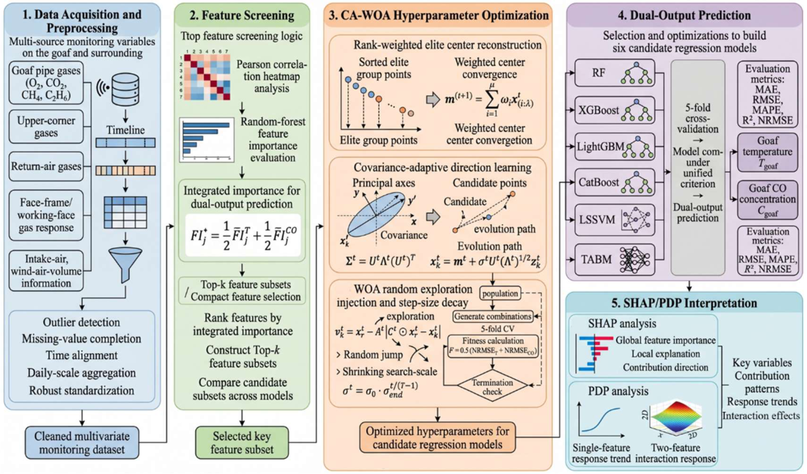
Figure 2.
Flowchart of the CA-WOA algorithm.
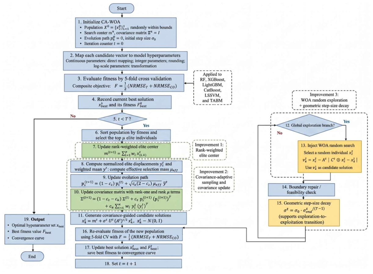
Figure 3.
Distribution of monitoring variables and prediction targets. (a) Distribution of robust-standardized input monitoring variables; (b) goaf temperature distribution; (c) goaf CO concentration distribution; (d) time-series variation of prediction targets.
Figure 3.
Distribution of monitoring variables and prediction targets. (a) Distribution of robust-standardized input monitoring variables; (b) goaf temperature distribution; (c) goaf CO concentration distribution; (d) time-series variation of prediction targets.
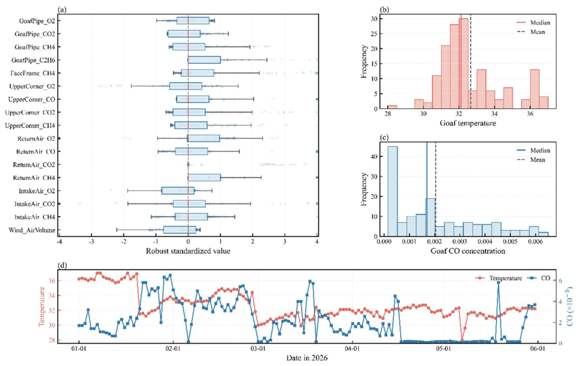
Figure 4.
Average fitness convergence curves of CA-WOA and competing algorithms on the CEC2022 test functions.
Figure 4.
Average fitness convergence curves of CA-WOA and competing algorithms on the CEC2022 test functions.
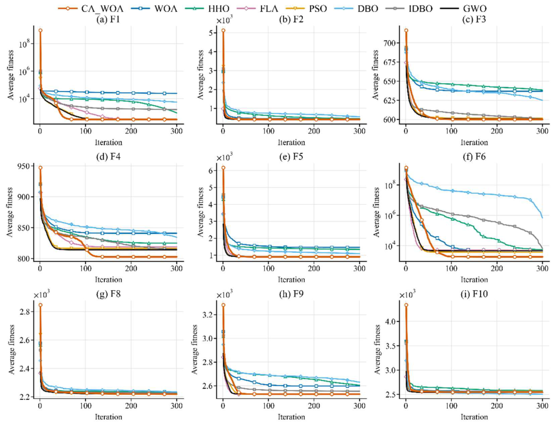
Figure 5.
Final fitness distributions of CA-WOA and competing algorithms on the CEC2022 test functions.
Figure 5.
Final fitness distributions of CA-WOA and competing algorithms on the CEC2022 test functions.
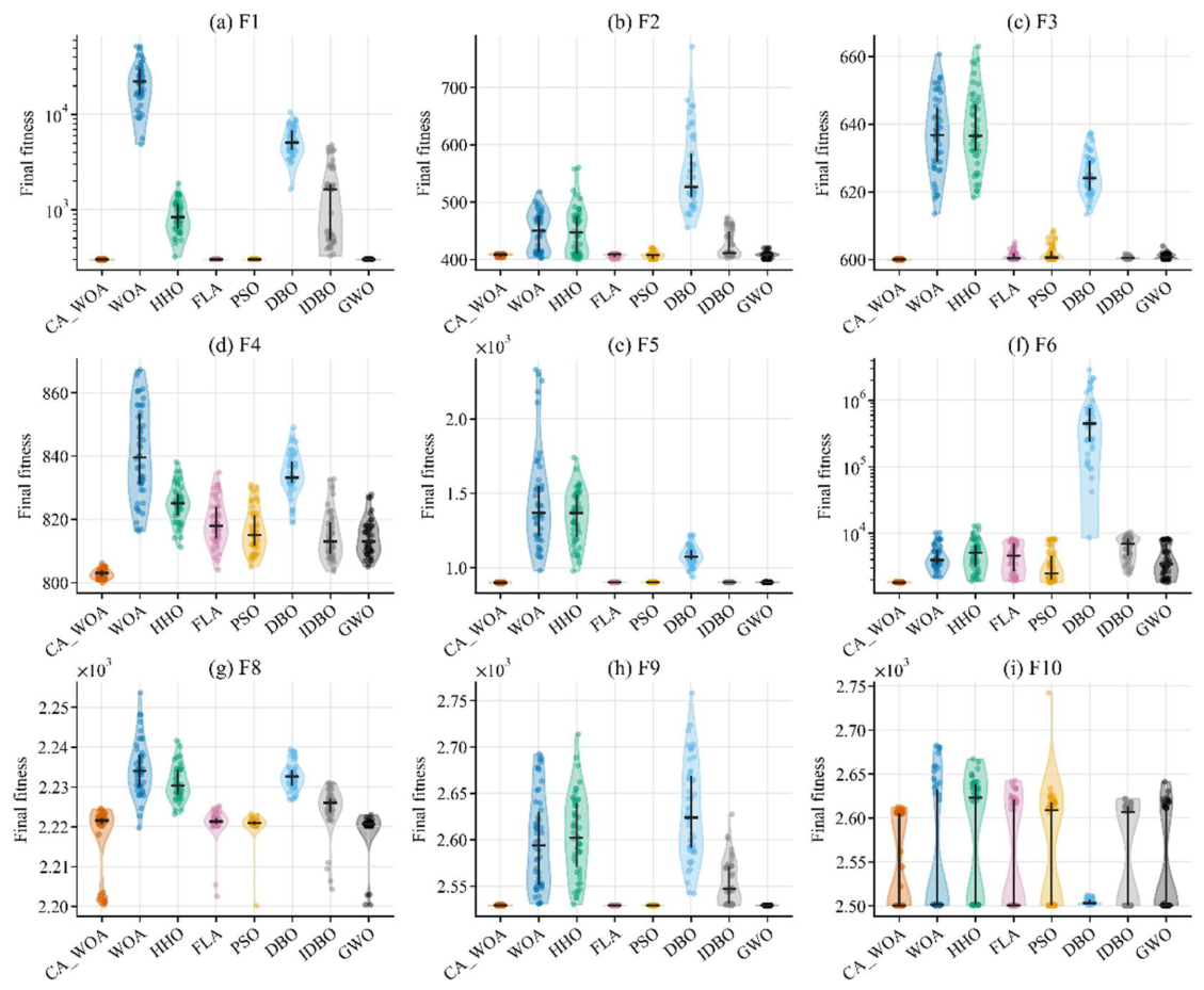
Figure 6.
Correlation heatmap of main features and prediction targets.
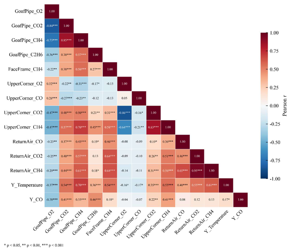
Figure 7.
Random forest feature-importance ranking of main features.
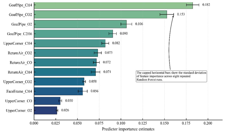
Figure 8.
Prediction performance of different top-
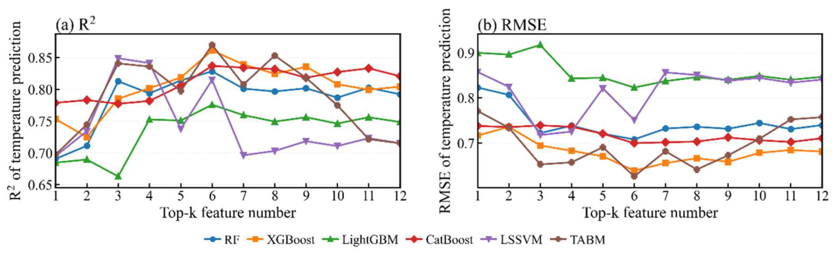
Figure 9.
Prediction performance of different top-
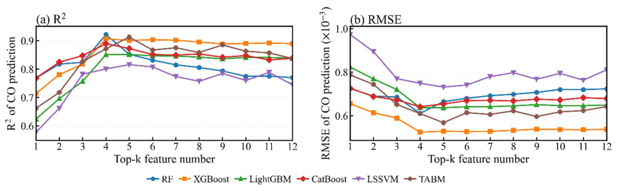
Figure 10.
Fitness convergence curves of the six CA-WOA-optimized models.
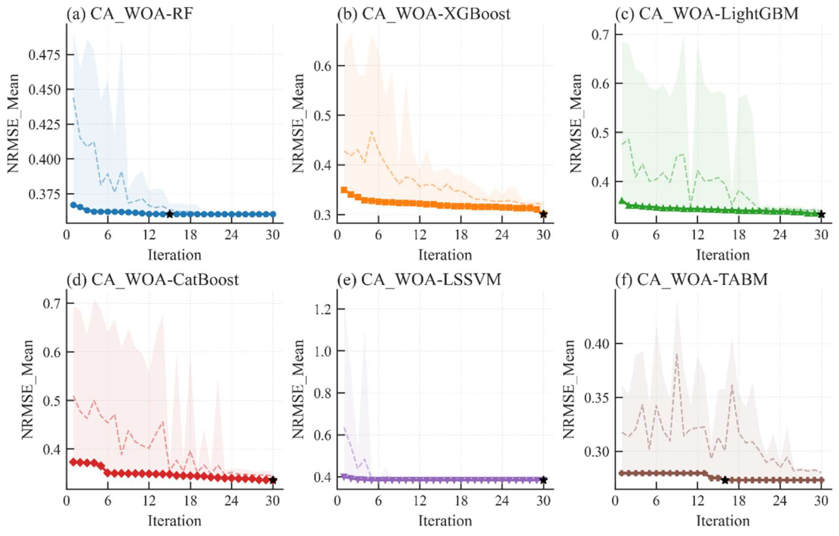
Figure 11.
Out-of-fold prediction comparison of goaf temperature and CO concentration under five-fold cross-validation.
Figure 11.
Out-of-fold prediction comparison of goaf temperature and CO concentration under five-fold cross-validation.
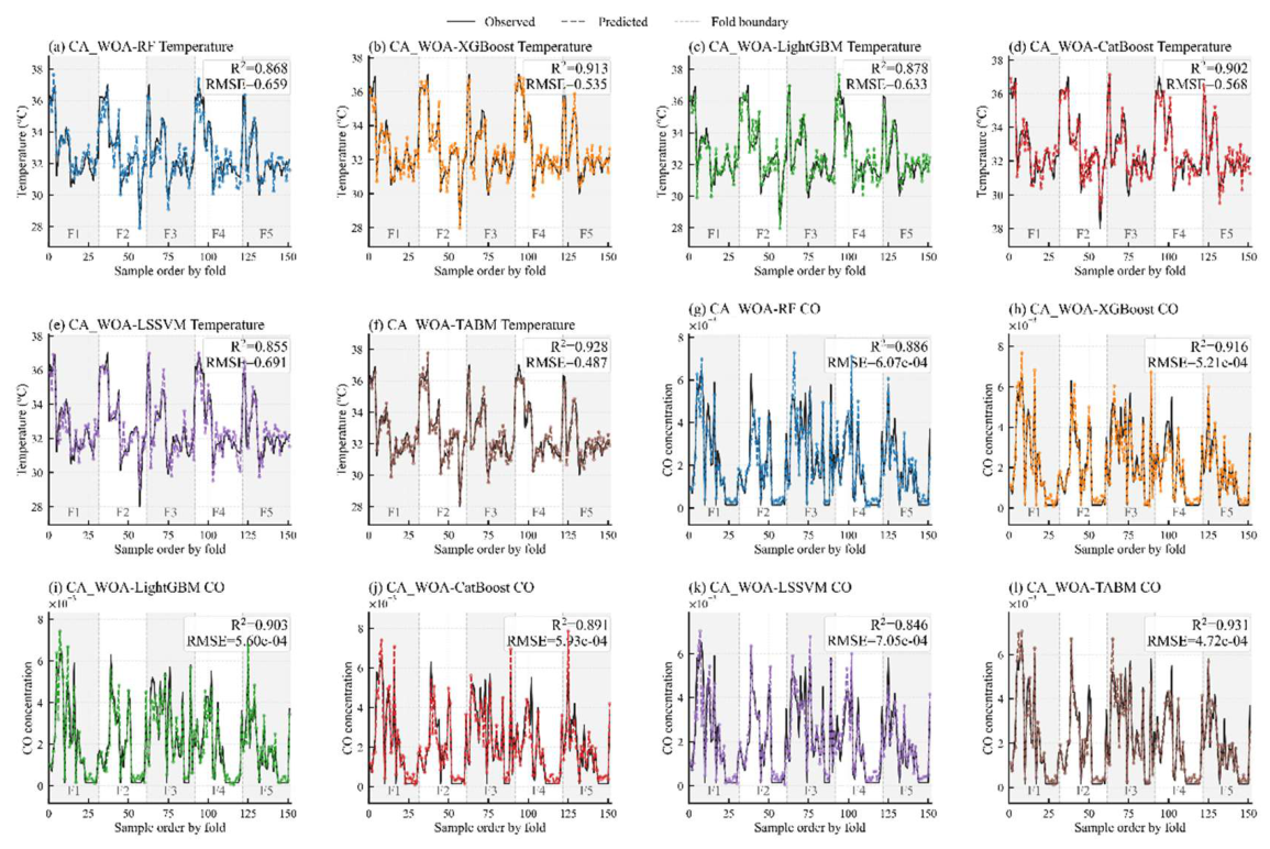
Figure 12.
Radar charts comparing baseline and CA-WOA-optimized models.
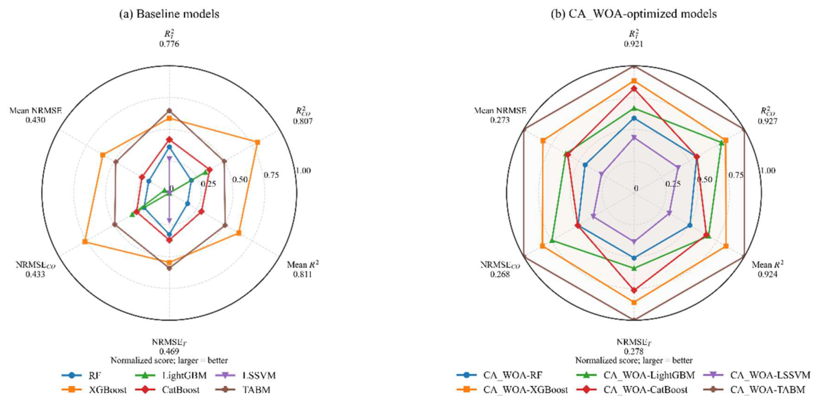
Figure 13.
Two-dimensional fitness response maps for key hyperparameters.
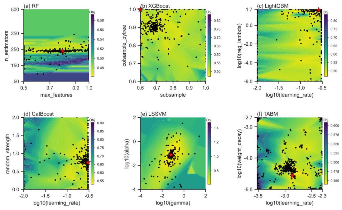
Figure 14.
SHAP/PDP interpretation of CA-WOA-XGBoost for goaf temperature prediction. (a) Mean absolute SHAP feature importance; (b) SHAP value distribution; (c) main and interaction SHAP effects; (d) SHAP interaction network; (e) SHAP heatmap across representative samples; (f) local SHAP explanation for a representative sample; (g) two-factor PDP response map of GP_CH4 and GP_CO2; (h) two-factor PDP response map of RA_CO2 and GP_CH4; (i) two-factor PDP response map of GP_C2H6 and GP_CO2; (j) two-factor PDP response map of GP_O2 and GP_CH4; (k) two-factor PDP response map of UC_CH4 and GP_CH4; (l) two-factor PDP response map of GP_CO2 and GP_CH4.
Figure 14.
SHAP/PDP interpretation of CA-WOA-XGBoost for goaf temperature prediction. (a) Mean absolute SHAP feature importance; (b) SHAP value distribution; (c) main and interaction SHAP effects; (d) SHAP interaction network; (e) SHAP heatmap across representative samples; (f) local SHAP explanation for a representative sample; (g) two-factor PDP response map of GP_CH4 and GP_CO2; (h) two-factor PDP response map of RA_CO2 and GP_CH4; (i) two-factor PDP response map of GP_C2H6 and GP_CO2; (j) two-factor PDP response map of GP_O2 and GP_CH4; (k) two-factor PDP response map of UC_CH4 and GP_CH4; (l) two-factor PDP response map of GP_CO2 and GP_CH4.
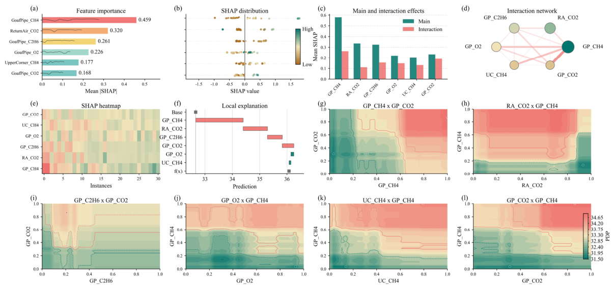
Figure 15.
SHAP/PDP interpretation of CA-WOA-XGBoost for goaf CO concentration prediction. (a) Mean absolute SHAP feature importance; (b) SHAP value distribution; (c) main and interaction SHAP effects; (d) SHAP interaction network; (e) SHAP heatmap across representative samples; (f) local SHAP explanation for a representative sample; (g) two-factor PDP response map of GP_CO2 and GP_O2; (h) two-factor PDP response map of GP_CH4 and GP_O2; (i) two-factor PDP response map of GP_C2H6 and GP_CH4; (j) two-factor PDP response map of GP_O2 and GP_CH4; (k) two-factor PDP response map of UC_CH4 and GP_CO2; (l) two-factor PDP response map of RA_CO2 and GP_CH4.
Figure 15.
SHAP/PDP interpretation of CA-WOA-XGBoost for goaf CO concentration prediction. (a) Mean absolute SHAP feature importance; (b) SHAP value distribution; (c) main and interaction SHAP effects; (d) SHAP interaction network; (e) SHAP heatmap across representative samples; (f) local SHAP explanation for a representative sample; (g) two-factor PDP response map of GP_CO2 and GP_O2; (h) two-factor PDP response map of GP_CH4 and GP_O2; (i) two-factor PDP response map of GP_C2H6 and GP_CH4; (j) two-factor PDP response map of GP_O2 and GP_CH4; (k) two-factor PDP response map of UC_CH4 and GP_CO2; (l) two-factor PDP response map of RA_CO2 and GP_CH4.
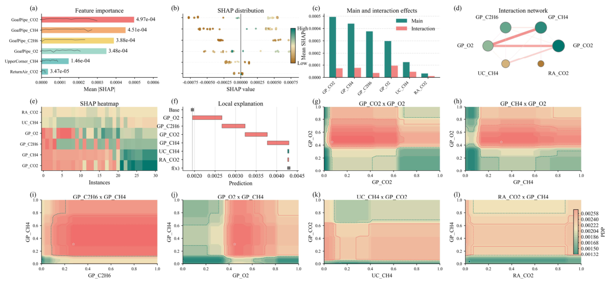

Table 1.
Overall ranking and win/tie/loss statistics of CA-WOA and competing algorithms on nine CEC2022 functions.
Table 1.
Overall ranking and win/tie/loss statistics of CA-WOA and competing algorithms on nine CEC2022 functions.
| Algorithm | Friedman mean rank | Overall rank | Top-3 count | W/T/L vs. CA-WOA |
|---|---|---|---|---|
| CA-WOA | 1.39 | 1 | 9 | — |
| FLA | 3.06 | 2 | 5 | 1/1/7 |
| IDBO | 3.5 | 3 | 6 | 0/1/8 |
| PSO | 3.94 | 4 | 3 | 0/1/8 |
| GWO | 4.56 | 5 | 3 | 0/0/9 |
| DBO | 6.22 | 6 | 1 | 1/0/8 |
| WOA | 6.61 | 7 | 1 | 0/0/9 |
| HHO | 6.72 | 8 | 0 | 0/0/9 |
Table 2.
Summary statistics of eight algorithms on nine representative CEC2022 functions.
| Function | CA-WOA | WOA | HHO | FLA | PSO | DBO | GWO | IDBO |
|---|---|---|---|---|---|---|---|---|
| F1 |
3.00×10² ± 1.99×10⁻¹⁴ |
2.60×10⁴ ± 1.50×10⁴ |
9.15×10² ± 3.47×10² |
3.00×10² ± 1.17×10⁻² |
3.00×10² ± 8.02×10⁻⁹ |
5.53×10³ ± 1.85×10³ |
1.73×10³ ± 1.67×10³ |
3.00×10² ± 2.55×10⁻⁹ |
| F2 | 4.07×10² ± 2.32×100 |
4.74×10² ± 8.64×101 |
4.52×10² ± 4.68×101 |
4.06×10² ± 3.00×100 |
4.12×10² ± 1.69×101 |
5.75×10² ± 1.04×10² |
4.26×10² ± 2.30×101 |
4.13×10² ± 1.87×101 |
| F3 |
6.00×10² ± 2.10×10⁻⁶ |
6.37×10² ± 1.12×101 |
6.38×10² ± 1.11×101 |
6.02×10² ± 3.04×100 |
6.03×10² ± 4.12×100 |
6.25×10² ± 5.89×100 |
6.01×10² ± 1.14×100 |
6.02×10² ± 2.59×100 |
| F4 |
8.03×10² ± 1.55×100 |
8.41×10² ± 1.47×101 |
8.25×10² ± 6.35×100 |
8.19×10² ± 7.01×100 |
8.18×10² ± 8.82×100 |
8.35×10² ± 7.46×100 |
8.15×10² ± 8.11×100 |
8.16×10² ± 9.67×100 |
| F5 |
9.00×10² ± 0.00×100 |
1.59×10³ ± 5.10×10² |
1.34×10³ ± 1.75×10² |
9.03×10² ± 7.46×100 |
9.09×10² ± 3.57×101 |
1.09×10³ ± 7.16×101 |
9.07×10² ± 1.54×101 |
9.06×10² ± 2.62×101 |
| F6 |
1.81×10³ ± 9.30×100 |
5.58×10³ ± 5.66×10³ |
5.84×10³ ± 4.20×10³ |
4.83×10³ ± 2.17×10³ |
3.66×10³ ± 2.23×10³ |
1.93×10⁶ ± 4.77×10⁶ |
6.53×10³ ± 2.19×10³ |
4.50×10³ ± 2.37×10³ |
| F8 | 2.22×10³ ± 7.61×100 |
2.24×10³ ± 1.12×101 |
2.24×10³ ± 1.90×101 |
2.22×10³ ± 4.62×100 |
2.23×10³ ± 2.85×101 |
2.23×10³ ± 6.85×100 |
2.23×10³ ± 1.81×101 |
2.24×10³ ± 4.16×101 |
| F9 |
2.53×10³ ± 5.86×10⁻¹¹ |
2.60×10³ ± 5.01×101 |
2.60×10³ ± 4.35×101 |
2.53×10³ ± 2.08×101 |
2.54×10³ ± 2.24×101 |
2.63×10³ ± 5.21×101 |
2.56×10³ ± 2.66×101 |
2.53×10³ ± 2.09×101 |
| F10 | 2.54×10³ ± 5.13×101 |
2.55×10³ ± 7.16×101 |
2.58×10³ ± 6.84×101 |
2.57×10³ ± 1.21×10² |
2.57×10³ ± 7.77×101 |
2.51×10³ ± 2.57×101 |
2.57×10³ ± 1.24×10² |
2.55×10³ ± 8.05×101 |
Table 3.
Baseline hyperparameter settings of candidate regression models.
| Model | Hyperparameter | Baseline value | Model | Hyperparameter | Baseline value |
|---|---|---|---|---|---|
| RF | n_estimators | 220 | RF | max_depth | 4 |
| RF | min_samples_leaf | 5 | RF | max_features | 0.7 |
| RF | n_jobs | 1 | |||
| XGBoost | n_estimators | 80 | XGBoost | max_depth | 2 |
| XGBoost | learning_rate | 0.04 | XGBoost | subsample | 0.8 |
| XGBoost | colsample_bytree | 0.8 | XGBoost | min_child_weight | 4 |
| XGBoost | reg_lambda | 8 | XGBoost | n_jobs | 1 |
| LightGBM | n_estimators | 90 | LightGBM | max_depth | 2 |
| LightGBM | learning_rate | 0.04 | LightGBM | subsample | 0.8 |
| LightGBM | colsample_bytree | 0.8 | LightGBM | min_child_samples | 12 |
| LightGBM | reg_lambda | 8 | LightGBM | n_jobs | 1 |
| CatBoost | iterations | 90 | CatBoost | depth | 2 |
| CatBoost | learning_rate | 0.04 | CatBoost | l2_leaf_reg | 20 |
| CatBoost | random_strength | 2 | CatBoost | thread_count | 1 |
| LSSVM | alpha | 10⁻³ | LSSVM | gamma | 0.005 |
| TABM | max_epochs | 300 | TABM | patience | 30 |
| TABM | lr | 1×10⁻³ | TABM | weight_decay | 3×10⁻⁴ |
| TABM | batch_size | 512 | TABM | d_block | 128 |
| TABM | n_blocks | 3 | TABM | k | 16 |
| TABM | dropout | 0.1 | TABM | val_fraction | 0.15 |
Table 4.
Hyperparameter search spaces and selected optimal values.
| Model | Hyperparameter | Search range | value | Model | Hyperparameter | Search range | value |
|---|---|---|---|---|---|---|---|
| RF | n_estimators | 50–500 | 239 | RF | max_depth | 2–20 | 17 |
| RF | min_samples_leaf | 1–8 | 1 | RF | max_features | 0.5–1.0 | 0.797948795 |
| XGBoost | n_estimators | 50–500 | 166 | XGBoost | max_depth | 2–10 | 6 |
| XGBoost | learning_rate | 0.01–0.30 | 0.3 | XGBoost | subsample | 0.6–1.0 | 0.6 |
| XGBoost | colsample_bytree | 0.6–1.0 | 1 | XGBoost | min_child_weight | 1–10 | 1 |
| XGBoost | reg_lambda | 10⁻⁶–50 | 50 | ||||
| LightGBM | n_estimators | 50–500 | 113 | LightGBM | max_depth | 2–12 | 6 |
| LightGBM | learning_rate | 0.01–0.30 | 0.26171755 | LightGBM | subsample | 0.6–1.0 | 0.755818689 |
| LightGBM | colsample_bytree | 0.6–1.0 | 0.827405489 | LightGBM | min_child_samples | 5–30 | 5 |
| LightGBM | reg_lambda | 10⁻⁶–50 | 42.39844725 | LightGBM | |||
| CatBoost | iterations | 50–500 | 335 | CatBoost | depth | 2–10 | 8 |
| CatBoost | learning_rate | 0.01–0.30 | 0.297133605 | CatBoost | l2_leaf_reg | 0.001–50 | 27.4900443 |
| CatBoost | random_strength | 0–2 | 0.746715595 | CatBoost | |||
| LSSVM | alpha | 10⁻⁴–100 | 0.077669431 | LSSVM | gamma | 10⁻⁴–100 | 0.06395764 |
| TABM | max_epochs | 180–420 | 315 | TABM | |||
| TABM | lr (learning_rate) | 3×10⁻⁴–0.005 | 0.001376567 | TABM | weight_decay | 10⁻⁵–0.002 | 2.7×10⁻⁵ |
| TABM | batch_size | 64–512 | 489 | TABM | d_block | 64–256 | 96 |
| TABM | n_blocks | 2–4 | 4 | TABM | k | 8–24 | 16 |
| TABM | dropout | 0–0.25 | 0.25 | TABM |
Table 5.
Five-fold average performance of the six CA-WOA-optimized base models.
| Model | R²_T | R²_CO | Mean R² | NRMSE_T | NRMSE_CO | F |
|---|---|---|---|---|---|---|
| CA-WOA-RF | 0.861±0.023 | 0.876±0.038 | 0.868±0.015 | 0.372±0.031 | 0.349±0.056 | 0.360±0.022 |
| CA-WOA-XGBoost | 0.904±0.037 | 0.907±0.052 | 0.905±0.021 | 0.305±0.064 | 0.296±0.083 | 0.300±0.033 |
| CA-WOA-LightGBM | 0.872±0.025 | 0.903±0.024 | 0.887±0.012 | 0.356±0.034 | 0.310±0.039 | 0.333±0.018 |
| CA-WOA-CatBoost | 0.895±0.023 | 0.876±0.039 | 0.885±0.023 | 0.323±0.036 | 0.349±0.057 | 0.336±0.034 |
| CA-WOA-LSSVM | 0.839±0.056 | 0.855±0.069 | 0.847±0.054 | 0.396±0.074 | 0.372±0.090 | 0.384±0.071 |
| CA-WOA-TABM | 0.921±0.028 | 0.927±0.017 | 0.924±0.020 | 0.278±0.050 | 0.268±0.033 | 0.273±0.036 |
Table 6.
Comparison of comprehensive model performance before and after CA-WOA optimization.
| Model | Before Mean R² | After Mean R² | Improvement | Before F | After F | Reduction |
|---|---|---|---|---|---|---|
| RF | 0.83 | 0.868 | 0.039 | 0.401 | 0.36 | 10.10% |
| XGBoost | 0.882 | 0.905 | 0.023 | 0.336 | 0.3 | 10.50% |
| LightGBM | 0.811 | 0.887 | 0.076 | 0.423 | 0.333 | 21.30% |
| CatBoost | 0.844 | 0.885 | 0.041 | 0.391 | 0.336 | 14.10% |
| LSSVM | 0.811 | 0.847 | 0.036 | 0.43 | 0.384 | 10.80% |
| TABM | 0.868 | 0.924 | 0.056 | 0.354 | 0.273 | 22.80% |
Table 7.
Out-of-fold prediction performance under five-fold cross-validation.
| Model | R²_T | RMSE_T | R²_CO | RMSE_CO |
|---|---|---|---|---|
| CA-WOA-RF | 0.868 | 0.659 | 0.886 | 6.07×10⁻⁴ |
| CA-WOA-XGBoost | 0.913 | 0.535 | 0.916 | 5.21×10⁻⁴ |
| CA-WOA-LightGBM | 0.878 | 0.633 | 0.903 | 5.60×10⁻⁴ |
| CA-WOA-CatBoost | 0.902 | 0.568 | 0.891 | 5.93×10⁻⁴ |
| CA-WOA-LSSVM | 0.855 | 0.691 | 0.846 | 7.05×10⁻⁴ |
| CA-WOA-TABM | 0.928 | 0.487 | 0.931 | 4.72×10⁻⁴ |
Disclaimer/Publisher’s Note: The statements, opinions and data contained in all publications are solely those of the individual author(s) and contributor(s) and not of MDPI and/or the editor(s). MDPI and/or the editor(s) disclaim responsibility for any injury to people or property resulting from any ideas, methods, instructions or products referred to in the content. |
© 2026 by the authors. Licensee MDPI, Basel, Switzerland. This article is an open access article distributed under the terms and conditions of the Creative Commons Attribution (CC BY) license (http://creativecommons.org/licenses/by/4.0/).
Copyright: This open access article is published under a Creative Commons CC BY 4.0 license, which permit the free download, distribution, and reuse, provided that the author and preprint are cited in any reuse.


