
Submitted:
23 June 2026
Posted:
25 June 2026
You are already at the latest version
Abstract
Vehicle-to-grid (V2G) integration in commercial building microgrids (CBMGs) offers a promising path for grid support, economic arbitrage, and resilience enhancement. However, practical implementation is hindered by the optimization-execution gap, where high-level aggregated commands fail to match low-level physical charger capacities and individual battery boundaries, and by the lack of socio-technical coupling under extreme weather events where vehicle owner range anxiety dominates. To address these challenges, a closed-loop multi-timescale energy management system for V2G-enabled CBMGs under exogenous meteorological conditions is proposed. The framework features an integrated four-layer cyber-physical control architecture connecting macroscopic day-ahead scheduling, receding-horizon model predictive control (MPC), discrete real-time parking slot allocation with hardware safety boundary constraints, and equipment-level power flow execution. To handle extreme events, an exogenous meteorological stress index is formulate to quantify ambient structural hazards and temperature deviations, mapping them to owner range anxiety and loss-aversion behaviors using prospect theory. Rather than relying on heuristic rule-switching, the optimizer executes a smooth and continuous transition from normal economic peak-shaving to active pre-disaster energy reservation and load demand survival. The cyber-physical system is validated using high-fidelity co-simulations under typical summer and winter blizzard scenarios. The results demonstrate that the proposed hierarchical architecture successfully eliminates optimization-execution mismatches and guarantees zero load shedding. Furthermore, sensitivity analyses establish the optimal system configuration with the critical defense tolerance of 0.6 and the baseline anxiety ratio of 4, which successfully resolves the trade-off between premature defensive actions and insufficient energy reserves while considering the human behavioral uncertainty.
Keywords:
microgrid
; vehicle-to-grid
; optimization
1. Introduction
At the grid edge, modern power distribution infrastructures are increasingly exposed to a rising frequency and intensity of climate-driven, high-impact, low-probability (HILP) meteorological stressors [1,2]. This exogenous environmental vulnerability is particularly pronounced within commercial building microgrids (CBMGs), where localized cyber-physical subsystems are tightly coupled [3,4,5].
Specifically, intense meteorological hazards such as blizzards and cold snaps generate a severe "operational scissor gap" at the grid edge: they simultaneously trigger an exponential spike in weather-sensitive HVAC loads due to aggressive thermal comfort demands, while inducing abrupt solar irradiance attenuation and snow-soiling effects that collapse distributed photovoltaic (PV) generation [6]. Concurrently, the destructive wind gusts inherent to such winter storms significantly increase local infrastructure tripping probabilities. Consequently, this multi-domain extreme coincidence severely compresses the microgrid’s real-time operational feasible domain, rendering conventional price-based static dispatch schedules obsolete and posing an immediate threat to grid-edge load preservation and infrastructure resilience [7,8].
To mitigate these volatile, high-capacity power mismatches and artificially expand the microgrid’s compressed operational envelope, leveraging flexible demand-side resources has emerged as a necessary solution. Within commercial complexes, a large-scale fleet of hundreds of electric vehicles (EVs) integrated via vehicle-to-grid (V2G) technology represents a flexible distributed energy resource [9,10].
By systematically coordinating discrete EV session data—encompassing stochastic arrival/departure timestamps, dwell durations, and individualized state-of-charge (SOC) boundary constraints—this heterogeneous vehicular cluster can be macroscopically aggregated into a high-capacity virtual energy storage system (VESS) [11]. Under nominal, unperturbed meteorological conditions, this VESS offers high operational flexibility. Conventional price-based scheduling frameworks can seamlessly exploit this aggregated capacity to execute trans-temporal economic arbitrage; by charging during low-tariff valley periods and executing V2G peak-shaving during maximum-demand hours, the centralized controller can minimize net daily electricity expenditure while effectively stabilizing the microgrid’s load profile [12,13].
Extensive literature has investigated the grid-edge integration of EVs, with existing state-of-the-art frameworks demonstrating successful performance in standard demand-side management and steady-state economic dispatch [10,14,15]. However, deploying traditional centralized mathematical optimization frameworks—such as individual-tracking mixed-integer linear programming (MILP) or model predictive control (MPC)—to govern such VESS networks becomes fundamentally intractable under catastrophic environmental emergencies [15,16,17,18,19,20]. First, the framework suffers from a severe curse of dimensionality; because each individual vehicle session introduces integer charging/discharging indicators and coupled boundary profiles over a multi-period receding horizon, the centralized decision matrix for hundreds of EVs leads to a high-dimensional, non-convex mixed-integer optimization problem that is computationally intractable [21]. The resulting exponential optimization latency will overshoot the sub-minute execution window required at the grid edge. Second, existing literature predominantly operates on hourly or 15-minute dispatch intervals [22]. During winter blizzards, the system is exposed to high-frequency solar irradiance fluctuations and dynamic wind gusts. Coarse-grained optimizations cannot capture these intra-interval variations, causing cumulative tracking divergence and localized stochastic violations. In a practical cyber-physical microgrid, such uncontrolled real-time power shortages trigger post-event forced hardware tripping of local protective relays, which leads to severe cascading load shedding.
Beyond these computational challenges, contemporary microgrid resilience studies exhibit limitations due to the decoupling of system scheduling from human mobility. The vast majority of system-level energy management algorithms treat the EV fleet as passive, stationary battery storage units with static power constraints [23,24,25,26]. Under intense meteorological stress, when the centralized solver is forced to aggressively extract energy via V2G peak-shaving to defend building loads, the individual, human-centric session boundaries become entirely opaque to the cyber layer. Lacking real-time visibility into specific arrival-departure timestamps or user-defined expected departure SOC, conventional heuristic or economic-driven rules frequently over-deplete vehicular energy resources in the real-time loop, forcefully breaching electrochemical safety margins. This aggressive depletion not only induces severe, rainflow-counted battery capacity fade and structural degradation, but also inflates user departure anxiety and degrades system trust. Consequently, ignoring the deep coupling between physical grid resilience and human mobility constraints renders existing mathematical schedules unviable in realistic commercial environments with human-in-the-loop.
To address these limitations, this paper proposes a socio-technical, closed-loop, multi-timescale energy management system for V2G-enabled CBMGs driven by exogenous meteorological stress. By bridging the gap between high-level economic optimization and low-level physical execution, this cyber-physical framework ensures that scheduling commands are strictly physically feasible while exhibiting robust resilience under extreme weather events. The key contributions of this paper are summarized as follows:
- 1.
- We develop an exogenous, meteorologically-driven operational stress index, denoted as , that mathematically links extreme weather progression with the socio-technical utility of EV owners. Rooted in prospect theory [27,28], the formulation quantifies owner anxiety and panic-driven charging behavior as dynamic utility penalties, establishing a robust socio-technical scheduling paradigm under extreme HILP events.
- 2.
- Unlike conventional resilient scheduling that relies on heuristic, discrete state-switching triggers, our mathematical MILP and receding-horizon MPC formulations execute an autonomous, smooth algorithmic transition. Under weather stress, as approaches unity, the optimization seamlessly shifts its operational trajectory from economic arbitrage to emergency survival, load-shedding prevention, and energy reservation.
- 3.
- We propose a closed-loop multi-timescale energy management system that connects macroscopic hourly day-ahead scheduling in Layer 1, mid-term 15-minute receding-horizon MPC in Layer 2, 10-second discrete charging port and power allocation with hardware safety boundary constraints in Layer 3, and real-time microgrid power flow execution in Layer 4. This framework resolves the severe optimization-execution mismatches under strict parking spot capacity limits and physical battery boundaries.
The remainder of this paper is organized as follows. Section II establishes the physics-driven characterization of exogenous meteorological stressors and microgrid resilience formulation. Section III formalizes the closed-loop multi-timescale energy management system with a macroscopic EV fleet aggregation mode. Section IV details the modeling foundations and scenario generation framework for establishing a rigorous and reproducible validation environment for the proposed hierarchical energy management system. Performance benchmarking across seasonal baseline operations, extreme weather resilient scenarios, and dual-parametric sensitivity analysis is scrutinized in Section V. Finally, Section VI provides the conclusion.
2. Meteorological Stress and Microgrid Resilience Formulation
To establish a mathematically rigorous and credible foundation for microgrid resilience, this paper establishes an exogenous meteorological stress modeling that maps raw weather conditions to socio-technical resilient behaviors. Unlike traditional resilience assessment frameworks that rely on retrospective, endogenously-coupled damage reports, the formulated approach strictly isolates the exogenous meteorological hazard from internal microgrid operational states. This design aligns with feedforward control theory [29], mathematically eliminating the algebraic circular dependency loop wherein the environmental stress assessment endogenously depends on the system’s own dispatch actions. Crucially, because the stress trajectory is purely exogenous, mathematical consistency is guaranteed across multi-temporal operational horizons, thereby safeguarding the numeric stability of both global scheduling and short-term receding-horizon regulation loops.
2.1. Exogenous Meteorological Stress Formulation
Three exogenous, physically decoupled weather stressors are defined representing the multi-dimensional physical threats of extreme events:
2.1.1. Wind Speed Factor
Wind speed factor is defined as Eq. (1) reflecting the physical destruction probability of wind velocities on distribution power lines, poles, and PV solar tracking brackets [30]:
where is the raw wind velocity; defines the baseline threshold below which ambient wind speeds impose negligible physical stress or tripping risks on local grid-edge lines; and represents the critical design-scaling wind velocity parameter at or beyond which the normalized wind speed factor saturates to unity.
2.1.2. Temperature Deviation Factor
To evaluate the localized thermodynamic stress imposed on the building energy system under severe thermal anomalies, the normalized temperature deviation factor, denoted as , is formulated. This metric is rigorously aligned with the occupant thermal comfort boundaries specified in the ANSI/ASHRAE Standard 55 [31], analytically characterizing the non-linear temperature-vulnerability profile of typical commercial structures:
where represents the dry-bulb ambient temperature; and define the upper and lower boundary thresholds of the standard indoor thermal comfort envelope, respectively; denotes the deterministic reference normalization margin.
2.1.3. Solar Irradiance Loss Factor
Solar irradiance loss factor represents the absolute physical solar shielding caused by cloud cover, dust storms, or snow accumulation:
where is the actual global horizontal solar irradiance, is the theoretical clear-sky solar irradiance calculated based on the geographical coordinates of the building, and is a night-time filtering threshold to avoid singularities.
By assigning prior operational weights to these decoupled stressors, we construct the composite exogenous meteorological hazard index representing the absolute exogenous environmental threat:
where , , and are weighting coefficients satisfying , calibrated based on the microgrid’s regional climate characteristics and operational sensitivities.
Finally, to map the environmental threat to a normalized cyber-metric, we couple with the system’s physical design tolerance using a continuous, differentiable logistic sigmoidal activation function to evaluate the integrated operational stress index [30,32] :
where is the critical stress inflection threshold between 0 and 1, mathematically defining the symmetric midpoint of the sigmoidal locus. Physically, captures the structural turning point of perceived meteorological stress within the cyber layer; when reaches , the exponent nullifies, yielding set to 0.5, representing the threshold below which the microgrid can absorb external hazards without requiring load shedding, and is a transition steepness parameter governing the steepness of the structural transition from economic mode to emergency survival mode.
2.2. Socio-Technical Resilience Formulation
According to prospect theory [27,28], human utility valuation fundamentally shifts under high-risk scenarios, transforming nominal economic trading into a survival-oriented loss domain where EV owners systematically curtail V2G capacity to safeguard personal mobility. Simultaneously, extreme meteorological stress necessitates the adaptive defense of physical assets, requiring the prioritization of building load preservation over grid arbitrage and the strict enforcement of survival energy reserves to prevent premature battery energy storage system (BESS) depletion. To continuously integrate these multi-domain resilience requirements—encompassing mobility behavioral dynamics, load-shedding penalties, and BESS capacity margins—into the convex optimization framework without introducing computationally expensive binary integer variables, three stress-dependent penalty functions are formulated as Eqs. (6)–(10).
To capture the coupled socio-technical interaction between human loss-aversion and grid-edge flexibility, a mobility anxiety penalty coefficient is formulated:
where is the dimensionless baseline anxiety ratio, standardizing the psychological utility cost relative to the on-peak electricity purchasing price , and is the exponential scaling parameter. Aligned with empirical discrete choice frameworks under risk and emergency evacuation behaviors [33], this formulation mathematically characterizes the non-linear loss-aversion behavior of EV owners. As the meteorological stress index increases, the penalty coefficient escalates exponentially, heavily penalizing the V2G dispatch power trajectory in the optimization objective to preemptively safeguard individual mobility capacity.
To prioritize building load preservation over grid arbitrage under extreme weather stress, a dynamic load shedding penalty function is formulated as:
where denotes the baseline load-shedding penalty coefficient under nominal conditions, and represents the exponential scaling parameter governing the penalty steepening rate as meteorological stress intensifies.
To prevent BESS depletion prior to potential grid disruptions, a dynamic survival energy reserve is enforced:
This dynamic reserve is integrated into the optimization horizon via soft capacity constraints:
where is the energy stored in the BESS; denotes the minimum allowable capacity bound; represents the critical survival capacity threshold; is the non-negative reserve violation slack variable; and the corresponding penalty weight is adaptively scaled as:
where is the baseline penalty coefficient enforcing reserve defense during the pre-disaster phase, and is the scaling sensitivity factor. Physically, reducing under rising stress prioritizes load survival over reserve conservation. As approaches 1, the exponential escalation of the load-shedding penalty in Eq. (7) combined with the relaxation of establishes a hierarchical operational priority, allowing the optimization framework to violate the soft reserve constraint in Eq. (9) and release stored energy to prevent building load shedding.
By establishing this socio-technical resilient formulation, the stress index functions as a feedforward signal, seamlessly transitioning the control objective from economic arbitrage to emergency resilience enhancement.
3. Closed-Loop Multi-Timescale Energy Management System
3.1. Four-Layer Framework Overview
Based on the exogenous meteorological stress index and resilience formulations established in Section II, the control engine must systematically translate these high-level risk profiles into real-time physical power dispatch commands. To bridge the optimization-execution gap under rigid grid-edge and port capacity constraints, the proposed framework deploys a hierarchical, four-layer control architecture, as illustrated in Figure 1. These structural layers are dynamically coupled via reciprocal trajectory-tracking feedback loops:
- 1.
- Layer 1 executes day-ahead economic scheduling at an hourly resolution, generating global economic and resilient baseline trajectories driven by the exogenous meteorological forecasts.
- 2.
- Layer 2 performs intra-day receding-horizon optimization at a 15-minute resolution, serving as the coordination unit to mitigate forecasting uncertainties and stochastic load-generation fluctuations.
- 3.
- Layer 3 manages real-time EV dispatching at a 10-second sampling interval, dynamically mapping the upper-layer aggregated commands onto N physical charging spots while strictly respecting individual EV safety envelopes.
- 4.
- Layer 4 enforces instantaneous microgrid power control at the same 10-second scale, functioning as the continuous physical actuator to maintain DC bus voltage stability and real-time power balance.
To ensure computational tractability across Layers 1 and 2, a macroscopic aggregation model is formulated to reduce the dimensionality of the decentralized EV fleet.
3.2. Macroscopic EV Fleet Aggregation Model
To circumvent high-dimensional single-vehicle variables within the day-ahead and intra-day scheduling horizons, the spatially distributed EV fleet is mathematically aggregated into a macroscopic VESS model. This state-space reduction is restricted exclusively to the upper optimization layers to guarantee real-time computational tractability.
The aggregate energy stored within the EV fleet at time step t, denoted as , is expressed as:
where represents the time-varying set of active vehicles plugged into the charging ports during hour t, and is the nominal electrochemical capacity of EV i. The macro-scale state transition of the EV VESS, which continuously accounts for bidirectional power delivery and transport traffic flows, is established as:
where and represent the charging and discharging efficiencies, and are the fleet-level aggregated purchase and injection power commands, is the cumulative energy injected into the system boundary by arriving EVs:
signifies the cumulative energy leaving the boundary via departing EVs:
where and are the arrival SOC and the expected departure SOC of EV i, and denote the localized arriving and departing EV sub-sets at time step t, respectively.
3.3. Layer 1: Day-Ahead Optimization Layer
The day-ahead optimization layer aggregates all active EVs into a single VESS bounded by time-varying energy envelopes. The objective function minimizes the total operational cost, comprising utility grid trading costs, , battery degradation costs, , of the BESS and EVs, and load-shedding and resilience-reserve penalties, . The objective function adaptively balances economic arbitrage incentives and system resilience requirements using the exogenous stress index as an adaptive modulating signal:
where the utility grid trading cost is formulated as Eq. (16). The microgrid imports energy from the utility grid during off-peak intervals and exports surplus PV generation or V2G power during peak-tariff periods.
where and are the utility grid purchasing and feed-in electricity tariffs, respectively.
To guarantee convex tractability within the upper optimization layers, battery degradation costs for both the BESS and the macroscopically aggregated EVs are characterized via a linearized throughput-based penalty mechanism:
where and are the degradation cost coefficients for the BESS and EV batteries, respectively.
To avoid heuristic, rule-based binary switches that introduce non-convexities and high computational overhead, the upper optimization layers leverage the exogenous meteorological stress index to enforce a smooth, continuous functional transition across distinct operational priority domains:
where the dynamic penalty coefficients , , and are strictly defined by Eqs. (7)–(10), represents the PV curtailment penalty coefficient introduced to enhance renewable energy utilization.
To ensure that the mathematical economic dispatch commands do not violate continuous microgrid infrastructure limits, the optimization is strictly subject to the following multi-energy flow equations including utility grid interconnection power bounds, microgrid power balance constraint, BESS electrochemical state transition and constraints in Eqs. (19)–(25).
To ensure physical exclusivity of the utility power import and export under bidirectional tariffs, the following constraints are imposed:
where is the transformer physical limit and is the binary grid import status variable.
The active power balance equation at the microgrid bus is expressed as:
where and represent the predicted solar generation and building load demand profiles, respectively.
BESS electrochemical state transition and constraints are shown as following:
where and are BESS charging and discharging efficiencies, and is the binary BESS operational indicator preventing concurrent charging and discharging. The state transition is initialized with the real-time initial feedback state.
Under standard weather conditions, the penalties on EV anxiety and BESS hoarding is reduced to a base level, enabling the scheduler to optimize for economic arbitrage. As extreme weather events approach, the penalty scaling functions dynamically prioritize building load protection and compel the BESS to accumulate defensive energy reserves, smoothly shifting the system from economic mode to resilient emergency survival. The outputs of Layer 1 are the optimal trajectories for the BESS state of charge and the aggregated EV power profile where the latter is formulated as the difference between and .
3.4. Layer 2: Intra-Day Optimization Layer
To compensate for PV forecasting errors and stochastic real-time EV arrival/departure variations, Layer 2 runs online at a 15-minute resolution over a receding horizon H, and re-optimizes the economic cost within the horizon while strictly penalizing deviations from the day-ahead references to preserve long-term economic optimality:
where , , and represent the real-time utility grid trading, degradation, and stress penalty costs, respectively. The EV virtual battery states and BESS capacity over the receding prediction horizon are subject to the same physical structures as in (11)–(14) and (22)–(25) . is the tracking error of the aggregated EV power, enforced via the soft constraints:
similarly, represents the terminal BESS energy tracking error at the end of the MPC horizon , forcing the BESS to align with the long-term economic reference :
Layer 2 outputs the optimal real-time aggregated EV power reference and the BESS power reference for physical execution.
3.5. Layer 3: Real-Time EV Energy Management Layer
The primary challenge in deploying mathematical scheduling to real-world cyber-physical microgrids is the operational mismatch between the macroscopic VESS abstraction used in the upper optimization layers and the discrete constraints of physical charging ports in the parking lot. Layer 3 and Layer 4 bridge this gap by executing high-frequency allocation and real-time physical power-voltage stabilization.
Layer 3 operates at a 10-second resolution, serving as the critical cyber-physical translation bridge that maps the macroscopically aggregated power reference into discrete EVs execution commands under strict infrastructural boundaries.
When the number of the daily EV arrivals exceeds the available physical charging infrastructure, mathematical optimization assuming infinite parallel charging ports becomes physically infeasible. To address this physical constraint, a deterministic state-machine queue is established based on the sequential time of arrival to manage the N fixed parking spots. EVs are admitted and plugged into charging ports strictly in chronological order. Once all N spots are occupied, newly arriving EVs are restricted from receiving power commands and maintained in a deferred standby status. This infrastructure-induced execution deviation forces the physical system to temporarily separate from upper-layer unconstrained predictive profiles. The resulting actual parking status is continuously fed back to the upper optimization layers at the subsequent time step, effectively closing the cyber-physical control loop.
Prior to distributing power to individual EVs, the macroscopically aggregated command generated by the upper optimization layers must be reconciled with real-time microgrid security envelopes. Specifically, the raw reference profile is dynamically projected onto the safety corridor bounded by the maximum allowable charging power cap, , and the maximum allowable discharging floor, , yielding a rectified tracking target:
To guarantee that V2G discharging operations do not leave EV owners stranded upon departure, Layer 3 constructs a dynamically sliding SOC limit for each active EV i. An EV is eligible to perform discharging only if its current energy state possesses sufficient temporal and hardware headroom to fully recover to the requested departure target under maximum continuous charging power before its scheduled departure time. The time-coupled recovery threshold is formalized as:
where is the maximum continuous EV charging power limit of the individual charging port, is the scheduled departure timestamp.
To protect EV batteries from excessive depth-of-discharge and ensure emergency mobility, the allowable discharging boundary is strictly locked by a dual-protection safety limit. The finalized lower SOC threshold, denoted as , is governed by the maximum operator between a rigid physical depletion limit and the time-coupled recovery constraint:
where denotes the absolute lower physical limit to prevent accelerated capacity fade, which is typically fixed at 20%. Based on this sliding limit value, the EV dispatch mechanism partitions the fleet into two mutually exclusive control streams: EVs whose instantaneous energy states have drifted to or below the finalized lower SOC threshold, satisfying , are immediately locked into a rigid grid-to-vehicle charging mode and allocated their maximum physically allowable intake power. When the upper-layer scheduling dictates a fleet-level collective discharging command, only EVs satisfying the strict dual-protection headroom constraint and possessing active bidirectional V2G authorization are permitted to discharge power back to the building microgrid.
Due to the uncoordinated power draw of must-charge EVs, the aggregated allocation may exceed the microgrid capacity limit. To protect local infrastructure, an urgency-based power truncation algorithm is executed at the end of the allocation step. The algorithm computes a continuous time-slack metric, denoted as , for all EVs currently undergoing charging:
where represents the minimum continuous duration required for EV i to fulfill its departure energy target under its maximal power charging conditions.
The metric quantifies the temporal safety margin of each EV. A larger value of signifies that the corresponding EV possesses an abundant time window to defer its charging activity to a later period. Consequently, the truncation algorithm sorts all charging EVs in descending order according to and sequentially curtails their charging power commands until the aggregated power allocation strictly converges to . This safety corridor bounding and sorting structure insulates the localized building microgrid from uncoordinated overloads while satisfying individual user mobility utility.
3.6. Layer 4: Real-Time Microgrid Power Control Layer
Layer 4 is embedded within the continuous-time physical execution stage, operating at a 10-second interval. Rather than relying on unconstrained mathematical optimization, Layer 4 governs the localized microgrid through a deterministic, cascaded priority dispatch structure. Crucially, Layer 4 functions as the bidirectional interface that coordinates the macroscopic cyber layer with individual EV micro-controllers by dynamically enforcing the absolute power flow hierarchy.
Prior to Layer 3 allocation, Layer 4 performs a high-frequency look-ahead screening of the local infrastructure margins to enforce the power balance priority chain. Under this scheme, the EV fleet is treated as an adjustable energy resource, ranked downstream of the building load but upstream of the stationary BESS and the utility grid. To dynamically restrict individual EV commands within safe limits, Layer 4 pre-calculates the maximum continuous power envelopes that the aggregated EVs are physically permitted to absorb or discharge.
The maximum allowable charging power cap allocated to the fleet, denoted as , is governed by the instantaneous net PV generation surplus combined with the maximum continuous discharging capability of the BESS and the physical import capacity of the utility grid transformer:
where is the real-time solar generation, represents the load demand of the commercial building, is the maximum continuous discharge threshold of the stationary battery, and is the continuous thermal limit for the utility grid power import.
Conversely, the maximum allowable discharging floor for V2G operations, denoted as , defines the absolute reverse power containment wall. This lower envelope is derived by matching the net local generation surplus with the maximum continuous charging capacity of the BESS and the maximum reverse power absorption limit of the utility grid interconnection:
where is the maximum charging power limit of the BESS, and represents the maximum allowable export power to the utility grid. By continuously feeding these two dynamic envelopes forward to Layer 3, Layer 4 guarantees that the aggregated EVs tracking reference strictly respects the localized multi-energy resource availability.
Once the discrete single-EV charging states are finalized by Layer 3, the actual aggregate power flow of the EVs, denoted as , is captured by physical sensors. To guarantee instantaneous power balancing, the real-time net power imbalance across the microgrid power bus is formalized as:
To maintain absolute microgrid power equilibrium and stabilize the bus voltage against high-frequency forecasting errors, a multi-stage cascaded correction loop is executed sequentially across the active energy resources. In the primary phase, the local controller coordinates with Layer 2 by extracting the MPC charging-discharging reference command, denoted as , and enforcing it onto the BESS. The residual power discrepancy after integrating the optimization reference is calculated as:
Based on the sign and magnitude of , the physical layer activates a hierarchical protection sequence with two scenarios, scenario A and scenario B, to systematically absorb real-time fluctuations.
In scenario A, is greater than 0, which means the residual discrepancy indicates a localized electricity shortage. The utility grid is primarily activated to deliver power up to its hardware capacity limit:
If the deficit cannot be fully covered by the utility grid due to the transformer power limit, the BESS is commanded to bypass its optimization trajectory and discharge its remaining available power to support the microgrid:
In extreme circumstances where the combined delivery capacity of the saturated transformer and the fully depleted BESS cannot stabilize the DC bus, the physical layer triggers emergency load shedding to prevent bus voltage collapse:
In scenario B, the is less than 0, which means the PV introduces an excess energy profile, the surplus is routed back to the utility grid for commercial transaction within the localized interconnection threshold:
If the reverse power flow hits the interconnection limit, the BESS overrides its upper-layer reference to absorb the remaining excess power using its charging capability limit:
If the BESS capacity is fully saturated and the utility grid reaches its limit, the physical execution layer activates inverters to perform real-time PV power curtailment:
Through this four-layer hierarchical control architecture, Layer 3 and Layer 4 successfully decouple upper-level macroscopic optimization trajectories from high-frequency physical imbalances, guaranteeing microgrid survivability under severe optimization-execution mismatches.
4. Modeling Foundations and Scenario Generation Framework
To establish a rigorous and reproducible validation environment for the proposed hierarchical energy management system, this section formalizes a data-driven offline scenario-generation framework in Figure 2. As illustrated in the unified data pipeline, the validation core couples multi-source empirical datasets—specifically, the National Household Travel Survey (NHTS) database, EnergyPlus Weather (EPW) files, and U.S. Department of Energy (DOE) reference Building configurations—into synchronized, physics-validated continuous-time simulation trajectories, establishing data provenance without artificial simulation bias.
4.1. Data-Driven EV Fleet Mobility Profiling and Trip-Chain Synthesis
To translate macroscale mobility statistics into microscale optimization constraints for individual EVs, a three-stage transport processing pipeline is implemented. First, the multi-million entry NHTS dataset is filtered via an indicator operator to isolate entries mapping exclusively to drivers with commercial shopping destinations, establishing a unique physical identity mapping to prevent double-counting artifacts. Second, travel segments are concatenated for each vehicle i to extract the continuous arrival/departure timestamps and the corresponding commuting/post-facility journey distances . Third, vehicles are segregated into mutually exclusive passenger and other pools to assign distinct capacities and efficiency rates .
Upon executing a specific scenario realization, the initial SOC injection at arrival and the minimum safe departure requirement are deterministically formalized in a consolidated boundary vector:
where is the morning initial state. Crucially, whether entries are sampled from the regular or emergency traffic pool is dynamically dictated by the exogenous meteorological stress index , forcing a higher density of rapid arrivals as is approaching 1.
4.2. Bidirectional Meteorological Modeling and Meteorological Stress Inversion
The meteorological stress index is governed by an interactive climate-mapping module linked to raw EPW weather datasets. Under nominal data streaming, the forward calculation process in Section II evaluates the instantaneous .
Conversely, to test the microgrid under HILP disasters, the module executes an extreme weather inversion. An operator pre-defines a target stress trajectory , from which the comprehensive threat level is determined by inverting the vulnerability logistic function in Section II. To resolve the mathematical underdeterminacy of mapping a scalar threat to three weather variables, temperature, wind, and solar, scenario-specific allocation rules are applied depending on the disaster type. For instance, in a winter blizzard scenario, the threat allocation coefficients for solar attenuation, temperature deviation, and wind speed are set to 0.4, 0.3, and 0.3, respectively. The normalized component threats are then mapped back to physical weather profiles bounded by local historic extremes, which are structurally reinjected into the EPW file format.
4.3. Physics-Based Infrastructure Load Co-Simulation and Scenario Synchronization
The final synthesis pipeline isolates the structural building electrical load profile from generic scaling artifacts. The architectural, material, and HVAC configuration constants of the facility are embedded within an EnergyPlus input data file matching the standardized DOE reference building. Through the runtime simulation of EnergyPlus configured to parse the modified extreme weather EPW file, the framework yields a high-fidelity building load profile that precisely reflects empirical operational realities.
5. Case Study and Discussions
5.1. Experimental Setup and Empirical Data
To evaluate the performance of the proposed hierarchical cyber-physical control architecture under realistic cyber-physical constraints, a high-fidelity co-simulation platform was developed using MATLAB and Simulink. The continuous-time physical microgrid components and discrete-time state machines were physically modeled within the Simulink, whereas the optimization layers were executed dynamically in MATLAB. This multi-rate coupling coordinated high-level computational decisions with low-level microgrid operations, establishing a robust cyber-physical evaluation framework. All simulations were conducted on a workstation equipped with a standard Intel Core i7 processor and 32 GB of RAM, using Gurobi to solve the optimization models. To verify the real-time computational feasibility of the framework, the execution times of the optimization and decision layers were measured. For the day-ahead optimization layer, the MILP problem was solved consecutively for 10 runs, yielding an average execution time of 0.2650 s and a maximum execution time of 0.5883 s. For the intra-day optimization layer, the average solving time per receding horizon step was 0.1170 s, with a maximum execution time of 0.1980 s. In contrast, the real-time EV energy management layer and the real-time microgrid power control layer are governed by deterministic rule-based algorithms, rendering their computational overhead negligible and enabling instantaneous real-time execution. These results demonstrate that the computational latencies across all layers are several orders of magnitude lower than their respective dispatch intervals, thereby validating the operational feasibility of the proposed hierarchical control system.
5.1.1. Numerical Scenario Realization and Illustrative Baseline
To demonstrate the functional execution of the proposed scenario-generation framework, a concrete numerical case study is parameterized utilizing multi-source empirical boundary conditions. Figure 3 illustrates the environmental profiles and the building electrical demand on a typical summer day. The exogenous meteorological inputs—comprising the hourly wind speed , dry-bulb ambient temperature , and actual plane-of-array solar irradiance —were extracted from the standardized International Weather for Energy Calculations (IWEC) database for Beijing (CHN_Beijing.Beijing.545110_IWEC.epw). The resulting environmental time-series for a representative summer climate realization are depicted in Fig. Figure 3(a). The ambient temperature exhibited a standard diurnal variation, starting at approximately 18 degrees Celsius in the early morning and peaking at 26 degrees Celsius around 15:00. The solar irradiance profile followed a clear-sky characteristic curve, ascending from 06:00, reaching its peak of approximately 850 Watts per square meter at 14:00, and returning to zero by 20:00. The wind speed remained mild throughout the day, fluctuating within a range of 0 to 6 meters per second.
Concurrently, the infrastructure load demand was simulated within the EnergyPlus runtime environment by pairing the standardized U.S. DOE commercial reference building model with the extracted EPW weather profiles. The building demand under this representative summer scenario is illustrated in Figure 3(b). The building electrical demand rose sharply from a nighttime baseload of 200 kW starting at 06:00. Due to the air conditioning cooling demand during the hottest hours, the building load peaked at approximately 1150 kW between 13:00 and 17:00, and gradually tapered off after business hours.
Furthermore, the spatiotemporal arrival and departure characteristics of a fleet cohort comprising 500 daily vehicles were statistically sampled and compiled from historical NHTS dataset using the processing pipeline established in Section IV with the aggregated distribution profiles illustrated in Figure 4.
The scatter plot in Figure 4(a) shows that the initial SOC of arriving EVs was widely distributed between 10% and 70%, with a mean value concentrated around 45%. In contrast, the expected departure SOC was significantly clustered between 40% and 80%, indicating a strong demand for commute energy security. Figure 4(b) illustrates the joint distribution of arrival times and dwell times. The arrival events were highly concentrated during commercial hours from 08:00 to 18:00. The parking durations, dwell times, for the majority of the vehicles ranged from 0 to 2 hours, with only a small fraction of vehicles staying longer than 3 hours. This relatively short dwell time profile indicate tight operational windows, which underscored the necessity of employing a multi-timecale energy management system to dynamically capture the transient flexibility of the EV fleet.
The microgrid system configuration and the sizing parameters for the numerical simulation studies are detailed as follows in Table 1. The local energy infrastructure comprises a PV generation system with a peak capacity of 1.5 MW, coupled with a BESS. The BESS is rated at a capacity of 3 MWh with a maximum charge and discharge power of 1 MW, operating within a SOC envelope between 15% and 90% under normal conditions and maintaining a survival limit of 30% during emergency windows. The initial SOC of the BESS is set at 50% of its nominal capacity. The point of common coupling is constrained by a transformer grid capacity of 1.5 MW. To facilitate V2G integration, the commercial parking lot is equipped with 100 bi-directional charging ports, N. The charging and discharging efficiencies for both the BESS and EVs are set at 95%.
The optimization objective function incorporated penalty factors to ensure operational reliability and driver satisfaction in Table 2. The base penalty rate for building load shedding was established at 15.0 RMB per kilowatt-hour and scaled exponentially with an exponent of 2.30 to severely penalize deep outages. The baseline EV mileage anxiety penalty was set at 4.0 and scales exponentially with an exponent of 2.0 to prevent significant departures from requested charge levels. The baseline penalty coefficient ensuring strict defense of the reserve margin during the disaster preparation phase was set at 100.0, while the scaling sensitivity factor was set to 0.5 To facilitate robust trajectory tracking in the hierarchical closed-loop control scheme, the tracking penalty weights for the SOC reference curves were set to 10.0 for the BESS and 5.0 for the EV fleet, respectively. Additionally, the unit degradation cost coefficients for the BESS and EV batteries were set to 0.134 and 0.268 RMB/kWh, respectively. A penalty rate of 0.18 RMB/kWh was applied for PV curtailment. The pricing framework adopted a standard Time-of-Use (ToU) tariff structure featuring peak-valley price differentials. Specifically, the electricity purchase price was set to 1.25 RMB/kWh during the peak intervals from 08:00 to 12:00 and 17:00 to 21:00. A valley price of 0.35 RMB/kWh was applied during the early morning hours from 00:00 to 08:00, while a flat price of 0.75 RMB/kWh was utilized for the remaining periods of the day. The weather-driven stress index was mapped through a sigmoid function with a critical threshold of 0.6 and a slope factor of 10.0. The relative weighting coefficients representing the physical threats from extreme wind speeds, temperature deviations, and solar irradiance losses were set to 35%, 30%, and 35%, respectively. The thermal comfort bounds were defined between 18 and 26 degrees celsius with a reference scaling difference of 10 degrees celsius. Lastly, the baseline safety wind speed and the extreme normalization wind speed scale were defined as 5 and 30 meters per second, respectively.
5.2. Case 1: Microgrid Evaluation Under Typical Summer Condition
To evaluate the economic arbitrage performance and validate physical constraints under normal operating conditions, the microgrid system was first analyzed under typical summer conditions, during which the exogenous meteorological stress index remains near zero. For a comprehensive comparative analysis, the following five scheduling strategies were evaluated:
- Strategy 1 serves as the baseline representing uncoordinated charging behavior, where EVs commence charging at their maximum power limits immediately upon arrival until they reach their target state of charge or depart.
- Strategy 2 is set to a heuristic rule-based control. This heuristic baseline executes V2G charging and discharging actions based on fixed ToU tariff thresholds, prioritizing low-price intervals for charging and high-price intervals for discharging.
- Strategy 3 is an idealized scheduling control. This strategy executes the upper optimization layers, but allocates the resulting aggregate VESS power proportionally among all connected EVs. By bypassing the Layer 3 safety boundary allocation and prioritization rules, this strategy represents a naive power distribution benchmark that fails to dynamically accommodate individual EV characteristics and constraints.
- Strategy 4 is myopic receding-horizon control. This strategy bypasses the global day-ahead optimization layer, relying solely on intra-day optimization layer based on short-term forecasting profiles.
- Strategy 5 is the proposed hierarchical control. This strategy represents the complete hierarchical closed-loop multi-timescale architecture proposed in this paper, which integrates day-ahead proactive scheduling, intra-day receding-horizon tracking, and real-time safe allocation limits.
The operational performance of the five strategies under standard summer conditions is summarized in Table 3.
The quantitative simulation results summarized in Table 3 demonstrate that the proposed strategy 5 achieved the optimal operational performance under realistic constraints. Strategy 1 was highly expensive, incurring the highest total operating cost of 11,749.94 RMB, as the lack of coordination caused charging loads to coincide with peak commercial demand hours. Although strategy 2 yielded the lowest operating cost of 4,701.65 RMB, it represented an unrealistic baseline because it cycled the EV batteries according to price thresholds without considering driver mobility needs. This resulted in severe battery degradation and an excessive V2G utilization of 506.46%, causing the driver satisfaction to collapse to an unacceptable 3.3%. In contrast, strategy 3 bypassed the localized safety allocation boundaries and prioritization rules, resulting in a naive proportional power distribution that failed to satisfy individual EV constraints. Consequently, driver satisfaction degraded to 90.14% and the bidirectional interaction capability was completely unutilized, yielding a V2G utilization rate of zero. Strategy 4 maintained driver satisfaction at 97.41% but suffered from economic myopia due to the absence of day-ahead global optimization guidance, resulting in a higher total operating cost of 11,183.69 RMB. Only the proposed strategy 5 successfully resolved the physical execution mismatches, achieving a near-optimal driver satisfaction of 99.20% while obtaining the lowest operating cost of 10,938.06 RMB among all realistic alternatives. Furthermore, strategy 5 maintained a moderate V2G utilization rate of 15.57%, demonstrating that the proposed hierarchical closed-loop multi-timescale energy management system successfully coordinated the vehicle fleet as a flexible distributed energy storage resource to perform grid arbitrage without compromising commuter mobility requirements.
Figure 5 presents the operational trajectories and scheduling dynamics under the proposed strategy 5. As illustrated in the power profiles in Figure 5(a), the utility grid interaction power, represented by the black curve, strictly respected the utility grid power limits defined by the red dashed lines. The sign convention dictates that negative values denote electricity sold by the utility grid to the microgrid, whereas positive values indicate electricity sold by the microgrid to the utility grid. At the early morning period from 00:00 to 08:00, the utility grid power dropped to approximately -1200 kW between 05:00 and 06:00 during the low-tariff valley price interval. This represented the intensive import of cheap electricity from the utility grid to support the building demand and BESS pre-charging, which rises from 50% to its upper limit of 90%, as shown in Figure 5(b). At the morning period from 08:00 to 12:00, as building load and electricity prices escalate, the BESS discharged at its maximum rate of 1000 kW from 09:00 to 12:00 to support the building load and minimize expensive utility grid purchases. Consequently, the utility grid power rose significantly toward zero, demonstrating effective peak-shaving. At the midday period from 12:00 to 17:00, with solar irradiance peaking, the PV generation reached 1000 kW. During this period, the surplus PV power is utilized to supply the building load, charge EVs. The utility grid power is maintained at an import level with negative values, showcasing PV self-consumption. At evening peak and recovery preriod from 17:00 to 24:00, as PV generation dropped to zero and prices peaked again after sunset, the BESS executed its second discharge cycle from 19:00 to 21:00 to shield the microgrid from high peak tariffs, keeping the utility grid imports near zero. Finally, during the late-night valley hours from 21:00 to 24:00, the utility grid power dropped back to negative as the system imports electricity to recharge the BESS back to its terminal target of 50%.
The internal operational states of the BESS and EV fleet are further summarized in Figure 5(b)–Figure 5(d). As illustrated in Figure 5(b), the SOC of the BESS remained strictly bounded within the designated safety limits of 15% to 90%, and its terminal energy state was successfully restored to the target baseline of 50% at the end of the scheduling window. Figure 5(c) depicted the EV traffic profiles, showcasing a typical diurnal commercial parking lot tide where the parking accumulation peaks during business hours. Finally, as shown in Figure 5(d), despite a transient early morning dropped to approximately 77% caused by the power reference from the upper optimization layers, the average driver satisfaction rate recovered steadily during daytime hours, ultimately stabilizing at a near-optimal 99.20%. This demonstrated the robust self-correcting capability of the proposed hierarchical closed-loop control framework.
5.3. Case 2: Closed-Loop Resilience Under Extreme Weather
To evaluate the operational resilience of the proposed closed-loop control architecture, the microgrid system is subjected to an out-of-distribution extreme weather threat, e.g., a blizzard event. Under this case study, two distinct optimization scenarios are compared: the non-resilient case, which bypasses the weather stress index and maintains static penalty coefficients throughout the scheduling horizon, and the proposed resilient case, which actively utilizes the stress index to dynamically scale the penalty weights in real-time.
The quantitative evaluation results summarized in Table 4 demonstrate the trade-offs between economic performance and system safety. In the non-resilient case, the system pursued short-term arbitrage by heavily utilizing bidirectional V2G power transfer, resulting in a high V2G utilization rate of 43.25%. However, this aggressive cycling depleted the EV batteries, leading to a lower driver satisfaction rate of 92.70%. In the proposed resilient case, the total operating cost increased to 18,359.54 RMB. This economic premium represented the resilience cost for active defense. Guided by the stress-aware penalties, the system restricts V2G discharged during the threat window, dropping the V2G utilization rate to 5.97%. Consequently, the driver satisfaction rate was successfully preserved at a high level of 96.52%. In both scenarios, the closed-loop control successfully maintained building load security at 100%.
The real-time dynamic response of the system is further analyzed through the trajectories shown in Figure 6.
As illustrated in Figure 6(a), the stress index for the non-resilient case remained constant at zero, whereas the resilient case dynamically tracked the threat level, approaching to 1.0 during the extreme window from 13:00 to 19:00. Figure 6(b) shows the real-time adaptation of the stress-driven penalty coefficients, where the load shedding penalty escalated rapidly to 150 during the extreme event to prioritize reliability. Figure 6(c) depicts the average SOC of the EV fleet. Under the non-resilient case, the average SOC dropped significantly during the extreme event as EVs are discharged. Conversely, the resilient case restricted discharges to safeguard commuter mobility. The BESS SOC comparison in Figure 6(d) highlights the core defense mechanism. In the non-resilient case, the BESS is discharged early for arbitrage and was depleted to 58% when the extreme event hits. In contrast, the resilient case pre-charged the BESS to 90% prior to 13:00 and discharged it gradually during the extreme event window to support the building demand, demonstrating proactive defense.
In summary, the comparison validates that the proposed closed-loop architecture successfully translates weather threat predictions into proactive electrical defense, sacrificing minor economic profits to guarantee high EV mobility security and robust system reliability under severe weather anomalies.
5.4. Case 3: Sensitivity Analysis
To validate the robustness of the socio-technical behavioral formulations under individual and regional uncertainties, comprehensive sensitivity sweeps are conducted under a blizzard event.
5.4.1. Sensitivity to Critical Defense Tolerance
We swept the critical defense tolerance threshold between 0.4 and 0.9 to evaluate its impact on the system’s operational transitions. As illustrated in Figure 7, The critical operational parameter governed the activation profile of emergency operations, induced a continuous, non-linear, yet smooth transition in the optimization trajectory of the hierarchical scheduling architecture rather than exhibiting a simple monotonic trade-off. Specifically, when the defense tolerance threshold was set to a highly sensitive value of 0.4, the system suffered from false alarm paralysis in Figure 7(a). The mild morning weather stress was perceived as a critical threat, which forced the optimization model to prioritize battery lifetime preservation and keep the BESS completely idle. This incured a low daily operating cost of 17,474 RMB in Figure 7(b), and led to a flat SOC at its initial 50% level before the blizzard, as shown in the time-series profile in Figure 7(c). Conversely, although the V2G utilization escalated to , the omission of pre-charging during off-peak price valleys before the blizzard subjects the BESS to severe deep-discharge stress during the event, causing its operational SOC to plummet to a vulnerable floor of in Figure 7(d). More critically, this aggressive V2G over-activation cannibalizes the essential mobility capability reserved for individual driving requirements, thereby driving a pronounced deterioration in the driver departure satisfaction rate to in Figure 7(d). As the tolerance threshold increased from 0.5 to 0.6, the false alarms were progressively resolved, allowing the microgrid to successfully initiate proactive pre-charging. Consequently, both the BESS pre-disaster SOC at 13:00 and the daily total operating cost gradually increased, peaking at 90% and 18,359 RMB, respectively, at a tolerance threshold of 0.6 in Figure 7(b). In tandem, the microgrid sustained a V2G utilization rate of 5.97%, the daily minimum BESS SOC at a highly secure upper floor of was preserved, and the driver departure satisfaction was elevated to in Figure 7(d). This cost increase represented the active financial investment in resilience energy reserves to secure the microgrid during the blizzard. As the tolerance threshold further escalated from 0.6 to 0.9, the defense trigger become overly conservative and delayed. Due to the shortened pre-charging window, the BESS cannot be fully charged before the extreme weather onset, causing the BESS pre-disaster SOC at 13:00 to drop slightly. The dynamic survival energy reserve threshold governing the BESS was systematically relaxed toward a during non-extreme meteorological intervals in Figure 7(d). This behavioral shifted liberates expanded BESS capacity for ToU arbitrage, causing the operational lower boundary of the BESS SOC to decline monotonically. Specifically, when the defense tolerance threshold was set to 0.90, the minimum attained SOC depleted to 16.11%, while simultaneously safeguarding an EV fleet departure driver satisfaction rate of 96.18% in Figure 7(d).
5.4.2. Sensitivity to Dimensionless Baseline Anxiety Ratio
To evaluate the impact of subjective human behavioral uncertainty on V2G flexibility, a sensitivity sweep is conducted over the dimensionless baseline anxiety ratio between 0 and 20 in Figure 8. As the anxiety ratio escalated, the EV responsiveness for V2G tracking exhibited a pronounced monotonic decay. Specifically, the V2G utilization smoothly contracted from 11.18% under zero-anxiety benchmarks to absolute stagnation 0% at the parameter boundary of 20. Concomitantly, the EV departure driver satisfaction rate degraded from a nominal 97.20% to a minimum floor of 95.82%. This behavioral degradation highlights a critical cyber-physical causal link illustrated in Figure 8(a): when the microgrid was entirely deprived of V2G discharging support from the EV fleet, the hierarchical scheduling architecture was compelled to execute defensive daytime EV charging curtailments to preserve the system security and insulate loads from shedding. This operational intervention directly compressed the energy support of the incoming EVs, forcing driver satisfaction to 95.82%. Furthermore, the underlying active power trajectories delineated in Figure 8(b) clarify this behavioral mechanism; an increasing instilled a highly risk-averse posture among EV owners, throttling the V2G power injection.
In summary, the sensitivity analysis clarifies the explicit trade-offs introduced by the critical defense threshold and the baseline anxiety ratio on the microgrid operations. Based on the parametric sensitivity analysis, the final operational configuration of the hierarchical scheduling architecture was determined. First, setting the critical defense threshold at 0.6 provided a sufficient pre-charging window to bring the BESS SOC to a 90% pre-disaster level, effectively avoiding the false-alarm operational idling seen at lower thresholds and the response delays of higher values. Second, the baseline anxiety ratio was set to 4 as a compromise benchmark. While an idealized zero-anxiety scenario yielded the highest driver satisfaction, it overestimated the available EV battery flexibility by neglecting human behavioral uncertainty. Conversely, excessively large values caused absolute V2G stagnation, which deprived the system of flexible resources and triggers defensive daytime EV charging curtailments. Selecting a value of 4 served as a representative conservative profile that captures moderate user anxiety while still sustaining a viable 5.97% V2G utilization rate. This joint configuration successfully preserved the minimum BESS SOC at a secure floor of 20.28% and maintained a stable driver satisfaction rate of 96.52% during the blizzard.
6. Conclusions
This paper has developed a closed-loop, multi-timescale cyber-physical energy management system for V2G-enabled commercial microgrids under extreme weather stress. By establishing a hierarchical four-layer control architecture, the proposed framework successfully bridges the optimization-execution gap, mapping hourly macroscopic economic planning to 10-second discrete individual EV allocations through physical safe SOC constraints.
The core of the resilience formulation lies in the exogenous meteorological stress index and socio-technical dynamic penalties, which capture the physical threat of extreme weather events while modeling the range-anxiety-driven loss-aversion behavior of EV owners. Rather than using discrete rule-switching, the optimization layers execute an autonomous and continuous transition from normal peak-shaving arbitrage to proactive pre-disaster energy hoarding and emergency survival.
Comprehensive sensitivity analyses under extreme weather scenarios have determined the optimal system configuration based on several key findings: an optimal critical defense tolerance of 0.6 successfully balances the trade-off between premature defensive actions and insufficient energy reserves, ensuring that the microgrid initiates active pre-disaster charging at the correct physical moment. The baseline anxiety ratio is configured at 4 as a realistic compromise benchmark. While an idealized zero-anxiety scenario overestimates battery flexibility, exceeding a critical threshold of 20 triggers a sudden V2G dropout where aggregate discharge power drops instantly to zero. The selection accounts for human behavioral uncertainty while still sustaining a viable 5.97% V2G utilization rate and a stable driver satisfaction rate of 96.52%.
Even under this complete loss of vehicle support, the hierarchical framework successfully maintains zero building load shedding and secures critical infrastructure, demonstrating robust decoupling of human behavioral uncertainty from grid reliability. Future work will focus on extending this multi-scale cyber-physical framework to multi-energy commercial hubs and investigating the coordination of large-scale networked microgrids with dynamic vehicle routing.
Author Contributions
Conceptualization, W.B., D.W.; methodology, W.B., D.W.; software, W.B., D.W. and C.W.; validation, H.Z., W.B. and D.W.; formal analysis, W.B., P.L.; investigation, W.B., D.W. and C.W.; resources, W.B., P.L.; data curation, W.B., H.Z. and D.W.; writing—original draft preparation, W.B., H.Z. and D.W.; writing—review and editing, W.B., H.Z. and D.W.; visualization, W.B., H.Z. and D.W.; supervision, W.B.; project administration, W.B.; funding acquisition, W.B. All authors have read and agreed to the published version of the manuscript.
Funding
This research was funded by Research Foundation for Youth Scholars of Beijing Technology and Business University grant number RFYS2025.
Data Availability Statement
No new data were created, and data used are referenced in the paper.
Acknowledgments
We would like to express our gratitude to Prof. Hua Geng and Automation Department of Tsinghua University for providing technical support and the commercial license of MATLAB used in this study.
Conflicts of Interest
The authors declare no conflicts of interest.
Abbreviations
The following abbreviations are used in this manuscript:
| BESS | Battery Energy Storage System |
| CBMG | Commercial Building Microgrid |
| DOE | Department of Energy |
| EPW | EnergyPlus Weather |
| EV | Electric Vehicle |
| G2V | Grid-to-vehicle |
| HILP | High-impact, Low-probability |
| MILP | Mixed-integer Linear Programming |
| MPC | Model Predictive Control |
| NHTS | National Household Travel Survey |
| PV | Photovoltaic |
| SOC | State-of-charge |
| ToU | Time-of-Use |
| V2G | Vehicle-to-grid |
| VESS | Virtual Energy Storage System |
References
- Çelik, M.Z.; Saǧlam, Ş.; Oral, B. Transmission Line Failures Due to High-Impact, Low-Probability Meteorological Conditions. Appl. Sci. 2025, 16, 379. [Google Scholar] [CrossRef]
- Poudel, S.; Dubey, A.; Bose, A. Probabilistic Quantification of Power Distribution System Operational Resilience. In Proceedings of the 2019 IEEE Power & Energy Society General Meeting (PESGM), 2019; pp. 1–5. [Google Scholar] [CrossRef]
- Sepúlveda-Mora, S.B.; Hegedus, S. Resilience analysis of renewable microgrids for commercial buildings with different usage patterns and weather conditions. Renew. Energy 2022, 192, 731–744. [Google Scholar] [CrossRef]
- De Loma-Osorio, I.; Borge-Diez, D.; Herskind Sejr, J.; Rosales-Asensio, E. Enhancing commercial building resiliency through microgrids with distributed energy sources and battery energy storage systems. Energy Build. 2024, 325, 114980. [Google Scholar] [CrossRef]
- Jia, D.; Yang, X.; Sheng, W.; Liu, K.; Yang, K.; Li, X.; Dong, W. A Microgrid Simulation Platform Based on Cyber-Physical Technology. Processes 2025, 13. [Google Scholar] [CrossRef]
- Ma, Y.; Huang, Y.; Shi, W.; Yuan, Y. A short-term prediction method for distributed photovoltaic power considering extreme weather events. Sol. Energy 2025, 302, 114078. [Google Scholar] [CrossRef]
- Fan, P.; Bu, S.; Li, S.; Fang, S.; Zhang, C.; Ke, S. Resilience enhancement strategy for multi-microgrids with electric vehicle under extreme weather conditions. CSEE J. Power Energy Syst. 2026, 1–12. [Google Scholar] [CrossRef]
- Ghodeswar, A.; Bhandari, M.; Hedman, B. Quantifying the economic costs of power outages owing to extreme events: A systematic review. Renew. Sustain. Energy Rev. 2025, 207, 114984. [Google Scholar] [CrossRef]
- Zhang, C.; Lian, J.; Shan, Y.; Zhang, Q.; Wang, D. Vehicle-to-grid based optimization for managing electric vehicle charging load and reducing grid fluctuations in microgrids. J. Energy Storage 2025, 139, 118715. [Google Scholar] [CrossRef]
- Lu, C.F.; Liu, G.P.; Cui, J.; Yang, J. Learning-Accelerated Distributed Economic Dispatch in Vehicle-to-Grid Integrated Microgrids. IEEE Trans. Smart Grid 2025, 16, 5340–5352. [Google Scholar] [CrossRef]
- Bonfiglio, A.; Minetti, M.; Procopio, R. Vehicle-to-Home Service via Electric Vehicle Energy Storage Virtual Partitioning. IEEE Trans. Ind. Appl. 2025, 61, 7790–7802. [Google Scholar] [CrossRef]
- Kumar, C.N.; Mounika, M.; J, J.; Rani, N.B.; Balamurugan, S.; Raghavendra, C. Optimal Scheduling of Vehicle-to-Grid Fleets for Peak-Shaving and Frequency Regulation. In Proceedings of the 2026 IEEE International Conference on Interdisciplinary Approaches in Technology and Management for Social Innovation (IATMSI), 2026, Vol. 4th, pp. 1–6. [CrossRef]
- D, S.; Sajin, J.B.; Parrthipan, B.; Jayakumar, T.; Sivadasan, J.; Maheswari, P. Grid-To-Vehicle (G2V) and Vehicle-To-Grid (V2G) in Hybrid AC/DC Microgrids. Proceedings of the 2025 IEEE International Students’ Conference on Electrical, Electronics and Computer Science (SCEECS) 2025, 1–6. [Google Scholar] [CrossRef]
- Nadimuthu, L.P.R.; Victor, K. Chapter 13 - Socio-techno-economic-environmental analysis of vehicle-to-grid-integrated E-mobility in achieving sustainable development goals: A case study. In Handbook on New Paradigms in Smart Charging for E-Mobility; Kumar, A., Bansal, R.C., Kumar, P., HE, X., Eds.; Elsevier, 2025; pp. 447–480. [Google Scholar] [CrossRef]
- Lu, C.F.; Liu, G.P.; Yan, R.; Cui, J. Distributed economic dispatch for micrograms with vehicle-to-grid under time-varying network. J. Energy Storage 2026, 147, 120007. [Google Scholar] [CrossRef]
- Adenuga, O.T.; Krishnamurthy, S. An MINLP Optimization Method to Solve the RES-Hybrid System Economic Dispatch of an Electric Vehicle Charging Station. World Electr. Veh. J. 2025, 16. [Google Scholar] [CrossRef]
- Xiong, H.; Shahidehpour, M.; Wen, J.; Zhang, K.; Wang, T.; Dong, Z.Y.; Guo, C. Dynamic Programming-based Non-anticipative Approach for Multi-stage Coordinated Optimal Dispatch of Electricity and Transportation Nexus. IEEE Trans. Smart Grid 2026, 1–1. [Google Scholar] [CrossRef]
- Lei, X.; Yu, H.; Zhong, J.; Shao, Z.; Jian, L. A data-driven robust optimal day-ahead bidding strategy considering V2G operation for distribution-system-side virtual power plant. Energy 2025, 338, 138795. [Google Scholar] [CrossRef]
- Lee, H.; Kim, H.; Kim, H.; Kim, H. Optimal Vehicle-to-Grid Charge Scheduling for Electric Vehicles Based on Dynamic Programming. Energies 2025, 18. [Google Scholar] [CrossRef]
- Dong, S.; Guo, S. Advancements, Challenges, and Future Trends of Vehicle-to-Grid Technologies: A Review. Energy Technol. https://onlinelibrary.wiley.com/doi/pdf/10.1002/ente.202500481. 2025, 13, 2500481. [Google Scholar] [CrossRef]
- Ramkumar, G.; Nambi, P.A.; Ram, B.P.; Al-Safarini, M.Y.; Das, S.; M, R. Vehicle-to-Grid Power Exchange Optimization for Sustainable Electric Vehicle Charging Operations. In Proceedings of the 2025 2nd International Conference on Electronic Circuits and Signaling Technologies (ICECST), 2025; pp. 266–272. [Google Scholar] [CrossRef]
- Guo, Z.; Wei, W.; Shahidehpour, M.; Chen, L.; Mei, S. Two-Timescale Dynamic Energy and Reserve Dispatch With Wind Power and Energy Storage. IEEE Trans. Sustain. Energy 2023, 14, 490–503. [Google Scholar] [CrossRef]
- Costa, M.; Del Papa, G. Digital Twins for Intelligent Vehicle-to-Grid Systems: A Multi-Physics EV Model for AI-Based Energy Management. Appl. Sci. 2025, 15. [Google Scholar] [CrossRef]
- Han, X.; Jin, Y.; Li, H. Optimization scheduling of electric vehicles virtual energy storage participating in grid peak shaving based on spatiotemporal feature fusions. J. Energy Storage 2026, 151, 120492. [Google Scholar] [CrossRef]
- Wang, X.; Krpan, M.; Kuzle, I.; Parisio, A. Distributed optimization of virtual storage plant aggregating large-scale storage for grid reserve provision: Experimental validations. Control Eng. Pract. 2025, 157, 106261. [Google Scholar] [CrossRef]
- Liu, Y.; Lin, Z.; Wang, M.; Shi, Y.; Liu, J.; Feng, J.; Liang, J.; Wang, H. Bi-level dispatch and market strategy optimization for storage-integrated virtual power plants. J. Energy Storage 2026, 159, 121589. [Google Scholar] [CrossRef]
- Wu, Y.; Zhang, J. Nonstationary Discounted Decentralized Stochastic Games Under Prospect Theory and Applications in the Smart Grid. IEEE Trans. Autom. Control 2026, 71, 3648–3663. [Google Scholar] [CrossRef]
- Edwards, K.D. Prospect theory: A literature review. Int. Rev. Financ. Anal. 1996, 5, 19–38. [Google Scholar] [CrossRef]
- Nguyen-Khac, H.M.; Alyoussef, F.; Bech, A.; Barr, A.; Sapsford, S.; Gerada, C.; Cairns, A. Advanced feedforward control techniques: Comprehensive review and a real-time industrial application. Annu. Rev. Control 2026, 61, 101044. [Google Scholar] [CrossRef]
- Panteli, M.; Pickering, C.; Wilkinson, S.; Dawson, R.; Mancarella, P. Power System Resilience to Extreme Weather: Fragility Modeling, Probabilistic Impact Assessment, and Adaptation Measures. IEEE Trans. Power Syst. 2017, 32, 3747–3757. [Google Scholar] [CrossRef]
- Makhija, K.; Bartone, B.; Habib, Z. Impact and Value of ASHRAE’s Standards and Technology. ASHRAE Trans. 2022, 128, 671–693. [Google Scholar]
- Serrano-Fontova, A.; Li, H.; Liao, Z.; Jamieson, M.R.; Serrano, R.; Parisio, A.; Panteli, M. A Comprehensive Review and Comparison of the Fragility Curves Used for Resilience Assessments in Power Systems. IEEE Access 2023, 11, 108050–108067. [Google Scholar] [CrossRef]
- Lovreglio, R.; Borri, D.; dell’Olio, L.; Ibeas, A. A discrete choice model based on random utilities for exit choice in emergency evacuations. Saf. Sci. 2014, 62, 418–426. [Google Scholar] [CrossRef]
Figure 1.
Hierarchical architecture of the proposed four-layer energy management system.
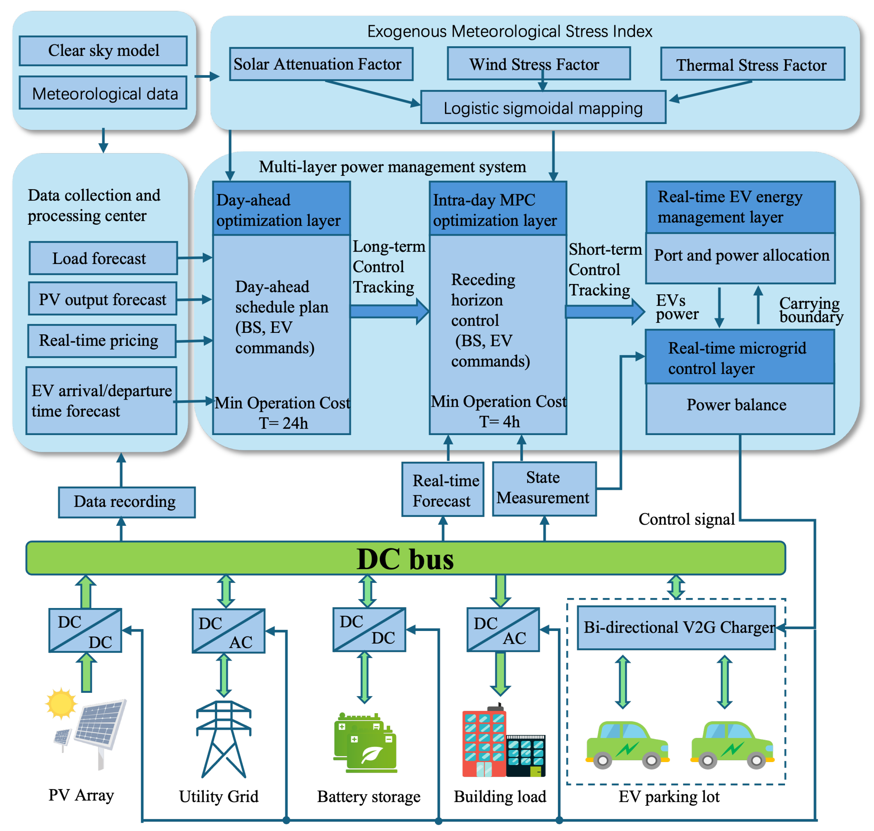
Figure 2.
Scenario generation framework.
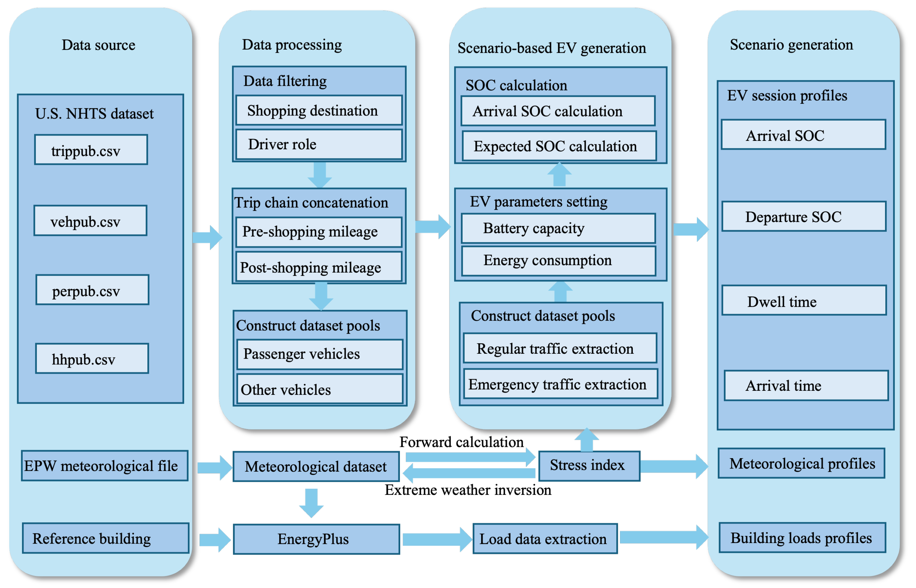
Figure 3.
Weather and building data on a typical summer day: (a) Weather data. (b) Building demand profile.
Figure 3.
Weather and building data on a typical summer day: (a) Weather data. (b) Building demand profile.
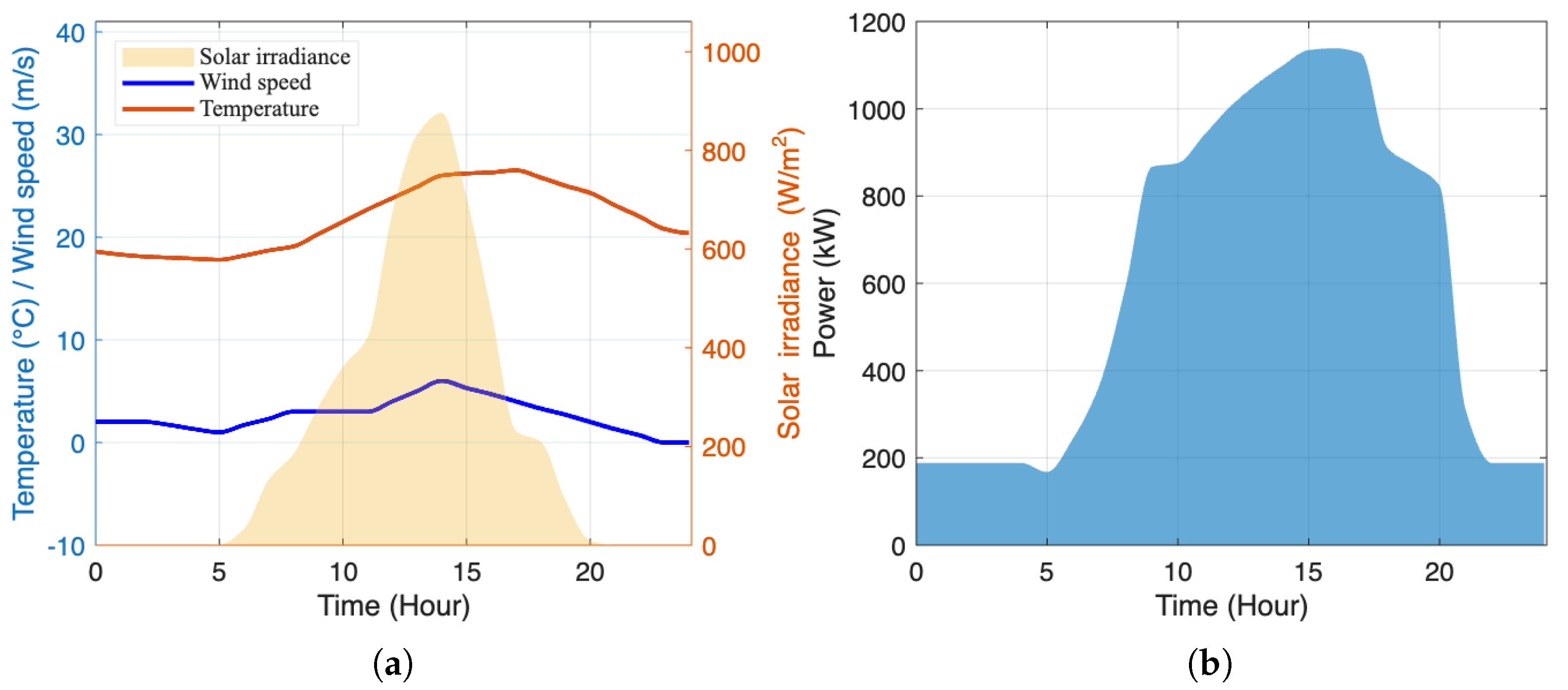
Figure 4.
EVs data on a typical summer day: (a) EVs’ arrival SOC and expected departure SOC. (b) EVs’ arrialtime and dwelltime.
Figure 4.
EVs data on a typical summer day: (a) EVs’ arrival SOC and expected departure SOC. (b) EVs’ arrialtime and dwelltime.
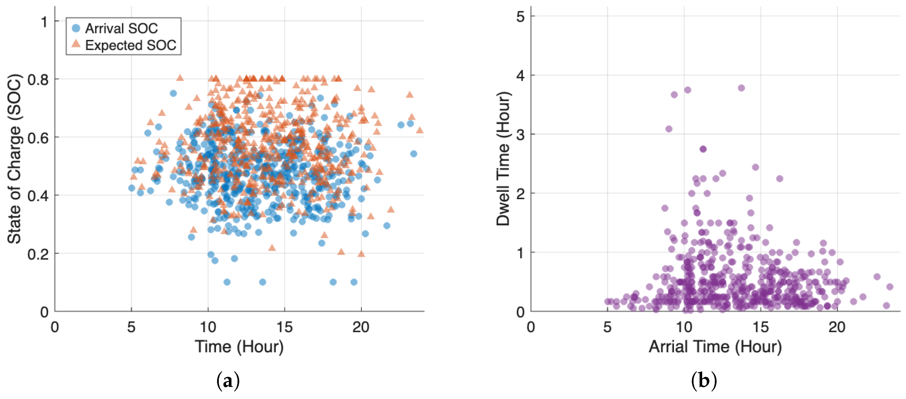
Figure 5.
Experimental results of strategy 5: (a) Power curves. (b) BESS state. (c) EVs traffic flow. (d) Driver satisfaction.
Figure 5.
Experimental results of strategy 5: (a) Power curves. (b) BESS state. (c) EVs traffic flow. (d) Driver satisfaction.
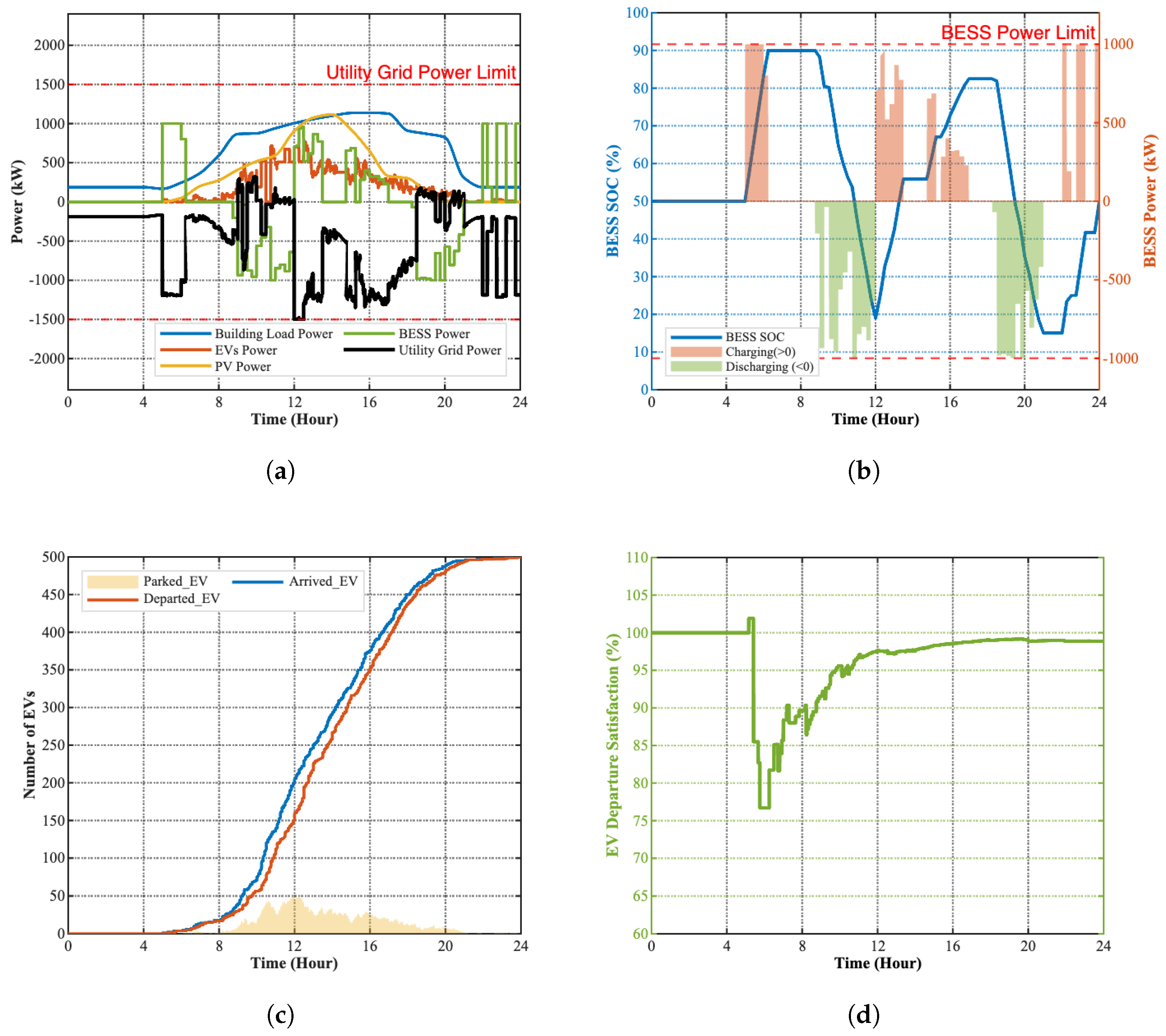
Figure 6.
Experimental results under extreme weather: (a) Stress index comparison. (b) Stress index penalty coefficients. (c) EVs SOC comparison. (d) BESS SOC comparison.
Figure 6.
Experimental results under extreme weather: (a) Stress index comparison. (b) Stress index penalty coefficients. (c) EVs SOC comparison. (d) BESS SOC comparison.
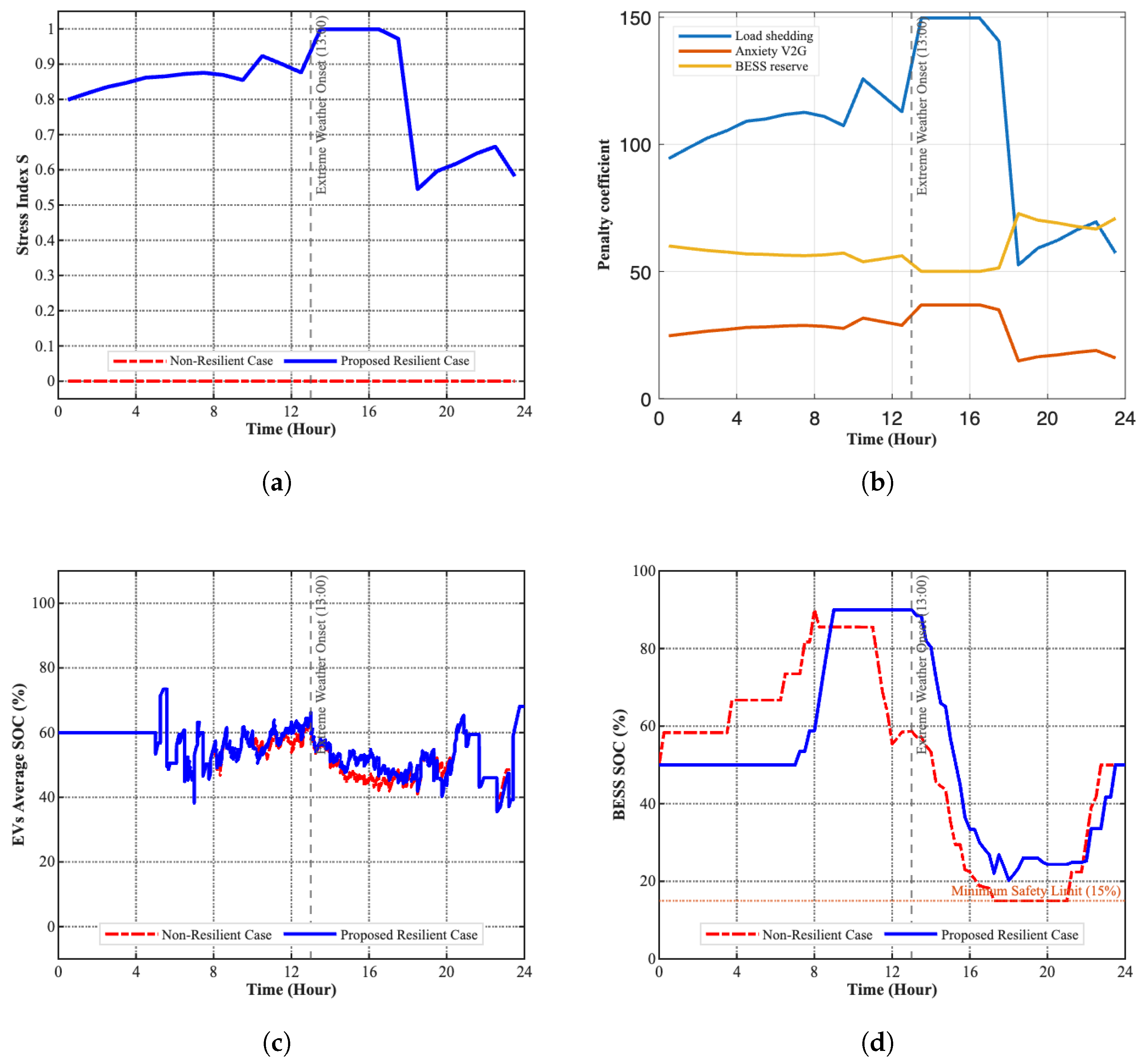
Figure 7.
Experimental results on sensitivity to : (a) Stress index under varying . (b) Operating cost and pre-disaster SOC at 13:00 under varying . (c) BESS SOC trajectory comparison. (d) EVs and BESS simulation results comparison.
Figure 7.
Experimental results on sensitivity to : (a) Stress index under varying . (b) Operating cost and pre-disaster SOC at 13:00 under varying . (c) BESS SOC trajectory comparison. (d) EVs and BESS simulation results comparison.
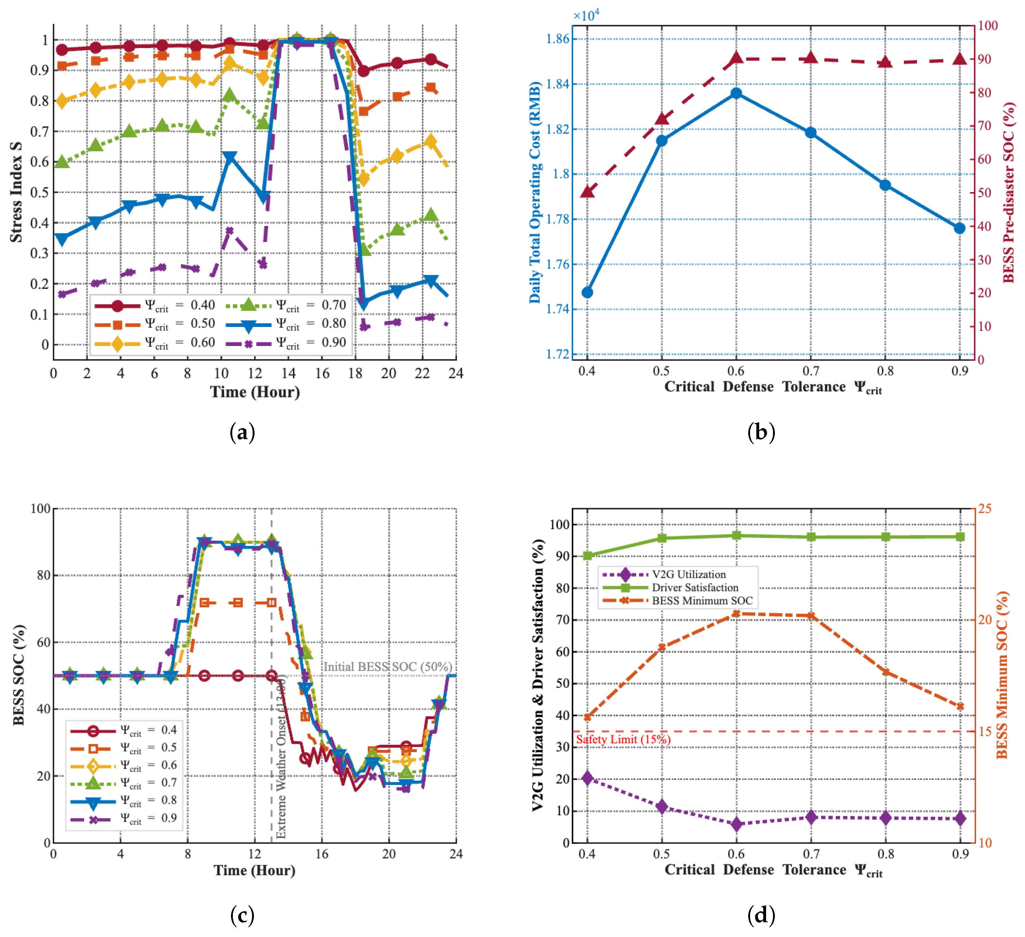
Figure 8.
Experimental results on sensitivity to : (a) Driver satisfaction and V2G energy utilization under varying . (b) EV fleet V2G power comparison.
Figure 8.
Experimental results on sensitivity to : (a) Driver satisfaction and V2G energy utilization under varying . (b) EV fleet V2G power comparison.
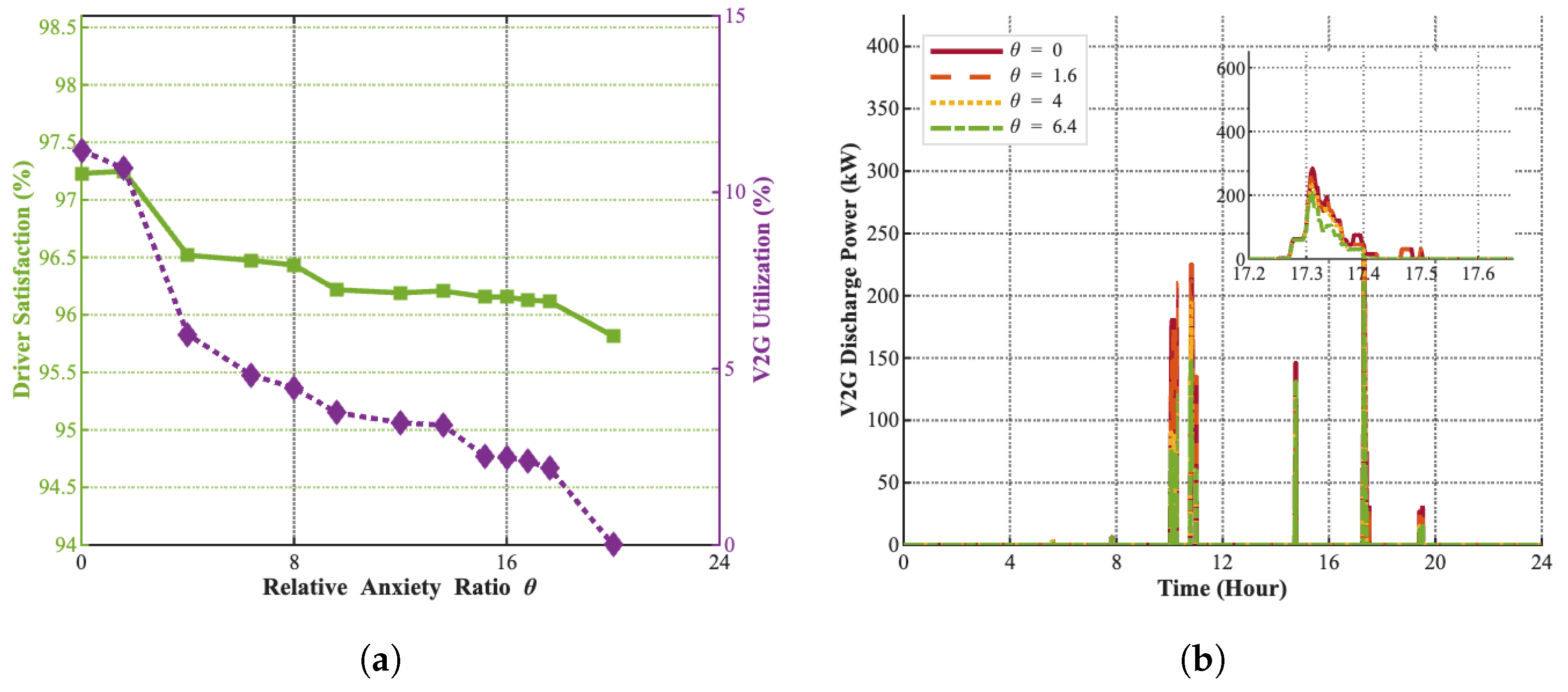

Table 1.
System configuration and the sizing parameters.
| Parameter | Value | Parameter | Value |
|---|---|---|---|
| 1.5MW | 30% | ||
| 3MWh | 50% | ||
| 1MW | 1.5MW | ||
| 15% | N | 100 | |
| 90% | 95% |
Table 2.
Economic penalty and electricity tariff parameters.
| Parameter | Value | Parameter | Value | Parameter | Value |
|---|---|---|---|---|---|
| 15 RMB | 5 | 0.3 | |||
| 2.3 | 0.134 RMB/kWh | 0.35 | |||
| 4 | 0.268 RMB/kWh | ||||
| 2 | 0.18 RMB/kWh | ||||
| 100 | 0.6 | ||||
| 0.5 | 10 | 5 m/s | |||
| 10 | 0.35 | 20 m/s |
Table 3.
Performance comparison under typical summer scenario.
| Strategy | Total cost (RMB) | Grid trading cost (RMB) | Degradation cost (RMB) | Load security (%) | Driver satisfaction (%) | V2G utilization (%) |
|---|---|---|---|---|---|---|
| 1 | 11749.94 | 10765.66 | 984.27 | 100 | 100 | 0.00 |
| 2 | 4701.65 | 3850.70 | 850.95 | 100 | 3.3 | 506.46 |
| 3 | 11172.18 | 8910.99 | 2261.19 | 100 | 90.14 | 0.00 |
| 4 | 11183.69 | 9152.64 | 2031.05 | 100 | 97.41 | 26.92 |
| 5 | 10938.06 | 8693.81 | 2244.25 | 100 | 99.20 | 15.57 |
Table 4.
Performance comparison under extreme winter scenario.
| Scenarios | Total cost (RMB) | Grid trading cost (RMB) | Degradation cost (RMB) | Load security (%) | Driver satisfaction (%) | V2G utilization (%) |
|---|---|---|---|---|---|---|
| Non-Resilient | 16317.52 | 14380.97 | 1936.56 | 100 | 92.70 | 43.25 |
| Resilient | 18359.54 | 16443.40 | 1916.14 | 100 | 96.52 | 5.97 |
Disclaimer/Publisher’s Note: The statements, opinions and data contained in all publications are solely those of the individual author(s) and contributor(s) and not of MDPI and/or the editor(s). MDPI and/or the editor(s) disclaim responsibility for any injury to people or property resulting from any ideas, methods, instructions or products referred to in the content. |
© 2026 by the authors. Licensee MDPI, Basel, Switzerland. This article is an open access article distributed under the terms and conditions of the Creative Commons Attribution (CC BY) license (http://creativecommons.org/licenses/by/4.0/).
Copyright: This open access article is published under a Creative Commons CC BY 4.0 license, which permit the free download, distribution, and reuse, provided that the author and preprint are cited in any reuse.


