

Submitted:
17 June 2026
Posted:
22 June 2026
You are already at the latest version
Abstract
In the linear approximation of general relativity, the field and force equations are transformed into vector equations with forms identical to covariant Maxwell and Lorentz force equations and are benchmarked to known strong-field solutions. The transformed equations can be used to: Apply aspects of electromagnetism theory and electrodynamics to weak-field gravitation; design laboratory tests of general relativity at high speeds; and characterize more accurately the coalescence of compact binaries. If linearized gravitation is treated as a vector field, one consequence is that ordinary quadrupole radiation from a rotating binary is found to be a linear superposition of Doppler-modulated dipole gravitational waves from each mass. Dipole waves at the orbit frequency may be observable in the merger event GW150914 at about 0.5 percent of the power and 7 percent of the strain amplitude. Another consequence is a cosmic gravitational background (CGB) much like the cosmic microwave background. The CGB relates the Hubble constant to Planck’s constant at an equilibrium temperature of about 20 to 22 K. An exact solution of Einstein’s equation for a static universe with a CGB accounts for the Hubble redshift, mature galaxies at high redshifts, and the appearance of cosmic acceleration in SN-Ia supernova light curves.
Keywords:
linearized general relativity
; covariant vector-field gravitation
; dipole gravitational waves
; cosmic acceleration
; cosmic gravitational background
; lambda-cold-dark-matter model
1. Introduction
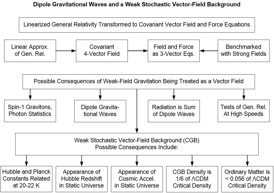
This paper on dipole gravitational waves and a weak stochastic gravitational vector-field background:
- Transforms linearized field and force equations into covariant vector equations;
- Explores consequences of weak-field gravitation being treated as a vector field;
- Finds radiation from a rotating binary to be a linear superposition of dipole waves;
- Can be used to characterize mergers of compact binaries more accurately;
- Explores properties and consequences of a weak stochastic vector-field background.
The linearized equation of motion is one of the most underutilized tools of general relativity. This paper transforms this covariant-tensor equation into a form that has been familiar for more than a century, that of the covariant-vector equation of motion of a charged particle in an electromagnetic field. In many respects this unique transformation allows more than a century of development of electromagnetism theory and electrodynamics to be applied directly to weak-field gravitation.
In fully nonlinear general relativity, gravitational fields, including gravitational wave fields, have energy density, and therefore possess gravitational mass. Fields and radiation gravitate just as particle masses do. It is this gravitation of fields that causes general relativity to be a nonlinear theory that must be described by rank-2 tensor equations, rather than a linear vector theory, like electromagnetism.
In the linear approximation of general relativity, the gravitation of fields is negligible, and only masses gravitate. Fields and radiation do not gravitate. The linear approximation therefore allows gravitation to be described by linear vector-field equations, just as electromagnetism is. Section 2, “Method,” transforms the covariant rank-2 tensor equation of motion and the field equation of general relativity in the linear approximation to vector equations identical to the manifestly covariant form of the Lorentz force equation and the Maxwell field equations.
The linear approximation of general relativity is applicable when gravitational fields are weak. Then the gravitation of the fields may be ignored. An isolated mass is considered to have a weak gravitational field at a range when its gravitational potential is much less than , where and are the gravitational constant and the speed of light. For example, the gravitational field of the Sun is weak even at its surface, where the potential is about .
The gravitational field of the Sun is not weak, however, with respect to planetary orbits. The specific kinetic energy of planets in bound orbits, , is of the same order as the gravitational potential of the central mass. That means the linear approximation of general relativity cannot be used to calculate departures from Keplerian elliptical orbits, such as the precession of bound elliptical orbits around a central mass.
On the other hand, the linear approximation does apply to unbound flyby orbits for which the gravitational potential is much less than the specific energy of the particle, and the deflection of the particle is small. Section 3.1, “Gravitational impulse of a particle in uniform motion,” uses the linearized vector-field equation of motion to calculate the small deflection of particles flying by a much larger central mass for which . As long as this weak-field condition is satisfied, the small deflection in the vector field is valid for all particle velocities up to and including the speed of light.
The inapplicability of the linear approximation to the precession of planetary orbits helps explain why Einstein skipped over development of the linear vector theory of general relativity, and developed it first as a nonlinear tensor theory instead. The only astronomical observation available to Einstein at the time, against which he could benchmark his incipient theory, was the precession of Mercury’s orbit. As soon as he was able in 1915 to benchmark his nonlinear tensor field equation to the observed precession of Mercury’s orbit, he confidently published the results, citing precession of Mercury’s orbit as supporting evidence.
A few years later, further support was given to general relativity by observations of the deflection of starlight about the Sun’s limb during a total eclipse. But calculation of deflection of starlight requires only a linear approximation and a vector theory. What if the deflection of starlight had been the only astronomical observation available to Einstein, against which he could benchmark his incipient theory? Then it is reasonable to suppose that Einstein would have developed general relativity first as a covariant vector theory of gravitation, corresponding to the covariant vector theory of electromagnetism that he himself had promulgated earlier.
Table 1 shows what general relativity might have looked like if Einstein had developed it first as a covariant vector theory, neglecting the nonlinear gravitation of fields. Table 1 highlights the analogies between vector-field electromagnetism and vector-field gravitation in the linear approximation. All the notation in Table 1 will be defined later in this paper. The table is presented here to give a preview of how the linear approximation of general relativity in its vector formulation so closely corresponds to electromagnetism. But another reason the table is presented here is to make a clear distinction up front between the mass that is the source of the gravitational fields and the test mass that observers use at their location to measure the gravitational fields. The source mass has 4-velocity . The test mass has 4-velocity . This distinction of notation is maintained throughout the paper.
From the debut of the exact fully nonlinear tensor theory of general relativity, the linearized vector theory and concomitant dipole gravitational fields and waves have been largely overlooked, if not disdained. Many reasons are given for this neglect. One reason cited more than others is the notion that conservation of momentum rules out dipole gravitational waves.
Many textbooks, for example [1,2,3,4], correctly maintain that in a closed system the total momentum of all masses, fields, and radiation is conserved. That means that the second time derivative of the total mass dipole moment of all masses, fields, and radiation in a closed system is zero. Since the second derivative of the dipole moment is the source of dipole radiation, the argument goes that there can be no dipole radiation from such a closed system. This argument is made, for example, in [1] on page 189.
It is technically correct that the total mass dipole moment of all masses, fields, and radiation in a closed system does not accelerate. One cannot conclude from this, however, that a system of interacting masses does not produce dipole gravitational waves and radiation at points of observation within the system.
No system of dynamically interacting masses is a closed system. Every system of interacting masses produces gravitational radiation that carries linear and angular momentum and energy away from the masses at the speed of light. The mass dipole moment of the remaining masses, excluding fields and radiation, accelerates when the masses radiate momentum asymmetrically. In the linear approximation, it is this acceleration of the mass dipole moment of the interacting masses, excluding fields and radiation, that produces dipole gravitational radiation.
If the accelerating dipole moment of interacting masses, excluding fields and radiation, is a source of dipole gravitational radiation, then this dipole radiation should be observable in the signals detected by gravitational wave observatories from the merger of compact binaries. And indeed, this dipole radiation is observable.
In a surprising validation of the vector formulation of the linear approximation of general relativity, this paper shows that dipole radiation is exactly equivalent to the ordinary gravitational radiation from rotating quadrupoles. That is, what we call quadrupole radiation is the superposition of dipole waves.
Section 3.2, “Dipole radiation from a rotating binary,” shows that the ordinary gravitational radiation emitted by a rotating quadrupole actually comprises interfering dipole gravitational waves from each of the rotating masses individually. Because one of the masses of the binary is moving towards the detector while the other is moving away, there is a difference in frequencies of the dipole waves observed from each of the masses at the detector, a difference that repeats twice per orbit. The resulting interference of the dipole waves from each of the masses produces gravitational radiation that has exactly the same metric, frequency, angular power distribution, and total power as ordinary quadrupole radiation. Section 3.3, “Dipole radiation fields, polarization, and power,” derives the properties of these vector dipole gravitational waves, closely corresponding to the properties of vector dipole electromagnetic waves.
Interfering dipole gravitational waves are equivalent to ordinary quadrupole waves only for well-behaved binaries, like binary pulsars essentially in steady state. For well-behaved binaries, the interference of dipole waves from each of the masses is nearly complete, leaving only the higher-order quadrupole waves at twice the orbit frequency to propagate to detectors.
In contrast, mergers of compact binaries are highly nonlinear events. The nearly complete interference of the dipole waves in the radiation zone is disrupted by the strong gravitational fields in the source region. This nonlinear disruption of interference can lay bare some of the dipole wave radiation at the orbit frequency.
Section 3.4, “Strain waveform model for GW150914,” analyzes an unfiltered strain waveform from the first detected merger of black holes, the merger event known as GW150914. Ordinarily, only the quadrupole radiation at twice the orbit frequency and at higher frequencies are of interest, and lower frequencies are filtered out to clean up the signal. For example, more than half of the power at the orbit frequency was filtered out of the strain signal from GW150914 that was cleaned up for publication. Section 3.4 shows that the unfiltered strain signal from GW150914 has a Fourier component at the orbit frequency that is of the order of 7 percent of the total strain amplitude, corresponding to a dipole radiation power of order 0.5 percent of the total power.
With the aid of numerical relativity, dipole-wave signals at the orbit frequency from mergers of compact binaries can be analyzed and related to the nonlinear effects within the source region that disrupted their interference at the detector. Data from the many dozens of detections of such mergers that have already been compiled at gravitational-wave observatories should be sufficient to support or to disprove the existence of dipole gravitational waves. Then, by analyzing dipole waveforms at the orbit frequency, laid bare by nonlinear disruptions of dipole-wave interference, much additional information can be gleaned for more accurately characterizing merger events.
Whether gravitational radiation from a rotating binary is considered to comprise dipole waves from each of the masses interfering or quadrupole waves from the binary makes no difference in the total power radiated from well-behaved binaries or in the strain signals from compact binary mergers, aside from small nonlinear disruptions. But there is a major physical difference between the two possibilities, a difference that has far-ranging implications.
Classical quadrupole gravitational waves, the kind that have been theorized since 1916, do not apply forces to particles. Instead, they cause spacetime coordinates to fluctuate past particles. That is, particles initially at rest remain at rest in a quadrupole gravitational wave. By contrast, dipole gravitational waves push and pull particles, just as dipole electromagnetic waves push and pull charged particles. At a gravitational wave observatory, the strain signals look the same, but there is a big difference physically and conceptually.
Because dipole gravitational waves do not just cause coordinates to oscillate past particles, but apply actual physical forces to the particles themselves, even an isolated particle, which emits no quadrupole radiation, can be a source of dipole gravitational radiation.
A dipole gravitational wave incident on an isolated particle will cause the particle to oscillate, just as a dipole electromagnetic wave incident on an isolated charged particle will cause the charged particle to oscillate. The isolated charged particle accelerated by an electromagnetic wave has an accelerating mass dipole moment. Of course, the change of momentum of the particle is exactly compensated by the scattered electromagnetic wave. But the oscillating charged particle radiates its own Larmor radiation independently of the scattered electromagnetic wave.
The same is true of a dipole gravitational wave causing an isolated particle to oscillate. The oscillating particle has an accelerating mass dipole moment. The change of momentum of the particle is exactly compensated by the scattered dipole gravitational wave. But the oscillating particle radiates its own dipole gravitational radiation in accordance with the covariant vector formulation of the linear approximation of general relativity, as shown in Table 1.
Section 3.5, “Scattering of dipole gravitational waves,” calculates scattering cross sections for dipole gravitational waves incident on isolated particles and on resonant mass oscillators, as also shown in Table 1.
The calculation of dipole gravitational wave scattering cross sections in Sec. 3.5 is just one example in this paper of how aspects of electromagnetism theory and electrodynamics can be applied to weak-field gravitation. The total scattering cross section for scattering of unpolarized dipole gravitational radiation by an isolated particle is analogous to the Thomson cross section for scattering of unpolarized electromagnetic radiation by an isolated charge. Similar analogies between vector-field electromagnetism and vector-field gravitation in the linear approximation are highlighted in Table 1.
The close correspondence of the covariant vector-field formulation of general relativity in the linear approximation to the covariant vector-field formulation of electromagnetism suggests that gravitation might be fundamentally a vector field. And tensor-field general relativity might be just the nonlinear generalization of vector-field gravitation that includes the gravitation of fields. Similarly, vector-field electromagnetism can have a nonlinear generalization to tensor-field equations when dealing with certain anisotropic and nonlinear media, for example.
The vector-field formulation of the linear approximation of general relativity is supported in this paper by multiple examples of benchmarking of the linearized results with the fully nonlinear strong-field theory. Examples that lend support to the vector-field formulation of general relativity in this paper include:
- The transformation of the linearized field and force equations to manifestly covariant vector forms identical to covariant Maxwell and Lorentz force equations;
- Derivation of the weak gravitational vector field of a particle in arbitrary motion up to the speed of light, which generalizes the Hilbert force on particles moving radially in a static Schwarzschild field, and which is repulsive at radial speeds above ;
- The known unbound orbits of particles in a Schwarzschild field, when Lorentz-transformed to an inertial reference frame in which the source of the Schwarzschild field is moving with uniform velocity and in which the orbiting particle is instantaneously at rest, show that the forces on the particles agree;
- The exact strong field of a spherical mass in uniform motion is identical in the weak-field limit to the vector gravitational field;
- The deflection angle of particles passing through a weak gravitational field at all particle velocities, including the speed of light, agrees with the vector-field impulse calculation;
- The metric, frequency, angular power distribution, and total power of dipole gravitational radiation calculated from vector fields agrees exactly with ordinary quadrupole radiation from well-behaved rotating binaries.
Roughly the first half of Sec. 3, “Results,” deals with vector forces and dipole gravitational waves, as outlined above. The second half deals with a stochastic background of dipole gravitational radiation that is similar to the stochastic background of dipole electromagnetic radiation known as the cosmic microwave background (CMB).
Dipole electromagnetic waves cause charged particles to oscillate, and oscillating charges produce dipole electromagnetic radiation. The universe is an ensemble of charged particles oscillating in response to stochastic electromagnetic radiation, and these oscillating particles in turn produce their own electromagnetic radiation to add to the stochastic background. This background of stochastic electromagnetic radiation in equilibrium with charged particles is known as the cosmic microwave background. The CMB can be thought of as an ensemble of massless spin-1 bosons called photons obeying Bose-Einstein quantum statistics with an unspecified number of particles at an equilibrium blackbody temperature.
Similarly, dipole gravitational waves cause particles to oscillate, and oscillating masses produce dipole gravitational radiation. It is reasonable to consider the universe to be an ensemble of particles oscillating in response to stochastic dipole gravitational radiation, and in turn producing their own gravitational radiation to add to the stochastic background. This postulated background of stochastic gravitational radiation is named in this paper the cosmic gravitational background, or CGB. Just like the CMB, the CGB can be thought of as an ensemble of massless spin-1 bosons, in this case gravitons, obeying Bose-Einstein quantum statistics with an unspecified number of particles at an equilibrium blackbody temperature.
Section 3.6, “Quantization and statistics of the CGB,” derives the quantum statistical properties of the CGB in close correspondence with the CMB, supposing both to be ensembles of spin-1 bosons obeying photon statistics, though not at the same equilibrium temperature. Section 3.7, “Stochastic fields of the CGB,” derives the properties of the fluctuating gravitational fields of the CGB from Nyquist relations.
Just as the stochastic electromagnetic fields of the CMB produce a drag force on charged particles moving through the CMB, the stochastic gravitational fields of the CGB should produce a drag force on all particles moving through the CGB. Section 3.8, “Drag on particles in the CGB,” calculates the effects on particle motion, from slow speeds to ultrarelativistic, of the stochastic fields of the CGB.
To consider the cosmological implications of a CGB, this paper utilizes what may be the simplest and most featureless cosmological model of all, the static, homogeneous universe known as the Einstein universe, named for its first proponent. This model is an exact solution of the fully nonlinear Einstein equation. But the coordinates used for the metric of this cosmological model in this paper are uniquely simple. Through a mathematical sleight of hand, flat Cartesian coordinates eliminate the nonphysical mathematical singularity at the origin in anisotropic spherical coordinates of a static universe, and the spacetime curvature of the metric is entirely manifested as a time-dilation function. Section 3.9, “Exact metric of a static, homogeneous universe,” derives this metric and characterizes its properties.
With this simple model of a static universe, Sec. 3.10, “Redshift of light in a static universe,” calculates the effects of a static, homogeneous distribution of energy density throughout a static universe on propagation of light. The spacetime curvature of the metric, manifested as a time-dilation function, fully accounts for the Hubble redshift in a static universe.
It makes sense that the curvature of the universe alone should be able to fully account for the Hubble redshift, even in a static universe that is not expanding. When light propagates past a central mass like the Sun, the central mass delivers an attractive transverse impulse to the light. By conservation of momentum, the light delivers an equal and opposite attractive impulse to the central mass, imparting a kinetic energy to the central mass. A simple estimate of the energy that must be delivered by light to all the mass in its past light cone shows that the light must lose energy at about the rate of the Hubble redshift in a static universe.
The exact metric derived in Sec. 3.9 of a static universe also predicts a drag force acting on all particles moving through the static universe. The drag force is similar to the gravitational force on a particle climbing out of a gravitational potential, but by symmetry the energy is nonrecoverable when the direction of the particle through the static universe is reversed.
Section 3.11, “Particle motion in a static universe,” combines the effects on particle motion of the time-dilation effects of the metric of a static universe in Sec. 3.10 with the effects of CGB drag. Section 3.11 calculates the drag effects on particle motion and the energy dissipation caused by interaction of particles with the CGB.
Section 3.12, “Appearance of cosmic acceleration in a static universe,” offers another example, besides the Hubble redshift, suggesting that the cosmological model of a static universe may be of more than just pedagogical significance. The model of a static, homogeneous universe derived in Sec. 3.9 has only one parameter, the energy density. With only this one free parameter, the model gives a good fit of the distance modulus of Type Ia supernovas (SN-Ia) to the light-curve data. By contrast, the standard spatially-flat lambda-cold-dark-matter (ΛCDM) cosmology uses six parameters to fit the distance modulus of SN-Ia to the light-curve data.
Another intriguing result of Sec. 3.12 is that the model of a static universe with a CGB supports the observation that the baryonic matter density of our universe is much less than the ΛCDM critical density, , without needing to invoke dark mass or dark energy or even more than one adjustable parameter. As shown in Sec. 3.12, the best fit of the distance modulus of Type Ia supernovas (SN-Ia) to the light-curve data in a static universe occurs for a ratio of total energy density to ΛCDM critical density in the narrow range . Section 3.12 also suggests the energy density of the CGB in a static universe might be , leaving about for ordinary baryonic matter.
Section 3.13, “Hubble constant, drag constant, dipole anisotropy, and CGB,” relates recent measurements of the Hubble constant to the time-dilation factor derived in Sec. 3.10 and to the temperature of the CGB. The energy density of the CGB depends on its equilibrium temperature to the fourth power and depends on Planck’s constant through the Stefan-Boltzmann law.
Together, these dependencies on temperature relate the cosmological Hubble constant to the quantum mechanical Planck’s constant. Depending on the value of the Hubble constant, the equilibrium temperature of the CGB is predicted to be about 20 to 22 K.
The CGB might be expected to exhibit a dipole anisotropy, just as the CMB does. Section 3.13 calculates the magnitude of the dipole anisotropy of the CGB that is expected if the CGB shares the same rest frame as the CMB.
Section 3.14, “Quantum oscillators in the CGB,” suggests through several means that the stochastic vector fields of the CGB might underlie stochastic mechanics and the Schrödinger equation. Unlike quadrupole gravitational waves, which leave at rest particles that are initially at rest, the stochastic dipole gravitational waves of the CGB apply physical forces to particles. Unlike the stochastic electromagnetic fields of the CMB, the stochastic gravitational fields of the CGB apply stochastic forces to all particles, not just charged particles. Because the equilibrium temperature of the CGB, about 20 to 22 K, is much greater than the 2.7-K temperature of the CMB, and the energy density of the CGB is up to about 4,000 times greater than that of the CMB, the CGB dominates the stochastic mechanics of the CMB for free particles and resonant oscillators.
If the CGB is a collection of indistinguishable, massless, spin-1 bosons obeying photon statistics, then the stochastic dipole gravitational fields of the CGB will cause every particle, bound and unbound, to undergo stochastic motion, even in its lowest energy state. The calculation in this paper of the mean energy of mass oscillators closely follows the derivation of the mean energy of oscillators from the generalized Nyquist relations.
Lending support to the possibility that the stochastic vector fields of the CGB might be the “hidden variable” that underlies stochastic mechanics and the Schrödinger equation are these observations:
- The stochastic vector fields of the CGB apply physical forces to particles, and do not merely move coordinates past particles;
- The CGB vector fields are truly random, but with a root-mean-square deviation that is constant throughout a homogeneous universe;
- The CGB vector fields act the same on charged and uncharged particles;
- The energy density of the CGB dominates the energy density of the CMB by a factor up to about 4,000;
- Planck’s constant is related to the Hubble constant through the equilibrium temperature, which is constant throughout a homogeneous universe.
The results of this paper suggest that the concept of the Einstein static universe, which was largely abandoned in the 1930’s, may deserve a fresh look. The time-dilation effect of the metric of a static universe, when combined with the existence of a CGB, accounts fully for:
- The Hubble redshift in a static universe;
- The appearance of cosmic acceleration in SN-Ia light curves in a static universe;
- A baryonic matter density of the order of 5 percent of the ΛCDM critical density;
- A relationship of the cosmological Hubble constant to the quantum mechanical Planck’s constant through the equilibrium temperature of the CGB.
The covariant formulation of linearized gravitation in 4-vector notation is useful for much more than just applying aspects of electromagnetism and electrodynamics to weak-field gravitation. It is also ideal for designing new classes of laboratory tests of general relativity at high velocities. And it can be used to analyze the dipole gravitational waves produced by the accelera ting mass dipole moment of inspiralling compact binaries to supplement diagnostics for more accurate characterization of the sources.
Some of the usual objections that are raised against vector-field gravitation and dipole gravitational waves are addressed in this paper. This introduction has already addressed the existence of an accelerating mass dipole moment, and Sec. 3.2 presents a vivid demonstration that gravitational waves from rotating quadrupoles are in fact dipole waves from each of the masses interfering with each other. A few other objections are addressed in the paragraphs below.
For example, objections to one particular formulation of a vector gravitational field are raised in [2] on page 179. The vector gravitational field in this example is derived from a Lagrangian proposed by analogy with the Lagrangian of electromagnetism. A result of this particular formulation is that vector gravitational waves carry negative energy.
Unlike this example from [2], the vector gravitational field equations of this paper are not derived from some ad hoc Lagrangian. Instead, they are derived in Sec. 2 from the standard Lagrangian of general relativity in the linear approximation and from a covariant transformation to a form identical to Maxwell’s field equations. Since the vector field equations have the identical form as Maxwell’s equations, it is no surprise that vector gravitational waves carry positive energy. In fact, Sec. 3.2 shows that vector gravitational waves carry the same energy from rotating binaries as predicted by general relativity.
Another objection concerns radiative degrees of freedom. Under the usual set of constraints on the linearized perturbation metric , the only radiative degrees of freedom are those that allow conventional transverse-traceless (TT) quadrupole gravitational waves to propagate in vacuum with their two independent polarizations. Under a different set of constraints, equally valid, very different radiative degrees of freedom are allowed.
For example, in [5], a gauge-invariant formalism was introduced that fully characterized the degrees of freedom of linearized gravity. Applying the Hilbert gauge condition (also known as the Lorenz gauge) and imposing a set of five constraints on the perturbation metric completely fixes all the local gauge freedom. The five constraints used in [5] are , zero trace, and . When the gauge conditions are fixed in this way, then the only physical radiative degrees of freedom allowed are the TT quadrupole waves. The non-TT components of the metric do not exhibit radiative degrees of freedom. These five constraints are conventionally chosen only because they are convenient, not because they are necessary [5].
But imposing these particular constraints eliminates dipole gravitational waves ab initio. Section 3.2 shows that the components are precisely the ones that give rise to TT dipole gravitational waves propagating as physical vector waves. With a different set of constraints imposed on the metric, the radiative degrees of freedom allow dipole gravitational waves to propagate as vector waves in vacuum, carrying energy and momentum with transverse polarizations, just as electromagnetic waves do. Section 3.2 shows, in fact, that the metric of dipole gravitational waves from a rotating binary, interfering in the radiation zone, is identical in the Hilbert gauge to the metric of gravitational radiation from the rotating quadrupole in the same gauge.
Section 3.2 further shows that dipole gravitational radiation not only can be produced, but must be produced, by every dynamic gravitational interaction. Every interaction of two masses, whether gravitationally bound or unbound, results in an acceleration of the local mass dipole moment, generally, if not always, in a direction opposite the instantaneous velocity of the lighter mass. In the linear approximation, the local mass dipole moment includes only the masses that are the sources of the radiation, not the equivalent mass of the radiation itself. Dipole radiation is produced by this acceleration of the local mass dipole moment.
Attempts to cast linearized general relativity into Maxwellian form can present pitfalls. In [6], it was shown how the coordinate freedom of linearized general relativity can lead to coordinate choices that produce unphysical “Maxwellian mirages.” Past attempts to mold both the field equations and force equation of linearized general relativity into Maxwellian form have often led to mistakes in ordering choices. In such attempts, the linearized gravitational field equations might be cast in the form of Maxwell equations, but the form of the force equation would differ from the Lorentz force equation, or vice versa [6].
Section 2.1 avoids such pitfalls and “Maxwellian mirages,” as were identified in [6], by maintaining strict covariance in the transformations that cast both the field equations and force equation of linearized general relativity into Maxwellian form. No ordering choices are made other than those imposed initially by the linearization. The vector gravitational waves that emerge from the covariant transformations are not mirages, but are real, physical transverse waves, just as electromagnetic waves are, carrying energy and momentum to the radiation zone.
The results of these covariant transformations speak for themselves. The covariant vector field and force equations are benchmarked to the well-known cases of exact strong-field solutions listed above. Section 3.1 illustrates the utility of the linearized vector equation of motion in this new formalism by the ease with which the small deflection of an unbound particle in a static field is calculated, not just at the Newtonian limit and at the speed of light, but at all speeds in between.
Using a vector-field equation of motion, this paper derives the gravitational field of a particle moving with arbitrary relativistic velocity and acceleration exactly within the linear approximation of general relativity. This equation of motion in 3-vector notation has much greater applicability and analytic utility than all earlier formulations.
Earlier calculations of the gravitational fields of moving particles were done for slow velocities of source masses and test masses [2,3,7,8,9,10,11] and exactly for relativistic velocities of a stationary spinning mass [2,3,12,13] and of a mass in uniform motion [14,15]. Hilbert discovered that a particle with a radial speed exceeding is repelled even in a weak static Schwarzschild field [16]. Subsequent papers addressed [17] and reviewed [18] the critical speed for repulsion of particles moving radially in a Schwarzschild field and along the rotation axis of a spinning source [19]. Hilbert’s results were generalized to arbitrary particle trajectories and velocities in a weak Schwarzschild field [15] using a Liénard-Wiechert “retarded solution” approach [20] and benchmarked to known special cases of strong fields and relativistic velocities [15,21].
This paper explores the linearized equation of motion of general relativity in original ways. The approach yields substantial results that are novel, and even surprising. The detailed, step-by-step derivations of the results are presented in 25 appendices, summarized as follows.
Appendix A, “Covariant Vector Equation of Motion,” transforms the linearized (weak-field) equation of motion of general relativity to a form identical to the covariant Lorentz force equation of electromagnetism.
Appendix B, “Covariant Vector Gravitational Field Equation,” transforms the linearized tensor field equation of general relativity to a vector field equation in a form identical to the covariant Maxwell equations of electromagnetism, and derives the general solution of the vector field equation for a point-mass source.
Appendix C, “Gravimagnetic and Relativistic Gravitational Forces,” derives the linearized weak-field equation of motion in 3-vector notation for two special cases: Slow source and slow test mass; and relativistic source and stationary test mass. The gravitational force in 3-vector notation of a relativistic mass on a stationary test mass resembles the electric force in 3-vector notation of a relativistic charge on a stationary charge, but with important differences, differences that allow Hilbert gravitational repulsion of masses at relativistic speeds, for example.
Appendix D, “Velocity Field of Relativistic Particles,” gives the exact gravitational field in the linear approximation of a particle in arbitrary relativistic motion. This velocity field is benchmarked to three well-known strong-field cases: Hilbert repulsion; the field of a spherical mass in uniform motion; and unbound orbits in the Schwarzschild field of a source moving with uniform velocity.
Appendix E, “Gravitational Impulse of a Particle in Uniform Motion,” calculates the gravitational impulse delivered to a test mass by a particle in uniform motion. As a fourth benchmark of the velocity field derived in App. D, the general formula is derived for the small deflection of an unbound particle in the weak field of a much larger mass for all impact parameters and from slow Newtonian velocities to the speed of light.
Appendix F, “Quadrupole Radiation from a Rotating Binary,” reviews the common derivation of gravitational waves produced by a well-behaved rotating quadrupole. In App. H, these quadrupole gravitational waves will be shown to be a linear superposition of dipole waves.
Appendix G, “Acceleration Field of Relativistic Particles,” derives the exact gravitational field in the linear approximation of an accelerating particle with arbitrary velocity in the radiation zone of the particle.
Appendix H, “Dipole Radiation from a Rotating Binary,” derives the angular power distribution of gravitational radiation and the total power radiated by a rotating binary in a manner entirely different from the common derivation reviewed in App. F. Owing to a Doppler modulation effect, the dipole waves from each of the masses of a binary do not completely interfere. The superposed dipole waves from each of the masses of a binary have the same metric and same angular power distribution as the quadrupole waves that were reviewed in App. F. But the dipole waves accelerate masses in accordance with the force equation of App. C, and do not merely produce curvature ripples on a flat spacetime background.
Appendix I, “Dipole Vector Gravitational Field of a Rotating Binary,” derives the superposed dipole vector gravitational field of a rotating binary in the radiation zone in the transverse gauge and shows that it is the plane-wave vector-field solution of the covariant vector gravitational field equation derived in App. B. The superposed dipole vector fields of each of the masses of the binary appear the same to a gravitational-wave detector as the quadrupole tensor field.
Appendix J, “The Polarization and Power of Vector Gravitational Plane Waves,” presents a general treatment of the polarization and power of dipole vector-field plane-wave solutions of the gravitational field equation in the slow-source linear approximation. Even though dipole vector fields accelerate masses, and do not merely produce curvature ripples on a flat spacetime background, a gravitational-wave detector makes no distinction in the linear approximation. In the linear approximation, the perturbation metrics satisfying the Hilbert gauge condition of the dipole vector-field and quadrupole tensor-field plane-wave solutions of the field equation are identical. Nonlinear events, however, like the compact-binary mergers detected at gravitational-wave observatories, can reveal dipole gravitational radiation at the orbit frequency, as discussed in App. L.
Appendix K, “Dipole Radiation from an Isolated Mass Dipole,” calculates in general the gravitational field and angular distribution of dipole radiation from an isolated accelerating mass dipole, corresponding to the Larmor electromagnetic dipole power radiated by an isolated accelerating electric dipole. In the linear approximation, only masses gravitate, not radiation or fields. A free particle accelerated by a field radiates as an isolated mass dipole. Dipole gravitational radiation is calculated for the specific example of a mass caused to move in a circular orbit, for example, by a continuous circularly polarized wave, such as an electromagnetic wave or a dipole gravitational wave.
Appendix L, “Strain Waveform Model for Merger Event GW150914,” estimates the dipole radiation power at the fundamental orbit frequency produced nonlinearly by the specific merger event, GW150914. The dipole gravitational waves from each of the masses of a well-behaved binary, produced at the orbit angular frequency, interfere almost completely, resulting in an interference waveform at twice the orbit frequency. The events detected at gravitational wave observatories are generally highly nonlinear mergers of massive compact binaries. The dipole waves from each of the masses are distorted and delayed by the strong gravitational fields of their companions. These nonlinear effects within the source region disturb the linear interference of the waveforms and leave a trace signal at the orbit frequency. The model suggests that dipole waves at the orbit frequency may be observable in the event GW150914 at about the 0.5-percent power level.
Appendix M, “Scattering of Dipole Gravitational Waves by a Free Particle,” calculates the total cross section for scattering of unpolarized dipole gravitational radiation by free particles, corresponding to the Thomson cross section for scattering of unpolarized electromagnetic radiation by free charges.
Appendix N, “Scattering of Dipole Gravitational Waves by a Mass Oscillator,” calculates the total cross section for scattering of unpolarized dipole gravitational radiation by oscillators. The line width of dipole gravitational radiation from oscillators at resonance is also calculated.
Appendix O, “Quantization and Statistics of the Cosmic Gravitational Background (CGB),” calculates the properties of a cosmic gravitational background (CGB), assuming it is a collection of spin-1 bosons in thermal equilibrium obeying photon statistics. Every accelerating mass produces dipole gravitational radiation, causing stochastic dipole gravitational fields to be as ubiquitous throughout the universe as stochastic electromagnetic fields in the cosmic microwave background (CMB).
Appendix P, “Fluctuating Gravitational Fields of the CGB from Nyquist Relations,” calculates the mean energy density of the stochastic vector gravitational fields of the CGB in thermal equilibrium. The calculation is based on an extension of the Nyquist relation for voltage fluctuations in electrical impedances, and gives the same dependence of energy density on dipole gravitational fields as is derived in App. K.
Appendix Q, “Drag on Particles in the CGB,” calculates the dipole gravitational radiation and the dissipative deceleration of particles moving through the CGB and acted on by no forces other than the dipole gravitational forces produced by the stochastic gravitational and gravimagnetic fields of the CGB. The dissipative drag force on particles exerted by the CGB is similar to the dissipative drag force exerted on charged particles by the CMB. But unlike the CMB, the CGB affects the energies of particles significantly only over cosmological distances.
Appendix R, “Exact Metric of a Static, Homogeneous Universe,” summarizes the derivation of an exact solution in isotropic Cartesian coordinates of Einstein’s equation for a static (time-independent and time-reversible), homogeneous spacetime. Through a mathematical sleight-of-hand, spurious nonphysical singularities are eliminated and the spacetime curvature is manifested only in the time coordinate of the diagonal metric as a time-dilation function.
Appendix S, “Hubble Redshift and Apparent Cosmic Acceleration in a Static Universe,” calculates from the metric in App. R the effects of a static, homogeneous distribution of energy density throughout a static universe on propagation of light. The spacetime curvature of a static universe causes a time dilation of clocks increasing with their distance that accounts for the Hubble redshift and for an apparent cosmic acceleration. As shown in App. U, the appearance of cosmic acceleration in a static universe fits Supernova Type Ia (SN-Ia) light curve data well for a narrow range of possible energy densities in the static universe.
Appendix T, “Particle Motion in a Static Universe With CGB Drag,” calculates the combined effects on particle motion of time dilation derived in App. S with the dissipative drag force of the CGB. With respect to the rest frame of a static universe, the CGB causes a deceleration of all particles proportional to the root-mean-square gravitational field of the CGB. This dissipative drag force of the CGB is identified in this appendix with the ostensibly nondissipative time-dilation drag force of the metric. Then the equation of motion of particles in a static, homogeneous universe relates the Hubble constant to .
Appendix U, “Appearance of Cosmic Acceleration in a Static Universe,” calculates the effects in a static universe on SN-Ia light curves of the time dilation calculated in App. S. The effects give a reasonably good fit to the light-curve data in a model of a static homogeneous universe. The model has only one adjustable parameter, total energy density, and the fit to the SN-Ia light-curve data is best over a range of densities from about 0.21 to 0.22 times the ΛCDM critical density.
Appendix V, “Hubble Constant, Drag Constant and CGB Temperature,” summarizes some of the recent results of measurements of the Hubble constant and relates those measurements to the scalar deceleration constant from App. Q and to the temperature of the CGB.
Appendix W, “Dipole Anisotropy of the CGB,” calculates the dipole anisotropy of the CGB temperature assuming it has the same source as the dipole anisotropy of the CMB, the velocity of our solar system with respect to the background.
Appendix X, “Hubble Constant Related to Planck’s Constant by the CGB,” relates the Hubble constant to the energy density of the CGB and, through the equilibrium temperature of the CGB, relates the Hubble constant to Planck’s constant, assuming the CGB is a collection of spin-1 bosons in thermal equilibrium obeying photon statistics. The range of possible values of the Hubble constant suggests possible values of the equilibrium temperature of the CGB of about 20 to 22 K.
Appendix Y, “Mean Energy of an Oscillator in the CGB,” calculates the mean energy of a resonant oscillator in the CGB at an equilibrium temperature. An oscillator is driven by the stochastic vector fields of the CGB and its motion is damped by dipole radiation produced by its own acceleration. The calculation closely follows the derivation of the mean energy of oscillators from the generalized Nyquist relations in App. P.
Each of these 25 appendices supports the results presented in specific sections of the paper. Table 2 is a guide relating specific appendices to the specific sections they support.
2. Method
This section transforms the field and force equations of general relativity in the linear approximation to forms corresponding to the covariant field and force equations of electromagnetism. Then the covariant equations are expressed in familiar 3-vector notation to facilitate derivation of the results of Sec. 3, “Results.”
Section 2.1, “Covariant vector field and force equations,” transforms the covariant rank-2 tensor field equation and equation of motion of general relativity in the linear approximation to vector equations identical to the manifestly covariant form of the Maxwell field equations and the Lorentz force equation. Appendices A and B give the detailed derivation of the transformations.
Section 2.2, “Linearized 3-vector force equation,” with Apps. C and D derives the general force equation in the linear approximation of general relativity in a 3-vector form that is particularly useful for calculating the results of Sec. 3.
2.1. Covariant vector field and force equations
The metric tensor is linearized as , where is the Minkowski metric tensor of flat spacetime, and is the perturbation metric tensor. The linear approximation neglects all terms of order , including interactions of source masses with their own fields and with their own radiation, and including terms of order times test-mass acceleration.
From the Euler-Lagrange equation, the equation of motion of a test mass in a weak external field is, from [3] and App. A,
(1)
where is the velocity 4-vector of the test mass; is the Lorentz relativistic factor; is the proper time interval; and partial derivatives are indicated by .
With the definitions of a coupled 4-vector potential, , an antisymmetric gravitational field tensor, , and a coupled velocity 4-vector, , App. A shows that the covariant equation of motion of a test mass in a weak gravitational field takes on the familiar form, shown in Table 1, of the covariant Lorentz force equation for a charged particle in an electromagnetic field,
(2)
or here the covariant vector gravitational force equation in the linear approximation.
With a transformed perturbation metric tensor defined as , where is the trace of , the Hilbert gauge condition is , and the field equation in the Hilbert gauge is , where is the energy-momentum tensor [3]. Appendix B shows the step-by-step transformation of this tensor field equation to the vector field equation,
(3)
where is the coupled current density 4-vector, and is the trace of .
The vector field equation in the Hilbert gauge, Eq. (3), has a form identical to the electromagnetic field equation in the Lorentz gauge, as shown in Table 1. As shown in App. B, the solution through invariant Green functions, treated in [22] and in many books on quantum field theory, such as [23], can be written as
(4)
where is the displacement vector from the source position to the test mass at , and . The delta function involving the retarded time, , provides the retarded behavior demanded by causality [22]. The covariant equation of motion, Eq. (2), and wave equation, Eq. (3), with its solution, Eq. (4), which all have forms identical to their electromagnetic-field counterparts, can be used to solve for the relativistic motion in the linear approximation of a test mass for a source with any energy-momentum tensor.
The energy-momentum tensor of a particle alone, not including its gravitational field, is , where is the rest-mass density of the particle and is its rest mass; is its velocity 4-vector; and is its Lorentz factor [3]. For this point-mass source, the mass current density in the linear approximation is , where , as derived in App. B. The velocity 4-vector of the particle source and the velocity 4-vector of the test mass are coupled in the velocity 4-vector as a necessary step in the transformation of the equation of motion from a tensor equation to a covariant vector equation.
Using the mathematical procedures from electromagnetism [22], integration over in Eq. (4) yields the “retarded solution,”
(5)
where ; is a unit vector pointing from the source to the test mass; is the displacement vector from the source to the test mass; and the brackets mean that the quantity inside the brackets is evaluated at the retarded time . The retarded 4-vector potential is related to the retarded perturbation metric by , so that . Just as for the electromagnetic Lorentz force, the covariant gravitational equation of motion, Eq. (2), is written in Table 1 in the form of a three-dimensional force equation,
(6)
where and are components of the 4-vector potential , and is the coupled momentum 3-vector.
2.2. Linearized 3-vector force equation
The derivation of the linearized 3-vector force equation in this section is detailed in Apps. C and D.
In terms of the linearized perturbation metric , the three space components of the equation of motion of the test mass, Eq. (1), are
, (7)
where ; for ; and .
An illustration of “gravimagnetic” induction effects on a slowly moving test mass by a slowly moving source is commonly made [3] by ignoring terms of second order in test mass velocity and by ignoring time derivatives and in Eq. (7), as shown in App. C.
A much more interesting and useful special case of Eq. (7) is to allow arbitrary relativistic motion of the source and to observe the test mass in its own initial rest frame. For this special case, which is explored in the following sections, and initially, and the force equation, Eq. (7), becomes
(8)
This force equation has the form of a gradient of a scalar plus a partial time derivative of a 3-vector, similar to the Lorentz force equation of an electric field on a charged particle at rest. In terms of the retarded solution, Eq. (5), of the vector field equation of a particle in arbitrary relativistic motion, Eq. (8) becomes
(9)
as derived in App. C.
From the detailed derivation in App. D and references therein, the gravitational field on a test particle at rest of a particle mass in arbitrary relativistic motion from Eq. (9) becomes
(10)
where .
Evaluating the derivatives in Eq. (10), as detailed in App. D, gives the relativistically exact (weak) retarded gravitational field of a source mass with arbitrary velocity on a test mass instantaneously at rest at the spacetime point as
,(11)
where an overdot indicates a derivative with respect to retarded time, such as .
The gravitational field in Eq. (11) comprises a so-called “velocity field” and an “acceleration field” , as [15]. Just as in electromagnetism [22], the velocity field is independent of acceleration of the source mass and falls off with distance as . The acceleration field depends linearly on acceleration of the source mass and falls off as . In the linear approximation, Eq. (11) is the most general expression for the combined velocity field and acceleration field of a particle in arbitrary relativistic motion on an initially stationary test mass.
The acceleration field is negligible in the source region of a gravitational field and for all cases of uniform motion of the source, because in these cases. The acceleration field in the transverse gauge will be used in Sec. 3 to calculate the properties of dipole gravitational waves in the radiation zone of the source and properties of the cosmic gravitational background (CGB) of stochastic vector-field gravitational waves. The acceleration field is benchmarked by showing in App. H that it correctly predicts all the properties of gravitational radiation from a well-behaved rotating binary.
The velocity field can be used to calculate weak-field relativistic gravitational effects in the source region, such as deflection of particles in fly-by orbits and Hilbert repulsion of particles at source speeds above . The velocity field in Eq. (11) is benchmarked to weak-field deflection of particles at all velocities in Sec. 3.1 and in App. E. And the velocity field in Eq. (11) has been benchmarked to these three well-known strong-field cases:
- The Hilbert repulsive force on particles in a strong Schwarzschild field [16];
Equation (11) generalizes the Hilbert force on particles in a static Schwarzschild field. Hilbert found that a particle moving at speeds above , radially inwards or outwards, in the static field of a central mass appears to a distant observer to be repelled by the central mass [16]. Hilbert’s result applies even to strong gravitational fields, but only for radial motion of the particle. Equation (11) generalizes Hilbert’s result to particle motion in all directions, not just radial, but only for weak gravitational fields. From Eq. (11), the threshold condition for repulsion of a particle at rest in any direction is [15,21].
For a radially incoming particle of mass and uniform velocity, the gravitational field on a test mass at rest, from Eq. (11) and App. D, is
(12)
where is the range of the particle at the retarded time that the field was created at the source, not the time that the field was detected at the test mass. For a radially outgoing particle, the gravitational field on a test mass at rest is
(13)
The fields of both the radially incoming and outgoing particles in Eqs. (12) and (13) exhibit Hilbert repulsion at particle speeds above , but the repulsive field of an incoming ultrarelativistic () particle is a factor stronger than that of an outgoing particle.
The coordinate transformations from retarded (primed) coordinates to isotropic (present) coordinates for particles in uniform motion are given in [15]. In terms of the range of the particle at the present time of detection of the field at the test mass, the fields in Eqs. (12) and (13) are the same,
(14)
for both radially incoming and outgoing particles, in agreement with Hilbert’s result for weak fields [16].
The exact time-dependent field solution of Einstein’s gravitational field equation for a spherical mass moving with arbitrarily high constant velocity was reviewed in [15]. The solution is essentially that of a Schwarzschild field in uniform motion. This exact dynamic field solution was calculated from an exact metric first derived, but not analyzed, in [14]. This exact strong field of a spherical mass in uniform motion (that is, constant ) was shown through a coordinate transformation [15] to be identical in the weak-field limit to Eq. (11).
An even more general benchmark for Eq. (11) is found in [21]. The exact unbound orbit of a particle of mass in the strong Schwarzschild field of a mass is calculated by Chandrasekhar [13]. A simple Lorentz transformation from the rest frame of to the initial rest frame of gives the Lorentz-transformed unbound orbit of in the strong field of the mass in uniform motion. Equation (11) is benchmarked by showing in [21] that the Lorentz-transformed unbound orbit of in the weak field of the mass in uniform motion corresponds to the force on predicted by Eq. (11).
Potential applications of Eq. (11) have been proposed and analyzed. For spacecraft propulsion, a suitably large mass approaching faster than the Hilbert repulsion threshold can quickly propel a heavy payload from rest to relativistic speeds, in some cases even faster than the approaching mass, with negligible stresses on the payload [15,21].
Immediate applications of Eq. (11) include laboratory tests of general relativity at ultrarelativistic speeds. In 1977, Braginsky, Caves, and Thorne were the first to propose measuring the relativistic gravity of proton bunches circulating in storage rings using a crystal detector resonant at the bunch frequency [7]. They outlined an experiment for the 1-TeV POPAE storage ring that was proposed for Fermilab at the time, and concluded that such an experiment “does not seem unreasonable” [7].
The POPAE, later dubbed the Tevatron, was operational at Fermilab from 1983 to 2011, but this experiment was not done. Perhaps if Eq. (11) had been available earlier, showing that the experiment proposed by [7] could have resulted in the first detection of the repulsive gravitational field predicted by Hilbert, the incentive to do such an experiment on the Tevatron would have been greater.
Today an experimental test of Eq. (11) at ultrarelativistic speeds, very much like the one proposed in [7], can be performed next to the beamline of the Large Hadron Collider (LHC) with a high-Q acoustic detector resonant at the proton-bunch frequency [15,24]. This tabletop experiment to detect repulsive gravity requires hours of continuous operation of the LHC, but can be conducted at any point along the ring without interfering in any way with the normal operations of the LHC. Because the 7-TeV LHC is a much more powerful storage ring than the Tevatron was, such an experiment is much more reasonable. For example, the quality factor of the crystal detector need only be about 1012 [15], rather than the needed for the Tevatron [7].
The vector gravitational field embodied in Eq. (11) can be tested not just at ultrarelativistic velocities, but at mechanical speeds up to the order of sound speeds in solids. At high mechanical speeds, a test of the gravitational fields predicted by Eq. (11) can be performed on an existing flywheel, such as the NASA G2 Flywheel Module [25] with a modified rotor, which can produce a post-Newtonian dc bias signal at a gradiometer up to about 10–12 s–2 [24].
3. Results
3.1. Gravitational impulse of a particle in uniform motion
This section summarizes the calculation in App. E of the gravitational impulse delivered to a test mass by a particle in uniform motion at any speed. The derivation of the velocity field in 3-vector notation of a particle in arbitrary relativistic motion, Eq. (11), was given in Apps. C and D.
Using Eq. (11), App. E shows that the transverse specific impulse delivered to a test mass by a particle of mass in uniform motion with constant momentum and impact parameter is
(15)
where is the component of the velocity field normal to the trajectory of the mass .
Since the transverse impulse, , delivered to a test mass is equal and opposite to the impulse delivered to the particle, the angular deflection of the particle in the weak field of the test mass , for and , from Eq. (15), is
(16)
The angular deflection in Eq. (16) agrees with the angular deflection of light, for , and agrees with the angular deflection of a slow particle, for , and agrees with the same result calculated by other means in [2] on page 671, thereby providing further benchmarking for Eq. (11).
3.2. Dipole radiation from a rotating binary
This section begins by reviewing the common derivation of quadrupole gravitational waves produced by a rotating binary, as detailed in App. F and as presented, for example, in [1,2,3,4]. The interpretation of these waves is that they carry energy and momentum, but do not accelerate masses. Instead, these waves are believed to be curvature ripples on a flat spacetime background that cause coordinates to oscillate past masses, but do not cause the masses themselves to accelerate.
Then this section summarizes the detailed derivation in App. G of the exact linearized gravitational acceleration field in the transverse gauge of a relativistic particle in the radiation zone.
Finally, this section shows by the detailed derivation in App. H that the superposition of dipole gravitational waves in the radiation zone from each of the masses of a binary has exactly the same angular power distribution as the quadrupole radiation. That is, the quadrupole radiation from a rotating binary is just the superposition of dipole waves from each of the masses.
In this section and in App. H, these quadrupole gravitational waves will be shown to be a linear superposition of dipole waves. Owing to a Doppler modulation effect, the dipole waves from each of the masses of a binary do not completely interfere. At any moment, the frequency of the dipole waves from the mass approaching the detector is slightly higher than the frequency of dipole waves from the other mass. The superposition of the dipole waves from each of the masses has the same metric and same angular power distribution as the quadrupole wave from the binary, but the dipole waves do accelerate masses in accordance with the force equation. The strain signal at a gravitational wave detector, however, is the same.
The first detections by gravitational-wave observatories, such as the Laser Interferometer Gravitational-Wave Observatory (LIGO), of the gravitational waves produced by coalescing compact binaries heralded the advent of a new era of gravitational-wave astronomy. These detections have conclusively established the existence of the gravitational waves first predicted by Einstein over a century ago. At the low-frequency end of the observable spectrum of strain signals from these detections, waiting to be uncovered by detailed numerical simulations, may lie evidence of dipole gravitational waves as well. This evidence for the existence, or nonexistence, of dipole gravitational waves has been available in the data accumulating from the many dozens of detections of compact binary coalescences since 2015.
Highly nonlinear, relativistic, strong-field events, like the coalescence of massive black holes, are expected to produce dipole gravitational radiation at much higher levels than well-behaved binaries, like binary pulsars. And not just because the acceleration of the local mass dipole moment is much greater. Nonlinear alterations of the waves in the strong-field source region, including frequency and phase shifts at the source, can disrupt the interference of the dipole waveforms from each of the masses. When the source region is strongly altered in ways like this, powerful dipole radiation can be produced even by sources that have very little dipole moment. That nonlinear imprint on the dipole waveforms is what makes dipole gravitational radiation such a potentially valuable diagnostic tool in helping to characterize the coalescence of compact binaries.
Figure 1 shows a configuration for calculating the quadrupole radiation of a well-behaved binary system comprising two particles of masses and moving in circular orbits with constant angular frequency and constant speeds and , respectively, about their center of mass.
The retarded coordinates of and , respectively, from Fig. 1, are
(17)
where and are the constant orbital radii of and , respectively.
As reviewed in App. F, in the linear approximation, the field equation in the Hilbert gauge, , for the perturbation metric tensor and the energy-momentum tensor , has the exact solution for masses rotating in circular orbits in the x-y plane,
, (18)
where ; is the reduced mass of the binary comprising masses and moving in circular orbits with constant angular frequency and with constant distance between the masses; and are the polar and azimuthal spherical coordinates; and is the retarded time.
From App. F, the quadrupole power per unit solid angle radiated from this binary in the radial direction is
(19)
(20)
In Apps. G and H, the metric in Eq. (18), angular power distribution in Eq. (19), and total radiation power in Eq. (20) of a well-behaved binary rotating in circular orbits are all derived in a very different way, from considering the interference of dipole gravitational waves from each of the masses of the binary.
In the radiation zone where , the velocity field in Eq. (11) is negligible and the force on a test mass at rest is that of the acceleration field in Eq. (11) alone. The trace of the perturbation metric components of the field of a relativistic point-source mass is , where is the scalar range to a test mass , as derived in App. G. In the radiation zone, is approximately constant on a time scale of a wave period, so in the radiation zone. And since , then on a time scale of a wave period in the radiation zone, and the transverse gauge, also known as the Coulomb gauge, is applicable [22].
From App. G, the perturbation-metric component , , in the radiation zone of a relativistic particle with 4-velocity , is
(21)
where the scalar quantity is a retarded Lorentz-transformed range from source to test mass; is the range from the source at to the test mass at ; ; is a unit vector pointing from source to test mass; and all quantities within the brackets are evaluated at the retarded time .
From Apps. G and H, the perturbation-metric component , , at a stationary test mass in the radiation zone of a particle of mass in arbitrary relativistic motion is
(22)
where is the k-component, , of the local mass dipole moment of the particle.
From Eq. (22) and App. H, the perturbation-metric components , , in the radiation zone of the rotating binary system of particles shown in Fig. 1, with masses and moving in constant circular orbits, are
(23)
where and are the k-components of the dipole moments of and , respectively; and are the Doppler factors; and are the 4-velocities; and and are the constant Lorentz factors of and moving in circular orbits.
The metric components of the binary in Eq. (23) are linear superpositions of the components of each of the masses of the binary individually. The Doppler factors and in Eq. (23) modulate the dipole gravitational waves of each of the masses and prevent them from interfering completely, even though . The interference of these two dipole waves to second order in produces the quadrupole waves of a binary at third order in .
Appendix H shows that the perturbation-metric components , , from a superposition of dipole waves in Eq. (23) are identical to the perturbation-metric components , , from the quadrupole metric in Eq. (18). Since the perturbation-metric components , , are identical in Eqs. (18) and (23), by the Hilbert gauge condition, all the components of the superposed dipole waves are identical, as shown in App. H.
And since the metric of the superposed dipole waves is identical to the metric of the quadrupole wave, App. H shows that the angular power distribution and total power of the dipole radiation is identical to the angular power distribution and total power of the quadrupole radiation in Eqs. (19) and (20), as well.
Although the perturbation-metric components , , are identical for the superposed dipole waves of Eq. (23) and the quadrupole wave of Eq. (18), there is a significant physical difference. Equation (8) shows that the superposed dipole waves apply an actual physical force, , on the test mass , which is initially at rest, and do not merely cause coordinates to oscillate past the test mass.
Because every dynamic gravitational interaction of a mass quadrupole produces quadrupole radiation, no quadrupole is a completely closed system in the linear approximation. The acceleration of the local mass dipole moment is a second-order nonlinear effect of classical quadrupole radiation for all quadrupoles. Every binary has an accelerating center of mass and therefore an accelerating local mass dipole moment [26,27,28]. Gravitational waves carry linear momentum away from binaries in the instantaneous direction of velocity of the lighter mass because the angular distribution of gravitational radiation is more tightly focused in that direction [29,30]. Thorne reviewed the rate of momentum radiated by a binary, which is equal and opposite to the recoil force on the center of mass [31]. By integrating this recoil force, the final linear-momentum kick delivered to a binary after coalescence was estimated in [30,32].
In the linear approximation of general relativity, because only masses gravitate and radiation and fields do not, the gravitational field of any set of masses is just the linear superposition of the fields of each of the individual masses.
3.3. Dipole radiation fields, polarization, and power
This section summarizes the calculation in App. I of the dipole vector gravitational field in the radiation zone of a binary system of masses and rotating in circular orbits. It also summarizes the results of App. J in calculating the polarization properties of plane vector gravitational waves and their energy flux. Lastly, it summarizes the calculation in App. K of the dipole radiation emitted by an isolated mass dipole.
The dipole acceleration field in Eqs. (10) and (11) can be decomposed into a transverse component, , and a component parallel to , a unit vector in the direction of propagation, which vanishes in the radiation zone. From Eq. (10), the transverse dipole vector field in the radiation zone of a relativistic particle of mass is
(24)
as was displayed in Table 1.
The significance of Eq. (24) cannot be overstated. This equation is a quantitative statement of the sentence in the abstract of this paper: Every accelerating mass produces dipole gravitational waves that accelerate masses in the radiation zone.
The dipole gravitational acceleration field in the transverse gauge of the rotating binary shown in Fig. 1 at a stationary test mass in the radiation zone is calculated in App. I. If the dipole field propagating in the radial direction is taken to be the direction at the test mass, so that , then the gravitational field of the binary in the transverse gauge at the test mass in the radiation zone, from App. I, is
(25)
The dipole vector gravitational field, Eq. (25), is the plane-wave vector-field solution of the covariant-vector gravitational field equation, Eq. (3), for slow velocities of the binary shown in Fig. 1 and for the special case in Eq. (9) of a test mass at rest in the radiation zone.
As shown in Table 1, the “gravelectric” field in Eq. (24) is similar to the electric field of an electromagnetic wave. And just as the transverse magnetic field of an electromagnetic wave is related to the transverse electric field by , the transverse “gravi mag ne tic” field of a dipole gravitational wave is related to the transverse “gravelectric” field by .
In terms of the unit 4-vectors defined in App. J, , , , and , the wavenumber 4-vector of a free dipole gravitational plane wave propagating in the direction with angular velocity is , and the dipole-wave polarization vectors are and . The polarization tensors of a quadrupole plane wave are and . Like quadrupole waves, dipole gravitational waves are transverse, and carry momentum and energy, and cannot be made to vanish by a gauge transformation. But unlike quadrupole waves, the right-hand sides of Eqs. (24) and (25) do not vanish for dipole waves, because dipole waves physically push masses, and do not just push coordinates past masses.
The energy flux of a free dipole gravitational plane wave propagating in the direction, derived from the canonical prescription [3] and App. J, is
(26)
corresponding to Poynting’s vector of electromagnetism.
For the vector field of a binary, Eq. (25), the angular distribution of dipole power, calculated in App. J, is
(27)
and the total dipole power radiated continuously by the rotating binary, obtained in App. J by integrating over all solid angle, is
(28)
in agreement with the quadrupole radiation in Eq. (20).
Dipole gravitational radiation is not just emitted from all binaries, but from all gravitationally unbound mass quadrupoles as well [24,33]. When a mass flies past a much greater mass in the initial rest frame of with energy much greater than the gravitational binding energy, the static field of delivers a transverse impulse to the lighter mass. But the lighter mass delivers an equal and opposite impulse to , and an energy . The loss of at least an energy by decelerates . Within the linear approximation and the impulse approximation, App. E calculated and the angular deflection of for any velocity of by integrating the velocity field of Eq. (11) [15]. The deceleration of produces an acceleration of the local center of mass in a direction opposite the velocity of , thereby producing dipole gravitational radiation.
Since only masses gravitate in the linear approximation, and not radiation or fields, an isolated mass accelerated by a field radiates as an isolated mass dipole. Appendix K calculates the gravitational field and angular power distribution of dipole radiation from an isolated accelerating mass dipole in general, and then the radiation for the specific example of a mass caused to move in a circular orbit, for example, by a continuous circularly polarized wave, such as an electromagnetic wave or a dipole gravitational wave.
Appendix K shows that to lowest order in , the acceleration of a test mass at rest at in the source-free radiation zone, by a particle of mass moving with acceleration , is the dipole vector gravitational acceleration field in the transverse gauge,
(29)
where an overdot indicates a derivative with respect to retarded time .
Equation (29) is the nonrelativistic version of Eq. (24). An acceleration, , of a source mass anywhere in the universe produces an acceleration of a test mass at a range equal to the transverse component, , of the acceleration of the source, reduced by the factor , at a retarded time after the acceleration of the source.
Equations (24) and (29) make quantitative an effect discovered by Einstein two years before he finished formulating general relativity. In his 1913 letter to Mach, on page 544 of [2], Einstein referred to this effect as “dragging.” Wheeler [34] called this effect a manifestation of the principle, “Inertia here is ruled by mass there.” The Lense-Thirring effect is an example of this dragging effect for a rotating source [35].
From App. K, the dipole gravitational power radiated per unit solid angle by an isolated mass is
(30)
where is the instantaneous angle between and , a unit vector in the direction of propagation.
Integrating Eq. (30) over all solid angle gives the total instantaneous dipole power radiated into the radiation zone by the isolated nonrelativistic accelerated mass ,
(31)
where is the second time derivative of the mass dipole moment . As shown in Table 1, Eq. (31) corresponds to the familiar Larmor result for the total electromagnetic dipole power, , radiated by a nonrelativistic accelerated charge .
The total dipole power radiated by an isolated accelerated mass is of a sufficient order of magnitude to accelerate all the mass of a homogeneous static universe lying in the future light cone of the isolated mass in accordance with Eq. (29) [33].
For the specific case of an isolated mass moving with slow velocity in a circular orbit, App. K shows that the plane-wave vector field propagating in the direction in the transverse gauge at a test mass at rest in the radiation zone is
(32)
The vector field of the orbiting mass is plane polarized in the orbital plane (for ) and circularly polarized along the axis of the orbit (for ).
As shown in App. K, the dipole gravitational power radiated per unit solid angle by the isolated mass moving in a circular orbit is
(33)
and the total dipole power radiated continuously by the isolated mass in constant circular motion, obtained by integrating over all solid angle, is given by Eq. (31).
3.4. Strain waveform model for GW150914
This section presents a simple model, detailed in App. L, of the strain signal waveform produced by a merging compact binary. The model suggests that the unfiltered data from the first observed binary black-hole coalescence [36], GW150914, recorded by the Advanced Laser Interferometer Gravitational-Wave Observatory (LIGO) [37], is not inconsistent with a dipole strain signal at the orbit angular frequency of the order of 10 percent of the quadrupole signal at . That corresponds to a dipole power at of the order of 1 percent of the quadrupole power at .
Once the low-frequency end of the sensitivity band had been extended from 40 Hz to 10 Hz, Advanced LIGO was capable of observing the dipole strain signal from GW150914 [37]. But this section shows that most of the dipole radiation power at the orbit frequency was eliminated in post-processing of the signal by a bandpass filter from 35 to 350 Hz [36].
Section 3.2 and App. H showed that the quadrupole radiation from a well-behaved binary at is just the linear superposition of dipole waves from each of the masses at the orbit angular frequency . In a merger of a compact binary, this interference of dipole waves is disrupted by nonlinear effects, such as wavefront delays and distortions. Consequently, some of the dipole radiation can be detected at the orbit frequency.
To get a rough order-of-magnitude estimate of the dipole power that might be expected at the orbit frequency during the sudden final inspirals of binary systems of compact masses, like black holes and neutron stars, a simple waveform model is presented in this section. This model suggests that GW150914 marked not just the first direct detection of the quadrupole gravitational waves predicted by Einstein, but the first direct detection of dipole gravitational waves at the orbit frequency as well.
In the century since Einstein first predicted quadrupole gravitational waves [38,39], little attention has been paid to dipole gravitational waves and dipole gravitational radiation. A reason for this neglect is the common belief that the center of mass of any system of masses interacting only through gravitational forces must have zero acceleration, and that any such system having zero acceleration of its center of mass cannot produce dipole gravitational radiation. The discovery published in 1975 of the binary pulsar system PSR B1913+16 [40] and its nearly constant rate of energy loss through quadrupole gravitational radiation [41,42] did not increase expectations for ever being able to observe dipole gravitational radiation at the orbit frequency.
That situation changed dramatically on September 14, 2015, when Advanced LIGO made the first direct detection of gravitational waves [36]. The event known as GW150914, the orbital inspiral and coalescence of two black holes, resulted in a burst of gravitational radiation with an energy equivalent to 3 solar masses and a peak gravitational-wave luminosity of 3.6 × 1056 erg/s [36]. By comparison, ASASSN-15lh, the most luminous supernova yet found, had a bolometric luminosity of about [43].
In [36], the features of GW150914 inferred from the strain signals detected at Advanced LIGO are , , and an orbit frequency at peak amplitude of 75 Hz, so at peak amplitude. Blithely applying Kepler’s third law, , to this very non-Newtonian event gives the separation between the masses at peak amplitude as km. With these estimates and nonrelativistic formulas, the peak quadrupole gravitational-wave power radiated by the masses according to the nonrelativistic formula is W, which is close to the estimate of W made from fits to numerical simulations of peak gravitational-wave luminosity [36].
With such enormous power densities, strong fields, gross distortions of spacetime in the source region, and relativistic orbital velocities, nonlinear relativistic effects, like asymmetric radiation-reaction forces accelerating the center of mass, are expected to disrupt the interference of the dipole waves from each of the masses and to produce dipole gravitational radiation at the orbit frequency.
Modifications of the source region of a radiating system may reveal dipole radiation at the fundamental frequency, regardless of the dipole moment of the system. For example, a current loop with zero electric dipole moment was found to produce copious dipole electromagnetic radiation because part of the current loop was immersed in an overdense plasma that shielded part of the fields from leaving the source region [44]. Although the source had no dipole moment, source-region alteration by the plasma caused it to radiate as a dipole.
Similarly, any physical process that disrupts the interference of dipole gravitational waves coming from the source region can lay bare the interfering dipole gravitational waves at the orbit frequency. The nonlinear distortion and alteration of gravitational waves in the source region can disrupt gravitational wave interference in the radiation zone in some directions.
Nonlinear physical processes in the source region that can disrupt the complete interference of dipole gravitational waves in the radiation zone include the Shapiro or gravitational time-delay effect [45] and the gravitational lensing effect [46]. In general relativity and other metric theories of gravity, both of these effects apply equally to gravitational waves and electromagnetic waves.
Until 2019, all detected binary mergers had mass ratios consistent with unity [47]. That situation changed with the detection of a binary-black-hole coalescence with a mass ratio of [48]. This asymmetric coalescence, GW190412, carried clearly measurable signals not only at the dominant quadrupole frequencies, but for the first time at higher multipole frequencies as well. Asymmetric coalescences might also produce dipole radiation more abundantly. The advantages of modeling the higher multipoles of GW190412 were that the orientation of the binary was more accurately determined and tighter bounds were put on source parameters like the mass ratio and spin of the system [48]. Careful modeling of dipole radiation can offer the same advantages.
A principal value of carefully modeling dipole radiation from compact binaries is that it will enable more accurate determination of source parameters by a better matching of numerical relativity waveform templates to the observed time series data. Modeling dipole radiation will also lead to stronger tests of the validity of general relativity.
The following summarizes App. L, which shows how a simple waveform model can be used to estimate the dipole radiation power at the orbit frequency produced nonlinearly by the specific merger event, GW150914.
Figure 2 shows the unfiltered Advanced LIGO strain signal at the Hanford detector from the GW150914 event, adapted from [36]. The circles indicate eight consecutive positive-strain amplitude peaks during the final inspiral, which represent the “data” on which the simple waveform model is based. The dashed curve in Fig. 2(a) is the quartic-polynomial least-squares fit to these eight amplitude peaks. This least-squares-fit function, , is considered the envelope of the quadrupole signal amplitude in the waveform model.
Figure 2(a) shows an alternating pattern of amplitude peaks above and below the dashed least-squares-fit curve, which suggests that a dipole signal at the orbit frequency could be superposed on the quadrupole signal. The purpose of the strain waveform model is to estimate the possible order of magnitude of such a dipole signal relative to the quadrupole signal.
Dipole gravitational radiation is distinguishable from quadrupole radiation, in that the fundamental frequency is the orbit frequency of the binary, which is half the frequency of quadrupole radiation. Although much of the dipole wave signal at the orbit frequency is filtered out in post processing, the unfiltered data suggest that it may be detectable.
The dipole signal is modeled by a frequency equal to half the quadrupole wave frequency and by an amplitude envelope, , equal to the quadrupole amplitude envelope reduced by the constant factor . The model of the strain waveform of the superposed quadrupole and dipole waves is
, (34)
where is the time of the initial amplitude peak in Fig. 2.
The first term on the right-hand side of Eq. (34) represents the quadrupole wave and the second term represents the dipole wave. Here, is the quadrupole amplitude envelope, and the dipole amplitude envelope is taken to be , where . The quadrupole wave frequency, , is twice the orbit frequency, , and the dipole wave frequency is taken be equal to the orbit frequency.
The variance between the model waveform, Eq. (34), and the actual strain waveform is a minimum for . That is, the model waveform best fits the peak amplitudes of the Hanford LIGO strain signal from the GW150914 event for a dipole signal amplitude equal to 7.2 percent of the quadrupole signal amplitude. The improvement in the matching of the model with the strain signal by including a superposed dipole signal at is seen in the comparison of Figs. 2(a) and 2(b).
Figure 3 shows that the waveform model in Eq. (34), which includes a dipole wave, more closely fits the unfiltered strain amplitude peaks than no dipole wave for all dipole amplitudes up to about 14 percent of the quadrupole signal amplitude. Arbitrary choices were made in the selection of the strain signal waveform model. Nevertheless, a lesson that can be drawn from Fig. 3 is that a dipole gravitational wave at the orbit frequency with an amplitude of the order of 10 percent of the quadrupole gravitational wave is not inconsistent with the unfiltered strain signals from the event GW150914.
A bandpass filter of 35 to 350 Hz in post-processing of the GW150914 strain signals [36], however, removed most of the dipole signal. Figure 4(a) shows as dotted curves the model quadrupole and dipole waveforms of Eq. (34) for the best fit, . The solid curves in Fig. 4(a) are the same model waveforms after bandpass filtering of 35 to 350 Hz. The model quadrupole signal in Fig. 4(a) is barely affected by the filtering, while the dipole signal is badly distorted and diminished by the filtering.
This result is understood graphically by the power spectral density (PSD) of the model quadrupole and dipole waveforms in Fig. 4(b). The PSD of the model dipole waveform peaks below 35 Hz. Less than about 1 percent of the model quadrupole power is filtered out, while more than about half of the dipole power is filtered out. Integration of the PSD curves in Fig. 4(b) shows that the ratio of dipole to quadrupole power for before filtering is 0.52 percent and only 0.25 percent after bandpass filtering.
This section presented a simple waveform model of superposed dipole and quadrupole waves. When this waveform model is applied to the unfiltered strain signal data from the first observed merger event, GW150914, the model is consistent with dipole radiation power at about the 0.5 percent power level and a dipole signal amplitude for this event at about 7 percent of the quadrupole signal amplitude. The results of this model suggest that dipole gravitational radiation may already have been detected at about this power level in GW150914.
3.5. Scattering of dipole gravitational waves
The transformation of the linearized equation of motion of general relativity to the covariant-vector equation, Eq. (2), in many respects allows more than a century of development of electromagnetism theory and electrodynamics to be applied to weak-field gravitation. As one example bearing out this claim, this section calculates the scattering of dipole gravitational waves by free and oscillating masses in a manner analogous to the calculation of scattering of electromagnetic waves by free and oscillating charged particles.
This section summarizes the detailed calculation in App. M of the cross section for scattering of unpolarized dipole gravitational radiation by free particles, and the detailed calculation in App. N of the cross section for scattering by oscillators.
From the equation of motion of a free particle in the radiation zone of a slow accelerating mass, Eq. (29), and from the angular distribution of dipole gravitational power radiated by an isolated mass, Eq. (30), the differential scattering cross section for scattering of unpolarized dipole gravitational radiation by a free particle of mass is calculated in App. M as
(35)
where is the angle between the direction of propagation of the incident dipole wave and the scattered wave.
Integration of Eq. (35) over all solid angle gives the total scattering cross section for scattering of unpolarized dipole gravitational radiation by a free particle of mass as
(36)
The Thomson formula for scattering of unpolarized electromagnetic radiation by a free particle of charge and mass is just Eq. (35), with replaced by [22]. And the total electromagnetic scattering cross section, called the Thomson cross section, for scattering of unpolarized electromagnetic radiation by a free particle of charge and mass is also just Eq. (36), with replaced by [22].
Equations (35) and (36) apply to scattering of unpolarized dipole gravitational waves by free particles. The scattering of dipole waves by a resonant harmonic oscillator is calculated in App. N. The line width of the oscillators is calculated by taking the damping at resonance to be caused by reradiation.
From App. N, the total energy, kinetic plus potential, of an oscillator of mass and resonant angular frequency , driven by a dipole gravitational wave of constant amplitude and angular frequency , is
(37)
where is the damping constant determined by reradiation. From Eq. (37), the full width of the peak in the energy spectrum at half-maximum energy is the line width, , where the quality factor is .
Driven at resonant frequency, the oscillator acceleration is , and the total dipole power radiated from the oscillator in steady state, from App. N, is
(38)
From the reradiation of dipole power at resonance, App. N shows that the total scattering cross section for scattering of unpolarized dipole gravitational radiation by an oscillator at resonance is
(39)
which is times the scattering cross section of a free particle in Eq. (36). And the full-width-at-half-maximum (FWHM) line width of dipole gravitational radiation is
(40)
which is proportional to the “spring constant” of the oscillator.
3.6. Quantization and statistics of the cosmic gravitational background (CGB)
This section summarizes the results of App. O, which calculates the properties of the cosmic gravitational background (CGB) assuming it is a collection of spin-1 bosons in thermal equilibrium obeying photon statistics.
Every accelerating mass produces dipole gravitational vector fields in the radiation zone in accordance with Eq. (24) and, to lowest order in , with Eq. (29). And the dipole vector fields produced by every accelerating mass accelerate masses themselves in accordance with the linearized equation of motion. The ratio of the acceleration of a particle in the radiation zone to the acceleration of the mass at range that produced it is of order .
Dipole gravitational plane waves in the radiation zone have an energy flux given by Eq. (26), similar to the energy flux of Poynting’s vector of electromagnetism given by Eq. (J.10). And dipole gravitational fields have an energy density , similar to the energy density of electromagnetic fields.
The combined effect of the linear superposition of all the gravitational vector fields in the universe should cause stochastic dipole gravitational fields in a CGB to be as homogeneous throughout the universe as stochastic electromagnetic fields in the cosmic microwave background (CMB).
The angular momentum of circularly polarized dipole gravitational waves is times their energy, rather than , as it appears to be for quadrupole gravitational waves, where is the angular frequency of the waves. Dipole waves are invariant under a full rotation about the propagation direction, rather than a half rotation. The quantum mechanical interpretation is that the quanta of dipole gravitational waves have spin , just as photons do, where is the reduced Planck constant. If the vector gravitational field of the CGB is regarded as quantized, then the associated spin-1 graviton is a relativistic particle with 4-momentum , where is the wavenumber 4-vector. And, as for all particles of zero mass, the quanta of the dipole gravitational field must have their spins aligned either in the direction of propagation or opposite to it.
The CMB produces a stochastic motion of all charged particles throughout the universe. Similarly, one expects the CGB to produce a stochastic motion of all particles, charged and uncharged, throughout the universe. Just as the stochastic motion of charged particles in the CMB depends on the energy density of the CMB, the stochastic motion of all particles in the CGB depends on the energy density of the CGB.
If the CGB is a collection of indistinguishable, massless, spin-1 bosons obeying photon statistics and is in thermal equilibrium at absolute temperature , then, just as the CMB, the properties of the CGB are calculated from the Planck distribution of the mean number of bosons in each energy state ,
,(41)
where is the energy of a boson in state , and is Boltzmann’s constant.
The mean total number density of spin-1 gravitons in all frequencies, calculated from photon statistics in App. O, is
(42)
The mean energy density of gravitons per unit angular frequency is a maximum at angular frequency , corresponding to wavelength , given by Wien’s displacement law,
(43)
The mean total energy density in all frequencies calculated from photon statistics in App. O is the Stefan-Boltzmann law,
(44)
The mean energy per spin-1 graviton, from (42) and (44), is
(45)
3.7. Stochastic fields of the cosmic gravitational background (CGB)
This section summarizes the calculations in App. P of the fluctuating gravitational fields of the CGB from Nyquist relations and the energy density of the stochastic fields in thermal equilibrium. The calculation closely follows the derivation of the energy density of stochastic electromagnetic fields in [49]. The results obtained in App. P through Nyquist relations agree with the results of Apps. K and O obtained by different means.
Nyquist [50] related fluctuations in voltage in linear electrical conductors to the electrical resistance of the systems. Johnson–Nyquist noise, or thermal noise, is the electronic noise generated by the thermal agitation of electrons in an electrical conductor at equilibrium. The statistical physical derivation of this noise is called the fluctuation-dissipation theorem, in which a generalized impedance is used to characterize the medium.
Callen and Welton [49] generalized this Nyquist relation to apply to Brownian motion, pressure fluctuations in a gas, and electric field fluctuations in the vacuum. The calculation of dipole gravitational field fluctuations in App. P, which is summarized in this section, closely follows the calculation of electric field fluctuations in the vacuum in [49].
The fluctuation-dissipation theorem, proved in [49], predicts the behavior of systems that obey detailed balance. In detailed balance, a system that has a process that dissipates energy has a balanced reverse process related to fluctuations by which the system gains energy. The fluctuation-dissipation theorem, which applies both to classical and quantum mechanical systems, generally relates the thermodynamic fluctuations in a physical variable to the dissipation or impedance of the same physical variable.
For example, in a blackbody, such as the cosmic microwave background (CMB), some electromagnetic energy is absorbed by matter, turning electromagnetic energy into kinetic energy of particles or heat. The corresponding fluctuation is thermal radiation, which turns heat energy into electromagnetic radiation. In the CMB, for example, the fluctuations and dissipations of energy are in detailed balance, so that the CMB maintains a constant and nearly homogeneous temperature of 2.725 K.
The fluctuation-dissipation theorem, as applied to the CMB, is another example of aspects of electromagnetism theory and electrodynamics that can be applied to gravitation in the linear approximation. The stochastic dipole fields of the cosmic gravitational background (CGB), mediated by spin-1 gravitons, should exist as the same kind of thermal blackbody as the CMB. And the fluctuation-dissipation theorem should apply to the CGB in the same way it applies to the CMB.
In the CGB, some dipole gravitational wave energy is absorbed by matter, turning gravitational wave energy into kinetic energy of particles or heat. For example, an accelerating mass is the source of a dipole gravitational wave that accelerates a test mass in accordance with Eq. (29). In return, the accelerated test mass radiates dipole power in accordance with Eq. (31). In the CGB, for example, the fluctuations and dissipations of energy are in detailed balance, so that the CGB maintains a constant and nearly homogeneous temperature of about 20 to 22 K, as will be shown in Sec. 3.13.
As in Apps. N and P, consider a 1-dimensional oscillator of mass , driven at resonant angular frequency by a dipole gravitational wave of constant amplitude to a resonant acceleration in steady state of , where is the quality factor, and is the full width of the peak in the energy spectrum at half-maximum (FWHM) energy determined by reradiation in Eq. (40). Then, from Eq. (38), the time-averaged power dissipated in steady-state resonance through dipole radiation is
(46)
At resonant angular frequency in steady state, the oscillator radiation resistance, , the real part of radiation impedance, is calculated in App. P as
(47)
As shown in App. P, this radiation resistance implies [49] there exists a randomly fluctuating gravitational force in the direction on the mass , and therefore a randomly fluctuating gravitational field , such that
(48)
where is the equilibrium temperature of the thermodynamic system that is the CGB.
The mean-square fluctuating gravitational field of the CGB is
(49)
where is the gravimagnetic field from Eq. (26).
The mean energy density of the CGB, from Eqs. (26), (48), and (49), is
,(50)
in agreement with the Stefan-Boltzmann law, Eq. (44).
The rms fluctuating gravitational field of the CGB, from Eq. (50), is
.(51)
By way of comparison, the mean energy density of the cosmic microwave background (CMB), corresponding to Eq. (50), in terms of the root-mean-square (rms) electric and magnetic fields of the CMB, and , is
.(52)
At an equilibrium temperature of the CMB, , as measured by the FIRAS instrument on the COBE satellite [51], the mean energy density of the CMB corresponding to Eq. (50), from Eq. (52), is , and the rms electric field of the CMB, corresponding to the rms gravitational field of the CGB in Eq. (51), is.
3.8. Drag on particles in the cosmic gravitational background (CGB)
This section summarizes the calculation in App. Q of the dipole gravitational radiation of particles moving through the cosmic gravitational background (CGB) and acted on by no forces other than those of the stochastic gravitational and gravimagnetic fields of the CGB. The work done by all particles moving through the CGB on the stochastic gravitational fields of the CGB results in a constant drag force acting on all particles, just as the stochastic electromagnetic fields of the CMB result in a constant drag force acting on all charged particles.
This calculation is another example, like the calculation of scattering cross sections in Sec. 3.6, of how the vector equations of linearized general relativity can be used to apply aspects of electromagnetism theory and electrodynamics to weak-field gravitation.
The calculation closely follows the calculation in [52] of the motion of cosmic ray particles in the CMB. Although the CMB sharply limits electron cosmic ray energies over intragalactic distances, App. Q and this section show that the CGB affects the energies of particles significantly only over cosmological distances.
The Lorentz-invariant generalization of Eq. (31), the total instantaneous dipole power radiated into the radiation zone by an isolated nonrelativistic accelerated mass , is
, (53)
where is the momentum 4-vector of the particle; is the velocity 3-vector; is the Lorentz factor; and is the proper time element. The proof of the uniqueness of this Lorentz-invariant generalization, regarding Larmor radiation, is discussed in [22].
In terms of gravitational and gravimagnetic fields, and , through which a particle is moving, the total instantaneous dipole gravitational power, from App. Q, is
(54)
where and are the components of the gravitational field perpendicular to, and parallel to, the velocity of the particle, and is the component of the gravimagnetic field perpendicular to the velocity of the particle.
From Eq. (54), the total instantaneous dipole gravitational power radiated by an ultrarelativistic particle moving through the combined gravitational and gravimagnetic fields of the CGB is
(55)
for and .
From Eq. (54), the total instantaneous dipole gravitational power radiated by a slow particle moving through combined gravitational and gravimagnetic fields of the CGB is
(56)
for .
In the CGB, the rms gravitational field and the rms gravimagnetic field are equal, so Eq. (54) becomes
(57)
Numerical simulations confirm that the mean-square stochastic gravitational field of the CGB, , has the same effect on the energy of slow particles over long periods of time as the constant mean-square gravitational field of the CGB, . Therefore, from Eqs. (31) and (56), a slow particle moving through the CGB radiates the same dipole gravitational power, indepen dent of velocity, as a particle subject to a constant dissipative deceleration,
(58)
Later sections will show that the CGB temperature is about 20 to 22 K, so that the deceleration of slow particles moving through the CGB, caused by a dissipative drag force, is about 0.63 to 0.77 nm/s2. The next section derives the exact metric of a static, homogeneous universe, from which a curvature-related deceleration constant is calculated. In Sec. 3.10, this curvature-related constant is shown to be a scalar equal to , where is the Hubble constant.
3.9. Exact metric of a static, homogeneous universe
This section summarizes the derivation in App. R of an exact solution in isotropic Cartesian coordinates of Einstein’s equation for a static (time-independent and time-reversible), homogeneous spacetime. The most general such solution was first derived in [33].
Other such solutions are generally solved in spherical coordinates, which introduces a spurious singularity at the origin of coordinates. The spurious singularity is an artifact of imposing spherical coordinates on a homogeneous universe that has no natural coordinate origin.
The general solution of Einstein’s equation without singularities in Ref. [33] is valid along every ray from the origin of coordinates. The metric of a static, homogeneous spacetime for an observer at the origin is then defined through the solution of Einstein’s equation along the set of all rays from the origin. In the following then, represents the distance in a Cartesian coordinate from the origin along any ray. And the Laplacian operator along any ray is , rather than . By this means, spurious singularities are eliminated, and the most general solution is obtained.
As shown in App. R, the components of the exact diagonal metric of a static, homogeneous universe with a flat 3-volume may be expressed in the Cartesian coordinate along any ray from the origin as
(59)
where is an invariant distance from any origin to its event horizon; , or alternatively , is a dimensionless curvature constant; the curvature scalar is the contraction of the Ricci tensor; and is the contraction of the energy-momentum tensor and its only nonzero component.
The curvature scalar is related to and the cosmological constant in a static, homogeneous universe with a flat 3-volume by
(60)
where . A positive energy density, , requires negative curvature, , and negative cosmological constant, .
3.10. Redshift of light in a static universe
This section summarizes the calculations in App. S of the effects of a static, homogeneous distribution of energy density throughout a static universe on propagation of light. The spacetime curvature of a static universe causes a time dilation of clocks increasing with their distance that accounts for the Hubble redshift and for an apparent cosmic acceleration.
From the metric in Eq. (59), the time dilation of clocks at rest in a static universe, , as seen by an observer at rest at the origin, depends upon the distance from the origin as
(61)
where .
The exact redshift parameter in a static, homogeneous universe is
(62)
Over short ranges, the Hubble constant is related to the redshift parameter by , so that for , the Hubble constant is related to the curvature (and energy density) in a static universe by
(63)
Consider a pulse of light transmitted towards the origin of coordinates from a source at rest at a distance from the origin of coordinates in the rest frame of a static, homogeneous universe. The frequency of light at its source is . When this light pulse reaches an observer at rest at the origin, from Eq. (61), the frequency of the light will have been redshifted to
(64)
That is, time dilation in a static, homogeneous universe will have caused the energy of the light pulse at the coordinate origin to be reduced from the energy at the light source by a factor . Any light pulse originating from beyond will have lost all its energy before reaching the origin. For an observer at rest at the origin in the rest frame of a static universe, the spherical surface at a distance is an event horizon.
Each observer at rest in a static, homogeneous universe will have its own unique event horizon of radius centered on the observer. In general, there will be no agreement among such observers on the spectra of light measured by each observer from all the light sources. But since all such observers agree on distances in a static universe with a flat 3-volume, all will agree on the spectrum of each light source produced at the source, as calculated by Eq. (64).
Over short ranges, , the frequency redshift of light in a static universe, as a consequence of the curvature and energy density of the static universe, from Eqs. (63), (64), and App. S, is given by
(65)
which is just the Hubble redshift, even though the source of light is not moving with respect to the observer at the origin.
In this example, if the redshifted light at the coordinate origin is reflected back to the light source, the light is redshifted a second time, even though the source at is not moving with respect to the origin [33]. In Earth’s gravitational field, light climbing up a potential gradient is red-shifted and light falling down a potential gradient is blue-shifted, as in the Pound-Rebka experiment [53,54,55]. In a static, homogeneous universe, light is always climbing up a potential gradient and is being red-shifted, no matter what direction it is headed. This loss of energy from the light is not dissipative in the usual sense, but is not recoverable either, as it is in the Earth’s gravitational field.
If an observer at rest at the coordinate origin of the rest frame of a static, homogeneous universe misinterprets the light that is redshifted by time dilation from a stationary source as light that is Doppler redshifted by a moving source, then from App. S, the stationary source will appear to be moving away from the observer at the origin over short ranges with an apparent speed given by
.(66)
That is, a stationary source of light, redshifted by time dilation in a static universe, will appear to have an outward speed over short ranges of , given by the Hubble redshift. The first term on the right-hand side is an apparent Hubble expansion velocity proportional to distance in a static universe. The second term describes an apparent cosmic acceleration, which will be discussed further in Sec. 3.12.
Section 3.12 will show that the appearance of cosmic acceleration in a static universe fits SN-Ia light curve data well for values of greater than about 2 or 3, corresponding to a narrow range of possible energy densities in the static universe, a range from about 0.21 to 0.22 times the critical energy density of a ΛCDM universe.
It should not be surprising that light propagating through a static universe loses energy. A pulse of light propagating through a static universe delivers a transverse momentum impulse to all the mass in its past light cone in accordance with the vector-field calculations in Sec. 3.1 and App. E. A simple estimate of the energy loss by this mechanism shows that it accounts for the order of magnitude of the Hubble redshift in a static universe [33].
3.11. Particle motion in a static universe
This section summarizes the calculations in App. T of the combined effects on particle motion as observed in the rest frame of a static, homogeneous universe, of time dilation derived in App. S with the dissipative drag force of the cosmic gravitational background (CGB).
This section shows that any particle moving with respect to is climbing the gradient of what should be a conservative gravitational potential. The sum of the kinetic and gravitational potential energy should be a constant, according to the geodesic equation and its first integral, the energy equation.
But the gravitational potential of this metric is unprecedented. Reversing the velocity of the particle through does not restore kinetic energy to the particle that was stored as potential energy in the gravitational field. Instead, kinetic energy is irrevocably lost no matter which direction the particle moves through a static universe. That is, the potential energy stored in the gravitational field of a static universe is nonrecoverable. This behavior is characteristic of a dissipative drag force acting on particles, not of a conservative gravitational potential. And if there is a dissipative drag force acting on particles, then there must be a physical mechanism for the drag force.
Section 3.8 and App. Q showed that the CGB causes a deceleration of all particles with respect to the rest frame . This dissipative drag force of the CGB has all the properties necessary to produce the drag effects of the metric, and is therefore identified in this appendix with the time-dilation drag force of the metric. This identification is possible because the kinetic energy converted to potential energy by the metric, unlike the situation in a time-reversible conservative potential, is nonrecoverable. Then the equation of motion of particles in a static, homogeneous universe relates the Hubble constant of the time-dilation drag force to the root-mean-square gravitational field of the CGB drag force.
The drag force applied to particles by the CGB is taken to be the physical means by which time-dilation drag is effectuated. As a result of deceleration by the CGB, the particle radiates. The additional energy loss and deceleration of the particle by dipole radiation is calculated at the end of this section.
As in Sec. 3.10, the metric for a static, homogeneous universe with a flat 3-volume in Eq. (59) is used. From the invariant spacetime interval of the metric in Eq. (59), the energy equation of a particle is
(67)
where ; is the 4-velocity of a particle in the rest frame of a static, homogeneous universe; an overdot indicates differentiation with respect to the proper time of the particle as, for example, ; is the instantaneous specific 3-momentum of the particle in ; and is a coordinate that keeps track of the total distance traveled by the particle in , so is always nonnegative.
In terms of a dimensionless specific energy , the energy equation, Eq. (67), becomes
(68)
As shown in App. T, differentiating with respect to proper time gives , which shows that the specific energy is a conserved quantity.
Consider a particle radially inbound to an observer at rest at the coordinate origin in a static, homogeneous universe. The particle starts an initial distance from the origin with an initial specific 3-momentum , and has just enough energy to reach the origin before coming to rest there, where and .
For a slow particle () starting close to the origin (), App. T shows that Eq. (68) gives
(69)
Since is conserved for a particle that comes to rest at the origin, the range is related to the initial specific 3-momentum , from (T.10), by , showing that the slow particle undergoes a constant deceleration as a result of the time-dilation drag of the metric.
But from Eq. (58), a slow particle moving through the CGB radiates the same dipole gravitational power, independent of velocity, as a particle subject to a constant dissipative deceleration, , where is the constant root-mean-square gravitational field of the CGB. Since the CGB is taken to be the physical mechanism by which the energy of a particle is dissipated as it moves through a static, homogeneous universe, from Eqs. (58) and (69), in a static, homogeneous universe is identified as
(70)
The range of a slow particle before it is brought to rest in a static, homogeneous universe, from Eq. (69), is or . Because the metric has a flat 3-volume, every observer at rest in a static, homogeneous universe will agree on the range of the particle.
For an ultrarelativistic particle () inbound to an observer at the origin from a short range (), App. T shows that Eq. (68) gives
(71)
Over short ranges, Eq. (71) shows that the loss of momentum and energy of an ultrarelativistic particle from time-dilation drag, as a consequence of the curvature and energy density of the static universe, is the same as the loss of momentum and energy (and frequency) of light, given by Eq. (65). That is, ultrarelativistic particles moving through a static universe experience the same energy loss as light, an energy loss described by the Hubble redshift.
For particles of any initial momentum in a static, homogeneous universe, the range of a particle which has an initial specific 3-momentum , from the energy equation, Eq. (68), is shown in Figure 6. The greater the energy density and curvature of the static universe, the shorter the range.
To better understand this drag force arising from the CGB and time dilation in a static universe, consider a particle elastically bouncing back and forth across a gap at a fixed distance from an observer at the coordinate origin of the rest frame of a static, homogeneous universe, as shown in Figure 7.
Again, because the 3-volume of the static universe is flat in these coordinates, every observer at rest in will agree on the gap between the two walls and will agree on the range of the bouncing particle. In general, each observer will measure a different velocity of the particle, in accordance with the time dilation factor given by Eq. (61). Nevertheless, every observer will agree on the total number of bounces the particle makes with the walls before it is brought to rest in by CGB drag. That is, every observer will agree on the total distance traversed by the bouncing particle in accordance with Eq. (68) and Fig. 6. Only the time that it takes for the particle to come to rest will appear different to different observers, in accordance with the time dilation factor given by Eq. (61).
Although the specific energy of a particle moving through the rest frame of a static universe is ostensibly a conserved quantity, according to Eq. (68) and App. T, the potential energy stored in the gravitational field is nonrecoverable. Reversing the velocity of the particle through does not restore kinetic energy to the particle. Instead, kinetic energy is irrevocably lost no matter which direction the particle moves through a static universe. This behavior is characteristic of a dissipative drag force acting on particles, not of a conservative gravitational potential.
Since the effect of time-dilation acts on a particle like a dissipative drag force, it should be possible to express the effects of time-dilation in the curved spacetime of a static universe as a dissipative drag force in a flat (Minkowski) spacetime, at least over distances short compared to , the length scale of the universe.
To find the dissipative drag force that emulates time-dilation drag, let be the 4-velocity of a particle in the rest frame of a flat spacetime. For an observer at rest in , the equation of motion of a particle of mass acted on by a dissipative drag 4-force decelerating the particle is , where is the dissipative drag 4-vector. The energy equation, Eq. (68), in a flat spacetime becomes . But now, because of the dissipative drag 4-force , the specific energy is not conserved.
The dissipative drag 4-vector over short distances () associated with the 4-velocity of a particle in a static universe is derived in App. T as
(72)
where is a unit vector in the direction of the instantaneous particle velocity in The dissipative equation of motion, with given by Eq. (72), emulates the conservative energy equation, Eq. (68), but only over distances much shorter than the cosmological length scale , and only for particles inbound to an observer at the origin. For outbound particles, Eq. (72) continues to make sense, because it is independent of coordinates and a metric. But for outbound particles, the energy equation, Eq. (68), is unphysical, because there is no conservative potential in a static universe. Kinetic energy can only be lost to dissipative drag; it cannot be recovered.
From Eq. (72), the deceleration of a particle in the rest frame of is , and the fractional loss rate of specific energy with respect to proper time is . This deceleration and dissipative energy loss rate give the same behavior of slow and ultrarelativistic particles as in Eqs. (69) and (71), decelerations of and , respectively. As shown in App. T, the range of a slow particle with initial specific 3-momentum is
(73)
just as in Eq. (69). And an ultrarelativistic particle, with initial specific energy , loses energy over a short distance as
,(74)
just as in Eq. (71). And just as in Eq. (71), the rate of loss of momentum and energy of an ultrarelativistic particle is the same as the loss of momentum and energy (and frequency) of light, given by Eq. (65).
The instantaneous dipole gravitational power radiated by a particle of mass decelerated by time-dilation drag in a static universe, from Eqs. (53) and (72), is
(75)
And from Eqs. (70) and (75), the instantaneous dipole gravitational power radiated by a particle of mass , decelerated by the CGB in a flat spacetime, is
. (76)
3.12. Appearance of cosmic acceleration in a static universe
This section, supported by App. U, calculates the effects of time dilation in a static universe on supernova Type Ia (SN-Ia) light curves. To an observer at rest in a static universe, an incoming bunch of photons has its pulse length stretched and the wavelength of its photons redshifted by time dilation. These effects, each of which reduces the apparent luminosity of the SN-Ia light curves by the same factor, give a reasonably good fit to the light-curve data in a model of a static homogeneous universe. The model has only one adjustable parameter, total energy density, and the SN-Ia light-curve data fits the data well over a narrow range of this parameter.
Equation (60) relates the energy density of a static universe to the curvature scalar and to the cosmological constant . Since and , the total energy density of a static universe, including the CGB, from Eq. (60), is
(77)
where is the Hubble constant, and is the time-dilation deceleration constant from Eq. (69).
The critical energy density, , of a lambda-cold-dark-matter (ΛCDM) universe is the energy density below which a ΛCDM universe expands forever, and above which the expansion comes to a stop and reverses [3]. The ratio of the total energy density of a static universe to the critical energy density of a ΛCDM universe,
(78)
is plotted in Figure 8.
From time dilation in a static universe, the frequency observed at the origin of a radially inbound photon is related to the frequency of that photon a distance away by Eq. (64). The pulse duration of a bunch of photons is lengthened by time dilation by the same factor as the wavelength of the photons. An incoming bunch of photons with a total energy and total power appears to lose power, therefore, as
(79)
where is the total power of the incoming photon bunch measured by an observer at the origin.
Let be the absolute luminosity, the power radiated by a supernova. Let be the apparent luminosity, the power received per unit area at the detector. The ratio, from Eq. (79), is
(80)
where the exact redshift parameter in a static, homogeneous universe, from Eq. (62), has been used.
The apparent magnitude of an SN-Ia is . The absolute magnitude of an SN-Ia is related to its absolute luminosity by . Then the distance modulus for an SN-Ia at a distance in a static universe, , defined as the difference between the apparent and absolute magnitudes, is calculated in App. U as
(81)
where is an instrument-calibration constant.
This distance modulus function in Eq. (81) of the redshift parameter is shown in Figure 9 for several values of the curvature constant in a static universe. The dotted curve is the distance modulus function for . The dashed curve is for . The solid curve is for . There is no other adjustable parameter but for the three curves in Fig. 9. The instrument-calibration constant , however, does slide the curves vertically in Fig. 9, and is chosen for each curve to give a least-squares best fit of the curves to the data points. The 397 data points are the Constitution set of SN-Ia data with a SALT light-curve fitter [56].
The constant depends only on the calibration of the detectors and not on the features of the model. The best-fit values of the instrument-calibration constant that minimize the sums of squares of deviations of the data points from the distance modulus curves in Fig. 9 are given in Table U.1 in App. U. For the best-fit constants , App. U shows that, within about 2 percent, the minimum standard deviations of the distance-modulus functions from the data points in Fig. 9 occur for all curvature constants . From Eq. (78), curvature constants correspond to a total energy density of a static, homogeneous universe in the narrow range
(82)
Unlike other cosmological models that are fitted to data, the calculation of the distance modulus from Eq. (81) involves no adjustable parameters other than the curvature constant , which is proportional to the square root of the total energy density of a static universe. The fit of the distance modulus in Eq. (81) is good for all from to . Although the distance modulus fits the data well over an infinite range of curvature from to , it fits the data only over the narrow range of total density of a static universe given by Eq. (82).
The energy density of the CGB, as a fraction of the critical energy density of a ΛCDM universe, from Eqs. (50) and (70), is
.(83)
If a static, homogeneous universe comprises just two main components, ordinary baryonic matter and a CGB as shown in Figure 10, then from Eqs. (82) and (83), the energy density of ordinary baryonic matter, , is about 4.0 to 5.5 percent of the critical energy density of a ΛCDM universe, that is,
(84)
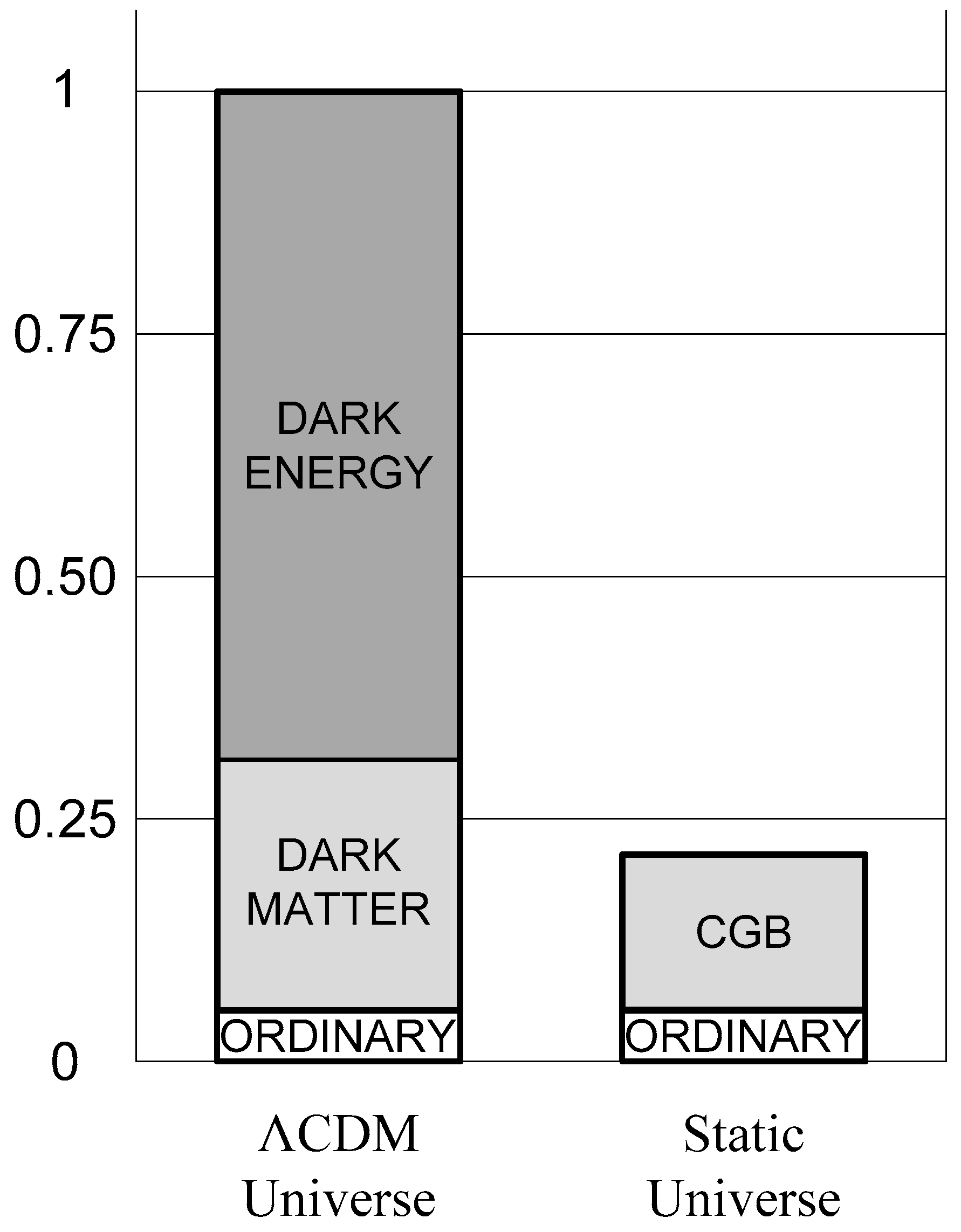
Figure 10.
Energy densities of the principal constituents of a universe and of a static universe with CGB, normalized to the critical energy density of a ΛCDM universe.
Figure 10.
Energy densities of the principal constituents of a universe and of a static universe with CGB, normalized to the critical energy density of a ΛCDM universe.
This estimate of in a static universe is consistent with estimates of in a ΛCDM universe. For example, from Planck 2018 measurements of CMB anisotropies, [57] infers energy densities of ordinary baryonic matter , dark matter , and dark energy .
Neither of the main constituents of a ΛCDM model universe, dark matter or dark energy, has been detected. Neither has the main constituent of a static model universe of this paper, a CGB, been detected. Yet both models predict essentially the same energy density of ordinary baryonic matter, about 5 percent of . A significant difference, however, is that the “base ΛCDM” model is “the standard spatially-flat 6-parameter ΛCDM cosmology having a power-law spectrum of adiabatic scalar perturbations” [57]. In contrast, the static model uses just one parameter, total energy density, to get the good fit of the distance modulus function to SN-Ia light-curve data in Fig. 9, and arrives at essentially the same estimate of ordinary baryonic energy density as the ΛCDM model. And even that one parameter, total energy density, is tightly constrained by Eq. (82).
3.13. Hubble constant, drag constant, dipole anisotropy, and cosmic gravitational background (CGB)
This section, supported by Apps. V, W, and X, summarizes some of the recent results of measurements of the Hubble constant, . This section relates these measurements to the scalar time-dilation drag constant , and to the temperature of the cosmic gravitational background (CGB), and to the energy density of the CGB, assuming the CGB is a collection of spin-1 bosons in thermal equilibrium obeying photon statistics.
Despite the meticulous collaborative efforts of large teams, a consensus on the value of has not yet been reached. The discrepancies in measurements, in some cases greater than five standard deviations, is referred to as the Hubble tension. Table 3 summarizes results of some of these collaborations.
In Table 3, the temperature of the CGB in a static, homogeneous universe is found from the Hubble constant by combining Eqs. (51) and (70) to get
(85)
The temperatures of the CGB in a static, homogeneous universe are given for each of the measured values of in the last column of Table 3.
The value of measured by the SH0ES Team, [60], and the inference of the Planck Collaboration CMB observations from the standard ΛCDM cosmological model, [57], despite their accuracies of the order of 1 percent or so, differ by more than five standard deviations.
In 1999, the Hubble Space Telescope Key Project team combined the results of several types of measurements of the Hubble constant at that time and concluded that they fell in the range of [58,59]. Since the more recent measurements in Table 3 still roughly fall in this same range and no resolution of the Hubble tension seems imminent at this time, this broad range of values of is used in this section.
If the CGB is a stochastic vector-field background, it might be expected to exhibit the same dipole anisotropy that the cosmic microwave background (CMB) does. That is, if the CGB is a collection of indistinguishable, massless, spin-1 bosons obeying photon statistics and is in thermal equilibrium at absolute temperature , and if the CGB is at rest with respect to the apparent rest frame of the CMB for the local group of galaxies [64,65], then the fractional temperature and frequency shifts of the CGB might be expected to be the same as the fractional temperature and frequency shifts of the CMB.
To lowest order in , the normalized speed of the Earth through the rest frame of the CMB, the observed temperature of the CMB with respect to the equilibrium temperature is [66] , and the apparent temperature shift is , where is the angle between the boson velocity and the velocity of the Earth through the CMB. The observed temperature is greatest in the direction toward which the Earth is moving.
The WMAP satellite experiment [67] found a maximum temperature increase of the CMB of in a direction near the Virgo cluster, which, for a CMB temperature of 2.725 K, corresponds to and a velocity of the solar system with respect to the CMB of 370 km/s. Taking into account the rotation of our galaxy gives a net velocity of the local group of galaxies [64,65] relative to the CMB of [66].
If the velocity of the solar system with respect to the CMB, 370 km/s, is the same with respect to the CGB, then the maximum temperature increase of the CGB would be times the equilibrium temperature of the CGB. Since the equilibrium temperature of the CGB in a static universe is about , as shown in Table 3, the maximum temperature increase of the CGB from the dipole anisotropy is about
(86)
If the CGB is responsible for the stochastic motion of particles, then experiments might someday be able to distinguish a secular drift of free particles with respect to the direction of the Virgo cluster, corresponding to this small dipole anisotropy in the equilibrium temperature of the CGB.
Since the root-mean-square gravitational field of the CGB is equal to the scalar time-dilation drag constant from Eq. (70), then
(87)
One result of this equality is that the Hubble constant is related to Planck’s constant, from the Stefan-Boltzmann law, Eqs. (44) and (50), by
(88)
One consequence of this relationship is that the CGB makes the classical limit, , unattainable.
Also from Eq. (50), Table 4 shows the mean energy density of the CGB in all frequencies depending on the value of the Hubble constant as
(89)
3.14. Quantum oscillators in the cosmic gravitational background (CGB)
If the cosmic gravitational background (CGB) is an ensemble of indistinguishable, massless, spin-1 bosons obeying photon statistics, then the stochastic dipole gravitational fields of the CGB will cause any bound or unbound particle to undergo stochastic motion, even in its lowest energy state. The behavior of quantum particle oscillators in the CGB, and specifically their mean energies and their effective diffusion coefficients, seems to be consistent in all respects with the behavior of particle oscillators obeying the Schrödinger wave equation. The suggestion that the CGB might be causally related to stochastic mechanics and the Schrödinger equation is supported by the calculations in App. Y.
The calculations in App. Y regarding the mean energy of quantum oscillators in the CGB closely follow the calculations in [49] of the generalized Nyquist relation and the fluctuation-dissipation theorem applied to stochastic electromagnetic fields. In [49], it is shown that the mean energy of a quantum oscillator depends only on the natural frequency of the oscillator and on the absolute temperature of the stochastic vector field in which the oscillator is immersed. The mean energy of an oscillator is independent of all other characteristics of the stochastic vector field other than its temperature.
In particular, the mean energy of an oscillator in a stochastic vector field is independent of the type of fluctuation force and radiative dissipation force, whether electromagnetic or gravitational, and independent of the power spectral density and mean energy density of the stochastic field, other than through its temperature. From the Stefan-Boltzmann law, the mean energy density of the cosmic microwave background (CMB), given in Eq. (52), depends only on the absolute temperature of the CMB, which is , as measured by the FIRAS instrument on the COBE satellite [51]. The mean energy density of a vector-field CGB in a static universe obeys the same Stefan-Boltzmann law, given in Eq. (50), but at an absolute temperature about , as estimated in Sec. 3.13.
Similarly, from Planck’s second quantum theory and the generalized Nyquist relation in [49], the mean energy at the absolute temperature of a one-dimensional oscillator at natural frequency ,
(90)
is independent of any of the characteristics of the stochastic vector field that causes this mean energy, other than its absolute temperature.
Figure 11 shows this dependence of mean oscillator energy on natural frequency of a one-dimensional oscillator immersed in the CGB. From Eq. (90), at high resonant frequencies , the mean energy of a 1-dimensional oscillator is , the zero-point energy of the oscillator. In a field theory of gravitation relating quantum fluctuations of the vacuum to the curvature of spacetime, Sakharov proposed that the zero-point energy has a cutoff at about the Planck energy, , which “determines the limit of applicability of present-day notions of space and causality” [2,68].
For free or weakly-bound particles or high temperatures (), the mean energy is . Since the absolute temperature of the CGB in a static universe is about , the mean energy in the CGB of a free or weakly-bound particle with one degree of freedom and with , from Eq. (90), is about .
If there is no CGB, and there is only a CMB, then since the absolute temperature of the CMB is , the mean energy in the CMB of a free or weakly-bound charged particle oscillator with , from Eq. (90), is . This energy corresponds to the kinetic energy of a proton moving at about 200 m/s, which is slower than sound in air at standard temperature and pressure.
In a combined CMB and CGB, the mean energy of a one-dimensional free or weakly-bound uncharged particle oscillator with , is about . Because , the effective absolute temperature of a combined CMB and CGB for a charged particle oscillator is little changed from and the mean oscillator energy is little changed from that shown in Figure 11.
Not only is the mean energy of a particle oscillator independent of all features of the stochastic vector field in which it is immersed, other than temperature, but so is the effective diffusion coefficient. Next, this section estimates the diffusion coefficient of particles immersed in the CGB, and shows that it is consistent with a causal relationship between the CGB and the Schrödinger wave equation.
To recap Sec. 3.6 and Apps. N and P, the displacement of a one-dimensional simple harmonic oscillator of mass , resonant angular frequency , and damping constant , driven by a dipole gravitational wave with constant amplitude and polarization in the direction, satisfies the equation of motion (N.1), and the solution of (N.1) is given by (N.2). The damping constant was found at (N.13) to be , which is also the line width , defined as the full width at half-maximum (FWHM) of the energy spectrum of the oscillator for .
The derivation of the properties of the CGB through Nyquist relations in App. P begins with consideration of a 1-dimensional simple harmonic oscillator of mass , amplitude , and resonant frequency immersed in the CGB, as in Eq. (P.1). The root-mean-square displacement of the oscillator is . The root-mean-square speed of the oscillator is . In terms of oscillator parameters, the zero-point energy of the oscillator immersed in the CGB is
(91)
Defining the diffusion coefficient of the oscillator as , and combining with Eq. (91) gives
(92)
According to [69], any particle of mass that is constantly undergoing a Brownian motion with diffusion coefficient obeys the Schrödinger wave equation.
An approximate derivation of the diffusion coefficient of an oscillator immersed in the CGB that involves somewhat less circular reasoning than the derivation of Eq. (92) is given in App. Y. Only the CGB dipole gravitational wave modes within about a line width about the resonant frequency contribute significantly to the resonant amplitude of the oscillator. As long as and the number of field modes of both polarizations within the frequency band is much greater than 1, then the field modes within the resonant frequency band about combine to produce effectively a single mode with an angular frequency about equal to and with an amplitude , where is the mean amplitude of each of the modes in the band [33]. Because this estimate neglects the contribution of CGB wave modes outside the narrow band , this approach in App. Y underestimates the diffusion coefficient as , a factor smaller than found in Eq. (92).
Further suggesting that the CGB has the same quantization as the cosmic microwave background (CMB), obeying photon statistics, comes from considering a particle at rest in a static universe. According to App. T, a particle at rest in a static universe will remain at rest in a zero-energy state until a specific force of at least is applied to it, where is the Hubble constant and is the dimensionless curvature constant defined at Eq. (59). Then it will be at least in the lowest energy state above zero. The wavenumber corresponding to that first excited state must be of order . That is, the wavelength of the first excited state is of the order of the length scale of the observable universe, . Then the frequency of the first excited state is of order , and its energy is of order
(93)
Lending support to these concepts and estimates, [70] found that a particle undergoing uniform acceleration satisfies a one-dimensional Schrö din ger equation with quantized energy levels at integers ,
(94)
so that the first excited state is , consistent with Eq. (93).
In summary, the internal motion of the universe appears to produce a cosmic gravitational background, a fluctuating gravitational vector field, everywhere. A cosmic background of dipole gravitational noise, similar to the cosmic microwave background, would produce a Brownian motion of all particles most noticeable for small particles. Any particle of mass that is constantly undergoing a Brownian motion with diffusion coefficient obeys the Schrödinger wave equation [69]. Appendices K, O, P, and Y suggest that an oscillator of mass immersed in the CGB does have a diffusion coefficient , thereby suggesting a causal relationship between the CGB and the stochastic mechanics underlying the Schrödinger equation.
4. Discussion
This section discusses some of the concepts that have been proposed in this paper. Some of the proposed concepts are well supported by multiple examples of benchmarking with known results and by self-consistency of the results derived in very different ways. This section attempts to point the way towards experiments and numerical analyses that can be performed, either now or in the future, to test these concepts.
The proposed concepts, roughly in the order presented in the paper, fall into these six categories:
- Gravitation, like electromagnetism, is fundamentally a vector field.
- Dipole gravitational waves exist and, like electromagnetic waves, apply forces to particles.
- Gravitational fields, like electromagnetic fields, are quantized and mediated by massless spin-1 bosons.
- A cosmic gravitational background (CGB), like the cosmic microwave background (CMB), is an ensemble of spin-1 bosons obeying photon statistics at an equilibrium temperature.
- A solution of the Einstein equation for a static, homogeneous universe, of which the CGB is the principal component, accounts for key cosmological observations, like: The Hubble redshift; the appearance of cosmic acceleration in SN-Ia light curves; and a density of ordinary baryonic matter that is only about 5 percent of the critical density of a lambda-cold-dark-matter (ΛCDM) universe.
- The CGB with its stochastic vector fields might be the “hidden variable” that underlies stochastic mechanics and the Schrödinger equation.
These six categories of proposed concepts are interrelated. In particular, the first four categories are closely interdependent. If the gravitational field is fundamentally a vector field, rather than a tensor field, then dipole gravitational waves do exist and do apply forces to all particles, the gravitational field is mediated by spin-1 gravitons rather than spin-2 gravitons, and gravitons do form a stochastic background governed by photon statistics.
Conversely, if the gravitational field is not a vector field, then dipole gravitational waves likely do not apply forces to particles or form a stochastic background in equilibrium with particles, and gravitons are spin-2 bosons, not spin-1.
From the inception of general relativity in 1915, the view has prevailed that the gravitational field must be a nonlinear tensor field, because a linearized treatment cannot account, as the tensor theory does, for the precession of planetary orbits. The alternative view explored in this paper is that gravitation is fundamentally a vector field and that the gravitation of the energy density of fields is a nonlinear correction to the gravitation of masses, a correction needed, for example, to calculate the precession of planetary orbits.
Fortunately, the means to determine whether the gravitational field is fundamentally a vector field or a tensor field have now become available with the advent of gravitational wave astronomy and the observations of mergers of compact binaries. As was discussed in Sec. 3.4, and is discussed in Sec. 4.1 to follow, this determination should be relatively straightforward by an analysis of low-frequency strain data that has already been compiled from observations of many dozens of compact-binary mergers. Either the low-frequency strain data will reveal the existence of low-amplitude dipole gravitational waveforms at the orbital frequency of merging binaries in accordance with the strong-field nonlinearities that produced them in the source region, or the data will not.
4.1. Gravitation as a vector field
Section 2, “Method,” showed that in the linear approximation of general relativity, the field and force equations can be transformed into vector equations with forms identical to the covariant Maxwell and Lorentz force equations. These transformations support the concept that gravitation could be a vector field, as do the handful of examples of benchmarking of the linearized results with the fully nonlinear strong-field theory that were itemized in Sec. 1, “Introduction,” and discussed in this paper.
The historical reason why general relativity was developed first as a fully nonlinear tensor theory of gravitation, rather than as a vector theory, was briefly discussed in Sec. 1. In the years before 1915, when Einstein was developing his theory of general relativity, only one astronomical observation was available for him to benchmark his incipient theory. That was the precession of the perihelion of Mercury’s orbit. When Einstein found his theory to be consistent with the 1859 observation [71] of French mathematician and astronomer, Urbain Le Verrier, of a 45 arcsecond/century advance of Mercury’s perihelion (now more accurately known as 43 arcsecond/century), that was the “confirmation” Einstein had been seeking.
In 1915, Einstein wrote, “... I find an important confirmation in this most radical theory of relativity: it turns out that it explains qualitatively and quantitatively the secular precession of the orbit of Mercury in the direction of the orbital motion, as discovered by Leverrier, which amounts to about 45” per century ...” [72; translated in 2].
Once the equations were benchmarked to Mercury’s precession and published on November 25, 1915 [72], from a session on that date [2], Einstein published his final formulation of the field equations one week later, on December 2, 1915, declaring, “With this step, general relativity is finally completed as a logical structure” [73; translated in 2].
The reason that the precession of Mercury’s orbit was such a compelling confirmation for Einstein, is that this result could not be obtained from the linearized theory alone. The linearized equation of motion is only valid for weak gravitational potentials, , of a source mass , much less than the specific kinetic energy of a test mass, . For bound planetary orbits, the potential of the Sun, , is comparable to the specific kinetic energies of the planets, the condition is not satisfied, and the linearized equation of motion is unable to predict the orbital precession that Einstein’s exact nonlinear theory could predict correctly. That means a vector theory of gravitation, which neglects the gravitation of gravitational fields, is insufficient to explain the rate of precession of Mercury’s orbit.
Most of the key tests of general relativity since then, however, could be explained by the linearized theory, that is, a vector theory of gravitation that neglects the gravitation of fields. Section 3.2 showed that even the gravitational radiation from a well-behaved binary can be explained by a vector theory of gravitation.
To amplify this historical theme further, Table 6 recounts some of the key experimental and astronomical observations that have been used to test and guide the development of general relativity from its inception in 1915. Within a few years of Einstein’s publication of the tensor field equations, Eddington led an expedition that measured the deflection of starlight around the limb of the Sun [74]. This first test of general relativity only tested deflection of light in the linear approximation. That is, the test was of Eq. (16), the gravitational impulse delivered by, or to, a particle in uniform motion in the limit of small deflections, and Eq. (16) was derived from a vector-field formulation of general relativity.
The next key test of general relativity highlighted in Table 6, the measurement by Pound and Rebka [53] of the gravitational frequency shift of light in the gravitational potential of Earth, did not even require a vector-field formulation of general relativity to account for the results. In these measurements, a Newtonian scalar potential accounted for the energy and frequency change of light in the gravitational potential of Earth.
The discovery of binary pulsars with the Arecibo radio telescope in 1974 was published in 1975 by Hulse and Taylor [40]. Following many years of data compilation, Taylor and Weisberg showed [41] that the decay of the orbit of the binary pulsar, PSR 1913+16, was consistent with the predictions of general relativity for production of gravitational radiation by a rotating mass quadrupole. This was the first indirect evidence for the existence of gravitational waves, and appeared to be a confirmation of the quadrupole nature of gravitational waves from a tensor theory of gravitation. As shown in Sec. 3.2, however, if the radiation from PSR 1913+16 comprises a linear superposition of interfering dipole gravitational waves from the pulsar and its companion, rather than quadrupole waves from the binary, the observed orbital decay would be identical.
Section 3.2 and App. H show that even the gravitational radiation from a gravitationally bound binary can be fully explained by a vector theory of gravitation, as indicated in Table 6. The nonlinear tensor field equations of general relativity are not needed. A superposition of linearized dipole gravitational waves from each of the masses of a rotating binary can account fully for the gravitational waves and gravitational radiation from a binary. Dipole gravitational waves from each of the masses interfere with each other to produce the appearance of quadrupole radiation.
The acceleration field of Eq. (11) predicts gravitational dipole radiation from a nonrelativistic binary that is identical in all respects to conventional quadrupole radiation, except that the gravitational dipole radiation accelerates particles, just as electromagnetic radiation accelerates charged particles, and the quadrupole radiation only produces ripples in the coordinates of spacetime. That is, dipole radiation from rotating binaries applies forces to particles in accordance with Eq. (24), and quadrupole radiation does not. The strain signal at a gravitational wave detector, however, is the same.
The angular distribution and total power of dipole radiation from a rotating binary in the vector theory are identical to the angular distribution and total power of quadrupole radiation in the tensor theory. The acceleration field of Eq. (11) in the transverse gauge shows that the superposition of dipole gravitational waves in the radiation zone from each of the masses of a binary has exactly the same perturbation metric, Eq. (18), exactly the same angular power distribution, Eq. (19), and exactly the same total power, Eq. (20), as the quadrupole radiation. That is, Sec. 3.2 shows that the quadrupole radiation from a rotating binary is just the superposition of dipole waves from each of the masses.
Strong fields in the source region of merging compact binaries disrupt the interference of dipole waves from each of the masses. This disruption should allow dipole waves to be detected in the strain signals of gravitational wave observatories. An estimate of the magnitude of the dipole wave signals that might be expected from the merger event GW 150914 was given by the strain waveform model in Sec. 3.4.
In well-behaved binaries, like the binary pulsars that were first discovered in the 1970s [40,41,42], the dipole gravitational waves of each member of the binary nearly completely interfere, leaving only radiation characteristic of quadrupole waves. In a merging compact binary, on the other hand, the interference of the dipole gravitational waves of each member is disrupted by the strong nonlinear fields in the source region. In such cases, the strain signals measured at gravitational wave observatories, like LIGO [36,37], would reveal the existence of dipole gravitational waveforms at the orbital frequency. As discussed in Sec. 3.4, such low-frequency strain signals may already have been detected at amplitudes of the order of 10 percent and power levels of the order of 1 percent of the quadrupole signals.
In a metric theory of gravitation, Shapiro time delay [45] and deviation of radiation [46] by strong gravitational fields affect gravitational radiation just as they do electromagnetic radiation. Analysis of the strong fields and gross distortions of spacetime in the source region of coalescing compact binaries certainly requires the full nonlinear tensor theory of general relativity. These strong nonlinear effects can disrupt the otherwise nearly complete interference of dipole waves resulting from the gradual decay of a well-behaved binary. It is this nonlinear disruption of interference of dipole waves from each member of a coalescing compact binary that has possibly already been detected by gravitational wave observatories at the orbital frequency of the binary at the low-frequency end of the strain-wave spectrum. The waveform model of Sec. 3.4 suggests that in the merger event, GW150914, at least about 0.5 percent of the gravitational wave power was radiated as dipole gravitational waves at the orbital frequency. To the extent that the dipole gravitational radiation was not in phase with the quadrupole radiation, the dipole radiation power might have been greater than this estimate.
The existence of strain waveforms at the orbital frequency is not dispositive unless the waveforms are directly related to the disruption of interference of dipole waves from each member of the binary. What would be dispositive of the existence of vector gravitational fields is a direct and unambiguous observation of the relation between the dipole signals at the orbital frequency and the nonlinear fields in the source region that produced them.
Drawing such a direct relation between dipole signals and nonlinear fields in the source region requires numerical relativity, but does not necessarily require a substantial overhaul of existing codes. The dipole fields that emerge from the source region can be treated as a linearized perturbation to the radiated fields, and the dipole fields can be calculated by piggy-backing subroutines on the existing codes of numerical relativity. Such calculations benchmarking the production of dipole gravitational waves to the strong-field source-region effects that disrupted their interference would be a dispositive confirmation of their existence.
If these numerical relativity calculations do benchmark, and do not falsify, the existence of dipole gravitational waves, then the potential payoff to gravitational wave observations is enormous. The same linearized, piggy-backed subroutines that benchmark the existence of dipole gravitational waves can then be used to characterize more accurately the parameters of every observed merger event.
Currently, the characterization of merger-event parameters is crude. For example, it took years of observations before the highly asymmetric merger event of 2019 could even exclude the possibility that all binaries in merger events had a mass ratio of one [48]. The strong-field effects that disrupt dipole-wave interference can provide an independent set of equations relating the parameters of merger events to allow them to be characterized more accurately.
This section has thus far discussed benchmarking of the acceleration field of Eq. (11), the radiation-zone field that falls off as and depends linearly on acceleration. The velocity field of Eq. (11), the source-region and near-zone field that falls off as , and is independent of acceleration, is also benchmarked in this paper.
Standing on much more well-established ground than the yet-to-be-tested existence of dipole waves in the radiation zone are the calculations in Sec. 2.2, and specifically Eq. (11), of the gravitational velocity field in the source-region and near-zone of a particle in arbitrary relativistic motion. As mentioned in Sec. 2.2, the velocity field in Eq. (11) has already been benchmarked to the well-known strong-field cases of: Hilbert repulsion [16], a spherical mass in uniform motion [14,15], and unbound orbits in a strong field [13,21].
Hilbert found that a particle moving radially at speeds above , in the static (Schwarzschild) field of a central mass appears to a distant observer to be repelled by the central mass [16]. Hilbert’s result applies even to strong gravitational fields, but only for radial motion of the particle. Equation (11) generalizes Hilbert’s result to particle motion in all directions, not just radial, and is benchmarked in the weak-field limit to Hilbert’s result for radial motion in a strong field.
Similarly, the exact dynamic field of a spherical mass in uniform motion, calculated from an exact metric first derived in [14], was shown through a coordinate transformation [15] to be identical in the weak-field limit to Eq. (11). And the exact unbound orbit of a particle in a strong central field, calculated by Chandrasekhar in [13], was shown in [21] to correspond to the Lorentz-transformed unbound orbit of the particle in the weak field of the central mass in uniform motion predicted by Eq. (11).
Just like the capability to confirm the existence of dipole gravitational waves, the capability to confirm the existence of the repulsive gravitational fields predicted by Hilbert in [16] is available today. As detailed in [15,24] and outlined in Sec. 2.2, an experimental test of Eq. (11) at ultrarelativistic speeds can be performed on a tabletop at any location next to the 27-km-circumference beamline of the Large Hadron Collider (LHC) without interfering in any way with the normal operations of the LHC.
This first detection of repulsive gravity at the LHC would be a dramatic demonstration of the utility of the vector-field formulation of linearized general relativity in Eq. (11). But this test would not exercise the full power of Eq. (11). Each proton bunch would only deliver its repulsive impulse to the detector for the brief moment that it is moving radially towards the detector within an angle of order mrad [15]. The full power of Eq. (11) for calculating gravitational fields for all impact parameters at all particle speeds would not be demonstrated.
Also detailed in [15,24] and outlined in Sec. 2.2 is a test of the gravitational fields predicted by Eq. (11) for non-radial motion at speeds up to the order of sound speeds in solids. Again, the capability is available today. A test of the gravitational fields predicted by Eq. (11) can be performed on an existing flywheel, such as the NASA G2 Flywheel Module [25] with a modified rotor [15,24].
Section 3.1 presented an additional benchmarking of the velocity field in Eq. (11). That section calculated the transverse gravitational impulse, in the weak impulse approximation, delivered to a test mass by a particle in uniform motion at any speed, up to and including the speed of light. The angular deflection in a weak field calculated from the linearized vector theory in Eq. (16) is benchmarked against the deflection of light, such as in [74], and against the known deflection of nonrelativistic particles.
4.2. A cosmic gravitational background
Section 2.1 demonstrated that the field and force equations of general relativity in the linear approximation can be transformed into equations that are identical in form to the Maxwell field and Lorentz force equations. This parallel opens the possibility that gravitation is fundamentally a vector field, just like electromagnetism, and that the tensor fields of general relativity just include corrections to the vector theory that account for the gravitation of fields in addition to masses. If that is the case, then weak-field gravitation theory can be developed in close analogy to electromagnetism theory, as was suggested by Table 1 in Sec. 1, “Introduction.” One of the analogies that was explored in this paper is that of a cosmic gravitational background (CGB) in close analogy to the cosmic microwave background (CMB).
The electromagnetic field is a vector field that causes charged particles to accelerate. Accelerating charges produce electromagnetic radiation, and electromagnetic radiation accelerates charges. Electromagnetic fields are mediated by spin-1 bosons governed by photon statistics. The stochastic electromagnetic fields that fill the universe, known as the CMB, are in equilibrium with the charged particles in the universe at an equilibrium temperature of about 2.7 K.
This paper explores the possibility that the gravitational field is fundamentally a vector field that causes masses to accelerate in the radiation zone in accordance with Eq. (24), and that causes nonrelativistic accelerating masses to produce gravitational radiation in accordance with Eq. (31). If the gravitational field is a vector field, then gravitational fields are mediated by spin-1 bosons governed by photon statistics. Then the stochastic gravitational fields that fill the universe, herein called the cosmic gravitational background (CGB), are in equilibrium with particle masses in the universe at an equilibrium temperature estimated in Sec. 3.13 to be about 20 to 22 K.
If there are spin-1 gravitons that do obey photon statistics, then the properties of the CGB are determined solely by the equilibrium temperature of the CGB. For example, the mean total energy density of the CGB is given by the Stefan-Boltzmann law, Eq. (44). Just as the mean-square electromagnetic fields of the CMB are proportional to the energy density of the CMB, the mean-square fluctuating gravitational field of the CGB, , is proportional to the mean energy density of the CGB, , as shown in Eq. (50). And the root-mean-square fluctuating gravitational field of the CGB, , is then given in terms of the equilibrium temperature by Eq. (51).
Section 3.13 and Table 4 showed that in a static, homogeneous universe comprising a CGB and ordinary matter, the energy density of the CGB must be about 900 200 , and its equilibrium temperature, therefore, must be about 211 K. In Sec. 3.11 and Fig. 9, the fit of the distance modulus function to Supernova Type Ia (SN-Ia) light-curve data supports these estimates in a static, homogeneous universe.
The equilibrium temperature of the CMB was measured by the FIRAS instrument on the COBE satellite to high accuracy as TCMB = 2.725 ± 0.002 K [51]. And the maximum temperature increase from the dipole anisotropy of the CMB was measured by the WMAP satellite experiment as [67], with a remarkable accuracy of . By contrast, the equilibrium temperature of a CGB, if it exists, has not been measured at all.
There are several potential observables of a CGB, from which its equilibrium temperature and root-mean-square gravitational field, , may be ascertained, including:
- The excitations of molecular states in the CGB;
- The drag deceleration of particles moving through the CGB;
- The dipole temperature anisotropy of the CGB;
- The minimum mean energy of a weakly bound quantum oscillator.
Appendices N and P calculate the behavior of a resonant oscillator in a stochastic gravitational field like the CGB. The Nyquist relations essentially state that only those gravitational field modes having a frequency within about the linewidth of the resonant frequency of the oscillator contribute significantly to the resonant amplitude of the oscillator. Given a Planck distribution of spin-1 gravitons from Eq. (41) and a measured amplitude of a resonant oscillator, therefore, an equilibrium temperature of the CGB can be inferred.
A historical review of the CMB [75] noted that the first evidence of a 3-K CMB was observed as early as 1940 [76,77], decades before the 1965 discovery by Penzias and Wilson [78] was recognized as such. McKellar [76] and Adams [77] observed excited rotation states of cyanogen (CN) molecules in interstellar space, corresponding to a sky temperature of 3 K. In particular, “should the 3874.6 interstellar line actually be the line of the 0,0 violet CN band” and “if is not more than one-third …as intense as , the maximum “effective” temperature of interstellar space would be 2.7 K …” [76]. More than half a century passed, however, before the observation of excited rotation states in CN molecules in interstellar space was related to the 3-K temperature of the CMB [79].
The same approach, using excitations of molecular states in the CGB and line intensity ratios, might also be used to observe a CGB with an equilibrium temperature of about 21 K.
Another potential observable of the CGB is the drag deceleration of particles moving through the CGB. Section 3.11 and Eq. (70) showed that the deceleration experienced by a nonrelativistic particle moving through the CGB in a flat spacetime is a constant equal to the root-mean-square gravitational field of the CGB, .
As discussed in Sec. 3.13, our solar system seems to have a speed with respect to the mean Hubble flow, that is, the rest frame of the CMB [64,65], of about [66]. It is reasonable to suppose that the rest frame of the CMB in our local group of galaxies would also be the rest frame of a CGB. In that case, any particles with relative speeds much less than a few hundred km/s would be affected about equally by the drag deceleration of the CGB.
For example, the Pioneer 10 and Pioneer 11 spacecraft are moving away from our Sun at speeds of about [80]. Since their relative speeds are much less than the speed of our solar system through the CGB, the Sun and both Pioneer spacecraft would be expected to be affected about equally by the CGB. Although CGB drag might therefore not be expected to play a role in the Pioneer anomaly [80,81], the time-dilation drag deceleration, , derived in Sec. 3.11, might be relevant in helping to understand this anomaly [33].
The speeds of particles in the outer regions of spiral galaxies, which can be hundreds of km/s, are a different matter. The effects of CGB drag on orbital dynamics of particles and the expected effects on galactic rotation curves and on the Tully-Fisher relation are calculated in [33]. The flattening of galactic rotation curves is generally attributed to dark matter [82,83] or to modified Newtonian dynamics [84,85], but can be modeled quite well based on the constant drag deceleration discussed in [33] and in Sec. 3.11.
Another potential observable of the CGB is the dipole temperature anisotropy discussed in Sec. 3.13 and estimated in Eq. (86). If the velocity of our solar system relative to the CMB, [66], is the same for the CGB, and if the temperature of the CGB, as shown in Table 3, is about 20 to 22 K, then the maximum temperature increase of the CGB from the dipole anisotropy is about 25 to 27 mK, as shown in Eq. (86). Thus, measuring the dipole temperature anisotropy of the CGB requires about 1,000 times greater accuracy than measuring the temperature itself. It may be that this accuracy can be achieved using line intensity ratios of excited molecular states in the CGB. Or it may be that other techniques are needed to achieve the required precision of temperature measurement.
If a CGB does exist at an absolute temperature of about 21 K, then according to Eq. (90) and Fig. 11, the minimum mean energy of a one-dimensional charged or uncharged particle oscillator is about 1.8 meV. If a CGB does not exist, and the only stochastic vector field is the CMB at an absolute temperature of about 2.7 K, then according to Eq. (90), the minimum mean energy of a one-dimensional charged oscillator is about 0.23 meV. A potential observable of the CGB, therefore, might be a minimum mean energy of particle oscillators much higher than 0.23 meV.
4.3. A static, homogeneous universe
Entwined with the concept of the CGB is the cosmological spacetime model that establishes the framework for the CGB. A simple and featureless cosmological spacetime model isolates the effects of the CGB independently of extraneous parameters.
The simplest and most featureless nontrivial cosmological spacetime is the static, homogeneous universe. Just as the Schwarzschild solution of Einstein’s equation has only one parameter, the central mass, the solution of Einstein’s equation for a static, homogeneous universe has only one parameter, total energy density. That is one reason why Schwarzschild chose a central spherical mass to be the first exact solution in 1916 [86,87], and that is one reason why Einstein chose a static universe to be the first exact cosmological spacetime model in 1917 [88,89].
The exact solution of Einstein’s equation for a static universe is parametrized in terms of total energy density . By the relationships in Eqs. (60) and (R.10) among the energy density, the curvature , and the cosmological constant , the solution can also be parametrized in terms of and .
The exact solution of Einstein’s equation for a static universe in Sec. 3.9 and App. R differs from Einstein’s exact solution in [88,89] in the choice of coordinates. A static, homogeneous universe has both rotational symmetry and translational symmetry. The most appropriate coordinates for the static cosmological spacetime model, therefore, are Cartesian coordinates, which take best advantage of the rotational and translational symmetries.
In spherical coordinates, the Laplacian operator, , of Einstein’s equation, Eq. (R.9), introduces a spurious singularity at the origin. The singularity at the origin was useful for Schwarzschild’s solution for a point mass in [86], but detracts from the generality of the solution for a homogeneous universe. The reason Einstein chose spherical coordinates, rather than Cartesian coordinates, for his spacetime model of a static universe may be that he could more easily benchmark his exact solution against Schwarzschild’s. That is, he might have chosen spherical coordinates despite the disadvantages for the same practical reason he chose to develop general relativity first as a nonlinear tensor theory, rather than as a linear vector theory: A means existed for benchmarking his results.
The standard metric forms of the Friedmann-Lemaître-Robertson-Walker spacetimes [90,91] are also most commonly expressed in spherical coordinates. These metric forms put the spacetime curvature in the space coordinates and not in the time coordinate. In a static, homogeneous spacetime, particularly one parametrized in Cartesian coordinates, curvature in the space coordinates is an unnecessary complication. The simplest and most appropriate spacetime coordinates for a static universe are Cartesian coordinates parametrizing a flat 3-volume and a time-dilation function parametrizing the time coordinate.
The most general coordinate parametrization of a static universe in Cartesian coordinates was first derived in [33], as was the special case of a flat 3-volume with a time-dilation function. As shown in Fig. 5 in Sec. 3.9, the metric component in Cartesian coordi nates has a discontinuity in slope at the origin. This difficulty is circumvented by the mathematical sleight-of-hand of solving Einstein’s equation only along a ray from the origin, and not along an infinite line through the origin. Then the Laplacian operator of the equation in Cartesian coordinates along the ray, , does not involve any spurious singularities or discontinuities at the origin. With the boundary conditions of at the origin and at , the metric of a static universe then takes the simple form of Eq. (59).
This simple exact solution of Einstein’s equation for a static, homogeneous universe, Eq. (59), using Cartesian coordinates for a flat 3-volume with a time-dilation function for the component of the metric, yields intriguing results when coupled with the concept of a CGB. A 1-parameter cosmological model of a static universe that comprises just two principal constituents, ordinary matter and a CGB, can account for the three principal cosmological observations underlying other far more complex models, like the “base ΛCDM” [57] model.
As noted in the Introduction in Sec. 1, the model of a static universe with CGB accounts for the three principal cosmological observations: The Hubble redshift in a static universe (in Sec. 3.10 and App. S); the appearance of cosmic acceleration in SN-Ia light curves in a static universe (in Sec. 3.12 and App. U); and a baryonic matter density of the order of 5 percent of the ΛCDM critical density in a static universe (in Sec. 3.12 and App. U).
The cosmological model of a static universe has an advantage over many other models that also account for the three principal cosmological observations. The correspondences of the model with observations are organic outgrowths of the exact metric itself. The Hubble redshift and the apparent cosmic acceleration of the universe are built-in features of the component of the exact metric with just one parameter. The baryonic matter density of the order of 5 percent of the ΛCDM critical density follows ineluctably from supposing the static universe principally comprises ordinary matter and a CGB.
Other models of the universe do offer correspondences with other cosmological observations besides the principal three. But these additional correspondences generally involve more arbitrary parameters, and are therefore of uncertain value.
When Freeman Dyson showed Enrico Fermi a 4-parameter meson particle model that gave good agreement between calculations and measurements, Fermi was not impressed, saying [92], “I remember my friend Johnny von Neumann used to say, with four parameters I can fit an elephant, and with five I can make him wiggle his trunk.” The ΛCDM/dark-matter/dark-energy “base ΛCDM” standard model is a 3-constituent, 6-parameter model of which two constituents, dark matter and dark energy, after decades of searching, have not yet been directly detected [57]. The static/CGB model is a 2-constituent, 1-parameter model of which one constituent, the CGB, has not yet been directly detected.
Though dark matter and dark energy have not yet been detected directly, there is much circumstantial evidence for their existence. By the same token, it might be argued that the existence of a CGB is also supported by circumstantial evidence. As shown in Sec. 3.14, the stochastic CGB might be what accounts for stochastic mechanics and the Schrödinger equation. As will be discussed in Sec. 4.4, every manifestation of quantum mechanical phenomena, like the uncertainty principle or the resonant behavior of bound quantum oscillators, might be considered a detection of the CGB.
Recent research does seem to support the possibility that our universe might actually be the static, homogeneous universe first proposed by Einstein in 1917 [88,89]. For example, the concept of “tired light,” first proposed by Zwicky in 1929 [93], has received renewed interest and support following recent measurements reported in [94].
The tired-light concept was considered an alternative to a model of an expanding universe that might explain the linear relationship discovered by Hubble of redshift with distance. Zwicky proposed that light might lose energy over time through collisions with particles in such a way that the Hubble redshift could be explained even in a static universe. Many other tired-light conjectures have been proposed since then, but none has yet been found to be compatible with all the observational evidence.
At a minimum, a viable tired-light hypothesis must satisfy the following conditions:
- Explain not just the linear relationship of apparent velocity with distance, but also the apparent cosmic acceleration measured in SN-Ia light-curve data;
- Explain the time dilation of distant cosmological events in accordance with the same velocity relationships;
- Give the same redshift factor for all wavelengths;
- Not cause blurring of images that would occur, for example, with a photon-scattering mechanism for the redshift.
The exact metric of a static, homogeneous universe, Eq. (59), derived in App. R, satisfies all these conditions. As shown in Secs. 3.10 and 3.12, the component of the metric itself explains the time dilation and apparent cosmic velocity and acceleration of distant cosmological events in all wavelength bands. No additional physical mechanism for tired light needs to be invoked. According to this exact solution of Einstein’s equation, light “gets tired” all by itself as a consequence of the curvature of spacetime in a static universe.
Section 3.10 noted that a pulse of light propagating through a static universe delivers a transverse momentum impulse to all the mass in its past light cone in accordance with the vector-field calculations in Sec. 3.1, and specifically with the well-known Eq. (16). A simple estimate of the energy loss by this mechanism shows that it accounts for the order of magnitude of the Hubble redshift in a static universe [33].
This order-of magnitude estimate of energy lost by the transverse impulse delivered by a pulse of light to the mass in its past light cone suggests that there might be a fundamental connection between the spacetime metric and the energy that is lost to the mass in the universe through this gravitational means. If so, then it would be interesting to inquire how the parameters of the ΛCDM model might need to be modified to account for this energy-loss mechanism in the calculation of total redshift. A good starting point for this inquiry would be an exact solution of Einstein’s equation in isotropic Cartesian coordinates with a time-dependent scale function for expansion and a time-dependent function for the metric component that accounts for both spatial expansion with time and time dilation with distance. In the limit of no expansion, that is, a static universe, the metric should approach that of Eq. (59).
The “first direct empirical reproducible observation” of tired light may have been reported recently in [94]. Datasets from three telescopes and observations of more than 30,000 galaxies shows evidence that the redshift of galaxies depends on their rotational direction relative to the rotational velocity of the Milky Way. If this small bias in redshift is also observed at large cosmological distances, for , that would suggest that light loses energy as it travels, and not as a result of an expanding universe [94].
Other recent observations also support the possibility that we live in a static, homogeneous universe. The composition of a static, homogeneous universe should look about the same at every distance and in every direction. In an expanding universe, by contrast, the “early universe” at high would be expected to have a greater population of young galaxies and a smaller population of mature galaxies than the universe does locally. Predictions for what the deep galaxy surveys of the James Webb Space Telescope (JWST) would find were made in 2018 [95].
Even before JWST was launched at the end of 2021, the existence of massive, mature galaxies at high redshifts was reported [96]. And since then, other research groups have reported similar findings of massive mature galaxies at redshifts as high as [97,98,99]. These observations of mature galaxies in the “early universe” at high have not yet been explained within the “base ΛCDM” standard model. But they are consistent with a model of a static, homogeneous universe.
Direct measurements can be done that will resolve the question of whether our universe is accelerating or not. One such experiment was proposed in [100], based on measuring the Sandage-Loeb [101,102] drift in the redshift of the hydrogen absorption line at 21 cm in hundreds of thousands of dense hydrogen clouds. Over the course of a decade or so, the slight increase in the redshift of the 21-cm line that would indicate acceleration of the order of 11 mm/s/yr should be observable, and the cosmic acceleration should be measurable by that means. If the universe is not accelerating, that null result should also be observable by that means.
If a direct measurement of cosmic acceleration does turn up a null result, it should not be a great surprise. A maximum-likelihood analysis of the Joint Lightcurve Analysis catalogue [103] of 740 spectroscopically confirmed Type Ia supernovas with high-quality light curves found “marginal evidence,” less than or about , for the claim that the universe is accelerating [104]. The analysis in [104] is “quite consistent with a con stant rate of expansion,” that is, no acceleration.
No matter how well the distance modulus function may fit the SN-Ia light-curve data for an accelerating universe, however, the distance modulus function does not directly measure cosmic acceleration. It only measures the appearance of cosmic acceleration. As shown in Secs. 3.10 and 3.12 and App. S, even a static universe gives the appearance of cosmic acceleration. In particular, Eq. (66) shows that time dilation and the redshift parameter increase faster than linearly with distance in a static universe, at a rate that depends only on energy density. Thus, the appearance of cosmic acceleration in SN-Ia light curves does not mean that the universe is accelerating or even that the universe is expanding at all. The only way to tell whether the universe is accelerating or not is by a direct measurement of acceleration, such as by the means proposed in [100].
Whether the universe is static or expanding, evidence suggests that a preferred rest frame exists, one that is at rest with respect to the mean Hubble flow. The evidence is in the form a dipole anisotropy in the temperature of the CMB. As discussed in Sec. 3.13 and App. W, the temperature anisotropy suggests that the Earth is moving at a speed of 370 km/s with respect to the rest frame of the CMB. Whether this rest frame corresponds to the mean Hubble flow for our local group of galaxies or globally to a static universe, one thing is certain. The first postulate of the special theory of relativity is not strictly applicable, at least within our local group of galaxies.
According to the first postulate [105], if a system of coordinates is chosen so that, in relation to it, physical laws hold good in their simplest form, the same laws hold good in relation to any other system of coordinates moving in uniform translation relatively to . Physical laws hold good in their simplest form in the rest frame of the CMB. The same laws do not hold good in relation to any other system of coordinates moving in uniform translation relatively to the rest frame of the CMB. In particular, in any other system of coordinates moving in uniform translation, free particles are accelerated.
There is no reason to believe that the rest frame of the CMB should not also be the rest frame of a CGB. In fact, at thousands of times higher energy density than the CMB, the CGB should carry along the CMB. For this reason, one expects the same fractional temperature anisotropy, as discussed in Sec. 3.13 and App. W.
A static, homogeneous universe with a CGB has narrow bounds of possible energy densities. The exact solution of Einstein’s equation for a static universe puts an upper bound on the energy density. As shown in Eq. (78) and Fig. 8, a static solution of Einstein’s equation is not supported for energy densities greater than , where is the critical energy density of a ΛCDM universe. The existence of a CGB with a root-mean-square gravitational field equal to the time-dilation drag constant, as found in Eq. (70), implies through the Stefan-Boltzmann law, Eq. (50), that the CGB has an energy density equal to . Therefore, in a static universe with two principal constituents, ordinary matter and a CGB, the maximum possible energy density of ordinary matter is .
But if one requires a good fit of the distance modulus function of SN-Ia with energy density (or curvature ), in Fig. 9 for example, one finds that there is a minimum bound on the energy density of ordinary matter in a static universe as well, such that the total energy density of a 2-constituent, static universe is between and , as shown in Eq. (82). Because the energy density of the CGB is , the energy density of ordinary matter in a 2-constituent, static universe must be between and , as indicated in Eq. (84). And that is how a 2-constituent, 1-parameter model of a static universe arrives at the same estimate for energy density of ordinary matter as the 3-constituent, 6-parameter “base-ΛCDM” model.
In addition to the correspondences with redshift, cosmic acceleration, energy density of ordinary matter, and existence of mature galaxies at high , this model of a 2-constituent static universe relates the Hubble constant to the quantum mechanical Planck’s constant through the equilibrium temperature of the CGB in Eq. (88). Planck’s constant is known to high precision. As shown in Table 3 in Sec. 3.13, recent measurements of the Hubble constant are spread over a range of 10 percent or more. The uncertainty in the Hubble constant results in an uncertainty in the temperature of the CGB, , of about 5 percent. When a reliable and accurate determination of the Hubble constant is made, the temperature of the CGB can be accurately determined. It is not inconceivable, however, that an accurate determination of the temperature of the CGB might instead lead to the first reliably accurate determination of the Hubble constant.
The concept of a cosmic background endowing all of space with physical qualities can claim the endorsement of the founder of general relativity, who calls the idea of space without physical qualities “unthinkable”:
“There is a weighty argument to be adduced in favour of the aether hypothesis. To deny the aether is ultimately to assume that empty space has no physical qualities whatever. The fundamental facts of mechanics do not harmonize with this view ... according to the general theory of relativity space is endowed with physical qualities; in this sense, therefore, there exists an aether. According to the general theory of relativity space without aether is unthinkable; for in such space there not only would be no propagation of light, but also no possibility of existence for standards of space and time (measuring-rods and clocks), nor therefore any space-time intervals in the physical sense.” [106]
4.4. Stochastic mechanics
If gravitation is fundamentally a vector field like electromagnetism, which is a possibility discussed in the Introduction and in Sec. 4.1, then it seems likely, if not necessary, that the gravitational field, like the electromagnetic field, would be quantized as spin-1 bosons obeying photon statistics and that the temperature dependence of the mode density of the cosmic gravitational background (CGB), Eqs. (41) and (42), would be identical to that of the cosmic microwave background (CMB).
A CGB of stochastic dipole gravitational waves, quantized as spin-1 bosons obeying photon statistics, seems to possess the properties necessary to provide a causal basis for stochastic mechanics and the phenomena described by the Schrödinger wave equation.
Unlike quadrupole gravitational waves, dipole gravitational waves in the radiation zone push and pull on particles in accordance with the equation of motion, Eq. (24). The stochastic nature of the CGB means that the motion of particles in response to the fields appears to be random even though the motion is causally related to the fields that produce it.
A cosmic background of dipole gravitational noise, similar to the CMB, would produce a Brownian motion of all particles most noticeable for small particles. Unlike particles in the CMB, all particles, charged and uncharged, would respond the same to the stochastic forces of the CGB.
Nelson [69] demonstrated in 1966 that the Schrödinger equation could be derived entirely classically if there exists a physical mechanism that subjects every particle of mass to a Brownian motion with diffusion coefficient and no friction. This paper proposes that a cosmic background of dipole gravitational radiation might be such a mechanism.
Bohm [107] proposed an early deterministic, or causal, interpretation of quantum mechanics in terms of non-local “hidden variables, which in principle determine the precise behavior of an individual system, but which are in practice averaged over in measurements ... .” Like the probabilities of statistical mechanics, the probabilities of quantum mechanics “are regarded as only a practical necessity and not as a manifestation of an inherent lack of complete determination ... .” A companion paper [108] shows how the theory of measurements can be understood in terms of hidden variables, and addresses the Einstein-Podolsky-Rosen paradox [109], the impossibility proof by von Neumann regarding hidden variables [110], and criticisms by Einstein, Pauli, Heisenberg and others [111].
Bohm and Vigier [112] first proposed a physical model leading to a causal interpretation of quantum mechanics by introducing the idea of random fluctuations arising from interaction with a medium. Fényes [113] derived the Schrödinger equation with a stochastic model in which the particle motion was understood in terms of a Markoff process. Weizel [114,115] proposed that the background medium introduced by [107,108] comprised hypothetical particles, which he called zerons, that interact with masses to produce their stochastic motion in quantum mechanics.
This paper proposes that the “background medium” of [112] is a stochastic gravitational vector-field background comprising the “zerons” of [114,115], which are massless gravitational bosons with spin and obeying photon statistics. This background medium, the CGB, also fulfills the requirement of general relativity that empty space be endowed with physical qualities [106].
Given the dipole gravitational wave power radiated by an accelerated mass in Eq. (31) from App. K, the Nyquist relations can be used to deduce the stochastic fields that produced that radiation, as was done in Sec. 3.7 and App. P. In other words, the field fluctuations can be deduced from the dissipation of energy from particles. The stochastic fields of the CGB calculated in this way are in agreement with the mean energy density of the CGB given by the Stefan-Boltzmann law, as calculated in App. O.
The derivation of the properties of the CGB through Nyquist relations in App. P begins with consideration of a 1-dimensional simple harmonic oscillator of mass , amplitude , and frequency , as in Eq. (P.1). When driven at the resonant frequency, , the root-mean-square displacement of the oscillator from (Y.1) is . The root-mean-square speed of the oscillator from (Y.2) is . Defining the diffusion coefficient of the oscillator as , and combining with Eq. (91), which uses the zero-point energy , gives .
The zero-point energy is an indispensable feature of Planck’s second quantum theory and the generalized Nyquist relation in [49]. In 1916, Walther Nernst [116] proposed the idea of zero-point energy in a cosmological context [117]. With the development of matrix mechanics by Heisenberg in 1925, the zero-point energy was derived from quantum mechanics [118].
The zero-point energy of an oscillator is not unlimited, but has a cutoff at a frequency of order , where is the Planck frequency. The conditions for sources of dipole gravitational radiation in the universe at frequencies above the order of seem to be unattainable. A Planck mass, , oscillating at the Planck frequency has a damping constant and a line width comparable to the Planck frequency. With a Planck energy , the oscillating mass accelerates to the order of the speed of light in a single wave cycle and to an energy of the order of its rest energy, but also radiates away its energy in the order of a single wave cycle. That is why the spectrum is so broad. Sakharov used the Planck frequency as a cutoff frequency in a related calculation [68].
Section 3.14 discusses why the mean energy of an oscillator in the combined stochastic vector fields of a CMB and CGB depends only on the temperature of the CGB. The mean energy of an oscillator is independent of all other characteristics of the stochastic vector field other than its temperature. In particular, the mean energy of an oscillator in a stochastic vector field is independent of the type of fluctuation force and radiative dissipation force, whether electromagnetic or gravitational, and independent of the power spectral density and mean energy density of the stochastic field, other than through its temperature.
Since the absolute temperature of the CMB is , and the absolute temperature of the CGB is much higher, at about , the mean energy of an oscillator immersed in a combined CMB and CGB is given by Eq. (90) and Fig. 11, with a lower bound of about .
In a combined CMB and CGB, the mean energy of a one-dimensional free or weakly-bound uncharged particle oscillator with , is about . Because , the effective absolute temperature of a combined CMB and CGB for a charged particle oscillator is little changed from and the mean oscillator energy is little changed from that shown in Fig. 11.
Further suggesting that the CGB has the same quantization as the cosmic microwave background (CMB), obeying photon statistics, comes from considering a particle at rest in a static universe. According to App. T, a particle at rest in a static universe will remain at rest in a zero-energy state until a specific force of at least is applied to it, where is the Hubble constant. Then it will be in the lowest energy state above zero. The wavenumber corresponding to that first excited state must be of order . That is, the wavelength of the first excited state is of the order of the length scale of the observable universe, . Then the frequency of the first excited state is of order , and its energy is of order . This estimate of the energy of the first excited state of a particle in a static universe with a CGB is consistent with the energy of the first excited state of a particle undergoing uniform acceleration [70], where is the CGB drag constant .
4.5. Hypotheses, observations, benchmarks, and tests
Our understanding of the scientific method is primarily based on the ideas of Karl Popper nearly a century ago [119]. According to Popper, to qualify as a valid scientific hypothesis, a concept or conjecture must satisfy two criteria. First, it must not be inconsistent with any observations to date. Second, it must make testable predictions that can be falsified. That is, one possible result of a test of the hypothesis is that the hypothesis will be considered unviable and will be discarded. A hypothesis cannot be verified. It can only be falsified.
One of the best-known examples of a scientific hypothesis that was tested, falsified, and discarded is the 19th-century concept of an ether, a material medium that was thought to be necessary for the propagation of light, just as a material medium is necessary for the propagation of sound. The Michelson-Morley experiment [120] found no difference between the speed of light through a supposed ether in one direction and the speed of light in a perpendicular direction. This famous null result caused certain ether theories to be discarded.
Examples of decades-old concepts for which tests aimed at falsification do not yet seem to have been proposed are the concepts of dark matter and dark energy. Although efforts at direct detection of dark matter and dark energy have not yet met with success, no tests have yet been conducted that could potentially result in falsifying and discarding these concepts and abandoning the searches for these forms of matter and energy. Instead, each new contradiction to the ΛCDM model generally results in a modification of the model. For example, recent measurements by the Dark Energy Spectroscopy Instrument (DESI) suggest that dark energy may have to evolve with time for the ΛCDM model to remain consistent with DESI observations [121]. These observations will potentially necessitate a seventh adjustable parameter to be added to the “base ΛCDM” [57] model.
Observations like the appearance of cosmic acceleration in SN-Ia light curves are not a direct measurement or test of the ΛCDM model. Section 3.12 showed how SN-Ia light curves could give the appearance of cosmic acceleration even in a static universe. However, a direct measurement of cosmic acceleration was proposed over a decade ago [100] using the Sandage-Loeb effect [101,102]. According to [100], from a survey over a span of one decade, the acceleration of a ΛCDM universe can be detected with 5σ confidence. This direct measurement of cosmic acceleration could be the first test that the ΛCDM model could potentially fail. Not even an eighth adjustable parameter could rescue the ΛCDM model from a null result on this Sandage-Loeb test. A positive result on cosmic acceleration, on the other hand, would falsify the concept that we could be living in an Einstein static universe.
Efforts have been made throughout this paper to suggest tests that could potentially falsify the new concepts that have been proposed. The suggested tests are summarized in Table 7. For each of the six categories of proposed concepts, or hypotheses, that were itemized in the introduction to Sec. 4, Table 7 summarizes: The benchmarks, or observations that are consistent with the proposed concepts; the predictions that follow from the proposed concepts; and the tests that are suggested to potentially falsify the proposed concepts.
The observational test of “base ΛCDM” vs. Einstein static universe by direct measurement of the Sandage-Loeb effect [100,101,102] is an example of one type of test. Besides observational tests, other types of tests are analytical, computational, and experimental.
For examples of both analytical and experimental tests, consider the tests that can be performed on the vector-field formulation of linearized (weak) gravitational fields at high velocities in Eq. (11). The relativistically exact weak retarded gravitational field of a mass with arbitrary velocity, Eq. (11), was derived in App. D from the vector-field equation of motion in derived in App. A. This bottom-up approach to the derivation of this very useful analytical equation can be tested analytically with a top-down approach. Starting with the relativistically exact strong gravitational field predicted by general relativity of a mass in uniform motion [14,15], can the velocity field of Eq. (11) be derived in the weak-field limit of general relativity? This analytic test was performed in [15], and the answer is yes. With the appropriate transformation from the isotropic coordinates of exact general relativity to the retarded-field coordinates in the weak-field limit, the velocity field of Eq. (11) for a particle in uniform motion is the same. This analytical test of the vector-field formulation has therefore now become a benchmark.
Even more interesting are the experimental tests of the vector-field formulation of gravitational fields that have been proposed [15,24] as laboratory tests of general relativity at high and ultrarelativistic velocities. Since general relativity has not yet been tested at ultrarelativistic velocities, these tests can potentially falsify not just the vector-field formulation at ultrarelativistic velocities, but general relativity itself. These tests can also provide the first detection of the gravitational repulsion predicted by Hilbert [16].
Hilbert discovered that a particle with a radial speed, inward or outward, exceeding is repelled even in a weak static Schwarzschild field [16]. Viewed in a different reference frame, masses with speeds exceeding gravitationally repel particles at rest in their path. A tabletop experiment anywhere along the 27-km beamline was designed [15,24] for the Large Hadron Collider that would measure the cumulative impulses delivered to a high-Q acoustic detector by proton bunches at the bunch frequency of the LHC. This experiment would test Eq. (11) at ultrarelativistic velocities, but would also be the first test of general relativity at ultrarelativistic velocities and, as mentioned, could be the first detection of Hilbert “antigravity.”
This proposed experiment at the LHC would only test Eq. (11) at radial incidence. The vector-field formulation of general relativity in Eq. (11) could be tested at finite impact parameters by the flywheel tabletop experiment proposed in [24]. This proposed experiment uses an existing NASA flywheel design [25] with a modified rotor to test Eq. (11) and general relativity at finite impact parameters and at speeds limited only by about sound speed in high-tensile-strength materials.
An example of a computational test proposed in this paper is suggested by the strain-waveform model derived in App. L and presented in Sec. 3.4. The analytic and experimental tests mentioned above only test the velocity field of Eq. (11). A computational test can test the acceleration field of Eq. (11), expressed in the transverse (Coulomb) gauge in Eq. (24). This computational test is also a test of the concept that gravitational radiation from a rotating binary is the result of dipole gravitational waves from each of the masses interfering with each other, as was derived in Apps. H and I. The test involves analyzing strain data that have already been compiled at gravitational wave observatories, but with particular attention to the low-frequency end of the data at the dipole (orbit) frequency. Some relatively minor modifications to numerical relativity programs should reveal how small perturbations created by nonlinear effects in the source region of compact binaries slightly disrupt the interference of dipole waves from each of the masses of the binary. If the calculated disruption of interference of dipole waves from nonlinear effects does not correspond to the strain waves measured at the orbit frequency, then the concept of dipole gravitational waves will have been falsified computationally.
5. Conclusions
Of all the concepts that have been supported in this paper, the one that has the greatest immediate practical value is the discovery, derived in Sec. 3.2 and App. H, that gravitational radiation from a rotating binary is a linear superposition of dipole gravitational waves produced by each of the masses of the binary. Because the nearly complete interference of the dipole waves from each mass is disrupted in a merging compact binary by the nonlinear strong-field effects within the source region, the dipole wave signals of each mass at the orbit frequency are separable at a gravitational wave observatory. Relatively modest modifications to existing numerical relativity codes that enable a piggybacked perturbation analysis of the strain signal at the low end of the observable strain frequency spectrum will make possible a much more accurate characterization of compact-binary mergers. This perturbation analysis can be applied retrospectively to improve the characterizations of the many dozens of merger events already detected, as well as all future detections.
Other concepts with immediate applications that have been supported in this paper include proposed tests that can be performed now, for example, to test general relativity and Hilbert repulsion [15,16] at ultrarelativistic velocities, and to test for the properties of a cosmic gravitational background (CGB) and other potential consequences of gravitation being fundamentally a vector field. The conclusions in this section summarize supporting evidence, predictions, and potential experiments and analyses that can be performed to test these concepts now and in the future. Some of the proposed concepts are well supported by multiple examples of benchmarking with known results and by self-consistency of the results derived in very different ways.
In the linear, weak-field approximation of general relativity, only masses gravitate, and fields and radiation do not. Section 2 of this paper shows that the gravitational tensor field and force equations of general relativity in the linear approximation can be transformed into vector equations with forms identical to the covariant Maxwell and Lorentz force equations. These transformations suggest the possibility that gravitation might fundamentally be a vector field.
Section 3 explores various possible consequences of gravitation being a vector field. One possible consequence is the existence of dipole gravitational waves that are radiated by accelerating masses and that apply forces to particles, causing them to accelerate and radiate in turn. Another is the existence of spin-1 gravitational bosons that mediate gravitational fields, just as photons mediate electromagnetic fields. Another is the existence of a cosmic gravitational background (CGB), which is an ensemble everywhere in the universe of spin-1 gravitational bosons obeying photon statistics at the absolute temperature of a blackbody.
Related to these possibilities, though not dependent on them, are cosmological and quantum-mechanical concepts that are also explored in Sec. 3. A new exact solution of Einstein’s equation in isotropic Cartesian coordinates shows that a model of an Einstein static, homogeneous universe can account for such key cosmological observations as the Hubble redshift, the apparent cosmic acceleration, the low mean density of ordinary matter, and perhaps even the existence of mature galaxies at high redshift. The principal constituent in this model of a static universe is the CGB. The existence of a CGB that applies stochastic forces to all particles, in turn suggests that the CGB might provide a causal basis for stochastic mechanics and the Schrödinger equation.
Throughout this paper, these concepts relating to the possibility of gravitation being a vector field are supported by theoretical, experimental, and observational benchmarks. At least as importantly, as is discussed in Sec. 4.5 and summarized in Table 7, analytical, computational, experimental, and observational tests are proposed that could potentially falsify these concepts.
The proposed concepts, roughly in the order presented in the paper, fall into these six categories:
- Gravitation is a vector field.
- Dipole gravitational waves exist.
- Gravitational fields are quantized by massless spin-1 bosons.
- The CGB comprises spin-1 bosons obeying photon statistics.
- An Einstein static universe accounts for key cosmological observations.
- The CGB underlies stochastic mechanics and the Schrödinger equation.
Section 4.1 discusses the probable historical reason why general relativity was developed first as a nonlinear tensor-field theory rather than a linear vector-field theory like electromagnetism. The only observational benchmark available to Einstein at the time, the precession of Mercury’s orbit, required a nonlinear tensor theory for its explication. Table 1 in Sec. 1 shows what general relativity might have looked like if it had been developed first as a vector theory. The fact that the linearized field and force equations of general relativity can be expressed as covariant equations identical in form to the covariant Maxwell field and Lorentz force equations of electromagnetism is itself a benchmark for gravitation being fundamentally a vector field.
The weak but relativistically exact gravitational field of a mass with arbitrary velocity, Eq. (11), is derived in retarded-coordinate 3-vector form from the covariant-vector force equation in Sec. 2. This linearized field has two parts, a “velocity field” independent of acceleration and falling off as the inverse square of distance, and an “acceleration field” linearly proportional to acceleration and falling off inversely with distance. As noted in Table 7, several weak-field tests of the velocity field of Eq. (11) could potentially falsify the concept that gravitation is fundamentally a vector field. The first test of the velocity field of Eq. (11) in the ultrarelativistic limit, such as a test of Hilbert repulsion at the LHC, could potentially falsify not just the concept of gravitation as a vector field, but could also potentially falsify general relativity itself in the ultrarelativistic velocity regime, where it has not yet been tested.
The acceleration field of the vector-field formulation of the linearized gravitational field, Eq. (11), has been benchmarked in this paper. The dipole vector-field radiation from a well-behaved binary, like a binary pulsar, is shown in Secs. 3.2 and 3.3 to produce the identical angular distribution of gravitational wave power as is produced by ordinary quadrupole radiation. That is, the ordinary quadrupole radiation from a well-behaved rotating binary is shown to be a linear superposition of Doppler-modulated dipole gravitational waves from each of the masses of the binary. This equivalence of interfering dipole gravitational waves from a rotating binary with quadrupole waves is a benchmark not just for gravitation as a vector field, but for the existence of dipole gravitational waves as well.
The question of whether gravitational waves are quadrupole waves or a linear superposition of dipole waves can be resolved with data that has already been compiled at gravitational wave observatories. The fundamental frequency of quadrupole waves is twice the orbit frequency of a rotating binary. The fundamental frequency of dipole waves is the orbit frequency. Strong-field nonlinear effects in the source region of compact binaries disrupt the otherwise nearly complete interference of dipole waves, revealing some fraction of the wave power at the dipole frequency. The strain waveform model in Sec. 3.4, for example, suggests that about 0.5 percent of the power radiated in the merger event GW150914 was at the orbit frequency. Relating the strain-wave data at the orbit frequency that has already been compiled to the strong-field effects in the source region will be a computational test of the existence of dipole gravitational waves. A positive outcome of this test relating dipole waves to nonlinear effects in the source region of merging compact binaries will enable characterizations of mergers with much greater accuracy.
If gravitation is fundamentally a vector field, then the existence of dipole gravitational waves, spin-1 gravitons, and the CGB follows, just as the existence of dipole electromagnetic waves, spin-1 photons, and the cosmic microwave background (CMB) follows from electromagnetism being a vector field. Then many of the properties of weak gravitational fields, particle dynamics in weak fields, and the CGB can be derived by analogy with electromagnetism and the CMB. For example, the scattering of dipole gravitational waves is derived in Sec. 3.5 by analogy with Thomson scattering. The quantization and statistics of the CGB are derived by analogy with the CMB in Sec. 3.6. And the stochastic field strengths and mean energy density of the CGB are derived from Nyquist relations in Sec. 3.7.
Just as all charged particles moving through the stochastic electromagnetic fields of the CMB experience a constant drag force, all particles moving through the CGB must experience a constant drag force. The constant deceleration of a slow particle in the CGB is found in Sec. 3.8 to be equal to the root-mean-square (rms) gravitational field of the CGB. The magnitude of depends on the physical cosmology of our universe.
The simplest nontrivial cosmological model that can give insight into the CGB is a static, homogeneous universe. This model has only one parameter, mean energy density. The simplest and most appropriate coordinates for this model are the isotropic Cartesian coordinates of a flat 3-volume, with all the spacetime curvature represented in a dilation of the time coordinate. A metric of a static, homogeneous universe in these coordinates is derived in Sec. 3.9.
Surprisingly, this simple 1-parameter cosmological model of a static, homogeneous universe accounts for three of the key cosmological observations for which the 6-parameter “base ΛCDM” model [57] accounts: The Hubble redshift; the appearance of cosmic acceleration; and the low mean density of the universe. The model of a static universe may also account for the existence of mature galaxies at high redshift.
The redshift proportional to the Hubble constant is an intrinsic feature of the metric of a static universe in flat-3-volume, dilated-time coordinates, as shown in Sec. 3.10. Over distances short compared to the Hubble radius , with redshift parameter much less than 1, the time dilation of the time-independent metric of a static universe gives the appearance of a universe expanding with a radial velocity proportional to distance for all values of energy density.
Over greater distances, with redshift parameter greater than or about equal to 1, the time dilation of the metric gives the appearance of a universe expanding with a radial velocity increasing faster than linearly with distance. The appearance of cosmic acceleration fits observations best only for a narrow range of energy densities of a static universe. As shown by Fig. 9 and Eq. (82) in Sec. 3.12, the distance modulus function of supernova Type Ia (SN-Ia) light curves fits the data best for energy densities of a static universe in the range from to , where is the critical energy density of the “base ΛCDM” model of the universe. The upper limit, , is the maximum energy density that can be supported by a static universe, as shown in Sec. 3.12 and App. U.
But an analysis in Sec. 3.11 of particle motion through the CGB in a static universe shows that the rms gravitational field of the CGB, , must be equal to . This equality, Eq. (70), relates the mean energy density of the CGB to the energy density of the universe. The mean energy density of the CGB in terms of is given by Eq. (50), and is shown in Eq. (83) to be . Since the total energy density of a static universe by these considerations is in the range from to , and the mean energy density of the CGB is , that leaves at most to for the energy density of ordinary matter in a static universe. That estimate agrees well with the energy density of ordinary matter of used in the “base ΛCDM” model [57].
That the metric of a static universe with just one free parameter can account for the Hubble redshift, the appearance of cosmic acceleration, the low mean energy density of ordinary matter, and perhaps mature galaxies at high redshift suggests that models of a static universe deserve further consideration. Recent research discussed in Sec. 4.3 does seem to support the possibility that our universe might actually be the static, homogeneous universe first proposed by Einstein and that light might lose energy as it travels, and not as a result of an expanding universe [94,95,96,97,98,99].
“Tired light” is an intrinsic feature of the static metric in Eq. (59), derived in App. R. This version of tired-light is particularly attractive and may be unique in that it meets the observational requirements of a viable hypothesis, as discussed in Sec. 4.3: It accounts for the appearance of cosmic acceleration and the time dilation of distant cosmological events, as well as the Hubble redshift at all wavelengths, and does not result in blurring of images, such as by a photon-scattering mechanism.
As discussed in Sec. 3.10 and [33], a pulse of light propagating through the universe must deliver a transverse momentum impulse to the mass in its past light cone, which results in an energy loss of the order of the Hubble redshift. This energy loss is accounted for in the static metric of Eq. (59) by the one parameter of the metric, the mean energy density. It is unclear how this energy loss, of the order of the Hubble redshift, is accounted for in the “base ΛCDM” model.
The relationship between the CGB and the Hubble constant in a static universe given by Eqs. (50) and (83) relates two fundamental constants of nature, the cosmological Hubble constant and the quantum mechanical Planck’s constant . This relationship in Eq. (88) shows that is proportional to , where is the absolute temperature of the CGB.
If were known exactly, then in a static universe could be predicted exactly by Eq. (85). The uncertainty in our knowledge of is summarized in Sec. 3.13 and Table 3, and results in a predicted temperature of the CGB in a static universe of 211 K. A more accurate prediction of the temperature must await a more accurate determination of . Or it could be that an accurate determination of the temperature of the CGB might resolve the “Hubble tension” and provide an accurate determination of .
As discussed in Secs. 3.14 and 4.4, a stochastic vector-field background like the CGB seems to be a viable candidate to provide a causal basis for stochastic mechanics and the Schrödinger equation. The stochastic dipole gravitational fields of the CGB do not just distort spacetime coordinates, but apply real physical forces to particles. And the CGB applies forces not just to charged particles, but to all particles. The mean energy of an oscillator in the CGB, given by Planck’s second quantum theory in Eq. (90), is independent of any of the characteristics of the stochastic vector field that results in this mean energy, other than its temperature. So the behavior of a charged oscillator in a combined CGB and CMB is dominated by the CGB at its much higher temperature. As shown in Fig. 11 in Sec. 3.14, this means that the minimum energy of an oscillator, whether charged or uncharged, is determined by the CGB temperature, not the CMB temperature.
From these considerations, all particles in the CGB would be expected to undergo Brownian motion. The diffusion coefficient for a particle of mass in the CGB is expected by Eq. (92) to be . Any particle of mass that is constantly undergoing a Brownian motion with diffusion coefficient obeys the Schrödinger wave equation [69]. This expectation is supported by estimating in Sec. 3.14 and App. Y the effects on the Brownian motion of the modes of the CGB in the narrow resonant-frequency band of a resonant oscillator. An exact calculation of the effects of the CGB modes will be a test of whether the CGB might underlie the Schrödinger equation.
Further supporting the concept of the CGB underlying stochastic mechanics and the Schrödinger equation is a consideration of the quantized energy levels in Eq. (94) of a particle undergoing uniform deceleration by CGB drag. Every particle moving slowly through the CGB experiences a constant drag force from the stochastic fields of the CGB, as shown in Sec. 3.8, which produces a constant deceleration . The lowest excited energy state of a particle undergoing this constant deceleration has a wavelength comparable to the length scale of the observable universe, as shown in Sec. 3.14.
6. Statements and Declarations
The author has no relevant financial or non-financial interests to disclose.
The author did not receive funding from any organization for this work.
No generative AI or AI-assisted technologies have been used in the preparation of this work.
The author is solely responsible for this work.
Appendix A. Covariant Vector Equation of Motion
This appendix transforms the linearized equation of motion of general relativity to a form identical to the covariant Lorentz force equation of electromagnetism.
The Lagrangian of a test mass in a weak external gravitational field is
,(A.1)
where the metric tensor has been linearized as ; is the Minkowski metric tensor of flat spacetime; is the velocity 4-vector of the test mass; is the Lorentz factor; and is the proper time interval. The linear approximation neglects all terms of order , including interactions of source masses with their own fields and with their own radiation, and including terms of order times test-mass acceleration.
The Euler-Lagrange equation is
.(A.2)
The equation of motion of a test mass in a weak external field, from (A.1) and (A.2), is
,(A.3)
where partial derivatives are indicated by .
A constant of motion for the test mass, , is found from (A.3) by
.(A.4)
The equation of motion of the test mass, from (A.3), is
.(A.5)
The equation of motion in terms of , from (A.5), is
,(A.6)
in which negligible terms of order have been added to the right-hand side.
The equation of motion in terms of and , from (A.6), is
.(A.7)
Appendix B. Covariant Vector Gravitational Field Equation
This appendix transforms the linearized field equation of general relativity to a vector field equation in a form identical to the covariant Maxwell equations of electromagnetism, and derives the general solution of the field equation for a point-mass source.
The transformation to a perturbation metric that satisfies the Hilbert gauge condition, , from Ref. [3], is
and ,(B.1)
where and are the traces of and , respectively.
The field equation in terms of for the Hilbert gauge condition, , is
,(B.2)
where is the gravitational constant and is the energy-momentum tensor, from Ref. [3].
The field equation in terms of , from (B.1) and (B.2), is
,(B.3)
where is the trace of .
The field equation in terms of the mass current-density 4-vector , from (B.3), is
.(B.4)
The solution of (B.4) through invariant Green functions, from Ref. [22], is
,(B.5)
where is the range from source to test mass and is the delta function at the retarded time .
The conservation law, using , from (B.4), is
.(B.6)
The Hilbert gauge condition, , in terms of , from (B.3), is
.(B.7)
The field equation for a particle with energy-momentum tensor, , from (B.3), is
,(B.8)
where is the rest-mass density of the point mass ; is its velocity 4-vector; is its Lorentz factor; is its velocity 3-vector divided by the speed of light. For this point-mass source, the current density in the linear approximation is , where . The velocity 4-vector of the particle source and the velocity 4-vector of the test mass are coupled in the velocity 4-vector as a necessary step in the transformation of the equation of motion from a tensor equation to a covariant vector equation.
Appendix C. Gravimagnetic and Relativistic Gravitational Forces
This appendix derives the linearized (weak-field) equation of motion for two special cases: (i) Slow source with a slow test mass; and (ii) relativistic source with a stationary test mass.
The exact linearized space components of the equation of motion, from (A.3), are
,(C.1)
for . Equation (C.1) is derived from (A.3) by ranging the index separately over 0 and .
The linearized space components of the equation of motion of a relativistic test mass in the field of a slow source, , from (C.1), are
(C.2)
for .
The linearized space components of the equation of motion of a slow source, , with a slow test mass, and , from (C.2), are
,(C.3)
for . The first term on the right-hand side is the Newtonian force, and the anti-symmetric terms resemble a gravimagnetic force.
The linearized space components of the force of a relativistic source on a stationary test mass, and , from (C.1), are
,(C.4)
for .
In Appendix G, the acceleration field of a point-source mass in the source-free radiation zone and in the transverse gauge will be derived from (C.4) through a different means than is used to derive the velocity field in Appendix D. For the purpose of deriving the velocity field in Appendix D, the perturbation metric of a relativistic source of mass density with 4-velocity may be represented, from (B.1), (B.2), and (B.8), as
,(C.5)
where the scalar quantity is a retarded Lorentz-transformed range from source to test mass; ; is a unit vector pointing from source to test mass; and all quantities within the brackets are evaluated at the retarded time .
The gravitational force in 3-vector notation of a relativistic point source of mass on a stationary test mass , to be used for calculating the velocity field, from (C.4) and (C.5), is
,(C.6)
where .
For comparison with (C.6), the electric force in 3-vector notation of a relativistic source of charge on a stationary test mass of charge , from Ref. [22], is
.(C.7)
Appendix D. Velocity Field of Relativistic Particles
This appendix derives the relativistically exact gravitational velocity field in the linear (weak-field) approximation. The derivation closely follows the derivation and nomenclature of the electric and magnetic velocity field from Ref. [22].
From Ref. [22], the equations used to derive the velocity field of a relativistic particle from (C.6) are
(D.1)
where ; is a unit vector pointing from source to test mass; is the retarded time; and an overdot indicates a derivative with respect to .
The gravitational field, , in 3-vector notation of a relativistic source of mass at a stationary test mass, from (C.6) and (D.1) and Ref. [24], is
,(D.2)
where ; and is the derivative of the delta function with respect to its argument.
The electric field, , in 3-vector notation of a relativistic source of charge on a stationary test mass, corresponding to (D.2), from (C.7), (D.1), and Ref. [22], is
.(D.3)
Changing the variable of integration in (D.2) to , as in Refs. [22] and [24], and integrating by parts on the derivative of the delta function, gives the gravitational field at a stationary test mass, from (D.2), as
.(D.4)
The electric field, corresponding to (D.4), from Ref. [22], is
.(D.5)
Using (D.1) to evaluate the time derivatives in (D.4), as in Ref. [24], gives the relativistically exact (weak) retarded gravitational field of a source mass with velocity on a test mass instantaneously at rest at the spacetime point as
,(D.6)
where an overdot indicates a derivative with respect to retarded time, as in .
The gravitational field in (D.6), , comprises a velocity field and an acceleration field . Just as in electromagnetism, Ref. [22], the velocity field is independent of the acceleration of the source mass and falls off with distance as . The acceleration field depends linearly on acceleration and falls off as .
In the source region or for a particle in uniform motion, , and the gravitational field is just the velocity field,
.(D.7)
The electric velocity field, corresponding to (D.7), from Ref. [22], is
.(D.8)
To first order in , the Lorentz factor is , and the gravitational velocity field on a test mass at rest, from (D.7), is
.(D.9)
Hilbert repulsion, Refs. [15,16], appears in (D.7), but does not appear to first order in in (D.9), because it only occurs for source speeds above .
To first order in , the electric velocity field, from (D.8), is
,(D.10)
which has the same form as the gravitational velocity field in (D.9). Of course, the electric velocity field of a charge in (D.8) does not change sign at any velocity.
For a radially incoming particle of mass and uniform velocity, , , and the gravitational velocity field on a test mass at rest, from (D.7) is
,(D.11)
where is the range of the particle at the retarded time that the field was created, not the time that the field was detected. The gravitational field of the radially incoming particle becomes repulsive at source speeds above .
For a radially outgoing particle of mass and uniform velocity, , , and the gravitational velocity field on a test mass at rest, from (D.7) is
.(D.12)
The gravitational field of the outgoing particle also becomes repulsive at source speeds above .
The coordinate transformations from retarded (primed) coordinates to isotropic (present) coordinates for particles in uniform motion are given in Ref. [15]. In terms of , the field of the radially incoming particle in (D.11) is larger than the field of the outgoing particle in (D.12) by a factor . But these are the fields at the range of the particle at the retarded time of production of the field, not at the range of the particle at the present time of detection of the field. In terms of the range of the particle at the present time , the fields in (D.11) and (D.12) are the same,
,(D.13)
for both radially incoming and outgoing particles.
For both radially incoming and outgoing ultrarelativistic particles of uniform velocity, , , and the repulsive gravitational velocity field on a test mass at rest in isotropic (present) coordinates, from (D.13) is
.(D.14)
Appendix E. Gravitational Impulse of a Particle in Uniform Motion
Figure 12 shows a configuration for calculating the gravitational impulse delivered to a test mass by a particle in uniform motion with constant momentum in the direction. Retarded (apparent) coordinates are primed; present isotropic coordinates, , are unprimed. The closest approach to the test mass occurs at , a distance from the test mass.
Figure A1.
Present and retarded positions of particle in uniform motion.
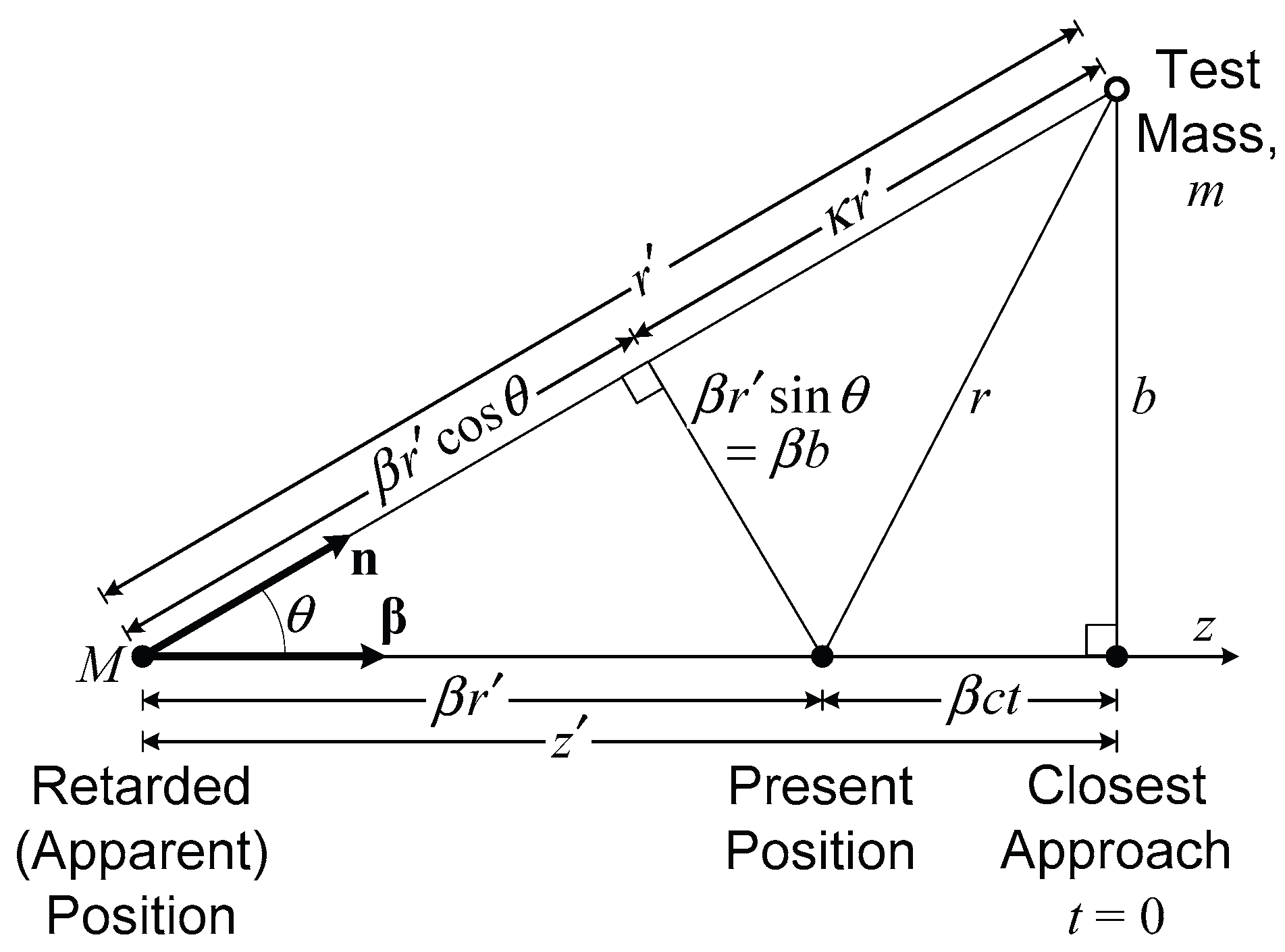
The nonzero metric components of a source in uniform motion, in retarded coordinates, from Refs. [14,15], (C.5), and Fig. E.1, are
,(E.1)
where is the trace of ; the scalar quantity is a retarded Lorentz-transformed range from source mass to test mass; and .
The velocity field of a particle in uniform motion, in retarded coordinates, from (D.6), is
.(E.2)
In electromagnetism, the electric velocity field of a charged particle in uniform motion, from (D.8), corresponding to (E.2), is
.(E.3)
Notice that the Hilbert repulsion term proportional to in the gravitational velocity field in (E.2) is not present in the electric velocity field in (E.3).
With reference to Fig. E.1, the transformation from retarded coordinates, , to present isotropic coordinates for a particle in uniform motion is derived from and , which together imply
and .(E.4)
The transformation from present to retarded coordinates, from Ref. [15] and Fig. E.1, is
and .(E.5)
The inverse transformation from retarded to present coordinates, from Ref. [15] and Fig. E.1, is
and .(E.6)
The transformation from retarded coordinates to present isotropic coordinates, , leaves the scalar range to a test mass m unchanged as , where and , as in Refs. [14,15].
The velocity field in terms of present position, from (E.2) through (E.6) and Ref. [15], is
.(E.7)
This equation predicts gravitational repulsion in present coordinates of a stationary test mass within a forward and backward cone for relativistic source speeds, , corresponding to gravitational repulsion in retarded coordinates from (D.6) and Ref. [15].
In electromagnetism, the electric velocity field in terms of present position, from (E.3) through (E.6) and Ref. [15], corresponding to (E.7), is
.(E.8)
The transverse specific impulse delivered to a test mass by a particle in uniform motion with impact parameter , from (E.7), is
.(E.9)
Since the transverse impulse, , delivered to a test mass is equal and opposite to the impulse delivered to the particle, the angular deflection of the particle in the weak field of the test mass , for , from (E.9), is
.(E.10)
Appendix F. Quadrupole Radiation from a Rotating Binary
This appendix reviews the common derivation of quadrupole gravitational waves produced by a rotating binary, as presented, for example, in Refs. [1,2,3,4]. The interpretation of these waves is that they carry energy and momentum, but do not accelerate masses. Instead, these waves are believed to be curvature ripples on a flat spacetime background that cause coordinates to oscillate past masses, but do not cause the masses themselves to accelerate.
In Appendix H, these quadrupole gravitational waves will be shown to be a linear superposition of dipole waves. Owing to a Doppler modulation effect, the dipole waves from each of the masses of a binary do not completely interfere. The superposition of the dipole waves from each of the masses has the same metric and same angular power distribution as the quadrupole wave from the binary, but the dipole waves do accelerate masses in accordance with the force equation.
The exact solution of the linearized field equation (B.2), from (C.5), is
,(F.1)
where the scalar quantity is a retarded Lorentz-transformed range from source to test mass; is the range from source to test mass; ; is a unit vector pointing from source to test mass; and all quantities within the brackets are evaluated at the retarded time .
The approximate solution in the radiation zone of (B.2) for a nonrelativistic source for which and and , from (F.1), is
.(F.2)
The space and time components of the Hilbert gauge condition with the conservation law , for , are
and .(F.3)
Evaluation of integrals in (F.2), from (F.3) and Ref. [3], gives
.(F.4)
The proof of (F.4) by integration by parts and from (F.3) is
.(F.5)
Evaluation of integrals in (F.4), from (F.3) and Ref. [3], gives
.(F.6)
The proof of (F.6) by integration by parts and from (F.3) is
.(F.7)
Combining (F.4) and (F.6) gives
.(F.8)
Combining (F.2) and (F.8) gives
.(F.9)
To zeroth order in , , and (F.9) is approximately given by
,(F.10)
where is the second derivative with respect to the retarded time of the quadrupole moment; if ; and if . Since the term proportional to does not carry energy, it is omitted from (F.10) and from the calculation of energy flux.
Figure 1 in Sec. 3.1 shows a configuration for calculating the quadrupole radiation of a binary system comprising two particles of masses and moving in circular orbits with constant angular frequency and constant speeds and , respectively, about their center of mass.
The retarded coordinates of and , respectively, from Fig. 1, are
,(F.11)
where and are the constant orbital radii of and , respectively.
The only nonzero components , from (F.10) and (F.11), are
,(F.12)
where is the reduced mass of the binary, and is the distance between the masses.
The only nonzero linearized fields for , from (F.10) and (F.12), are
,(F.13)
where .
The partial time derivatives of the fields, since is nearly constant, from (F.13), are
.(F.14)
The only dependence of on , since is nearly constant, is in the retarded time , so that
,(F.15)
where is the constant radial unit vector in spherical coordinates; and , , and are directional unit vectors at the source.
Using (F.15), the Hilbert gauge condition, , gives
.(F.16)
From (F.14), (F.16) becomes
.(F.17)
The energy-momentum tensor associated with a free gravitational field, from Ref. [3], is given by
.(F.18)
The energy flux of radiation in the radial direction, , for, , , from (F.14), (F.17), and (F.18), is given by
.(F.19)
The energy per unit time per unit solid angle radiated in the radial direction , from (F.19), is
.(F.20)
The total quadrupole power radiated from the rotating binary shown in Fig. 1, from (F.20), is
.(F.21)
Appendix G. Acceleration Field of Relativistic Particles
This appendix derives the exact gravitational acceleration field of a relativistic particle in the radiation zone for . The derivation from the tensor “potential” differs somewhat
from the derivation of the electric acceleration field from the electric vector potential in Ref. [22].
In the source-free radiation zone, in the transverse (Coulomb) gauge. The k-component, , of the gravitational field of a relativistic particle at a stationary test mass in the radiation zone, therefore, from (C.4), is
.(G.1)
The perturbation-metric component in the radiation zone of a relativistic particle with 4-velocity , from (C.5), is
,(G.2)
where the scalar quantity is a retarded Lorentz-transformed range from source to test mass; is the range from the source at to the test mass at ; ; is a unit vector pointing from source to test mass; and all quantities within the brackets are evaluated at the retarded time .
For a particle with mass density , in the integral in (G.2) cannot simply be replaced by in the radiation zone. Instead, similar to (F.4) and (F.6),
.(G.3)
The proof of (G.3) from integration by parts and from the time component of the conservation law, , in the source-free radiation zone, similar to the proofs (F.5) and (F.7), is
.(G.4)
In the radiation zone, the range from source to test mass is approximately constant for a test mass at rest, because . As in Appendix D, for simplicity from this point forward, and are taken to be constants, as they are, for example, for a particle moving at constant speed in a circular orbit.
The perturbation-metric components in the radiation zone, from (G.2) and (G.3), are
,(G.5)
where is the k-component, , of the dipole moment of a particle of mass .
Appendix H. Dipole Radiation from a Rotating Binary
This appendix derives the angular power distribution of gravitational radiation and the total power radiated by a rotating binary in a manner entirely different from the common derivation reviewed in Appendix F.
This appendix shows that a quadrupole gravitational wave radiated by a rotating binary is actually a linear superposition of dipole waves from each of the masses. Owing to a Doppler modulation effect, the dipole waves from each of the masses of a binary do not completely interfere. The superposition of the dipole waves from each of the masses of a binary has the same metric and same angular power distribution as was derived in Appendix F for a quadrupole wave. But the dipole waves accelerate masses in accordance with the force equation of Appendix C, and do not merely produce curvature ripples on a flat spacetime background.
The perturbation-metric components , , in the radiation zone of a binary, from (G.5), are
,(H.1)
where the scalar quantity is a retarded Lorentz-transformed range from source mass to test mass; is the nearly constant range from the source at to the test mass at ; ; is a unit vector pointing from source to test mass; and all quantities within the brackets are evaluated at the retarded time .
The perturbation-metric components , , in the radiation zone of the rotating binary system of particles with masses and shown in Fig. 1, from (G.5) and (H.1), are
,(H.2)
where and are the k-components of the dipole moments; and are the Doppler factors; and are the 4-velocities; and and are the constant Lorentz factors of and .
The coordinates and velocities of and for the binary shown in Fig. 1, from (F.11), are
,(H.3)
where is the constant unit vector in the direction from source to test mass; and are the constant polar and azimuthal angles of the test mass in spherical coordinates; and are the constant orbital radii of and ; and and .
Since the momenta of the masses are equal and opposite and are first order in , to first order in the dipole components of the binary are zero. To second order in , the nonzero dipole components , from (H.2) and (H.3), are
,(H.4)
where ; is the reduced mass of the binary; and is the distance between the masses.
Since is about constant in the radiation zone, the derivative is replaced in (H.4) by because
.(H.5)
Since the components of the dipole wave interference pattern in (H.4) , calculated as a superposition of dipole waves from each mass of a binary, are identical to the components of the quadrupole wave pattern in (F.17), by the Hilbert gauge condition, all the other components of are identical as well. That is, by the Hilbert gauge condition, from (F.14), (F.17), and (H.4), the components are
.(H.6)
Since all the components of the dipole wave interference pattern are identical to the components of the quadrupole wave pattern of Appendix F, the dipole energy per unit time per unit solid angle radiated in the radial direction, from (F.20),
,(H.7)
and the total dipole power radiated from the rotating binary shown in Fig. 1, from (F.21),
,(H.8)
are identical as well.
The difference between the dipole wave interference field, as derived in (H.4) and (H.6), and the quadrupole wave field, as derived in (F.14) and (F.17), is that the dipole field accelerates mass in the radiation zone in accordance with the equation of motion, as seen in App. I.
Appendix I. Dipole Vector Gravitational Field of a Rotating Binary
This appendix derives the dipole gravitational acceleration field in the transverse gauge of the rotating binary shown in Fig. 1 at a stationary test mass in the radiation zone.
In accordance with the equation of motion, (C.4), the acceleration of a test mass at rest at in the source-free radiation zone, by the rotating binary system of particles with masses and shown in Fig. 1, is the dipole vector gravitational acceleration field in the transverse gauge, which from (C.4) and (H.4) is
,(I.1)
where the nomenclature is the same as in Appendix H and
.(I.2)
The dipole field in the radiation zone, from (I.1) and (I.2), is
.(I.3)
By cylindrical symmetry, the field is independent of azimuthal angle . In particular, for , the dipole field in the radiation zone, in the x-z plane of the binary, from (I.3), is
.(I.4)
The transformation from the basis at the binary to the basis at the test mass, where is the direction of propagation of the dipole wave, and as in (I.4), is
.(I.5)
The dipole field propagating in the direction in the transverse gauge at the test mass in the radiation zone, from (I.4) and (I.5), is
.(I.6)
The dipole vector gravitational field (I.6) is the plane-wave vector-field solution of the covariant-vector gravitational field equation (B.8) for slow velocities of the binary shown in Fig. 1 and for the special case in (C.6) of a test mass at rest in the radiation zone.
Appendix J. The Polarization and Power of Vector Gravitational Plane Waves
This appendix is a general treatment of the polarization and power of dipole vector-field plane-wave solutions of the gravitational field equation in the slow-source linear approximation. The treatment is consistent with the common derivation of quadrupole tensor-field plane-wave solutions in the slow-source linear approximation, such as in App. F.
Even though dipole vector fields accelerate masses as in App. I, and do not merely produce curvature ripples on a flat spacetime background as in App. F, a gravitational-wave detector makes no distinction in the linear approximation, as was demonstrated in App. H. In the linear approximation, the perturbation metrics are identical. Nonlinear events, however, like those detected at gravitational-wave observatories, can produce dipole gravitational radiation at the orbital frequency, which is half the quadrupole frequency, as discussed in App. K.
Unit 4-vectors and a wavenumber 4-vector are defined for gravitational plane waves as
, , , , ,(J.1)
where is the angular frequency of the wave.
Transverse traceless polarization tensors are commonly defined for quadrupole gravitational plane waves with as
and .(J.2)
Transverse traceless polarization tensors are defined for dipole gravitational plane waves with as
and .(J.3)
The perturbation metric satisfying the Hilbert gauge condition for dipole gravitational waves in the radiation zone of the binary shown in Fig. 1, from Apps. F and H and (J.1), (J.2), and (J.3), is
,(J.4)
where .
In 3-vector notation, transverse polarization vectors of dipole gravitational plane waves having wavenumber 3-vector , where is a unit vector in the (radial) direction of propagation, are given by the unit 3-vectors,
and .(J.5)
Transverse dipole gravitational and gravimagnetic plane-wave vector fields at a test mass are of the form
,(J.6)
where and are complex amplitudes.
For the dipole vector field in (I.6), of the binary shown in Fig. 1, , and from (I.6) and (J.6),
,(J.7)
so that and in (J.6).
Circularly polarized dipole gravitational plane-wave fields, with positive and negative helicity respectively, are of the form
,(J.8)
where is a complex amplitude.
In the orbital plane, where , the dipole field in (J.7) is linearly polarized. As the test mass approaches the axis of rotation of the binary, where , the polarization approaches circular polarization, though the amplitude of the dipole wave vanishes on the axis, where .
The transverse dipole plane-wave vector fields represented by (J.6) have an instantaneous energy flux of a gravitational acceleration field at a stationary detector in the radiation zone,
,(J.9)
where is the gravimagnetic field.
Poynting’s vector, the instantaneous energy flux of an electromagnetic acceleration field at a stationary detector in the radiation zone, corresponding to (J.9), from Ref. [22], is
,(J.10)
where is the magnetic acceleration field.
The electromagnetic power radiated by the source per unit solid angle, from (J.10), is
.(J.11)
The dipole gravitational power radiated by the source per unit solid angle, corresponding to (J.11), from (I.7) and (J.9), is
.(J.12)
The total dipole power radiated continuously by the rotating binary shown in Fig. 1, obtained by integrating over all solid angle, from (J.12), is
,(J.13)
in agreement with (F.21) and (H.8).
Appendix K. Dipole Radiation from an Isolated Mass Dipole
This appendix calculates the gravitational field and angular distribution of dipole radiation from an isolated accelerating mass dipole in general, and then the radiation for the specific example of a mass caused to move in a circular orbit, for example, by a continuous circularly polarized wave, such as an electromagnetic wave or a dipole gravitational wave.
The perturbation-metric components , , of an isolated mass in the radiation zone, from (G.5), are
,(K.1)
where the scalar quantity is a retarded Lorentz-transformed range from source to test mass; is the nearly constant range from the source at to the test mass at ; is the k-component of the dipole moment; is the Doppler factor; is a unit vector pointing from source to test mass; is the 4-velocity; is the constant Lorentz factor of ; and all quantities within the brackets are evaluated at the retarded time .
To first order in , the nonzero dipole components , from (H.4), (H.5), and (K.1), are
,(K.2)
where an overdot indicates a derivative with respect to the retarded time .
In accordance with the equation of motion, (C.4), the acceleration of a test mass at rest at in the source-free radiation zone, by the particle moving in accordance with (K.2), is the dipole vector gravitational acceleration field in the transverse gauge, from (C.4) and (K.2),
.(K.3)
To the same first order in , the electric acceleration field in the transverse gauge of an isolated charge acting on a test charge at rest at in the source-free radiation zone, corresponding to (K.3), from Ref. [22], is
.(K.4)
Poynting’s vector, the instantaneous energy flux of an electromagnetic acceleration field propagating in the direction to a stationary detector in the radiation zone, from Ref. [22], is
,(K.5)
where is the magnetic acceleration field.
The electromagnetic power radiated by the source per unit solid angle, from (K.5) and Ref. [22], is
,(K.6)
where is the instantaneous angle between and .
The total instantaneous dipole power radiated by the charge , from integrating (K.6) over all solid angle, is the familiar Larmor result for a nonrelativistic accelerated charge, from Ref. [22],
,(K.7)
where is the second time derivative of the electric dipole moment .
The instantaneous energy flux of a gravitational acceleration field propagating in the direction to a stationary detector in the radiation zone, corresponding to (K.5), from (J.9), is
, (K.8)
where is the gravimagnetic field.
The dipole gravitational power radiated per unit solid angle by the isolated mass, corresponding to (K.6), from (K.3) and (K.8), is
(K.9)
where is the instantaneous angle between and .
The total instantaneous dipole power radiated into the radiation zone by the isolated nonrelativistic accelerated mass , corresponding to the familiar Larmor result in (K.7) for a nonrelativistic accelerated charge, from integrating (K.9) over all solid angle, is
,(K.10)
where is the second time derivative of the mass dipole moment .
The dipole gravitational field in (K.3) and the angular power distribution in (K.9) and total dipole power in (K.10) apply generally to any isolated nonrelativistic accelerated mass. As a specific example, the radiation by a mass caused to move at constant speed in a circular orbit by a continuous circularly polarized wave is now calculated.
The coordinates and velocity of an isolated mass moving in a circular orbit of radius and angular frequency are
,(K.11)
where is the constant unit vector in the direction from source to test mass; and are the constant polar and azimuthal angles of the test mass in spherical coordinates; and .
To first order in , the nonzero dipole components , from (K.2) and (K.11), are
.(K.12)
In accordance with the equation of motion, (C.4), the acceleration of a test mass at rest at in the source-free radiation zone, by the particle moving in accordance with (K.2), is the dipole vector gravitational acceleration field in the transverse gauge, from (C.4) and (K.3),
.(K.13)
The transformation from the basis at the binary to the basis at the test mass, where is the direction of propagation of the dipole wave, and , from (I.5), is
.(K.14)
The dipole field propagating in the direction in the transverse gauge at the test mass in the radiation zone, from (K.13) and (K.14), is
.(K.15)
The dipole vector gravitational field (K.15) is the plane-wave vector-field solution of the covariant vector gravitational field equation (B.8) for slow velocities of an isolated mass in constant circular motion and for the special case in (C.6) of a test mass at rest in the radiation zone.
The instantaneous energy flux of the dipole field at a stationary detector in the radiation zone, from (K.8) and (K.15), is
.(K.16)
The dipole gravitational power radiated per unit solid angle by the isolated mass, corresponding to (K.6), from (K.3) and (K.8), is
.(K.17)
The total dipole power radiated continuously by the isolated mass in constant circular motion, obtained by integrating over all solid angle, from (K.17), is
,(K.18)
in agreement with (K.10), and corresponding to the Larmor electromagnetic power formula in (K.7).
Appendix L. Strain Waveform Model for Merger Event GW150914
As shown in (H.4) and (I.6), the dipole gravitational waves from each of the masses of a well-behaved binary, produced at the orbital angular frequency , interfere almost completely. The resulting interference waveform has an angular frequency .
The events detected at gravitational wave observatories are generally mergers of massive compact binaries producing highly nonlinear fields in their source regions. The dipole waves from each of the masses are distorted and delayed by the strong gravitational fields of their companions. These nonlinear effects within the source region disturb the linear interference of the waveforms and leave a trace dipole signal at the orbital angular frequency . A detailed calculation of the dipole radiation at orbital frequency requires numerical relativity.
This appendix shows how a simple waveform model can be used to estimate the dipole radiation power at the orbital frequency produced nonlinearly by the specific merger event, GW150914.
Figure 2 in Sec. 3.4 shows the unfiltered gravitational-wave strain signal of event GW150914 observed by the LIGO Hanford detector. The waveform model focuses only on the eight strain amplitude peaks , , indicated by circles in Fig. 2(a) at
. (L.1)
The quartic-polynomial least-squares fit to these 8 data points,
,(L.2)
indicated by the dashed curve in Fig. 2(a), is considered the envelope of the quadrupole signal amplitude in the waveform model.
As the masses spiral inwards with successively shorter orbital periods, the frequency chirp is modeled by a linearly increasing frequency from each amplitude peak to the next, such that the amplitude peaks in the model occur at exactly the same time as those in the signal, indicated by circles in Fig. 2(a). This provides a continuous orbital angular frequency function for the model.
Figure 2(a) shows an alternating pattern of amplitude peaks above and below the dashed least-squares-fit curve, which suggests that a small dipole signal at orbital frequency could be superposed on the main signal at . The purpose of the strain waveform model is to estimate the order of magnitude of such a possible dipole signal relative to the main signal.
The dipole signal is modeled by a frequency equal to half the main wave frequency and by an amplitude envelope, , equal to the quadrupole amplitude envelope reduced by the constant fraction , which is a parameter in the model. The model of the strain waveform of the superposed quadrupole and dipole waves is
,(L.3)
where s is the time of the initial amplitude peak in Fig. 2.
As shown in Fig. 3, the variance between the model waveform and the actual strain waveform is a minimum for . That is, the model waveform best fits the peak amplitudes of the Hanford LIGO strain signal from the GW150914 event for a dipole signal amplitude at frequency equal to 7.2 percent of the main signal amplitude at . This amplitude corresponds to about 0.5 percent of the power radiated at the orbit frequency. The improvement in the matching of the model with the strain signal by including a superposed dipole signal at the orbit frequency and at amplitude ratio is seen by comparing Fig. 2(a) to 2(b).
Appendix M. Scattering of Dipole Gravitational Waves by a Free Particle
This appendix calculates the total scattering cross section for scattering of unpolarized dipole gravitational radiation by free particles, corresponding to the Thomson cross section for scattering of unpolarized electromagnetic radiation by free charges.
The equation of motion of a free particle of velocity , initially at rest in the radiation zone of an isolated accelerating mass with slow velocity (), in the transverse gauge, from (K.3) is
,(M.1)
where ; is the displacement vector from the retarded source position to the free particle at ; ; is unit vector pointing from the source to the particle; and brackets mean the quantity inside is evaluated at the retarded time .
The dipole gravitational field of a linearly polarized plane wave in the radiation zone produced by a source mass oscillating at angular frequency , from (M.1), is
,(M.2)
where is the wave amplitude; is a unit polarization 3-vector in the direction of , which is transverse to the wavenumber 3-vector .
The dipole gravimagnetic field corresponding to the dipole gravitational field in (M.2), from (K.8), is
.(M.3)
The dipole gravitational power radiated per unit solid angle from a free particle of mass , velocity , and acceleration , for , from (K.9), is
,(M.4)
where is the instantaneous angle between and , a unit vector in the direction of radiation from the free particle.
The time-averaged angular distribution of dipole power radiated from a free particle of mass in the field of a plane dipole gravitational wave , from (M.2) and (M.4), is
.(M.5)
The total dipole power radiated from a free particle, from (K.10), is
.(M.6)
The time-averaged total dipole power radiated from a free particle of mass in the field of the plane dipole gravitational wave , from (M.2) and (M.6), is
.(M.7)
The instantaneous energy flux of the plane dipole gravitational wave in the radiation zone, in the direction of propagation of , from (K.16), is
.(M.8)
The time-averaged energy flux in the direction of propagation of a plane dipole gravitational wave in the radiation zone, from (M.2) and (M.8), is
.(M.9)
The differential scattering cross section for scattering of a plane-polarized dipole gravitational wave by a free particle of mass , if the particle moves a negligible fraction of a wavelength over one oscillation cycle, from (M.5) and (M.9), is
.(M.10)
The differential scattering cross section for scattering of a plane-polarized electromagnetic wave by a particle of mass and charge , corresponding to (M.10), from Ref. [22], is
.(M.11)
The dipole angular distribution , from (K.17) and Ref. [22], is
,(M.12)
where the wave is incident along the axis; the polarization vector makes an angle with the axis; and the direction of radiation is along a polar angle from the axis and an azimuthal angle from the axis.
The differential scattering cross section for scattering of unpolarized dipole gravitational radiation by a free particle of mass , from (M.10) and (M.12), by averaging over , is
.(M.13)
The Thomson formula for scattering of electromagnetic radiation by a free charge , corresponding to (M.13), from Ref. [22], is
.(M.14)
The total scattering cross section for scattering of unpolarized dipole gravitational radiation by a free particle of mass , from (M.13), is
.(M.15)
This cross section is valid only for frequencies at which quantum-mechanical effects are insignificant, that is, for , where is the reduced Planck constant.
The total electromagnetic scattering cross section, called the Thomson cross section, for scattering of unpolarized electromagnetic radiation by a free charge , corresponding to (M.15), from (M.14) and Ref. [22], is
.(M.16)
The Thomson cross section is also valid only for frequencies .
Appendix N. Scattering of Dipole Gravitational Waves by a Mass Oscillator
This appendix calculates the total scattering cross section for scattering of unpolarized dipole gravitational radiation by oscillators at resonance, and the line width of dipole gravitational radiation from oscillators at resonance.
The equation of motion of a simple harmonic oscillator of resonant angular frequency and damping constant , driven by a dipole gravitational wave with constant amplitude and polarization in the direction, is
,(N.1)
where an overdot indicates a derivative with respect to time.
The solution of (N.1) is
, where .(N.2)
The kinetic energy of an oscillator of mass , driven by a dipole gravitational wave , from (N.2), is
,(N.3)
where is the total energy, kinetic plus potential, of the oscillator driven by a dipole gravitational wave of angular frequency .
The line width , defined as the full width at half-maximum (FWHM) energy, from (N.3), is
, (N.4)
where the quality factor is .
Driven at resonant frequency, , the oscillator kinetic energy, from (N.3) and (N.4), is
.(N.5)
Driven at resonant frequency, the oscillator speed and acceleration, from (N.3) and (N.5), are
.(N.6)
Driven at resonant frequency, the oscillator radiates a total dipole power in steady state, from (M.6) and (N.6),
.(N.7)
The time-averaged dipole power radiated from the oscillator at resonance in steady state, from (M.7) and (N.7), is
,(N.8)
where from (M.7) is the time-averaged dipole power radiated from a free particle driven by the same dipole gravitational wave .
The total scattering cross section for scattering of unpolarized dipole gravitational radiation by the oscillator at resonance, from (M.15) and (N.8), is
.(N.9)
The total energy, kinetic plus potential, of the oscillator at resonance, from (N.5), is
. (N.10)
The time-averaged fractional rate of energy radiated by the oscillator at resonance in steady state, from (N.8) and (N.10), is
,(N.11)
which is proportional to the “spring constant” of the oscillator.
From the solution of the homogeneous equation, , the time-averaged total energy of the oscillator at resonance after the driving force is suddenly removed at , from (N.10), is
.(N.12)
The time-averaged rate of fractional energy loss by radiation from the oscillator at resonance after the driving force is suddenly removed at , from (N.11) and (N.12), is
.(N.13)
The FWHM line width of dipole gravitational radiation from the oscillator of mass at resonant frequency , from (N.4) and (N.13), is
,(N.14)
which is proportional to the “spring constant” of the oscillator.
Appendix O. Quantization and Statistics of the Cosmic Gravitational Background (CGB)
This appendix calculates the properties of the CGB assuming it is a collection of spin-1 bosons in thermal equilibrium obeying photon statistics.
If the vector gravitational field of the CGB is regarded as quantized, then the associated spin-1 graviton is a relativistic particle with 4-momentum
,(O.1)
where is the wavenumber 4-vector, and is the reduced Planck constant.
If the CGB is a collection of indistinguishable, massless, spin-1 bosons obeying photon statistics and is in thermal equilibrium at absolute temperature , the mean number of bosons in each state is given by the Planck distribution,
,(O.2)
where is the energy of a boson in state , and is Boltzmann’s constant.
The mode density (number of modes per unit volume) per unit angular frequency for both directions of polarization is identical to that of the cosmic microwave background (CMB),
.(O.3)
The mean number density of spin-1 gravitons per unit angular frequency, in the frequency range from to , from (O.2) and (O.3), is
,(O.4)
where is the energy of a spin-1 graviton in the frequency range from to .
The mean total number density of spin-1 gravitons in all frequencies, found by integrating (O.4), is
,(O.5)
where is the Riemann zeta function (with argument 3).
The mean energy density of spin-1 gravitons per unit angular frequency, in the frequency range from to , from (O.4), is
.(O.6)
The mean energy density of gravitons per unit angular frequency, in (O.6), is a maximum at frequency , corresponding to wavelength , given by Wien’s displacement law,
.(O.7)
The mean total energy density in all frequencies, found by integrating (O.6), is the Stefan-Boltzmann law,
.(O.8)
The mean energy per spin-1 graviton, from (O.5) and (O.8), is
.(O.9)
Appendix P. Fluctuating Gravitational Fields of the CGB from Nyquist Relations
This appendix calculates the energy density of stochastic dipole gravitational fields in thermal equilibrium in the cosmic gravitational background (CGB). The calculation closely follows the derivation of the energy density of stochastic electromagnetic fields in Ref. [49] and gives the same dependence of energy density on dipole gravitational fields as was derived in App. K.
Consider a 1-dimensional oscillator with mass , amplitude , and mass dipole moment,
.(P.1)
The power dissipated through (nonrelativistic) dipole radiation, from (K.10), is
,(P.2)
where .
The power dissipated through dipole radiation, by integration by parts, from (P.2), is
.(P.3)
The dissipative force, from (P.1) and (P.3), is
.(P.4)
The equation of motion of a 1-dimensional oscillator of resonant angular frequency , driven by a dipole gravitational wave of force and polarized in the direction, from (P.1) and (P.4), is
.(P.5)
The time-averaged dipole power radiated from the oscillator at resonance in steady state, from (P.1) and (P.5), is
,(P.6)
in agreement with (N.8).
The oscillator radiation resistance, , the real part of radiation impedance, is the in-phase component of divided by , Ref. [49], from (P.1) and (P.4),
,(P.7)
where is the damping constant from (N.13).
Radiation resistance implies there exists a randomly fluctuating gravitational force in the direction on the mass , and therefore a randomly fluctuating gravitational field , such that, from Ref. [49],
,(P.8)
where and the integral over in (P.8) is .
The mean-square fluctuating gravitational field of the CGB is
,(P.9)
where is the gravimagnetic field from (J.8).
The mean energy density of the CGB, from (J.8), (P.8) neglecting the zero-point contribution, and (P.9), is
,(P.10)
in agreement with the Stefan-Boltzmann law (O.8).
The rms fluctuating gravitational field of the CGB, from (P.10), is
.(P.11)
The mean energy density of the cosmic microwave background (CMB) at equilibrium temperature , corresponding to (P.10), in terms of the root-mean-square (rms) electric and magnetic fields of the CMB, is
.(P.12)
Appendix Q. Drag on Particles in the CGB
This appendix calculates the dipole gravitational radiation of particles moving through the cosmic gravitational background (CGB) and acted on by no forces other than the dipole gravitational forces produced by the stochastic gravitational and gravimagnetic fields of the CGB.
The total instantaneous dipole gravitational power radiated into the radiation zone by an isolated nonrelativistic particle of mass having an acceleration , from Eq. (23), is
. (Q.1)
As shown in Table 1, (Q.1) corresponds to the familiar Larmor result for the total electro mag netic dipole power, , radiated by a nonrelativistic accelerated charge .
The Lorentz invariant generalization of (Q.1) is
, (Q.2)
where the momentum 4-vector of the particle is ; the velocity 3-vector is ; the Lorentz factor is ; is the proper time; and is the proper time element.
The electromagnetic power radiated by an accelerating particle of charge , corresponding to (Q.2), was first obtained by Liénard in 1898, as recounted in Ref. [22], as
. (Q.3)
The proof of the uniqueness of this Lorentz invariant generalization for Larmor radiation power, given in Ref. [22], also applies to dipole gravitational radiation power in (Q.2).
By symmetry in a static, homogeneous universe, the net drag force of the CGB on a particle is expected to be anti-parallel to the velocity of the particle, so from (Q.2),
,(Q.4)
where is the Lorentz factor. For slow particles, (Q.4) agrees with (Q.1).
The manifestly covariant electromagnetic equation of motion is, from Ref. [22],
,(Q.5)
where is the 4-velocity of the charge , and is the electromagnetic field-strength tensor.
In terms of electric and magnetic fields, and , through which the charge is moving, the radiated electromagnetic power, from (Q.3) and (Q.5), is
,(Q.6)
where and are the components of the electric field perpendicular to, and parallel to, the velocity of the charge, and is the component of the magnetic field perpendicular to the velocity of the charge.
In terms of gravitational and gravimagnetic fields, and , through which a mass is moving, the total instantaneous dipole gravitational power, from (Q.2) and App. K, and corresponding to (Q.6), is
,(Q.7)
where and are the components of the gravitational field perpendicular to, and parallel to, the velocity of the mass, and is the component of the gravimagnetic field perpendicular to the velocity of the mass.
The total instantaneous dipole gravitational power radiated by a slow particle, for which and , moving through combined gravitational and gravimagnetic fields, for which is comparable to , from (Q.6), is
for .(Q.8)
For a slow particle, the gravimagnetic field components, and , produce negligible and zero radiated power, respectively, as long as is not much greater than .
The mean dipole gravitational power radiated by a slow particle moving through the stochastic gravitational field of the CGB, from (Q.8), is
.(Q.9)
Numerical simulations confirm that the mean-square stochastic gravitational field of the CGB, , has the same effect on the energy of slow particles over long periods of time as the constant mean-square gravitational field of the CGB, .
Therefore, from (Q.1) and (Q.9), a slow particle moving through the CGB radiates the same dipole gravitational power, independent of velocity, as a particle subject to a constant dissipative deceleration
.(Q.10)
In the CGB at an equilibrium temperature , the blackbody gravitational and gravimagnetic fields of the CGB have a mean energy density , given by the Stefan-Boltzmann law, Eq. (O.8). Therefore, the deceleration, which is the rms fluctuating gravitational field of the CGB, from (P.11), is
.(Q.11)
The next appendix, App. R, calculates the exact metric of a static, homogeneous universe, from which a nondissipative, curvature-related deceleration constant is calculated. In App. S, this nondissipative, curvature-related constant is shown to be an invariant scalar equal to , where is the Hubble constant. In App. T, the dissipative deceleration constant in (Q.11) will be shown to be equal to the curvature-related deceleration constant in a static, homogeneous universe.
Appendix R. Exact Metric of a Static, Homogeneous Universe
This appendix summarizes the derivation of an exact solution in isotropic Cartesian coordinates of Einstein’s equation for a static (time-independent and time-reversible), homogeneous spacetime. In isotropic Cartesian coordinates, , the most general static, homogeneous spacetime interval is
,(R.1)
where is the proper time element; and and are functions of , the displacement 3-vector from the origin .
The general solution of Einstein’s equation for a spacetime interval of the form (R.1) is derived in Ref. [33]. This appendix considers only the simple special case, , of coordinates for which the 3-volume is flat. That is, the only nonvanishing components of the metric tensor are the diagonal components,
.(R.2)
The Christoffel symbols are defined in Ref. [3], for example, as
,(R.3)
where a comma denotes partial differentiation, as for example, . With the metric in (R.2), all but nine of the 64 Christoffel symbols vanish identically,
(R.4)
where a subscript coordinate, ,, or , indicates partial differentiation with respect to that coordinate, as for example, .
The Riemann curvature tensor,
,(R.5)
has the three independent components,
(R.6)
The other components needed for the contraction of the Riemann tensor to the Ricci tensor, , are found from the identities and . Then the only components of the Ricci tensor that do not vanish identically are the diagonal components,
.(R.7)
The curvature scalar , which is the contraction of the Ricci tensor, from (R.7), is
.(R.8)
Ein stein’s equation is
,(R.9)
where is the cosmological constant; , the four-dimensional Kronecker delta, is 1 if and 0 otherwise; is the energy-momen tum tensor; and .
Symmetry requires and . Einstein’s equation requires , and both sides of this equation transform as a scalar only if , so that . Then , and the curvature scalar, from (R.8) and (R.9), is
.(R.10)
A positive energy density, , requires negative curvature, , and negative cosmological constant, .
Any ray from the origin may be defined as the positive axis in Cartesian coordinates, so Einstein’s equation, (R.9), along any ray from the origin becomes
.(R.11)
The exact general solution of (R.11) along any ray from the origin is
,(R.12)
where is an invariant distance from any origin to its event horizon; , or alternatively , is a dimensionless curvature constant; and and are dimensionless constants determined by the boundary conditions, at and at .
Then the exact diagonal metric of a static, homogeneous universe with a flat 3-volume may be expressed in Cartesian coordinates along any ray from the origin, from (R.2) and (R.12), as
.(R.13)
The component of the metric is plotted in Fig. 5 in Sec. 3.9.
Appendix S. Hubble Redshift and Apparent Cosmic Acceleration in a Static Universe
From the metric (R.13), this appendix calculates the effects of a static, homogeneous distribution of energy density throughout a static universe on propagation of light. The spacetime curvature of a static universe causes a time dilation of clocks increasing with their distance that accounts for the Hubble redshift and for an apparent cosmic acceleration. Section 3.12 and App. U show that the appearance of cosmic acceleration in a static universe fits SN-Ia light curve data well for a narrow range of possible energy densities in the static universe.
In isotropic Cartesian coordinates, , the spacetime interval derived in (R.13) for a static, homogeneous universe with a flat 3-volume is
,(S.1)
where is the proper time element. The exact diagonal metric of a static, homogeneous universe with a flat 3-volume, expressed in Cartesian coordinates along any ray from the origin, from (R.13), is
,(S.2)
where is the Cartesian coordinate distance along any ray from the origin; is a convenient function for these calculations; is the distance to the event horizon, at which ; is a dimensionless curvature constant; the curvature scalar is the trace of the Ricci tensor ; and is the homogeneous total energy density of the universe.
The time dilation of clocks at rest in a static universe, , as seen by an observer at rest at the origin, depends upon their distance from the origin, from (S.1) and (S.2), as
.(S.3)
where .
For an observer at rest at the origin in a static, homogeneous universe, the exact redshift parameter, from (S.3), is
.(S.4)
For all over short ranges, , the redshift parameter is linear with range to lowest order in . To second order in , (S.4) becomes
.(S.5)
Over short ranges, the Hubble constant is related to the redshift parameter by , so that for , the Hubble constant is related to the curvature (and energy density) in a static universe, from (S.5), by
,(S.6)
and the redshift parameter in a static universe in terms of the Hubble constant, from (S.5) and (S.6), is expanded to second order in as
.(S.7)
Consider a pulse of light transmitted towards the origin of coordinates from a source at rest at a distance from the origin of coordinates in the rest frame of a static, homogeneous universe. The frequency of light at its source is , and the pulse duration at its source is . When this light pulse reaches an observer at rest at the origin, the frequency of the light will have been redshifted to
,(S.8)
and the pulse duration will have been lengthened to
.(S.9)
That is, time dilation in a static, homogeneous universe will have caused the energy of the light pulse at the coordinate origin to be reduced from the energy at the light source by a factor and the power of the light pulse at the origin to be reduced by a factor from the power of the pulse at the source.
Over short ranges, , the frequency redshift of light in a static universe, as a consequence of the curvature and energy density of the static universe, from (S.6) and (S.8), is given by
,(S.10)
which is just the Hubble redshift, even though the source of light is not moving with respect to the observer at the origin.
From a light source that is moving radially outward from the origin with speed in a flat spacetime, the exact Doppler-redshifted frequency of a light pulse arriving at the origin, from Ref. [22], is
,(S.11)
where is the frequency of the light pulse emitted by the source.
If an observer at rest at the coordinate origin of the rest frame of a static, homogeneous universe misinterprets the light that is redshifted by time dilation from a stationary source as light that is Doppler redshifted by a moving source, then, from (S.8) and (S.11), the stationary source will appear to be moving away from the observer at the origin with an apparent speed given exactly by
.(S.12)
Over short ranges, , the apparent outward speed of the stationary source, from (S.6) and (S.12), is given by
.(S.13)
That is, a stationary source of light, redshifted by time dilation in a static universe, will appear to have an outward speed , given by the Hubble redshift.
To second order in , the apparent speed of a stationary source in a static universe, from (S.6), (S.7) and (S.13), is
.(S.14)
The first term on the right-hand side of (S.14) is an apparent Hubble expansion velocity proportional to distance in a static universe. The second term describes an apparent cosmic acceleration. Appendix U shows that the apparent cosmic acceleration in (S.14) fits the SN-Ia distance modulus data well over a range of from to . But this infinite range of values of corresponds to a narrow range of total density of a static universe. The range of the ratio of the total energy density of a static universe to the critical energy density of a ΛCDM universe, corresponding to , will be shown in App. U to be .
Appendix T. Particle Motion in a Static Universe With CGB Drag
This appendix calculates the combined effects on particle motion, as observed in the rest frame of a static, homogeneous universe, of time dilation derived in App. S with the dissipative drag force of the cosmic gravitational background (CGB). Appendix Q showed that the CGB causes a deceleration of all particles with respect to the rest frame . This dissipative drag force of the CGB is identified in this appendix with the time-dilation drag force of the metric. This identification is possible because the kinetic energy converted to potential energy by the metric, unlike the situation in a time-reversible conservative potential, is nonrecoverable. Then the equation of motion of particles in a static, homogeneous universe relates the Hubble constant to the root-mean-square gravitational field of the CGB.
As in App. S, in isotropic Cartesian coordinates, , the spacetime interval derived in (R.13) for a static, homogeneous universe with a flat 3-volume is
,(T.1)
where is the proper time element. The exact diagonal metric of a static, homogeneous universe with a flat 3-volume, expressed in Cartesian coordinates along any ray from the origin, from (R.13), is
,(T.2)
where is the Cartesian coordinate distance along any ray from the origin; is a convenient function for these calculations; is the distance to the event horizon, at which ; is a dimensionless curvature constant; the curvature scalar is the trace of the Ricci tensor ; and is the homogeneous total energy density of the universe.
Let be the 4-velocity of a particle in the rest frame of a static, homogeneous universe, where an overdot indicates differentiation with respect to the proper time of the particle as, for example, ; is the instantaneous specific 3-momentum of the particle in ; and is a coordinate that keeps track of the total distance traveled by the particle in , so is always nonnegative.
The homogeneous equation of motion of a particle in a static universe is sufficient to calculate the drag on a particle moving through a static, homogeneous universe, just as the Hubble redshift of light was calculated from the metric in App. S. The time-dilation drag effect on particle motion is expressed as a dissipative drag 4-force in a flat spacetime. The drag force applied by the CGB is the physical means by which time-dilation drag is effectuated. As a result of deceleration by the CGB, the particle radiates. The additional energy loss and deceleration of the particle by dipole radiation is calculated at the end of this appendix.
For an observer at rest in , the homogeneous equation of motion of a particle of mass acted on by the time-dilation drag of the metric through the CGB is
,(T.3)
where the are the Christoffel symbols defined at (R.3) and (R.4).
In a static, homogeneous universe, with the metric component given by (T.2), and the Christoffel symbols given by (R.4), the scalar product of the 4-velocity with the homogeneous equation of motion (T.3) is
.(T.4)
The first integral of (T.4) is
,(T.5)
which agrees with the energy equation of the invariant spacetime interval (T.1) with a flat 3-volume.
The time component of the homogeneous equation of motion (T.3) is
.(T.6)
The space components of the homogeneous equation of motion (T.3), from (T.5), are
,(T.7)
where is a unit vector in the direction of the instantaneous particle velocity in .
In terms of a dimensionless specific energy , the energy equation (T.5) becomes
,(T.8)
and the space components of the homogeneous equation of motion (T.7) become
.(T.9)
Differentiating with respect to proper time, from (T.6), gives
, (T.10)
from which the specific energy appears to be a conserved quantity.
Consider a particle radially inbound to an observer at rest at the coordinate origin in a static, homogeneous universe. The particle starts an initial distance from the origin with an initial specific 3-momentum , and has just enough energy to reach the origin before coming to rest there, where and .
For a slow particle () starting close to the origin, (T.8) becomes
.(T.11)
Since is conserved for a particle that comes to rest at the origin, the range is related to the initial specific 3-momentum , from (T.11), by
,(T.12)
showing that the slow particle undergoes a constant deceleration as a result of the time-dilation drag of the metric.
But from (Q.9) and (Q.10), a slow particle moving through the CGB radiates the same dipole gravitational power, independent of velocity, as a particle subject to a constant dissipative deceleration, , where is the constant root-mean-square gravitational field of the CGB. Since the CGB is taken to be the physical mechanism by which the energy of a particle is dissipated as it moves through a static, homogeneous universe, from (Q.10) and (T.12), in a static, homogeneous universe is identified as
.(T.13)
The range of a slow particle before it is brought to rest in a static, homogeneous universe, from (T.12), is . Because the metric has a flat 3-volume, every observer at rest in a static, homogeneous universe will agree on the range of the particle.
The conserved dimensionless specific energy of an ultrarelativistic particle () inbound to an observer at the origin from a short range (), from (T.8), is
.(T.14)
Over short ranges, (T.14) shows that the loss of momentum and energy of an ultrarelativistic particle from time-dilation drag, as a consequence of the curvature and energy density of the static universe, is the same as the loss of momentum and energy (and frequency) of light, given by (S.10). That is, ultrarelativistic particles moving through a static universe experience the same energy loss as light, an energy loss described by the Hubble redshift.
For particles of any initial momentum in a static, homogeneous universe, the range of a particle which has an initial specific 3-momentum , from the energy equation (T.8), is shown in Fig. 6 in Sec. 3.11.
Although the specific energy of a particle moving through the rest frame of a static universe is ostensibly a conserved quantity, the potential energy stored in the gravitational field is nonrecoverable. Reversing the velocity of the particle through does not restore kinetic energy to the particle. Instead, kinetic energy is irrevocably lost no matter which direction the particle moves through a static universe. This behavior is characteristic of a dissipative drag force acting on particles, not of a conservative gravitational potential. Since the time-dilation drag force on a particle acts like a dissipative drag force, rather than the force of a conservative potential, it should be possible to express the time-dilation drag force in the curved spacetime of a static universe as a dissipative drag force in a flat (Minkowski) spacetime, at least over distances short compared to , the length scale of the universe.
So now let be the 4-velocity of a particle in the rest frame of a flat spacetime. For an observer at rest in , the equation of motion of a particle of mass acted on by a dissipative drag 4-force decelerating the particle is
,(T.15)
where is the dissipative drag 4-vector.
In a Minkowski metric, , the scalar product of the 4-velocity with the inhomogeneous equation of motion (T.15) is
.(T.16)
The first integral of (T.16) is
.(T.17)
The energy equation in a Minkowski metric shows from (T.17) that the drag 4-vector must be orthogonal to the particle 4-velocity, that is, .
The dimensionless specific energy of the particle is defined as . Then the time component of the inhomogeneous equation of motion (T.15) is
,(T.18)
and the space components of (T.15) are
.(T.19)
By symmetry in a flat spacetime, any particle that is acted upon only by a drag force will move along a straight trajectory. Since is anti-parallel to by symmetry, and since , then . And since , then the time and space components of the dissipation drag 4-vector are related by
.(T.20)
The time component of the drag 4-vector is a measure of power loss by the particle. For a particle at rest in , and .
If a drag scalar is defined as , then the drag 4-vector, from (T.20), is
,(T.21)
where is a unit vector in the direction of the instantaneous particle velocity in . This drag 4-vector satisfies , , and .
From (T.18) and (T.21),
, (T.22)
which has the exact solution
,(T.23)
where the initial condition was used.
For a slow particle () over a short distance (), (T.23) becomes
,(T.24)
and from (T.24),
,(T.25)
showing that the slow particle undergoes a constant deceleration as a result of the drag force.
For an ultrarelativistic particle () over a short distance (), (T.23) becomes
,(T.26)
so that an ultrarelativistic particle has a deceleration, from (T.26),
.(T.27)
But from (T.9), the deceleration of a particle of any speed over short distances is
.(T.28)
Comparing (T.27) and (T.28) gives the value of the deceleration scalar as
,(T.29)
and the dissipative drag 4-vector over short distances () associated with the 4-velocity of a particle in a static universe, from (T.21) and (T.29), is
.(T.30)
The dissipative equation of motion, , with given by (T.30), emulates the conservative energy equation (T.8), but only over distances much shorter than the cosmological length scale , and only for particles inbound to an observer at the origin. For outbound particles, (T.30) continues to make sense, because it is independent of coordinates and a metric. But for outbound particles, the energy equation (T.8) is unphysical, because there is no conservative potential in a static universe. Kinetic energy can only be lost to the gravitational field; it cannot be recovered.
The instantaneous dipole gravitational power radiated by a particle of mass decelerated by time-dilation drag in a static universe, from (Q.2) and (T.30), is
. (T.31)
and from (T.13), the instantaneous dipole gravitational power radiated by a particle of mass , decelerated by the CGB in a flat universe, is
. (T.32)
Appendix U. Appearance of Cosmic Acceleration in a Static Universe
This appendix calculates the effects of time dilation in a static universe on supernova Type Ia (SN-Ia) light curves. The model of the static universe has only one adjustable parameter, total energy density, and the fit to the SN-Ia light-curve data is good in a narrow range of this parameter.
The energy density of a static universe is related to the curvature scalar defined in (R.8) and to the cosmological constant , from (R.10), by
,(U.1)
where .
Since and , the total energy density of a static universe, including the CGB, from (S.6) and (U.1), is
,(U.2)
where is the Hubble constant, and is the time-dilation deceleration constant from (T.12).
The critical energy density of a lambda-cold-dark-matter (ΛCDM) universe is the energy density below which a ΛCDM universe expands forever, and above which the expansion comes to a stop and reverses. From Ref. [3] and (S.6), this critical energy density is
.(U.3)
The ratio of the total energy density of a static universe to the critical energy density of a ΛCDM universe, from (U.2) and (U.3), is
,(U.4)
showing that a static universe does not support a total energy density greater than .
But since the energy density of a static, homogeneous universe can also be expressed as
,(U.5)
where is the total mass energy of the universe within the radius , including the CGB, the ratio of energy densities in (U.4) can also be expressed as
.(U.6)
Note that is the condition for an event horizon at radius in the isotropic Cartesian coordinates of this static solution, just as is the condition for an event horizon in Schwarzschild coordinates.
From (U.4) and (U.6), , so that the ratio of the total energy density of a static universe to the critical energy density of a ΛCDM universe, from (U.4), is
.(U.7)
Figure 8 in Sec. 3.12 is a plot of the ratio vs. .
The energy density of the CGB, from (P.10), is
.(U.8)
The ratio of the energy density of the CGB to the critical energy density of a ΛCDM universe, from (U.3), (U.8), and (T.13), is
. (U.9)
The ratio of the energy density of the CGB to the total energy density of a static universe including the CGB, from (U.2) and (U.8), is
.(U.10)
Since the energy density of the CGB cannot exceed the total energy density of a static universe including the CGB, the lower bound on , from (U.10), is
, (U.11)
and the lower bound on the Hubble constant, from (S.6) and (U.11), is
.(U.12)
The ratio of the total energy density of a static universe to the critical energy density of a ΛCDM universe, from (U.7) and (U.9), is in the range
,(U.13)
or .
The upper bound on the value of for a static universe, from (U.12), corresponds to , and corresponds to the upper bounds, from (U.1),
.(U.14)
As shown in this appendix below, the cosmological model of a static universe fits the SN-Ia light-curve data quite well with only one adjustable parameter, total energy density (or curvature constant ), and over a broad range of .
From time dilation in a static universe, the frequency of a radially inbound photon observed at the origin is related to the frequency of that photon a distance away, from (S.8), by
.(U.15)
The pulse duration of a bunch of photons is lengthened by time dilation by the same factor as the wavelength of the photons. An incoming bunch of photons with a total energy and total power appears to lose power, from (U.15), as
,(U.16)
where is the absolute total power of the incoming photon bunch measured by an observer at the origin.
Let be the absolute luminosity, the power radiated by a supernova. Let be the apparent luminosity, the power received per unit area at the detector. The ratio, from (U.16), is
,(U.17)
The exact redshift parameter in a static, homogeneous universe, from (S.4), is
.(U.18)
The luminosity ratio in (U.17), from (U.18), becomes
.(U.19)
The apparent magnitude of an SN-Ia is . The absolute magnitude of an SN-Ia is related to its absolute luminosity by . Then the distance modulus, , defined as the difference between the apparent and absolute magnitudes, for an SN-Ia at a distance in a static universe is
,(U.20)
where is an instrument-calibration constant. This distance modulus function in (U.20) of the redshift parameter is shown in Fig. 9 in Sec. 3.12 for several values of the curvature constant in a static universe.
The constant depends only on the calibration of the detectors and not on the features of the model. The best-fit values of the instrument-calibration constant that minimize the sums of squares of deviations of the data points from the distance modulus curves in Fig. 9 are given in Table U.1.

Table U.1.
Best-fit instrument-calibration constants in column 2 that give the least root-mean-square (standard) deviations in column 4 of the distance modulus functions of (U.20) from the data points in Fig. 9 for the curvature constants in column 1. Column 3 shows that is an excellent approximation to the best-fit for all .
Table U.1.
Best-fit instrument-calibration constants in column 2 that give the least root-mean-square (standard) deviations in column 4 of the distance modulus functions of (U.20) from the data points in Fig. 9 for the curvature constants in column 1. Column 3 shows that is an excellent approximation to the best-fit for all .
| Best fit |
Standard deviation |
||
|---|---|---|---|
| 0.1 | 43.78 | 38.47 | 0.466 |
| 1 | 44.22 | 43.47 | 0.394 |
| 2 | 45.08 | 44.98 | 0.349 |
| 3 | 45.86 | 45.86 | 0.343 |
| 4 | 46.48 | 46.48 | 0.342 |
| 5 | 46.96 | 46.96 | 0.342 |
| 10 | 48.46 | 48.47 | 0.342 |
For , the distance modulus curves from (U.20) in Fig. 9 are virtually indistinguishable. The reason is that for , , and over the range of redshift parameter values in Fig. 9, the distance modulus curves from (U.20) in Fig. 9 are approximately given by
.(U.21)
That is, for , the dependence of the distance modulus on is separate from the dependence on , so that an excellent approximation to the best-fit instrument-calibration constant over the range of in Fig. 9 is effectively
,(U.22)
so that the distance modulus curves for are identical, after the constant is adjusted in accordance with (U.22) to the best fit.
The fit of the distance modulus in (U.20) to the data is robust over an unlimited range of this one parameter, from to . Although the distance modulus fits the data well over an infinite range of values of , it fits the data only over a narrow range of total density of a static universe. The range of the ratio of the total energy density of a static universe to the critical energy density of a ΛCDM universe, corresponding to , from (U.4), is
.(U.23)
Appendix V. Hubble Constant, Drag Constant and CGB Temperature
This appendix summarizes some of the recent results of measurements of the Hubble constant, , and relates those measurements to the scalar time-dilation drag constant , and to the temperature of the cosmic gravitational background (CGB).
In Table 3, Sec. 3.13, the dependence of the scalar time-dilation drag constant on the Hubble constant is
.(V.1)
The mean energy density of the CGB, from the Stefan-Boltzmann law (P.10), is
,(V.2)
where is the root-mean-square gravitational field of the CGB in a static universe.
In App. T and specifically at (T.13), it was determined that is related to the Hubble constant by
.(V.3)
Then from (V.1), (V.2), and (V.3), the temperature of the CGB is related to the Hubble constant by
.(V.4)
The temperature of the CGB, according to (V.4), is given for each of the measured values of in the last column of Table 3.
Appendix W. Dipole Anisotropy of the CGB
This appendix calculates the expected anisotropy in the cosmic gravitational background (CGB). If the CGB is a collection of indistinguishable, massless, spin-1 bosons obeying photon statistics and is in thermal equilibrium at absolute temperature , just as the cosmic microwave background (CMB) is, and if the CGB is at rest with respect to the apparent rest frame of the CMB, then the fractional temperature and frequency shifts of the CGB might be expected to be the same as the fractional temperature and frequency shifts of the CMB.
To lowest order in , the normalized speed of the Earth through the CGB, the observed temperature of the CGB with respect to the equilibrium temperature , from Ref. [66], is
,(W.1)
and the apparent temperature shift is
,(W.2)
where is the angle between the boson velocity and the velocity of the Earth through the CGB.
The WMAP satellite experiment [67] found for a velocity of the solar system with respect to the CMB of 370 km/s. If the velocity of the solar system with respect to the CMB is the same with respect to the CGB, then the maximum temperature increase of the CGB would be times the equilibrium temperature of the CGB. From (W.2) and Table 3, the maximum temperature increase of the CGB from the dipole anisotropy is about
. (W.3)
Appendix X. Hubble Constant Related to Planck’s Constant by the CGB
Appendix V, and specifically (V.3) related the scalar time-dilation drag constant in (S.36) for a slow particle moving through a static, homogeneous universe to the dissipative deceleration of a slow particle moving through the root-mean-square gravitational field of the cosmic gravitational background (CGB), by
.(X.1)
One result of (X.1) is that the Hubble constant is related to Planck’s constant , from (Q.11), by
.(X.2)
And the stochastic vector field of the CGB is related to the Hubble constant in turn by (X.1).
The Hubble constant and the rms field of the CGB are related to the equilibrium temperature of the CGB, from (V.3), (V.4), and (X.1), by the relations
.(X.4)
The mean total energy density of the CGB in all frequencies is given by the Stefan-Boltzmann law, from (O.8),
.(X.5)
Table 4, Sec. 3.13, shows the dependence of the mean total energy density of the CGB on the tempera ture from (X.5), and indirectly on the measured values of the Hubble constant from (X.4).
Then with the range of temperatures in Table 4, T = 211 K, corresponding to the range of values of the Hubble constant, , given by Refs. [58,59], the mean total energy density of the CGB, from (X.5), is
;(X.6)
the limit on the total energy density of a static universe, from (U.13), is
;(X.7)
and the critical energy density of a lambda-cold-dark-matter (ΛCDM) universe, from (U.3), is
.(X.8)
The ratio of the energy density of the CGB to the critical energy density of a ΛCDM universe, from (U.9), is
, (X.9)
and the ratio of to the total energy density of a static universe including the CGB, from (U.10), is
.(X.10)
But if is greater than 2, as suggested by App. U, then, from (X.10),
.(X.11)
And in that case, any other constituent of a static universe, like ordinary mass, has an energy density satisfying
,
or
.(X.12)
That is, ordinary mass in a static universe has an energy density no more than about 4.0 to 5.5 percent of the critical energy density of a ΛCDM universe. This small energy density of ordinary mass corresponds to the energy density of ordinary mass in our universe of 4.9 percent of the critical energy density of a ΛCDM universe, for example, as inferred by Ref. [57], and as shown graphically in Fig. 10 in Sec. 3.12.
Appendix Y. Mean Energy of an Oscillator in the CGB
The stochastic gravitational vector fields of the cosmic gravitational background (CGB) will cause every particle to undergo stochastic motion, in accordance with the equation of motion, Eq. (24). This appendix calculates an effective diffusion coefficient from the mean energy of an oscillator of resonant frequency in the CGB at equilibrium temperature . The oscillator is driven by the stochastic dipole gravitational fields of the CGB and its motion is damped by dipole radiation produced by its own acceleration.
In App. N, the derivation of the mean energy of mass oscillators in the CGB closely followed the derivation of the mean energy of oscillators in electromagnetic fields from the generalized Nyquist relation in Ref. [49]. To recap results of App. N, the displacement of a one-dimensional simple harmonic oscillator of mass , resonant angular frequency , and damping constant , driven by a dipole gravitational wave with constant amplitude and polarization in the direction, satisfies the equation of motion (N.1), and the solution of (N.1) is given by (N.2).
When driven at the resonant frequency, , the displacement of the mass , from (N.2), is
,(Y.1)
and the velocity is
.(Y.2)
The damping constant was found at (N.13) to be
.(Y.3)
When driven by a dipole gravitational wave at the resonant frequency, the total energy of the oscillator of mass , kinetic plus potential, from (Y.2), is
.(Y.4)
The line width , defined as the full width at half-maximum (FWHM) of the energy spectrum of the oscillator for , was found from (N.14) to be
.(Y.5)
Defined in this way, the line width is equal to the damping constant of an oscillator in the CGB.
The root-mean-square (rms) displacement of the oscillator from (Y.1) is . The root-mean-square speed of the oscillator from (Y.2) is . The “diffusion coefficient,” , of the oscillator is defined as the product in the CGB of “uncertainty” of oscillator position, , and “uncertainty” of oscillator speed, , or from (Y.4),
.(Y.6)
If is the zero-point energy of the one-dimensional oscillator, , then the “diffusion coefficient” from (Y.6) is
. (Y.7)
According to Ref. [69], any particle of mass that is constantly undergoing a Brownian motion with diffusion coefficient obeys the Schrödinger wave equation. One might therefore conclude from (Y.7) and Ref. [69] that an oscillator immersed in the CGB obeys the Schrödinger wave equation.
Following is an approximate derivation of the diffusion coefficient of an oscillator immersed in the CGB that involves somewhat less circular reasoning than the derivation of (Y.7). According to Planck’s second quantum theory [117], the mean energy at the temperature of an oscillator at natural frequency is
.(Y.8)
In the CGB, the mean-square gravitational field polarized in the direction, from the Nyquist relations, is
.(Y.9)
Only the CGB modes roughly within the frequency band about the resonant frequency contribute significantly to the resonant amplitude of the oscillator. Consider an in-band plane-wave dipole gravitational field of the CGB,
for ,(Y.10)
propagating in the direction, comprising field modes of both polarizations, where is the amplitude, is the angular frequency, and is the phase of the field mode.
As long as and , then from Ref. [33] the field modes within the narrow resonant frequency band about combine to produce effectively a single mode with an angular frequency about equal to and with an amplitude , where is the mean amplitude of each of the modes in the narrow band. That is, within the frequency band about , the driving field at a particular location is
,(Y.11)
where is some phase angle.
Thus, the in-band gravitational wave amplitude from (Y.1) and (Y.11) is approximately related to the in-band mean-square gravitational field, from (Y.9), by
.(Y.12)
At high resonant frequencies (), the mean energy of the oscillator is , the zero-point energy of the oscillator. Then using and using (Y.5) for the line width and for the damping constant , the in-band mean-square gravitational field from (Y.12) becomes
.(Y.13)
Then the approximate diffusion coefficient of a 1-dimensional oscillator immersed in the CGB, from (Y.6) and (Y.13), is
.(Y.14)
The reason the approximate diffusion coefficient in (Y.14) underestimates the diffusion coefficient in (Y.7) by a factor is because only those dipole wave modes within a bandwidth about the resonant frequency were taken to contribute to the gravitational wave driving the oscillator at resonance.
The diffusion coefficient of the one-dimensional oscillator in the CGB from (Y.6) is , which is independent of the stochastic vector field that produced it. The diffusion coefficient of a one-dimensional charged-particle oscillator in the stochastic electromagnetic field of the cosmic microwave background (CMB) is the same as it is in the CGB, . The reason is that the mean energy density of the CGB, from (P.10),
,(Y.15)
is the same as the mean energy density of the CMB, from (P.12),
,(Y.16)
differing only in the absolute temperature of the stochastic vector field.
And for the same reasons, the mean energy in the CGB of a one-dimensional, charged or uncharged particle oscillator at natural frequency , from (Y.8), is
,(Y.17)
while the mean energy in the CMB of a one-dimensional, charged particle oscillator at natural frequency , is
,(Y.18)
again differing only in the absolute temperature of the stochastic vector field.
At high resonant frequencies (), the mean energy of a one-dimensional charged particle oscillator is the zero-point energy of the oscillator, , in either the CGB or the CMB or both. At high frequencies, the mean energy is completely independent of the stochastic vector field that determines it. The only differences in the mean energy of oscillators arise for weakly bound or free particles, that is, for less than or about equal to .
If , then the mean energy in the CGB of a one-dimensional oscillator, from (Y.17), is about , and the mean energy in the CMB, from (Y.18), is about , differing only in the absolute temperature of the stochastic vector field. Since the absolute temperature of the CMB is and the absolute temperature of the CGB in a static universe is about , as shown in Table 3, the mean energy in a combined CGB and CMB of a free or weakly-bound, charged or uncharged, one-dimensional particle oscillator with , from Eq. (90), is about , as shown in Fig. 11, Sec. 3.14.
References
- See, for example, Landau, L.D. and Lifshitz, E.M. In The Classical Theory of Fields, 4th Revised English Ed.; Elsevier Ltd: Oxford, 1975.
- See; for example; Misner, C.W.; Thorne, K.S.; Wheeler, J.A. Gravitation; WH Freeman & Co: San Francisco, 1973. [Google Scholar]
- See, for example, Ohanian, H., Ruffini, R.: Gravitation and Spacetime. In Gravitation and Spacetime, 2nd Ed. 3rd Ed. ed; W.W. Norton & Co.: New York; Cambridge University Press: New York, 1994.
- See, for example, Carroll, S.M. In Spacetime and Geometry; Cambridge University Press: Cambridge, 2019.
- Flanagan, É.É.; Hughes, S.A. The basics of gravitational wave theory. New J. Phys. 2005, 7, 204–255. [Google Scholar] [CrossRef]
- Williams, L.L.; Inan, N. Maxwellian mirages in general relativity. New J. Phys. 2021, 23, 053019. [Google Scholar] [CrossRef]
- Braginsky, V.B.; Caves, C.M.; Thorne, K.S. Laboratory experiments to test relativistic gravity. Phys. Rev. D. 1977, 15, 2047–2068. [Google Scholar] [CrossRef]
- Harris, E.G. Analogy between general relativity and electromagnetism for slowly moving particles in weak gravitational fields. Am. J. Phys. 1991, 59, 421–425. [Google Scholar] [CrossRef]
- Ciufolini, I.; Wheeler, J.A. Gravitation and Inertia; Princeton University Press: Princeton, 1995. [Google Scholar]
- Mashhoon, B. Time-varying gravitomagnetism. Class. Quantum Grav. 2008, 25, 085014. [Google Scholar] [CrossRef]
- Bini, D.; Cherubini, C.; Chicone, C.; Mashhoon, B. Gravitational induction. Class. Quantum Grav. 2008, 25, 225014. [Google Scholar] [CrossRef]
- Kerr, R.P.: Gravitational field of a spinning mass as an example of algebraically special metrics. Phys. Rev. Lett. 11, 237–238 (1963); Boyer, R.H., Lindquist, R.W.: Maximal analytic extension of the Kerr metric. J. Math. Phys. 8, 265–281 (1967).
- Chandrasekhar, S. The Mathematical Theory of Black Holes; Oxford University Press: New York, 1983. [Google Scholar]
- Hartle, J.B.; Thorne, K.S.; Price, R.H. Gravitational interaction of a black hole with distant bodies. In Black Holes: The Membrane Paradigm; Thorne, K.S., Price, R.H., Macdonald, D.A., Eds.; Yale University Press: New Haven, 1986; pp. 146–180. [Google Scholar]
- Felber, F. Test of relativistic gravity for propulsion at the Large Hadron Collider. AIP Conf. Proc. 2010, 1208, 247–259. [Google Scholar] [CrossRef]
- Hilbert, D. Die Grundlagen der Physik. Math. Ann. 1924, 92, 1–32. [Google Scholar] [CrossRef]
- Carmeli, M. Behaviour of fast particles in the Schwarzschild field. Lett. Al Nuovo Cim. 1972, 3.9, 379–383. [Google Scholar] [CrossRef]
- McGruder, C.H. Gravitational repulsion in the Schwarzschild field. Phys. Rev. D. 1982, 25, 3191–3194. [Google Scholar] [CrossRef]
- Mashhoon, B. Beyond gravitoelectromagnetism: critical speed in gravitational motion. Int. J. Mod. Phys. D. 2005, 14, 2025–2037. [Google Scholar] [CrossRef]
- Kopeikin, S.M.; Schäfer, G. Lorentz covariant theory of light propagation in gravitational fields of arbitrary-moving bodies. Phys. Rev. D. 1999, 60, 124002. [Google Scholar] [CrossRef]
- Felber, F. Exact relativistic ‘antigravity’ propulsion. AIP Conf. Proc. 2006, 813, 1374–81. [Google Scholar] [CrossRef]
- See, for example, Jackson, J.D.: Classical Electrodynamics. In Classical Electrodynamics, 2nd Ed. ed; John Wiley & Sons: New York, 1962.
- Thirring, W. Principles of Quantum Electrodynamics; Bernstein, J., Translator; Academic: New York, 1958. [Google Scholar]
- Felber, F. Dipole gravity waves from unbound quadrupoles. arXiv 2010, arXiv:1002.0351. [Google Scholar] [CrossRef]
- Jansen, R.H.; Dever, T.P. G2 flywheel module design. NASA/CR–2006-213862, AIAA-2004-5603 (2006). 2006. Available online: https://ntrs.nasa.gov/api/citations/20060028492/downloads/20060028492.pdf (accessed on 21 April 2025).
- Bonnor, W.B.; Rotenberg, M.A. Transport of momentum by gravitational waves: the linear approximation. Proc. R. Soc. Lond. A 1961, 265, 109–116. [Google Scholar] [CrossRef]
- Peres, A. Classical radiation recoil. Phys. Rev. 1962, 128, 2471–2475. [Google Scholar] [CrossRef]
- Bekenstein, J.D. Gravitational-radiation recoil and runaway black holes. Astrophys. J. 1973, 183, 657–664. [Google Scholar] [CrossRef]
- Wiseman, A.G. Coalescing binary systems of compact objects to (post)5/2-Newtonian order. II. Higher-order wave forms and radiation recoil. Phys. Rev. D. 1992, 46, 1517–1539. [Google Scholar]
- Favata, M.; Hughes, S.A.; Holz, D.E. How black holes get their kicks: gravitational radiation recoil revisited. Astrophys. J. 2004, 607, L5–L8. [Google Scholar] [CrossRef]
- Thorne, K.S. Multipole expansions of gravitational radiation. Rev. Mod. Phys. 1980, 52, 299–339. [Google Scholar] [CrossRef]
- Fitchett, M.J. The influence of gravitational wave momentum losses on the centre of mass motion of a Newtonian binary system. MNRAS 1983, 203, 1049–1062. [Google Scholar] [CrossRef]
- Felber, F. Einstein’s Inertial Field; Starmark Physics: San Diego, 2016. [Google Scholar]
- See, for example, Ref. pp. 394–401.
- Lense, J.; Thirring, H. On the gravitational effects of rotating masses: The Thirring-Lense papers. In Gen. Rel. Grav.; Mashhoon, B.; Hehl, F.W.; Theiss, D.S., Translators; 1984; Volume 16, pp. 711–750. [Google Scholar]
- Abbott, B.P.; Abbott, R.; Abbott, T.D.; Abernathy, M.R.; Acernese, F.; Ackley, K.; Adams, C.; Adams, T.; Addesso, P.; Adhikari, R.X.; et al. Observation of gravitational waves from a binary black hole merger. Phys. Rev. Lett. 2016, 116, 061102. [Google Scholar] [CrossRef] [PubMed]
- Aasi, J.; Abbott, B.P.; Abbott, R.; Abbott, T.; Abernathy, M.R.; Ackley, K.; Adams, C.; Adams, T.; Addesso, P.; Adhikari, R.X.; et al. Advanced LIGO. Class. Quantum Grav. 2015, 32, 074001. [Google Scholar] [CrossRef]
- Einstein, A. Näherungsweise Integration der Feldgleichungen der Gravitation. Sitzungsber. K. Preuss. Akad. Wiss. 1916, 1, 688–696. [Google Scholar]
- Einstein, A. Über Gravitationswellen. Sitzungsber. K. Preuss. Akad. Wiss. 1918, 1, 154–167. [Google Scholar]
- Hulse, R.A.; Taylor, J.H. Discovery of a pulsar in a binary system. Astrophys. J. 1975, 195, L51–L53. [Google Scholar] [CrossRef]
- Taylor, J.H., Weisberg, J.M.: A new test of general relativity – Gravitational radiation and the binary pulsar PSR 1913+16. Astrophys. J. 253, 908 (1982); Further experimental tests of relativistic gravity using the binary pulsar PSR 1913+16. Astrophys. J. 345, 434 (1989).
- Weisberg, J.M.; Huang, Y. Relativistic measurements from timing the binary pulsar PSR B1913+16. Astrophys. J. 2016, 829, 55. [Google Scholar] [CrossRef]
- Dong, S.; Shappee, B.J.; Prieto, J.L.; Jha, S.W.; Stanek, K.Z.; Holoien, T. W.-S.; Kochanek, C.S.; Thompson, T.A.; Morrell, N.; Thompson, I.B.; et al. ASASSN-15lh: A highly super-luminous supernova. Science 2016, 351, 257. [Google Scholar] [PubMed]
- Felber, F. Dipole radio-frequency power from laser plasmas with no dipole moment. Appl. Phys. Lett. 2005, 86, 231501. [Google Scholar] [CrossRef]
- Shapiro, I.I. Fourth test of general relativity. Phys. Rev. Lett. 1964, 13, 789. [Google Scholar] [CrossRef]
- See; for example; Einstein, A. Lens-like action of a star by the deviation of light in the gravitational field. Science 1936, 84, 506–507. [Google Scholar] [CrossRef] [PubMed]
- Chatziioannou, K.; Cotesta, R.; Ghonge, S.; Lange, J.; Ng, K.K.Y.; Bustillo, J.C.; Clark, J.; Haster, C.-J.; Khan, S.; Pürrer, M.; et al. On the properties of the massive binary black hole merger GW170729. Phys. Rev. D. 2019, 100, 104015. [Google Scholar] [CrossRef]
- Abbott, R.; Abbott, T.D.; Abraham, S.; Acernese, F.; Ackley, K.; Adams, C.; Adhikari, R.X.; Adya, V.B.; Affeldt, C.; Agathos, M.; et al. GW190412: Observation of a binary-black-hole coalescence with asymmetric masses. Phys. Rev. D. 2020, 102, 043015. [Google Scholar]
- Callen, H.B.; Welton, T.A. Irreversibility and generalized noise. Phys. Rev. 1951, 83, 34–40. [Google Scholar] [CrossRef]
- Nyquist, H. Thermal agitation of electric charge in conductors. Phys. Rev. 1928, 32, 110–113. [Google Scholar] [CrossRef]
- Mather, J.C.; Fixsen, D.J.; Shafer, R.A.; Mosier, C.; Wilkinson, D.T. Calibrator design for the COBE* Far Infrared Absolute Spectrophotometer (FIRAS). Astrophys. J. 1999, 512, 511. [Google Scholar]
- Felber, F. Cosmic, galactic, and geomagnetic fields sharply limit electron cosmic ray energies. Bull. Am. Phys. Soc. Proc. 2021 APS April Meeting, 17-20 April 2021; 2021. Abstract SP01.003 Bibcode: 2021APS..APRSP1033F. [Google Scholar]
- Pound, R.V.; Rebka, G.A. Apparent weight of photons. Phys. Rev. Lett. 1960, 4, 337–341. [Google Scholar] [CrossRef]
- Pound, R.V.; Snider, J.L. Effect of gravity on nuclear resonance. Phys. Rev. Lett. 1964, 13, 539–540. [Google Scholar] [CrossRef]
- Pound, R.V.; Snider, J.L. Effect of gravity on gamma radiation. Phys. Rev. B 1965, 140, 788–803. [Google Scholar] [CrossRef]
- Hicken, M.; Wood-Vasey, W.M.; Blondin, S.; Challis, P.; Jha, S.; Kelly, P.L.; Rest, A.; Kirshner, R.P. Improved dark energy constraints from ~100 new CfA supernova Type Ia light curves. Astrophys. J. 2009, 700, 1097–1140. [Google Scholar] [CrossRef]
- Planck Collaboration; Aghanim, N.; Akrami, Y.; Ashdown, M.; Aumont, J.; Baccigalupi, C.; Ballardini, M.; Banday, A.J.; Barreiro, R.B.; Bartolo, N.; Basak, S.; et al. Planck 2018 results - VI. Cosmological parameters. Astron. Astrophys. 2020, 641, A6. [Google Scholar] [CrossRef]
- Ferrarese, L.; Gibson, B.; Kelson, D.; Sakai, S.; Mould, J.; Freedman, W.; Kennicutt, R.; Ford, H.; Graham, J.; Huchra, J.; et al. The Hubble constant from the HST Key Project on the extragalactic distance scale. In Proc. Cosmic Flows Workshop ASP Conference Series; Victoria, Canada, Courteau, S., Strauss, M., Willick, J., Eds.; July 1999. [Google Scholar] [CrossRef]
- Freedman, W.L.; Madore, B.F.; Gibson, B.K.; Ferrarese, L.; Kelson, D.D.; Sakai, S.; Mould, J.R.; Kennicutt, R.C.; Ford, H.C.; Graham, J.A.; et al. Final results from the Hubble Space Telescope Key Project to measure the Hubble constant. Astrophys. J. 2001, 553, 47. [Google Scholar] [CrossRef]
- Riess, A.G.; Yuan, W.; Macri, L.M.; Scolnic, D.; Brout, D.; Casertano, S.; Jones, D.O.; Murakami, Y.; Anand, G.S.; Breuval, L.; et al. A comprehensive measurement of the local value of the Hubble constant with 1 km s−1 Mpc−1 uncertainty from the Hubble Space Telescope and the SH0ES Team. Astrophys. J. Lett. 2022, 934, L7. [Google Scholar] [CrossRef]
- Kelly, P.L.; Rodney, S.; Treu, T.; Oguri, M.; Chen, W.; Zitrin, A.; Birrer, S.; Bonvin, V.; Dessart, L.; Diego, J.M.; et al. Constraints on the Hubble constant from supernova Refsdal’s reappearance. Science 2023, 380(Issue 6649). [Google Scholar] [CrossRef]
- Madhavacheril, M.S.; Qu, F.J.; Sherwin, B.D.; MacCrann, N.; Li, Y.; Abril-Cabezas, I.; Ade, P.A.R.; Aiola, S.; Alford, T.; Amiri, M.; et al. The Atacama Cosmology Telescope: DR6 gravitational lensing map and cosmological parameters. Astrophys. J. 2024, 962, 113. [Google Scholar] [CrossRef]
- Scolnic, D.; Riess, A.G.; Wu, J.; Li, S.; Anand, G.S.; Beaton, R.; Casertano, S.; Anderson, R.I.; Dhawan, S.; Ke, X. CATS: The Hubble constant from standardized TRGB and Type Ia Supernova measurements. 2023. [CrossRef]
- Smoot, G.F.; Bennett, C.L.; Kogut, A.; Aymon, J.; Backus, C.; De Amici, G.; Galuk, K.; Jackson, P.D.; Keegstra, P.; Rokke, L.; et al. Preliminary results from the COBE Differential Microwave Radiometers: Large angular scale isotropy of the cosmic microwave background. Astrophys. J. 1991, 371, L1–L5. [Google Scholar] [CrossRef]
- Kogut, A.; Lineweaver, C.; Smoot, G.F.; Bennett, C.L.; Banday, A.; Boggess, N.W.; Cheng, E.S.; De Amici, G.; Fixsen, D.J.; Hinshaw, G.; et al. Dipole anisotropy in the COBE Differential Microwave Radiometers first-year sky maps. Astrophys. J. 1993, 419, 1–6[a]. [Google Scholar] [CrossRef]
- Weinberg, S. Cosmology; Oxford University Press: New York, 2008; pp. 129–132. [Google Scholar]
- Bennett, C.L.; Halpern, M.; Hinshaw, G.; Jarosik, N.; Kogut, A.; Limon, M.; Meyer, S.S.; Page, L.; Spergel, D.N.; Tucker, G.S.; et al. First-year Wilkinson Microwave Anisotropy Probe (WMAP) observations: Preliminary maps and basic results. Astophys. J. Suppl. 2003, 148, 1–27. [Google Scholar]
- Sakharov, A.D. Vacuum quantum fluctuations in curved space and the theory of gravitation. Sov. Phys. – Dokl. 1968, 12, 1040–1041. [Google Scholar]
- Nelson, E. Derivation of the Schrödinger equation from Newtonian mechanics. Phys. Rev. 1966, 150, 1079–85. [Google Scholar] [CrossRef]
- De, S.; Chakrabarty, S. Schrödinger equation of a particle in a uniformly accelerated frame and the possibility of a new kind of quanta. Mod. Phys. Lett. A 2015, 30, 1550182. [Google Scholar] [CrossRef]
- Le Verrier, U. 1859 Lettre de M. Le Verrier à M. Faye sur la théorie de Mercure et sur le mouvement du périhélie de cette planète. Comptes Rendus Hebd. Des. Séances De l'Académie Des. Sci. 1859, 49, 379–383. [Google Scholar]
- Einstein, A. Erklärung der Perihelbewegung des Merkur aus der allgemeinen Relativitätstheorie. Preuss. Akad. Wiss. Berl. Sitzber. 1915, 831–839. [Google Scholar]
- Einstein, A. Die Feldgleichungen der Gravitation. Preuss. Akad. Wiss. Berl. Sitzber. 1915, 47, 844–847. [Google Scholar]
- Dyson, F.W.; Eddington, A.S.; Davidson, C. A determination of the deflection of light by the Sun’s gravitational field, from observations made at the total eclipse of May 29, 1919. Philos. Trans. R. Soc. A Math. Phys. Eng. Sci. 1920, 220, 291–333. [Google Scholar] [CrossRef]
- Durrer, R. The cosmic microwave background: the history of its experimental investigation and its significance for cosmology. Class. Quantum Grav. 2015, 32, 124007. [Google Scholar] [CrossRef]
- McKellar, A. Evidence for the molecular origin of some hitherto unidentified interstellar lines. Pub. Ast. Soc. Pac. 1940, 52, 187–192. [Google Scholar] [CrossRef]
- Adams, W.S. Recent results in stellar spectroscopy. Pub. Ast. Soc. Pac. 1941, 53, 209–218. [Google Scholar] [CrossRef]
- Penzias, A.A.; Wilson, R.W. A measurement of excess antenna temperature at 4080 Mc/s. Astrophys. J. 1965, 142, 419–421. [Google Scholar]
- Roth, K.C.; Meyer, D.M.; Hawkins, I. Interstellar cyanogen and the temperature of the cosmic microwave background radiation. Astrophys. J. Lett. 1993, 413, L67–L71. [Google Scholar] [CrossRef]
- Anderson, J.D.; Laing, P.A.; Lau, E.L.; Liu, A.S.; Nieto, M.M.; Turyshev, S.G. Study of the anomalous acceleration of Pioneer 10 and 11. Phys. Rev. D. 2002, 65, 082004. [Google Scholar] [CrossRef]
- Nieto, M.M.; Anderson, J.D. Search for a solution of the Pioneer anomaly. Contemp. Phys. 2007, 48, 41–54. [Google Scholar] [CrossRef]
- Hewitt, A.; Burbidge, G.; Fang, L.Z. (Eds.) See, for example, Sancisi, R., van Albada, T.S.: Dark Matter. In Observational Cosmology; Springer: Dordrecht, 1987; Volume IAUS 124, pp. 699–712. [Google Scholar] [CrossRef]
- See, for example, Sanders, R.H.: The Dark Matter Problem, a Historical Perspective; Cambridge University Press: Cambridge, 2010.
- See; for example; Milgrom, M. A modification of Newtonian dynamics as a possible alternative to the hidden matter hypothesis. Astrophys. J. 1983, 270, 365–370. [Google Scholar] [CrossRef]
- See; for example; Milgrom, M. MOND theory. Canad. J. Phys. 2015, 93, 107–118. [Google Scholar] [CrossRef]
- Schwarzschild, K. Über das Gravitationsfeld eines Massenpunktes nach der Einsteinschen Theorie. Sitzber. Deut. Akad. Wiss. Berl. Kl. Math.-Phys. Tech. 1916, 189–196. [Google Scholar]
- Schwarzschild, K. Über das Gravitationsfeld einer Kugel aus inkompressibler Flussigkeit nach der Einsteinschen Theorie. Sitzber. Deut. Akad. Wiss. Berl. Kl. Math.-Phys. Tech. 1916, 424–434. [Google Scholar]
- Einstein, A. Kosmologische Betrachtungen zur allgemeinen Relativitätstheorie. Preuss. Akad. Wiss. Berl. Sitzber. Reprinted in English in. 1917, 142–152. [Google Scholar]
- Lorentz, H.A.; Einstein, A.; Minkowski, H.; Weyl, H. The Principle of Relativity: A Collection of Original Memoirs on the Special and General Theory of Relativity; Dover Publications: New York, 1923. [Google Scholar]
- Robertson, H.P. Relativistic cosmology. Rev. Mod. Phys. 1933, 5, 62–90. [Google Scholar] [CrossRef]
- See; for example; Griffiths, J.B.; Podolsky, J. Exact Space-Times in Einstein’s General Relativity; Cambridge University Press: Cambridge, 2009. [Google Scholar]
- Dyson, F. A meeting with Enrico Fermi. Nature 2004, 427, 297. [Google Scholar] [CrossRef] [PubMed]
- Zwicky, F. On the red shift of spectral lines through interstellar space. Proc. Nat. Acad. Sci. 1929, 15, 773–779. [Google Scholar] [PubMed]
- Shamir, L. An empirical consistent redshift bias: A possible direct observation of Zwicky’s TL theory. Particles 2024, 7, 703–716. [Google Scholar] [CrossRef]
- Cowley, W.I.; Baugh, C.M.; Cole, S.; Frenk, C.S.; Lacey, C.G. Predictions for deep galaxy surveys with JWST from ΛCDM. Mon. Not. R. Astron. Soc. 2018, 474, 2352–2372. [Google Scholar]
- Neeleman, M.; Prochaska, J.X.; Kanekar, N.; Rafelski, M. A cold, massive, rotating disk galaxy 1.5 billion years after the Big Bang. Nature 2020, 581, 269–272. [Google Scholar] [CrossRef] [PubMed]
- Curtis-Lake, E.; Carniani, S.; Cameron, A.; Charlot, S.; Jakobsen, P.; Maiolino, R.; Bunker, A.; Witstok, J.; Smit, R.; Chevallard, J.; et al. Spectroscopic confirmation of four metal-poor galaxies at. Nat. Astron. 2023, 7, 622–632. [Google Scholar] [CrossRef]
- Whitler, L.; Endsley, R.; Stark, D.P.; Topping, M.; Chen, Z.; Charlot, S. On the ages of bright galaxies 500 Myr after the big bang: Insights into star formation activity at with JWST. Mon. Not. R. Astron. Soc. 2023, 519, 157–171. [Google Scholar]
- Glazebrook, K.; Nanayakkara, T.; Schreiber, C.; Lagos, C.; Kawinwanichakij, L.; Jacobs, C.; Chittenden, H.; Brammer, G.; Kacprzak, G.G.; Labbe, I.; et al. A massive galaxy that formed its stars at. Nature 2024, 628, 277–281. [Google Scholar] [CrossRef] [PubMed]
- Yu, H.-R.; Zhang, T.-J.; Pen, U.-L. Method for direct measurement of cosmic acceleration by 21-cm absorption systems. Phys. Rev. Lett. 2014, 113, 041303. [Google Scholar] [CrossRef] [PubMed]
- Sandage, A. The change of redshift and apparent luminosity of galaxies due to the deceleration of selected expanding universes. Astrophys. J. 1962, 136, 319. [Google Scholar] [CrossRef]
- Loeb, A. Direct measurement of cosmological parameters from the cosmic deceleration of extragalactic objects. Astrophys. J. 1998, 499, L111–L114. [Google Scholar] [CrossRef]
- Betoule, M.; Kessler, R.; Guy, J.; Mosher, J.; Hardin, D.; Biswas, R.; Astier, P.; El-Hage, P.; Konig, M.; Kuhlmann, S.; et al. Improved cosmological constraints from a joint analysis of the SDSS-II and SNLS supernova samples. Astron. Astrophys. 2014, 568(A22), 1–32. [Google Scholar] [CrossRef]
- Nielsen, J.T.; Guffanti, A.; Sarkar, S. Marginal evidence for cosmic acceleration from Type Ia supernovae. Sci. Rep. 2016, 6, 35596, 1–8. [Google Scholar] [CrossRef]
- Lorentz, H.A.; Einstein, A.; Minkowski, H.; Weyl, H. The Principle of Relativity: A Collection of Original Memoirs on the Special and General Theory of Relativity; See also; Dover Publications: New York, 1952. [Google Scholar]
- Einstein, A. Ether and the theory of relativity, an address delivered on May 5th, 1920, in the University of Leyden. In Sidelights on Relativity: Ether and the Theory of Relativity; Jeffery, G.B., Perrett, W., Eds.; Methuen & Co.: New York, 1922; pp. 1–24. [Google Scholar]
- Bohm, D. A suggested interpretation of the quantum theory in terms of “hidden” variables I. Phys. Rev. 1952, 85, 166–179. [Google Scholar] [CrossRef]
- Bohm, D. A suggested interpretation of the quantum theory in terms of “hidden” variables II. Phys. Rev. 1952, 85, 180–193. [Google Scholar] [CrossRef]
- Einstein, A.; Podolski, B.; Rosen, N. Can quantum-mechanical description of reality be considered complete? Phys. Rev. 1933, 47, 777–780. [Google Scholar]
- von Neumann, J. Mathematische Grundlagen der Quantenmechanik; Springer-Verlag: Berlin, 1996. [Google Scholar]
- Myrvold, W. On some early objections to Bohm’s theory. Int. Stud. Philos. Sci. 2003, 17, 7–24. [Google Scholar]
- Bohm, D.; Vigier, J.P. Model of the causal interpretation of quantum theory in terms of a fluid with irregular fluctuations. Phys. Rev. 1954, 96, 208–216. [Google Scholar] [CrossRef]
- Fényes, I. Eine wahrscheinlichkeitstheoretische Begründung und Interpretation der Quantenmechanik. Z. Phys. 1952, 132, 81–106. [Google Scholar]
- Weizel, W. Ableitung der Quantentheorie aus einem klassischen, kausal determinierten Modell. Z. Phys. 1953, 134, 264–285. [Google Scholar] [CrossRef]
- Weizel, W. Ableitung der quantenmechanischen Wellengleichung des Mehrteilchensystems aus einem klassischen Modell. Z. Phys. 1954, 136, 582–604. [Google Scholar]
- Nernst, W. Über einen Versuch, von quantentheoretischen Betrachtungen zur Annahme stetiger Energieänderungen zurückzukehren. Verhandlungen Der Dtsch. Phys. Ges. 1916, 18, 83–116. [Google Scholar]
- Kragh, H. Preludes to dark energy: Zero-point energy and vacuum speculations. Arch. Hist. Exact. Sci. 2012, 66, 199–240. [Google Scholar]
- Kragh, H. Quantum Generations: A History of Physics in the Twentieth Century; Princeton University Press: Princeton, 2002. [Google Scholar]
- Popper, K.R. Logik der Forschung. Springer Verlag, Vienna (1935). In The Logic of Scientific Discovery, 2nd Ed. ed; Routledge Classics: New York, 2002. [Google Scholar]
- Michelson, A.A.; Morley, E.W. On the relative motion of the Earth and the luminiferous ether. Am. Jour. Sci. 3rd Ser. 1887, 34, 333–345. [Google Scholar] [CrossRef]
- Seo, H.-J. The Dark Energy Spectroscopic Instrument first year results: Baryon acoustic oscillations from galaxies and quasars at. Bull. Am. Phys. Soc. Proc. 2024 APS April Meet. 2024. [Google Scholar]
Figure 1.
Two particles in circular orbits about their center of mass.
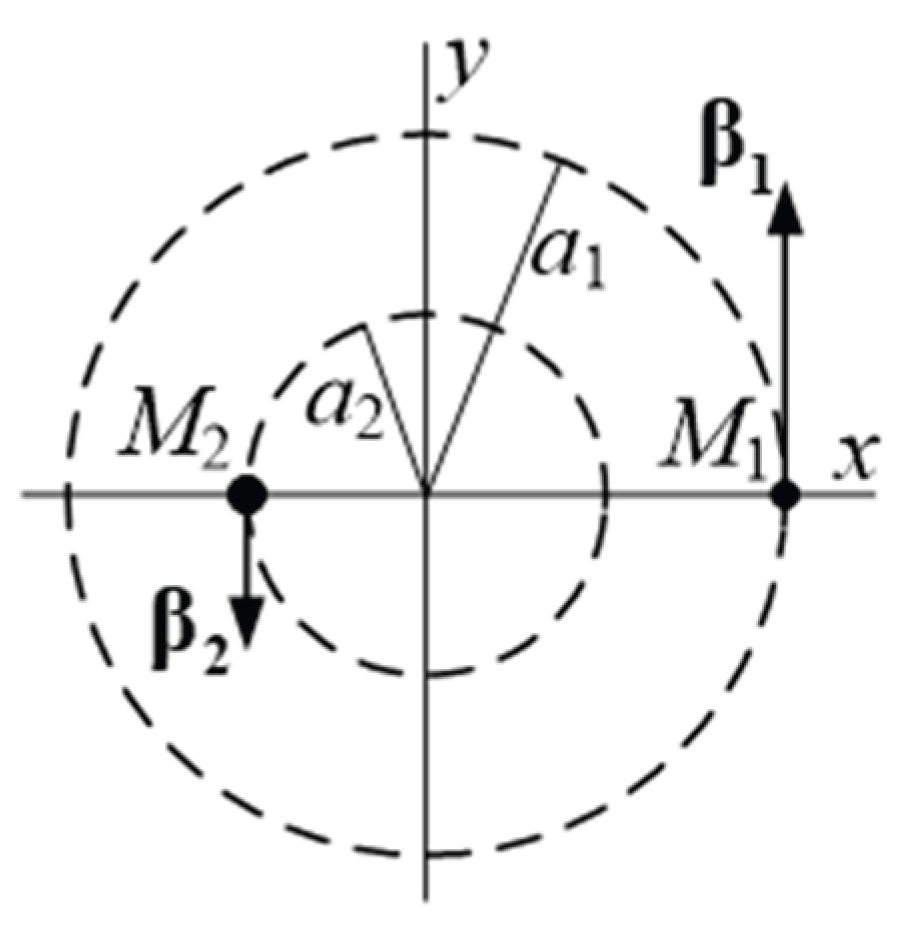
Figure 5.
Metric component vs. normalized Cartesian coordi nate in a static, homogeneous universe with a flat 3-volume for indicated values of dimensionless curvature,. Dashed curve is for .
Figure 5.
Metric component vs. normalized Cartesian coordi nate in a static, homogeneous universe with a flat 3-volume for indicated values of dimensionless curvature,. Dashed curve is for .
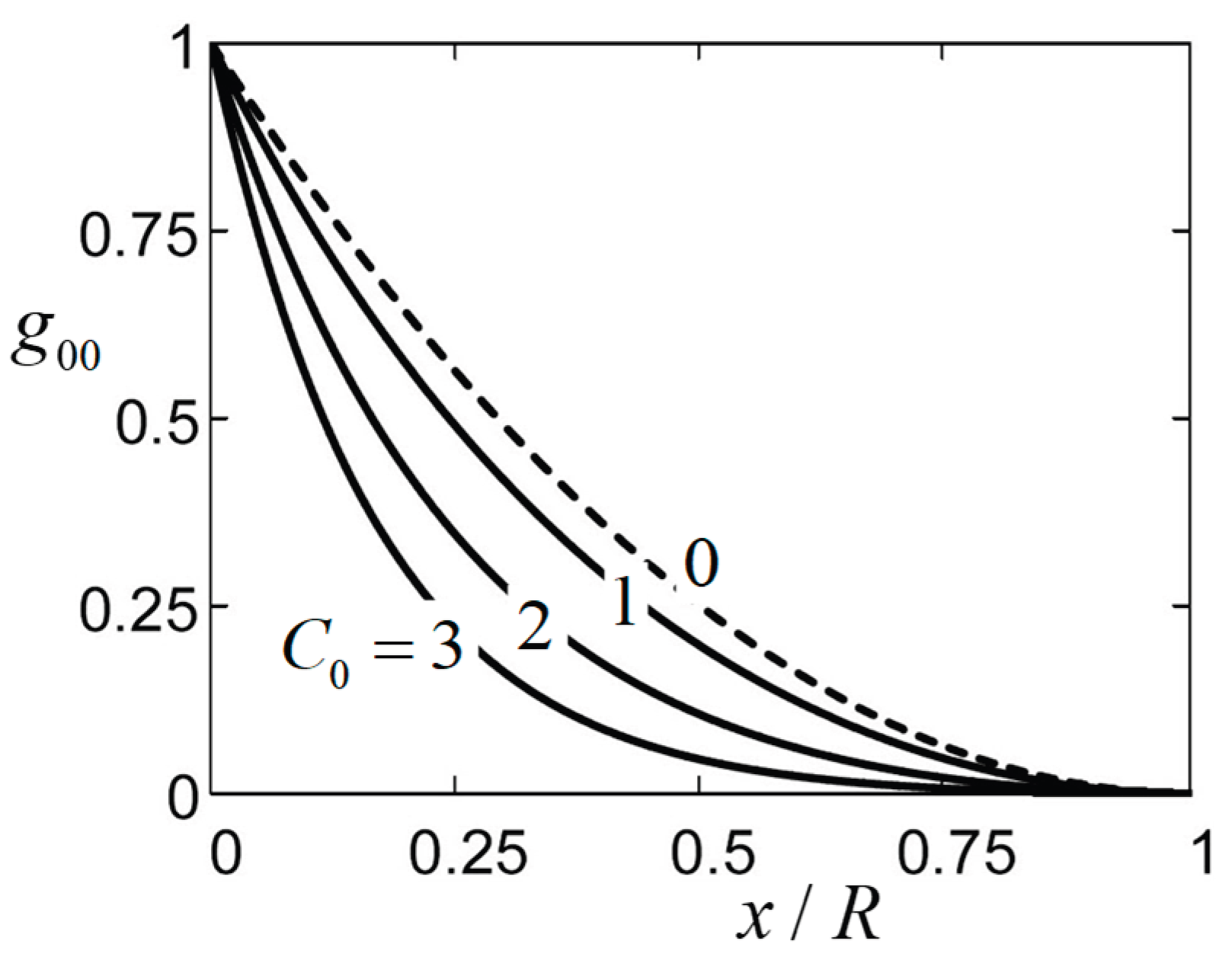
Figure 6.
Range , normalized to , in a static universe of a particle vs. its initial specific 3-momentum , normalized to , for indicated values of curvature constant .
Figure 6.
Range , normalized to , in a static universe of a particle vs. its initial specific 3-momentum , normalized to , for indicated values of curvature constant .
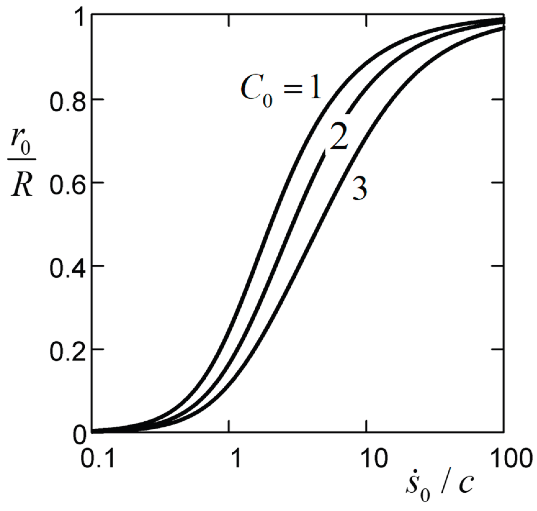
Figure 7.
A configuration for determining effects of drag arising from the CGB and time dilation. An observer at rest at the origin in watches a particle at a fixed range bouncing with elastic collisions between two walls separated by .
Figure 7.
A configuration for determining effects of drag arising from the CGB and time dilation. An observer at rest at the origin in watches a particle at a fixed range bouncing with elastic collisions between two walls separated by .
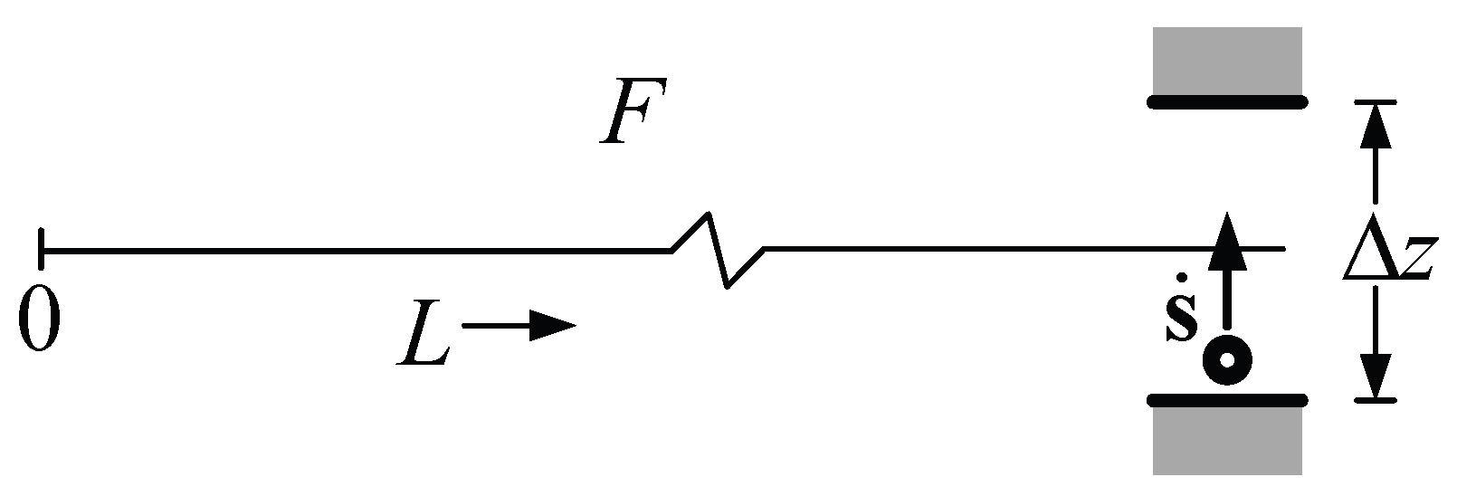
Figure 8.
Ratio of the total energy density of a static universe to the critical energy density of a ΛCDM universe vs. dimensionless curvature parameter .
Figure 8.
Ratio of the total energy density of a static universe to the critical energy density of a ΛCDM universe vs. dimensionless curvature parameter .
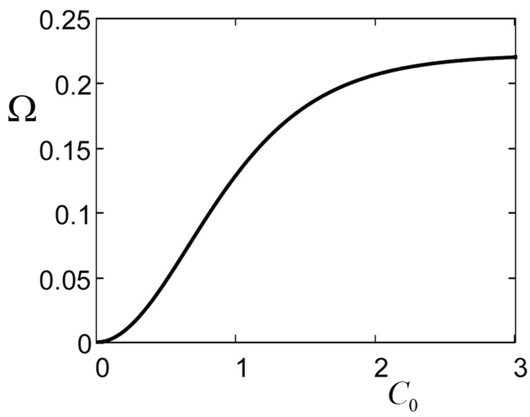
Figure 9.
Distance modulus function of SN-Ia vs. redshift parameter in a static universe for (dotted curve), (dashed curve), and (solid curve) from Eq. (81). Instrument-calibration constant was chosen for each curve to give least-squares best fit to data. Data from [56].
Figure 9.
Distance modulus function of SN-Ia vs. redshift parameter in a static universe for (dotted curve), (dashed curve), and (solid curve) from Eq. (81). Instrument-calibration constant was chosen for each curve to give least-squares best fit to data. Data from [56].
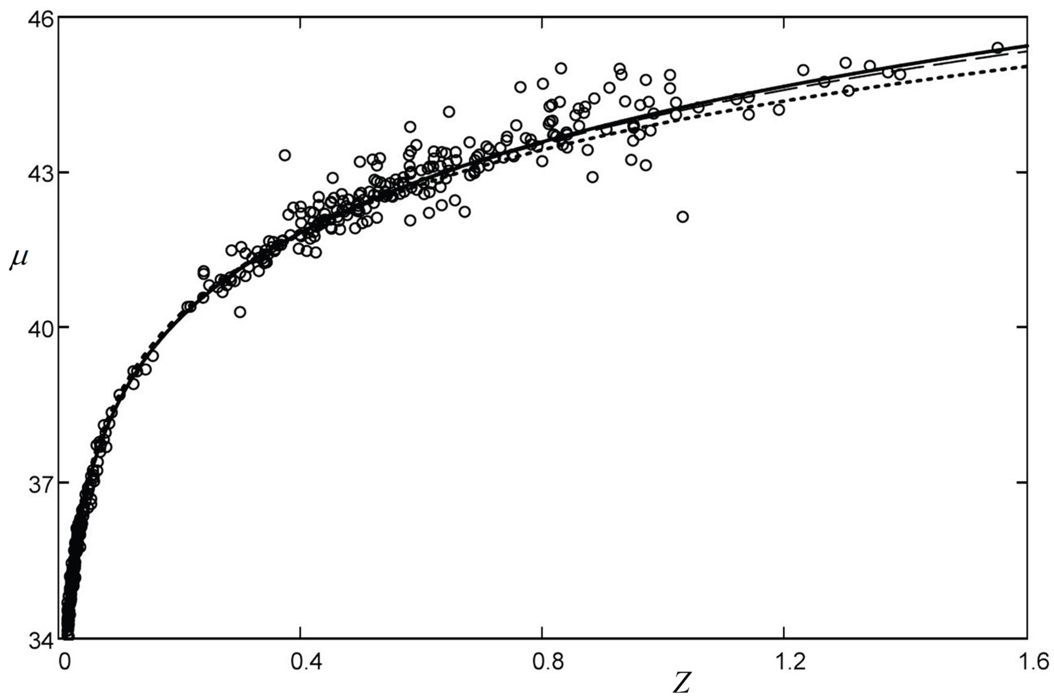
Figure 11.
Mean energy in meV of oscillator immersed in CGB at temperature 21 K. vs. normalized natural frequency in meV
Figure 11.
Mean energy in meV of oscillator immersed in CGB at temperature 21 K. vs. normalized natural frequency in meV
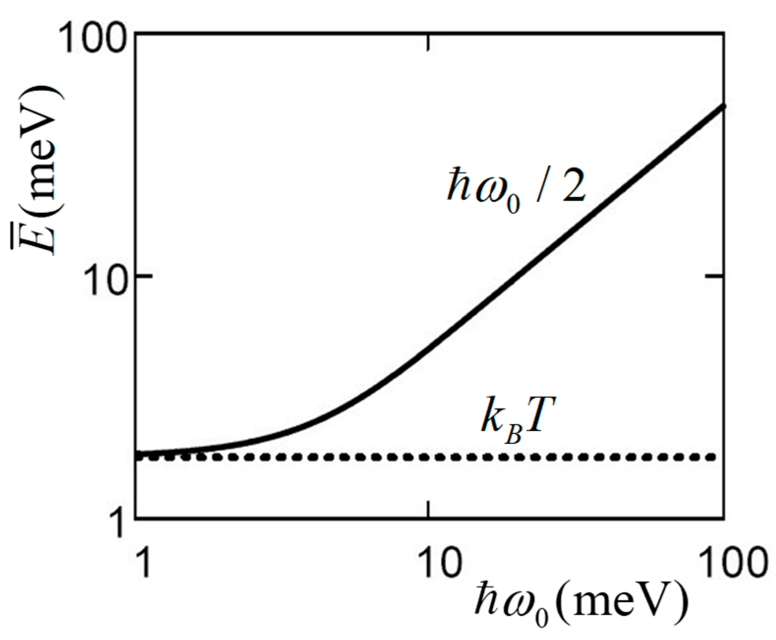
Figure 2.
(Color online) Unfiltered gravitational-wave strain vs. time (thick blue curves) of event GW150914 observed by Advanced LIGO Hanford detector, amplitude peaks indicated by circles, adapted from [36]. (a) Model of quadrupole strain waveform (thin black curves) with least-squares fit (dashed) to amplitude peaks; (b) Best fit of quadrupole-plus-dipole waveform (thin black curves), .
Figure 2.
(Color online) Unfiltered gravitational-wave strain vs. time (thick blue curves) of event GW150914 observed by Advanced LIGO Hanford detector, amplitude peaks indicated by circles, adapted from [36]. (a) Model of quadrupole strain waveform (thin black curves) with least-squares fit (dashed) to amplitude peaks; (b) Best fit of quadrupole-plus-dipole waveform (thin black curves), .
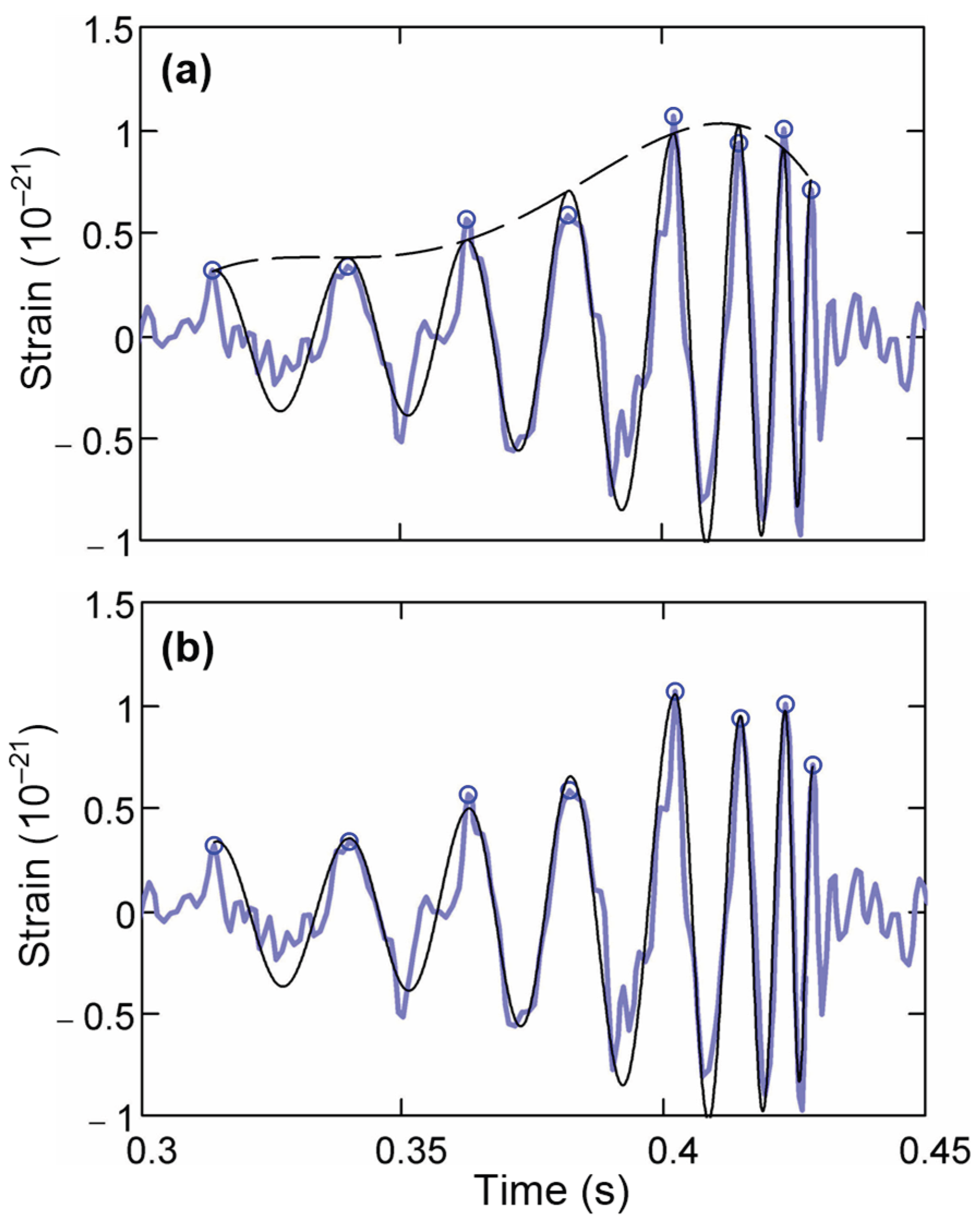
Figure 3.
Normalized variance of amplitude peaks of model waveform with unfiltered Hanford data for event GW150914 vs. ratio of model dipole-to-quadrupole strain amplitudes is a minimum for .
Figure 3.
Normalized variance of amplitude peaks of model waveform with unfiltered Hanford data for event GW150914 vs. ratio of model dipole-to-quadrupole strain amplitudes is a minimum for .
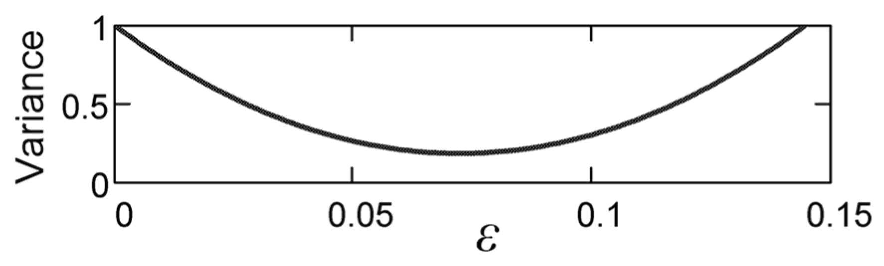
Figure 4.
(Color online) (a) Model of strain vs. time for event GW150914, quadrupole waveform (upper black curves) and dipole waveform (lower red curves) for , before filtering (dotted) and after filtering (solid). Dashed curve is envelope of peak dipole amplitude. (b) Power spectral density vs. frequency of quadrupole (upper black curve) and dipole (lower red curve) waveform models for , before filtering (dotted) and after filtering (solid).
Figure 4.
(Color online) (a) Model of strain vs. time for event GW150914, quadrupole waveform (upper black curves) and dipole waveform (lower red curves) for , before filtering (dotted) and after filtering (solid). Dashed curve is envelope of peak dipole amplitude. (b) Power spectral density vs. frequency of quadrupole (upper black curve) and dipole (lower red curve) waveform models for , before filtering (dotted) and after filtering (solid).
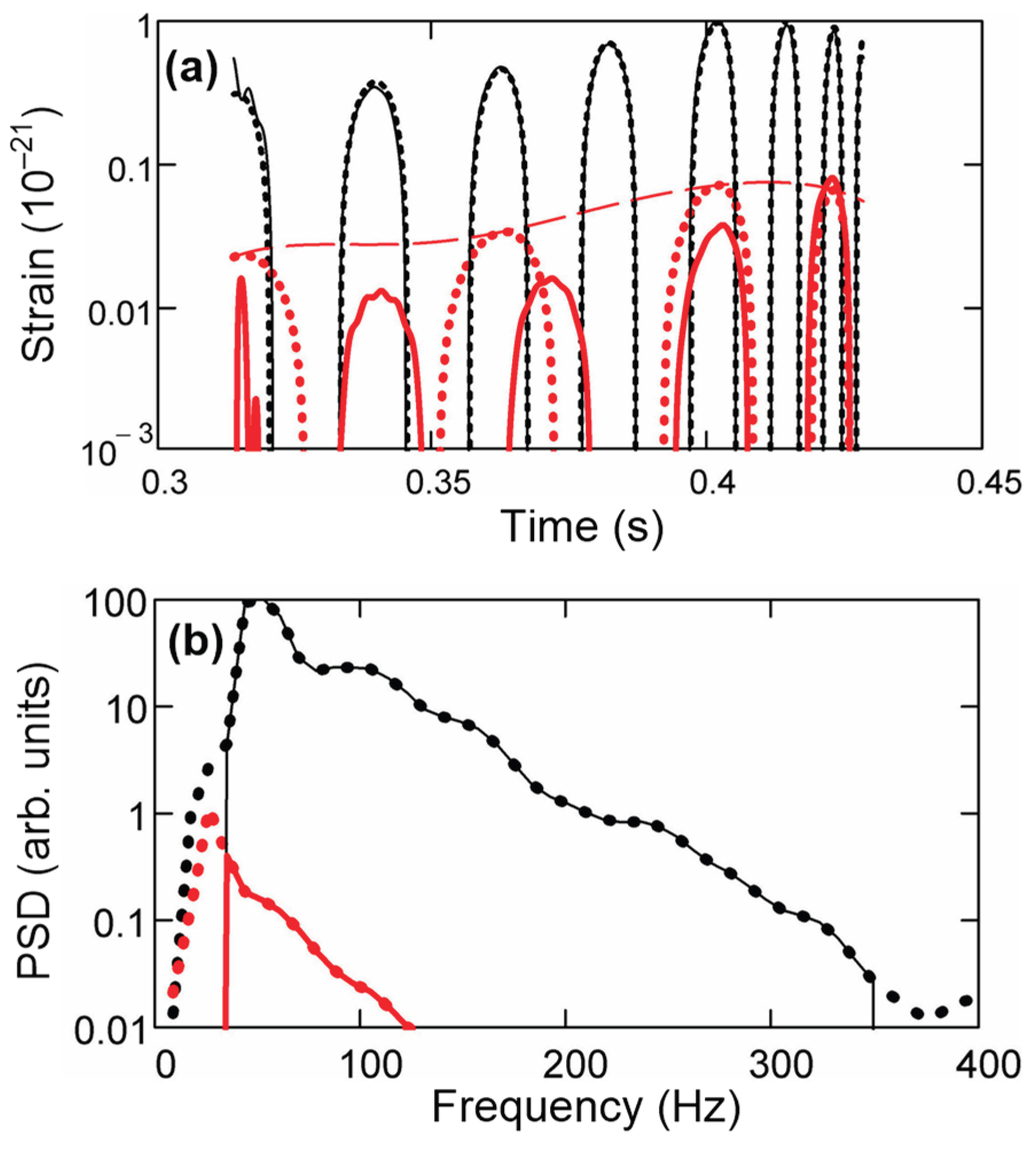
Table 1.
Correspondence between electromagnetic and weak gravitational fields and forces of a relativistic particle shows what general relativity might have looked like if it had been developed first as a vector theory, neglecting gravitation of fields.
Table 1.
Correspondence between electromagnetic and weak gravitational fields and forces of a relativistic particle shows what general relativity might have looked like if it had been developed first as a vector theory, neglecting gravitation of fields.
| Electromagnetism | Gravitation – Linear approximation |
|
|---|---|---|
| Source | ||
| Velocity 4-vector | ||
| Lorentz factor | ||
| Coupled source velocity | ||
| Current density | ||
| Conservation law | ||
| 4-vector potential | ||
| Field tensor | ||
| Lorentz/Hilbert gauge condition | ||
| Field equation in Lorentz/Hilbert gauge | ||
| Solution of field equation | ||
| Test mass | ||
| Rest mass | ||
| Velocity 4-vector | ||
| Lorentz factor | ||
| Coupled 4-velocity | ||
| Coupled momentum 3-vector | ||
| Covariant equation of motion |
||
| Force equation | ||
| Test mass at rest; transverse gauge | ||
| Force equation | ||
| Force equation, | ||
| Angular distribution of dipole power, | ||
| Total dipole power, | ||
| Scattering cross section for unpolarized radiation |
||
| Energy density of CMB/CGB |
||
Table 2.
The results in Section 2 and Section 3 of this paper are derived and supported by the appendices indicated in this table.
| Section | Subject | Appendices |
|---|---|---|
| 2.1 | Covariant vector field and force equations | A, B |
| 2.2 | Linearized 3-vector force equation | C, D |
| 3.1 | Gravitational impulse of a particle in uniform motion | E |
| 3.2 | Dipole radiation from a rotating binary | F, G, H |
| 3.3 | Dipole radiation fields, polarization, and power | I, J, K |
| 3.4 | Strain waveform model for GW150914 | L |
| 3.5 | Scattering of dipole gravitational waves | M, N |
| 3.6 | Quantization and statistics of the CGB | O |
| 3.7 | Stochastic fields of the CGB | P |
| 3.8 | Drag on particles in the CGB | Q |
| 3.9 | Exact metric of a static, homogeneous universe | R |
| 3.10 | Redshift of light in a static universe | S |
| 3.11 | Particle motion in a static universe | T |
| 3.12 | Appearance of cosmic acceleration in a static universe | U |
| 3.13 | Hubble constant, drag constant, dipole anisotropy, and CGB | V, W, X |
| 3.14 | Quantum oscillators in the CGB | Y |
Table 3.
Recent measurements of Hubble constant by several collaborations and corresponding values of the time-dilation drag constant and of the temperature of the CGB in a static, homogeneous universe.
Table 3.
Recent measurements of Hubble constant by several collaborations and corresponding values of the time-dilation drag constant and of the temperature of the CGB in a static, homogeneous universe.
| Year | Ref. | Collaboration/ Approach |
Hubble Constant, |
Drag Constant, |
Temperature of CGB, T(K) |
|---|---|---|---|---|---|
| 1999 | [58,59] | Summary | 716 | 0.690.06 | 211 |
| 2022 | [57] | Planck | 67.40.5 | 0.6550.005 | 20.30.1 |
| 2022 | [60] | SH0ES | 73.01.0 | 0.7090.010 | 21.10.2 |
| 2023 | [61] | Grav. lensing | 64.84.4 | 0.6300.042 | 19.90.7 |
| 2023 | [62] | ACT:DR6 | 68.31.1 | 0.6640.011 | 20.40.2 |
| 2023 | [63] | CATS | 72.92.0 | 0.7080.020 | 21.10.3 |
Table 4.
Recent measurements of Hubble constant by several collaborations and corresponding temperatures and energy densities of the CGB in a static, homogeneous universe, from Eqs. (88) and (89).
Table 4.
Recent measurements of Hubble constant by several collaborations and corresponding temperatures and energy densities of the CGB in a static, homogeneous universe, from Eqs. (88) and (89).
| Year | Ref. | Collaboration/ Approach |
Hubble Constant, |
Temperature of CGB, T(K) |
Energy Density, |
|---|---|---|---|---|---|
| 1999 | [58,59] | Summary | 716 | 211 | 900200 |
| 2022 | [57] | Planck | 67.40.5 | 20.30.1 | 81020 |
| 2022 | [60] | SH0ES | 73.01.0 | 21.10.2 | 94040 |
| 2023 | [61] | Grav. lensing | 64.84.4 | 19.90.7 | 740110 |
| 2023 | [62] | ACT:DR6 | 68.31.1 | 20.40.2 | 82030 |
| 2023 | [63] | CATS | 72.92.0 | 21.10.3 | 94060 |
Table 5.
Comparison of CGB properties in a static, homogeneous universe with CMB for and , so that .
Table 5.
Comparison of CGB properties in a static, homogeneous universe with CMB for and , so that .
| Property | CMB | CGB |
|---|---|---|
| Temperature, T(K) | 2.725 | |
| Mean energy density, (eV/cm3) | 0.260 | |
| Most probable wavelength, (μm) | 1060 | |
| Most probable angular frequency, (1012 s–1) | 1.77 | |
| Mean number density of bosons, (mm–3) | 0.410 | |
| Mean energy/boson, (meV) | 0.634 |
Table 7.
Benchmarks, predictions, and proposed tests of the concepts proposed in this paper.
| BENCHMARKS | PREDICTIONS | TESTS | |
|---|---|---|---|
| 1. Gravitation is a vector field | |||
| Covariant-vector linearized field and force equations identical to form of vector-field electromagnetism | See below | See below | |
| Hilbert repulsion, Eq. (14) agrees with [16] | Amplitude of repulsive impulses at LHC [15,24] | Measurement of repulsion with high-Q detector at LHC [15,24] | |
| No benchmarks for weak gravitational sources at high speeds | Gradient signal from corrugated flywheel [24] | Test of Eq. (11) with flywheel, gradiometer [24] | |
| Unbound orbits in Schwarzschild field, Eq. (11) agrees with [13,21] | Velocity field of Eq. (11) applies to unbound orbits in weak field [21] | Analytical, computational tests of Eq. (11), uniform motion [15,21] | |
| Velocity field of mass in uniform motion, Eq. (11) agrees with [14,15,21] | Velocity field of Eq. (11) applies to uniform motion in weak field [15,21] | Analytical, computational tests of Eq. (11), uniform motion [15,21] | |
| Vector-field impulse calculation gives correct deflection of light, Sec. 3.1 | Spacecraft fly-by anomalies resolved by vector-field impulse and metric time dilation, Sec. 3.1 and 3.9 | Compare fly-by anomalies with vector-field and time-dilation predictions, Secs. 3.1 and 3.9 | |
| Pioneer anomaly is anomalous acceleration of spacecraft of order towards Sun, [80,81] | Pioneer anomaly consistent with metric time dilation, Secs. 3.9, 3.11 | Compare metric time dilation with round-trip comms and other potential causes, Sec. 3.10 | |
| Dipole gravitational radiation associated with vector fields same as quadrupole radiation, Secs. 3.2, 3.3 | See “Dipole gravitational waves exist” | See “Dipole gravitational waves exist” | |
| 2. Dipole gravitational waves exist | |||
| Radiation from well-behaved binaries same for dipole waves as quadrupole waves, Secs. 3.2, 3.4 | Compact-binary mergers disrupt interference, reveal dipole waves, Sec. 3.4 | Test correlation of disruption of dipole-wave interference with existing strain data, Sec. 3.4 | |
| Stochastic motion of all particles with diffusion coefficient , Sec. 3.14 | Dipole waves apply physical forces to particles, Eq. (24) | Distinguish physical forces of dipole waves from coordinate distortions of spacetime by quadrupole waves | |
| 3. Gravitational fields are quantized by massless spin-1 bosons | |||
| Electromagnetic vector fields are quantized by massless spin-1 bosons | See “The CGB comprises spin-1 bosons obeying photon statistics” | See “The CGB comprises spin-1 bosons obeying photon statistics” | |
| 4. The CGB comprises spin-1 bosons obeying photon statistics | |||
| Vector electromagnetic field mediated by spin-1 bosons obeying photon statistics | Spin-1 gravitons of CGB have Planck distribution, Sec. 3.6 | Measure or infer properties of CGB blackbody, including temperature, Sec. 3.7 | |
| CMB, comprising spin-1 bosons obeying photon statistics, exhibits dipole anisotropy, Sec. 3.13 | CGB exhibits dipole anisotropy with respect to same local rest frame as CMB | Measure CGB dipole anisotropy by drift of particles, molecular reso-nances, other means, Secs. 3.13, 4.2 | |
| Mean energy density of CGB from Nyquist relations agrees with Stefan-Boltzmann law, Secs. 3.7, 4.2 | See above | See above | |
| 5. An Einstein static universe accounts for key cosmological observations | |||
| Static universe model accounts for Hubble redshift, appearance of cosmic acceleration, low mean density of universe | Static universe model accounts for other key cosmological observations, such as mature galaxies at high Z, Sec. 4.3 | Seek key cosmological observations for which static universe cannot account | |
| Redshift in static universe from metric time dilation satisfies minimum requirements for tired light, Secs. 3.10, 3.12, 4.3 | Some or all of Hubble redshift due to metric time dilation, not expansion of universe, Secs. 3.9, 3.10 | Direct measurement of cosmic acceleration [100] and further deep galaxy surveys like [94,95,96,97,98,99], Secs. 3.10, 3.12, 4.3 | |
| 6. The CGB underlies stochastic mechanics and theSchrödinger equation | |||
| CGB stochastic fields: Apply physical forces; are random with constant rms; act same on charged and uncharged; dominate CMB | Hubble constant proportional to , Eq. (88) | Measure CGB temperature to test proportionality, Eq. (88) | |
| Manifestations of the Schrödinger equation, zero-point and mean energy of oscillators | Minimum energy of 1D oscillator in CGB is about 1.8 meV (21 K), Sec. 3.14, Fig. 11 | Measure minimum mean energy of oscillators | |
| Diffusion coefficient for mass M in CGB appears to be , Sec. 3.14, Eq. (92) | Diffusion coefficient is | Exact calculation of effects of CGB modes with Planck distribution on Brownian motion | |
Table 6.
Some key experimental and astronomical observations relating to general relativity and the gravitational field theories necessary to explain them
Table 6.
Some key experimental and astronomical observations relating to general relativity and the gravitational field theories necessary to explain them
| Year | Ref. | Names of Observers |
Observations | Explained by Field Theory |
|---|---|---|---|---|
| 1859 | [71] | Le Verrier | Precession of Mercury’s orbit | Tensor |
| 1915 | [73] | Einstein’s final formulation of general relativity | ||
| 1919 | [74] | Eddington | Deflection of starlight during solar eclipse | Vector |
| 1960 | [53] | Pound, Rebka | Gravitational frequency shift on Earth | Scalar |
| 1982 | [41] | Taylor, Weisberg | Decay of binary orbits by radiation | Vector |
| 2015 | [36] | LIGO | Radiation from merger of black holes | Tensor |
Disclaimer/Publisher’s Note: The statements, opinions and data contained in all publications are solely those of the individual author(s) and contributor(s) and not of MDPI and/or the editor(s). MDPI and/or the editor(s) disclaim responsibility for any injury to people or property resulting from any ideas, methods, instructions or products referred to in the content. |
© 2026 by the authors. Licensee MDPI, Basel, Switzerland. This article is an open access article distributed under the terms and conditions of the Creative Commons Attribution (CC BY) license (http://creativecommons.org/licenses/by/4.0/).
Copyright: This open access article is published under a Creative Commons CC BY 4.0 license, which permit the free download, distribution, and reuse, provided that the author and preprint are cited in any reuse.


