

Submitted:
15 June 2026
Posted:
16 June 2026
You are already at the latest version
Abstract
We present a portable, cost-effective, and innovative method for experimentally verifying Ohm’s law in alternating current (AC) resistive circuits using two smartphones: one functions as a signal generator (audio output) and the other as an oscilloscope (microphone input). By connecting identical resistors in series, we systematically increase the total resistance and measure the voltage across a fixed reference resistor. Our results reveal an inverse relationship between the reference voltage and the total resistance, in agreement with Ohm’s law. Fitting the data to a power law yields an exponent of -1.004, which deviates by only 0.4% from the theoretical value of -1. The proportionality constant obtained differs by only 0.7% from the value calculated directly from the measurements. These minimal discrepancies, achieved using non-traditional, uncalibrated equipment and commercial resistors, demonstrate that our methodology is accessible, reproducible, and accurate. This approach validates Ohm’s law with high precision and underscores the potential of mobile devices as reliable experimental tools for physics education, particularly in unconventional or remote laboratory environments.
Keywords:
Ohm’s law
; series circuits
; alternating current
; signal generator
; oscilloscope
; smartphone
1. Introduction
In direct current (DC) circuits, as illustrated in Figure 1a, both the applied voltage and the current remain constant (Figure 1b). Ohm’s law, formulated by Georg Simon Ohm in 1827 [1], establishes a linear relationship between voltage and current in conductive materials that display ohmic behavior at a constant temperature. This relationship has been consistently validated in laboratory settings using commercial resistors of various values, provided that the temperature remains constant and the current does not exceed the manufacturer’s specified limits [2]. Mathematically, Ohm’s law is represented by the following formula:
where , measured in volts (V), denotes the potential difference across the resistor; is the resistance measured in ohms (Ω); and is the electric current, measured in amperes (A), which indicates the magnitude of current flowing through the circuit. Digital multimeters and regulated voltage sources are commonly employed to demonstrate the relationships among these physical quantities and to verify Eq. (1).
In alternating current circuits, such as the example illustrated in Figure 1c, both voltage and current vary as functions of time (see Figure 1d). Ohm’s law defines the relationship between voltage (V), current (I), and impedance (Z), where V, I, and Z are represented as phasors.
Impedance quantifies the total opposition to alternating current, encompassing both the circuit’s resistance and the reactance of components such as capacitors and inductors. In circuits containing only resistive elements, the impedance (Z) equals the resistance (R), so Ohm’s law in the time domain maintains the same form as in direct current circuits:
Equation (2) describes a linear, instantaneous, and phase-shift-free relationship between voltage and current, as illustrated in Figure 1d. The current through the resistor (R) mirrors the time history of the voltage applied across its terminals, accounting for the absence of phase shift. When the voltage reaches its maximum, the current also reaches its maximum; similarly, when the voltage crosses zero, regardless of the slope’s direction, the current behaves identically.
In Figure 1c, if the voltage supplied by the source exhibits no initial phase shift, the potential difference across the resistor will similarly lack an initial phase shift. Consequently, given that , the current through the resistor, which represents the circuit current, can be expressed as:
Equation (3) shows that the instantaneous current has the same time dependence as the voltage, confirming the absence of a phase shift between them. Additionally, equation (3) shows that the maximum current in the resistor is directly proportional to the maximum applied voltage, which permits Ohm’s law to be formulated using the maximum values of these variables:
In an alternating current circuit containing several resistors in series, as depicted in Figure 2, the virtual oscilloscope displays the voltage and current (gray and yellow traces, respectively) across the reference resistor. This setup enables verification of Ohm’s Law using the relationship presented in equation (4). According to equation (4), the current through the reference resistor () is 0.515 mA, which corresponds to the maximum current indicated on the virtual oscilloscope in Figure 2. The current can also be determined by dividing the maximum amplitude of the applied voltage by the total resistance of the circuit (), thereby confirming the validity of Ohm’s Law when maximum instantaneous values of voltage and current are used in purely resistive AC circuits.
Analysis of the maximum voltage across the reference resistor in the circuit shown in Figure 2 demonstrates that increasing the number of resistive components decreases the maximum current. Consequently, the maximum voltage across the reference resistor also decreases proportionally. According to Ohm’s law (equation (4)) and given that the maximum current in the circuit equals that of the reference resistor, a relationship exists between the maximum voltage across the reference resistor and the total resistance of the circuit.
The maximum reference voltage is as follows:
Equation (6) demonstrates that the maximum voltage across the reference resistor is inversely proportional to the total resistance of the AC circuit, assuming constant amplitude and frequency. This approach offers an alternative way to verify Ohm’s law in AC circuits without an AC current RMS meter by varying the circuit resistance and measuring the maximum voltage across a reference resistor.
In the past decade, mobile devices have become valuable tools for experimental work in physics and engineering. Their effectiveness stems from integrated sensors and specialized applications that support experiments in mechanics [3,4,5,6], optics [7,8,9,10], fluid mechanics [11,12,13], electricity and electronics [14,15,16], magnetism [17,18,19], and other fields.
This activity uses a purely resistive AC circuit to relate the voltage across a reference resistor to the total resistance of the circuit, thereby verifying Ohm’s law in a series resistor configuration. Following the methodology established by previous authors [15,16,20], the audio output of one smartphone serves as a signal generator, while the microphone input of another smartphone serves as an oscilloscope. The amplitude and frequency of the audio signal from the generator smartphone are kept constant while the circuit resistance is varied. The maximum amplitude detected across the reference resistor in each case is measured using the smartphone oscilloscope. Analysis of the results allows for a comparison between the experimental mathematical model relating to and and the theoretical model predicted by equation (6).
2. Method
Figure 3 presents the circuit employed to demonstrate Ohm’s law. A Samsung Galaxy A04 (SM-A045M/DS) smartphone served as the signal generator, utilizing the “Tone Generator” function of the Physics Toolbox Suite app [21]. A Xiaomi Redmi Note 7 (M1901F7E) smartphone functioned as the oscilloscope via the “Audio Scope” feature of the Phyphox app [22]. Both devices ran on the Android operating system.
Each resistor was measured individually using a SparkFun 70C digital multimeter, with the measurement uncertainty estimated based on the instrument’s technical specifications [23]. A total of ten 0.47 kΩ resistors (nominal value) were required. To connect the mobile devices to the circuit, commercial 3.5 mm male TRRS connectors were utilized. Four-wire cables were soldered to these connectors, allocating one wire per channel: left audio, right audio, microphone, and ground. Finally, alligator clips were attached to the bare ends of the wires to ensure a reliable connection to the circuit.
Because smartphones are not specifically designed as laboratory measuring instruments, the output impedance of a smartphone functioning as a signal generator is nonzero, and the input impedance when used as an oscilloscope is finite. Consequently, both values needed to be measured.
The output impedance () of the smartphone functioning as a generator is measured by applying a sinusoidal audio signal at a fixed frequency and constant amplitude. A second smartphone records the maximum no-load voltage (open-circuit voltage, ) and the maximum load voltage () when a load resistor () is connected between the audio output and the signal generator’s ground. In this configuration, the load resistor and the output impedance of the audio generator form a voltage divider, allowing the application of equation (7) to determine the generator’s output impedance. Figure 4 presents the connection diagrams for the devices and the load resistor used in this procedure.
A similar methodology was employed to determine the input impedance of the smartphone functioning as an oscilloscope (), with the modification that a known resistor was connected in series with the audio signal generator. In this configuration, the series resistance and the smartphone’s input impedance form a voltage divider, allowing the application of equation (8) to determine the unknown value.
The output impedance of the smartphone functioning as a signal generator was measured across frequencies from 0.2 kHz to 1.0 kHz, using a load resistance of 47 Ω (measured value: 45.9 Ω). Similarly, the input impedance of the smartphone operating as an oscilloscope was evaluated over the same frequency range using a reference resistance of 4.7 kΩ (experimental value: 4.59 kΩ).
For all measurements, the amplitude of the signal generator was held constant by setting the mobile device volume to level 8, starting from zero intensity [20].
The circuit depicted in Figure 3 was assembled with a single resistor (), and the signal was measured on the smartphone oscilloscope between points a and b as indicated in the diagram. In this configuration, the total circuit impedance () is determined by the series combination of the smartphone signal generator’s output impedance () and the parallel equivalent of and the smartphone oscilloscope’s input impedance ().
Resistors were sequentially added, modifying the circuit configuration as shown in Figure 3. The total resistance of the circuit was then calculated using equation (10):
where was obtained using equation (9), and the resistances , , and subsequent terms correspond to the measured values of each individual resistor.
For each configuration, the maximum voltage across the reference resistor was measured. Measurements were recorded each time the negative terminal of the audio generator was connected to positions c, d, e, f, and subsequent nodes indicated in Figure 3, while the audio output remained at position a. The data were exported in an Excel-compatible format for subsequent analysis, and screenshots were saved to document changes in the , signal as total resistance increased.
For each exported file, the voltage peaks of the sinusoidal signal were identified to calculate the average maximum voltage (V_m,ref) and its uncertainty. Subsequently, was plotted against to evaluate the empirical mathematical model against the theoretical model described in equation (6).
3. Results and Discussion
Figure 5 presents the output impedance () of the smartphone operating as a signal generator and the input impedance () of the device functioning as an oscilloscope. The experimental results demonstrate that both impedances remain constant and independent of the audio signal frequency within the analyzed range (0.20 kHz to 1.0 kHz). Furthermore, within this interval, both impedances exhibit purely resistive behavior, with no frequency-dependent variations attributable to reactive elements. This stability justifies using a single average impedance value across all calculations, thereby minimizing additional systematic errors.
Figure 6 displays screenshots obtained using the smartphone-based oscilloscope (a Xiaomi Redmi Note 7; see Figure 3) for three configurations of the total circuit resistance. In each case, the voltage signal is displayed as a function of time, as measured across the reference resistor. The signal frequency was maintained at 0.50 kHz for all measurements, with variations occurring only in amplitude.
Figure 6a, which represents the condition in which the total resistance is given by Equation (9), displays a sinusoidal signal with maximum amplitude. As the circuit’s total resistance increases, as illustrated in Figure 6b (), 6c (), and 6d () there is a clear and progressive decrease in the amplitude of . This behavior directly demonstrates Ohm’s law in the time domain, indicating that the reduction in the amplitude results from the decrease in current caused by the increased total resistance. The screenshots in Figure 6 further illustrate this trend: a greater number of resistors in series, and thus a higher , produces a signal with a reduced amplitude, qualitatively confirming the behavior predicted by Ohm’s law.
The experimental results for ten total resistance configurations in the series circuit, constructed from identical resistors with a nominal value of 0.47 kΩ ± 5% (Figure 3), are summarized in Table 1. The total resistance for each configuration was calculated using equations (9) and (10) as more resistors were added. The total resistance uncertainty () arises from the propagation of uncertainties related to and , combined with the measurement uncertainties of the individual components.
Signals were captured using the “Audio Scope” function of the Phyphox application. For each configuration, the average peak voltage (, in arbitrary units, a.u.) of the sinusoidal signal across the reference resistor was determined. The standard deviation () was used to quantify the dispersion of these amplitudes.
The results indicate a significant decrease in as increases, thereby qualitatively confirming the inverse relationship predicted by Ohm’s law. Figure 7 shows the average voltage across the reference resistor for each circuit total resistance configuration. The experimental data indicate a decreasing trend, confirming the inverse relationship between voltage and resistance, as suggested by the qualitative observations in Figure 6.
Fitting the data using a power function (orange line) yielded an expression of the form , with an exponent . This value approximates the theoretical exponent of −1, derived from Ohm’s law for a series circuit powered by a source of constant amplitude and frequency [Eq. (6)]. The relative discrepancy of 0.4% between the experimental and theoretical exponents is considerably smaller than the 10% limit commonly accepted in laboratory practices with uncalibrated instrumentation, demonstrating the precision achieved with the proposed methodology.
To verify the consistency of the proportionality constant , the theoretical model from equation (6) was evaluated. As established in the methodology, considering the parallel and series impedance combinations with the external reference resistor () in the circuit (Figure 3), the voltage measured between points a and b is . Since the equivalent resistance is 0.396 kΩ is (Table 1), the expected theoretical product is 0.272 u. a.⋅kΩ. This calculated value closely matches the fitting coefficient derived from the power-law fit in Figure 7, exhibiting a relative difference of approximately 0.7%. This consistency, combined with the accurate experimental exponent (), provides robust validation of both the theoretical model and the experimental methodology.
The results indicate that Ohm’s law can be verified with high precision using only two smartphones as signal generators, an oscilloscope, commercial resistors, and TRRS cables. The internal consistency of the experiment, demonstrated by the agreement among the fitting exponent, the proportionality constant, and the directly measured values, underscores the reliability of mobile devices as experimental physics measurement tools, particularly in unconventional laboratory settings or remote learning environments.
4. Conclusion
The experimental results confirm the validity of Ohm’s law in series resistive circuits carrying alternating current, utilizing only two smartphones as a signal generator and an oscilloscope. The voltage amplitude measured across the reference resistor decreases in inverse proportion to the circuit’s total resistance, consistent with theoretical predictions. Fitting the mathematical model to the experimental data yields a fitting exponent of –1.004, which differs from the ideal value of –1 by only 0.4%. Similarly, the proportionality constant obtained from the power-law fit closely matches the value calculated directly from the measurements, differing by 0.7%. These minimal discrepancies, observed with uncalibrated mobile devices and standard commercial resistors (±5% tolerance), support both the validity of Ohm’s law and the accuracy and reliability of the smartphone-based methodology. This approach offers a portable, economical, and reproducible alternative to conventional laboratory equipment, making it suitable for resource-limited environments, distance education, and inquiry-based learning. The results underscore the potential of everyday mobile technology as a scientific tool for verifying fundamental principles of physics.
References
- Young, H. D.; Freedman, R. A. Sears y Zemansky FÍSICA UNIVERSITARIA con Física Moderna, 13ª edición ed.; PEARSON, México, 2013; vol. 2, pp. 822–825. [Google Scholar]
- Gomasang, P.; Tanarom, J. A Study of Thermal Effect on High-Current Standard Resistor. IEEE, 20th International Conference on Electrical Engineering/Electronics, Computer, Telecommunications and Information Technology (ECTI-CON), May 2023; pp. pp. 1–4. [Google Scholar] [CrossRef]
- Kaps, A.; Splith, T.; Stallmach, F. Implementation of smartphone-based experimental exercises for physics courses at universities. Phys. Educ. 2021, vol. 56(no. 3), 035004. [Google Scholar] [CrossRef]
- Anni, M. Quantitative Comparison between the Smartphone Based Experiments for the Gravity Acceleration Measurement at Home. Educ. Sci. 2021, vol. 11(no. 9), 493. [Google Scholar] [CrossRef]
- M. Santamaría, L.; Cruz de Gracia, E. S.; Dorneles, L. S. Kinematics in One Dimension—A Smartphone Approach. Phys. Teach. 2023, vol. 61(no. 7), 594–598. [Google Scholar] [CrossRef]
- Coramik, M.; İnanç, B. A physical pendulum experiment with Lego, Phyphox and Tracker. Phys. Educ. 2023, vol. 58(no. 5). [Google Scholar] [CrossRef]
- Gallitto, A. A.; Sancataldo, G.; Battaglia, O. R.; Fazio, C. A Low-Cost Smartphone Polarimeter and Malus’s Law. Phys. Teach. 2024, vol. 62(no. 8), 653–655. [Google Scholar] [CrossRef]
- Organtini, G. Interference of Two Point Sources Using Smartphones. Phys. Teach. 2021, vol. 59(no. 9), 709–711. [Google Scholar] [CrossRef]
- Onorato, P.; Rosi, T.; Tufino, E.; Caprara, C.; Malgieri, M. Using smartphone cameras and ambient light sensors in distance learning: the attenuation law as experimental determination of gamma correction. Phys. Educ. 2021, vol. 56(no. 4), 045007. [Google Scholar] [CrossRef]
- Rath, G. Elementary optics lab with smartphones and instant messaging. J. Phys. Conf. Ser. 2018, vol. 1076(no. 1), 012012. [Google Scholar] [CrossRef]
- Büyükdede, M. Leveraging smartphone barometric sensors for authentic physics learning: an in-flight experiment. Phys. Educ. 2025, vol. 60(no. 5), 055018. [Google Scholar] [CrossRef]
- Grant, G.; Shastri, A. Using a Smartphone Barometer to Measure the Excess Pressure of a Soap Bubble. Phys. Teach. 2025, vol. 63(no. 4), 243–245. [Google Scholar] [CrossRef]
- Salinas; Muñoz-Pérez, F. M.; Castro-Palacio, J. C.; Monsoriu, J. A. Barometric characterization of a draining container. Phys. Educ. 2023, vol. 58(no. 5), 055017. [Google Scholar] [CrossRef]
- Hurtado-Gutiérrez, R.; Tejero, Á. Measuring capacitor charge and discharge using an LED and a smartphone. Eur. J. Phys. 2023, vol. 44(no. 6), 065201. [Google Scholar] [CrossRef]
- Torriente-García; Muñoz-Pérez, F. M.; Martí, A. C.; Monteiro, M.; Castro-Palacio, J. C.; Monsoriu, J. A. Experimenting with RC and RL series circuits using smartphones as signal generators and oscilloscopes. Rev. Bras. De Ensino De Física 2023, vol. 45. [Google Scholar]
- M. Santamaría, L.; Cruz de Gracia, E. S.; Dorneles, L. S.; Correa, N. Frequency effect on reactance in RC and RL circuits—a smartphone approach. Phys. Educ. 2025, vol. 60(no. 3), 035033. [Google Scholar] [CrossRef]
- Ogawara, Y.; Bhari, S.; Mahrley, S. Observation of the magnetic field using a smartphone. Phys. Teach. 2017, vol. 55(no. 3), 184–185. [Google Scholar] [CrossRef]
- Taspika, M.; Nuraeni, L.; Suhendra, D.; Iskandar, F. Using a smartphone’s magnetic sensor in a low-cost experiment to study the magnetic field due to Helmholtz and anti-Helmholtz coil. Phys. Educ. 2019, vol. 54(no. 1), 015023. [Google Scholar]
- Westermann, N.; Staacks, S.; Heinke, H.; Möhrke, P. Measuring the magnetic field of a low frequency LC-circuit with phyphox. Phys. Educ. 2022, vol. 57(no. 6), 065024. [Google Scholar] [CrossRef]
- Torriente-García; Martí, A. C.; Monteiro, M.; Stari, C.; Castro-Palacio, J. C.; Monsoriu, J. A. RLC series circuit made simple and portable with smartphones. Phys. Educ. 2023, vol. 59(no. 1), 015016. [Google Scholar] [CrossRef]
- Vieyra Software,, “Physics Toolbox,” 2025. Available online: https://www.vieyrasoftware.net/ (accessed on 23 March 2026).
- University, RWTH Aachen, Phyphox. Available online: https://phyphox.org/ (accessed on 23 March 2026).
- sigrok. 4 July 2017. Available online: https://sigrok.org/wiki/SparkFun_70C (accessed on 28th March 2026).
Figure 1.
(a) Direct current circuit. (b) Time behavior of the voltage signal and current signal in a DC circuit. (c) Alternating current (AC) circuit. (d) In-phase sinusoidal voltage and current signals for a 2 kΩ resistor. In both DC and AC regimes, Ohm’s Law () holds in the time domain for ohmic resistors at constant temperature.
Figure 1.
(a) Direct current circuit. (b) Time behavior of the voltage signal and current signal in a DC circuit. (c) Alternating current (AC) circuit. (d) In-phase sinusoidal voltage and current signals for a 2 kΩ resistor. In both DC and AC regimes, Ohm’s Law () holds in the time domain for ohmic resistors at constant temperature.
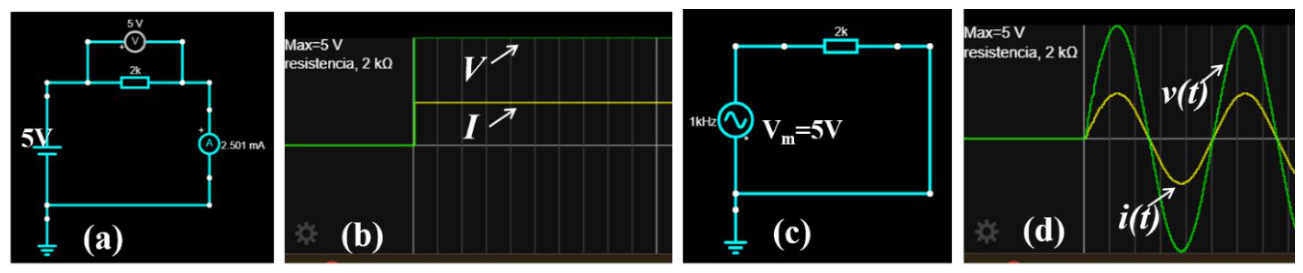
Figure 2.
The voltage (gray line) and current (yellow line) signals were displayed using a virtual oscilloscope connected to a reference resistor in an alternating current (AC) circuit with resistors in series. The observed maximum current closely matched the calculated value, thereby providing experimental confirmation of Ohm’s Law in a resistive AC circuit.
Figure 2.
The voltage (gray line) and current (yellow line) signals were displayed using a virtual oscilloscope connected to a reference resistor in an alternating current (AC) circuit with resistors in series. The observed maximum current closely matched the calculated value, thereby providing experimental confirmation of Ohm’s Law in a resistive AC circuit.
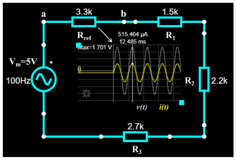
Figure 3.
(a) Schematic diagram of the circuit. The generator smartphone delivers a 1 kHz sine wave through the audio output (TRRS connector). The oscilloscope smartphone records the voltage across the reference resistor Rref using the microphone input. (b) Photographs of the experimental setup and components.
Figure 3.
(a) Schematic diagram of the circuit. The generator smartphone delivers a 1 kHz sine wave through the audio output (TRRS connector). The oscilloscope smartphone records the voltage across the reference resistor Rref using the microphone input. (b) Photographs of the experimental setup and components.
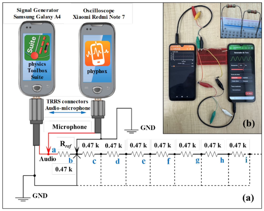
Figure 4.
Circuits employed to determine the output impedance of the smartphone generator: (a) Without a load resistor connected to the output, the maximum open-circuit voltage () is measured. (b) With a load resistor connected to the generator output, the maximum voltage under load () is measured.
Figure 4.
Circuits employed to determine the output impedance of the smartphone generator: (a) Without a load resistor connected to the output, the maximum open-circuit voltage () is measured. (b) With a load resistor connected to the generator output, the maximum voltage under load () is measured.
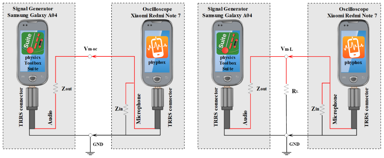
Figure 5.
Output impedance, (a), and input impedance, (b), are presented as functions of frequency for the smartphone configured as a generator and an oscilloscope, respectively. Each graph displays the average measured impedance and its associated uncertainty.
Figure 5.
Output impedance, (a), and input impedance, (b), are presented as functions of frequency for the smartphone configured as a generator and an oscilloscope, respectively. Each graph displays the average measured impedance and its associated uncertainty.
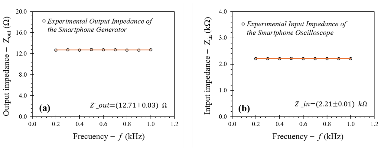
Figure 6.
Experimental screenshots of the voltage signal measured across the reference resistor indicated in Figure 3 for various total circuit resistance configurations: (a) , (b) , (c) . The signal amplitude decreases progressively as Rt increases, with the frequency held constant at 0.50 kHz across all cases.
Figure 6.
Experimental screenshots of the voltage signal measured across the reference resistor indicated in Figure 3 for various total circuit resistance configurations: (a) , (b) , (c) . The signal amplitude decreases progressively as Rt increases, with the frequency held constant at 0.50 kHz across all cases.
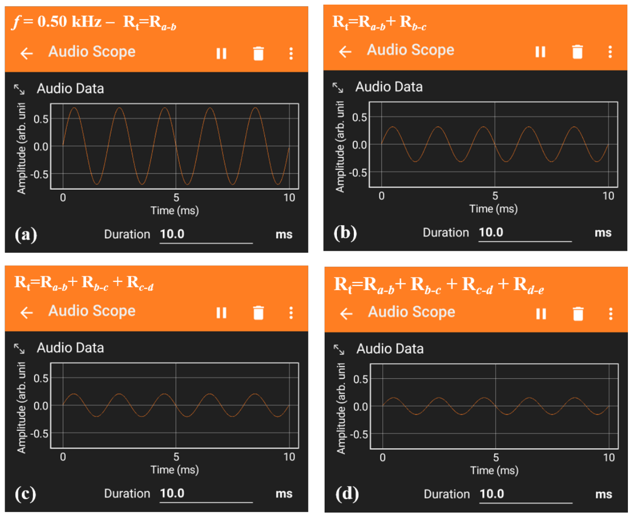
Figure 7.
Average voltage across the reference resistor () as a function of the total circuit resistance (). Circles indicate experimental data points from Table 1. The Orange line depicts the power-law fit (), yielding an exponent and coefficient .
Figure 7.
Average voltage across the reference resistor () as a function of the total circuit resistance (). Circles indicate experimental data points from Table 1. The Orange line depicts the power-law fit (), yielding an exponent and coefficient .
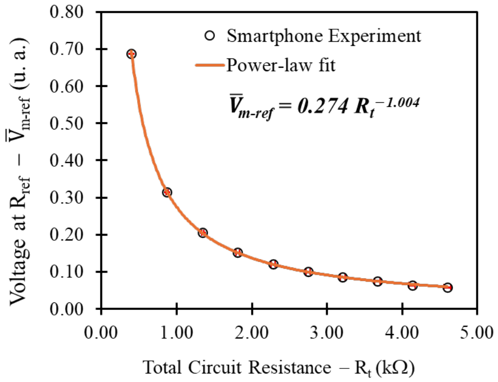

Table 1.
Measured total resistance (), average voltage peak across the reference resistor (), and their respective uncertainties (, ) for ten series circuit configurations.
Table 1.
Measured total resistance (), average voltage peak across the reference resistor (), and their respective uncertainties (, ) for ten series circuit configurations.
| 0.396 | 0.68683 | 0.007 | 0.00039 | |
| 0.871 | 0.31426 | 0.012 | 0.00020 | |
| 1.344 | 0.20544 | 0.016 | 0.00012 | |
| 1.810 | 0.15195 | 0.020 | 0.00012 | |
| 2.282 | 0.12082 | 0.024 | 0.00009 | |
| 2.744 | 0.10050 | 0.029 | 0.00008 | |
| 3.206 | 0.08613 | 0.033 | 0.00013 | |
| 3.670 | 0.07499 | 0.037 | 0.00005 | |
| 4.130 | 0.06352 | 0.041 | 0.00009 | |
| 4.603 | 0.05902 | 0.045 | 0.00003 |
Disclaimer/Publisher’s Note: The statements, opinions and data contained in all publications are solely those of the individual author(s) and contributor(s) and not of MDPI and/or the editor(s). MDPI and/or the editor(s) disclaim responsibility for any injury to people or property resulting from any ideas, methods, instructions or products referred to in the content. |
© 2026 by the authors. Licensee MDPI, Basel, Switzerland. This article is an open access article distributed under the terms and conditions of the Creative Commons Attribution (CC BY) license (http://creativecommons.org/licenses/by/4.0/).
Copyright: This open access article is published under a Creative Commons CC BY 4.0 license, which permit the free download, distribution, and reuse, provided that the author and preprint are cited in any reuse.


