Submitted:
04 June 2026
Posted:
04 June 2026
You are already at the latest version
Abstract
To promote coal purification, this study investigates the optimization and control of the downstream processes in coal gasification: the sour water gas shift reaction (SWGSR) and sour gas removal (AGR). For steady-state design, an SWGSR/AGR process model was developed using Aspen Plus software, and the simulation results were validated using data from the National Energy Laboratory. Three different process flow schemes were considered in the study. Based on the results of sensitivity analysis, the optimization variables for these processes included: steam injection flow rate, number of H₂S absorber trays, number of degassing tower trays, degassing tower feed stage, and degassing tower feed tray temperature. All of the above variables had a significant impact on the total annual cost (TAC) of each process flow scheme. The SWGSR/AGR process was designed to minimize TAC while maintaining product specifications. The TACs for Process Schemes 1, 2, and 3 were $98,967,790.9, $116,881,378.3, and $95,338,636.5, respectively. Regarding dynamic control, control structures for flow structures 1 and 3 (FS1 & FS3) are proposed. The automatic tuning method, detuning method, and Tyrens-Luyben tuning rule method are employed to determine controller parameters. Simulation results show that, under varying throughput and load disturbances, FS3 achieves faster disturbance rejection rates and setpoint tracking.
Keywords:
optimization
; control
; acid gas removal
; coal gasification
1. Introduction
As global population rapidly increases, energy demand also rapidly increases. Pulverized coal combustion plants have been widely studied to use in power generation due to abundant carbon resources (e.g., coal, biomass etc.). However, it drives air pollution higher and produces CO2 emission problems which cause climate change. Having this in mind, the researchers focused on clean coal technology which includes sulfur removal and CO2 capture, i.e., Integrated Gasification Combined Cycle (IGCC) or, coal to chemicals[1,2,3,4,5,6].
National Energy Technology Laboratory (NETL, 2007)[7] has reported that a gasification plant with CO2 capture increased its total plant annual cost by 14.41 % and the net plant efficiency (HHV basis) reduced from 38.2% to 32.5% compared to a plant without CO2 capture[7]. Therefore, how to reduce the investment and energy cost of clean coal technology is a key issue for commercialization.
Rezani et al. (2009)[8] made a comparison between different acid gas removal methods and the result shows the physical absorption method is a cost attractive process for IGCC processes. From literature survey, several physical absorption (SWGSR/AGR) process flowsheets were proposed and can be classified into five types. (1) Kohl and Nielsen (1997)9 : SWGSR first, then H2S and CO2 removal by SELEXOL solvents consecutively. (2) Robinson and Luyben (2010)[10] proposed: H2S removal first, then WGSR, finally CO2 capture. (3) Padurean et al. (2012)[11] proposed: SWGSR first, then H2S is absorbed into the bypass CO2-SELEXOL solvent from the CO2 absorber bottom stream. The SELEXOL solvent from the H2S stripper bottom stream is recycled to the CO2 absorber. (4) Bhattacharyya et al. (2011)[12] and Field and Brasington (2011)[13] proposed: SWGSR first, then H2S removal by SELEXOL solvents and the stripper with N2 (syngas) is used to recycle syngas back to the H2S absorber. Finally CO2 capture. (5) Guillermo Ordorica-Garcia et al. (2006)[14] proposed: SWGSR first, then H2S and CO2 are captured together by using SELEXOL solvents. All of them provided different kinds of design flowsheets in order to remove acid gas from coal gasification outlets. However, few papers summarized which flowsheet is economically optimal for acid gas removal processes. In the dynamic control field, Robinson and Luyben (2010)[10] provided a control scheme for IGCC processes. However, few papers have studied dynamics and control issues of these process flowsheets.
In this work, optimal design and control of SWGSR/AGR processes are investigated. In section 2, Aspen Plus Software was used to build the model and validated with NETL data. In section 3, each process was optimized to determine the minimum total annual cost (TAC). In section 4, the control structure was designed to test the control performance and operability range for FS1 and FS3.
2. Processes
In this section, design process flowsheet sequences and optimal design of coal gasification downstream processes (SWGSR/AGR) were investigated. Illinois No. 6 bituminous powders (71.7% C, 5.6%H2, 1.4%N2, 2.8%S, 0.3%Cl, 7.7%O, 10.9% ash; LHV:29.544 KJ/Kg) and 99 % O2 were fed into a Siemens gasifier to generate raw syngas[15]. The high temperature of raw syngas with carbon particles was cooled via radiant syngas cooler and water quench units. The composition and flowrate of the outlet stream were obtained by NETL[15] and are shown in Figure 1. In order to convert syngas to methane, coal gasification downstream processes have to be designed to satisfy the following specifications:
(1) the H2/CO ratio of SWGS reactor effluent stream must be set to 3:1 (for methanation reaction). (2) 99.9% of COS effluent from gasification must be converted to H2S in the COS reactor and H2S removal percentage in the H2S removal process should be 99.5 % (to prevent catalysts poisoning in the methanation processes and to comply with emission regulations). (3) CO2 capture percentage in the CO2 capture process should be 90.14 % (for CO2 emission reduction).
2.1. Process Descriptions
From literature survey, process flowsheets of coal gasification downstream processes for producing methane can be classified into three types[9,10,11]. Each process flowsheet will be discussed in the later section.
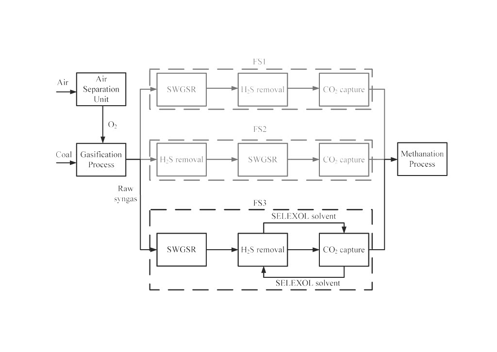
2.1.1. Process Flowsheet 1 (FS1)
The first process configuration is shown in Figure 1a namely, FS1[9]. In this flowsheet, syngas from the gasifier outlet was sent to SWGS reactor in order to (1) adjust the composition H2/CO ratio to 3:1 for methanation processes, (2) convert COS to H2S for further H2S capture purposes. SWGS and COS hydrolysis reactions in the SWGS reactor are shown as follows[16,17]:
CO + H2O ↔ CO2 + H2
COS + H2O → H2S + H2
The SWGS reactor outlet stream was cooled and pumped into a knockout drum which removes excess water and sequentially mixed with a tail gas from clean up unit before it enters the H2S absorber. Then, the H2S of the syngas from the SWGS reactor was physically absorbed by lean-SELEXOL solvent in a counter-current H2S absorber (A-1). The effluent syngas from the top of the H2S absorber was sent to the CO2 capture sub-process. The H2S-rich SELEXOL solvent from the bottom of the H2S absorber was preheated and sent to a flash tank (F-1). The operating temperature and pressure of the flash tank were used as design variables to adjust the H2S concentration at the stripper top outlet to 39.2 %. The vapor effluent stream of the flash tank was recycled back to the absorber. The liquid stream of the flash tank was then sent to the H2S stripper. The stripper distillate was cooled to 110 oF by a partial condenser to ensure most of the water condensed. The H2S was separated from syngas and sent to Claus process for further refining of the sulfur component. Loss of water and SELEXOL from the process outlet, is made-up from the reflux drum and the bottom holdup of the H2S stripper. The reboiler duty was used to maintain bottom H2S purity at 10 ppm. The lean SELEXOL solvent from the bottom of the stripper was recycled back to the top stage of the absorber at 87 oF.
The CO2 of the syngas was sequentially removed in a CO2 counter-current absorber (A-2) with a lean SELEXOL solvent after the H2S removal process. The CO2-rich SELEXOL stream was sent to three flash tanks in series to separate CO2 and SELEXOL solvent. The pressures in each flash tank are 333.91, 29.40, 2.90 psia, respectively. The first flash tank pressure was used to adjust the syngas recovery rate (SRR) to 0.9933 (SRR=AGR outlet syngas flowrate/AGR inlet syngas flowrate). The treated syngas from the top of the CO2 absorber was fed into a methanation process.
2.1.2. Process Flowsheet 2 (FS2)
The second process configuration is shown in Figure 1b namely, FS2[10]. The sequence of FS2 is: the syngas from the gasifier is sent to COS hydrolysis reactor, H2S is sequentially removed, trace of H2S is captured in a ZnO adsorption bed, then CO is converted in a water gas shift (WGS) reactor and finally CO2 is captured. The purpose of this design flowsheet is to remove sulfide components first. Then, the relatively cheaper catalysts can be used in WGS reactor.
2.1.3. Process Flowsheet3 (FS3)
The third process configuration is shown in Figure 1c namely, FS3[11]. All the units of FS1 and FS3 are the same, except the SELEXOL solvent recycle loop. In the FS3, the syngas effluent from the SWGS reactor was fed to the H2S-absorber (A-1) and H2S was absorbed into the bypass CO2-SELEXOL solvent from the CO2 absorber bottom stream. The SELEXOL from the H2S stripper bottom was recycled to CO2 absorber (A-2).
2.2. Modeling
SWGSR and AGR units were simulated by using Aspen Plus software. The thermodynamic models of SWGS/COS reactor and AGR processes were Peng-Robinson and Perturbed-Chain Statistical Associating Fluid (PC-SAFT) property method which were used to describe the gas-liquid phase behavior. The composition of physical absorption solvent (SELEXOL or DEPG) consisted of a mixture of dimethyl ether and polyethylene glycol and its chemical formula is CH3O(C2H4O)xCH3 where x can be between 3 to 9. x was set an average 5.3 which was regressed from SELEXOL vapor-liquid equilibrium data by Aspen Tech.[18]. The solubility of H2S in the SELEXOL solvent was higher than that of CO2 [19].
For FS1, the rate laws of COS and SWGS reaction over Co/Mo catalysts are shown as follows [16,17]:
where kCOS denotes rate constant of COS hydrolysis reaction (lb-mol lb-cat-1hr-1psia-1). KCOS represents equilibrium constant of COS hydrolysis reaction (psia-1). PCOS and PH2O are partial pressures of COS and H2O (psia). T is operating temperature (oF).
where kSWGS denotes rate constant of SWGS hydrolysis reaction (lb-mol lb-cat-1hr-1psia-0.84). KSWGS represents equilibrium constant of SWGS hydrolysis reaction (psia-0.86). PCO, PH2O, PH2 and PCO2 are partial pressures of CO, H2O, H2 and CO2 (psia).
COS/ SWGS reactor module was R-plug. According to NETL design, COS and SWGS reactors were designed in a parallel manner in order to completely convert COS. The feed molar flowrate ratio of COS and SWGS reactors was 0.1496:1.
Absorber/ stripper module was RadFrac. The detail settings of absorbers and strippers are shown as follows. Tray type of the absorber/ stripper was a sieve tray with a tray spacing of 2 feet. There were two tray liquid passes and the pressure drop between each tray was set at 0.5 psia. The construction materials in the H2S removal and CO2 capture sub-processes were stainless steel and carbon steel. The SELEXOL solution in AGR processes was 50 % SELEXOL, 50 % water[10]. Heat exchanger type was HeatX. The pressure drops in the cold and hot side of the heat exchanger were 10 and 20 psia. Overall heat transfer coefficient was 150 Btu hr-1ft-2 oF-1[10].
2.3. Model Simulation and Validation
The syngas composition of SWGS reactor feed was obtained from NETL[15]. The sizes of R-COS/R-WGS reactors were determined by using Aspen Plus Successive Quadratic Programming (SQP) toolbox with the following constrains (1) H2/CO ratio outlet is set to 3:1, (2) the reactor outlet temperature is lower than 957.6 oF, (3) the aspect ratio (reactor length to diameter) is set at 10.
In the H2S removal sub-process, number of absorber trays, pressure of the absorber, feed tray no., feed tray temperature, number of stripper trays and pressure of the stripper are 58, 460 psia, 7, 10, 357 oF, and 22.05 psia. In the CO2 capture sub-process, number of trays and pressure of the absorber are 10 and 444 psia. Under these simulation setting and process specifications, the base case simulation results of SWGSR outlet, top stream of H2S stripper and syngas outlet from CO2 absorber fit well with NETL data for each process flowsheet.
3. Steady-State Design: Optimization
Having introduced three process flowsheets, the objective of this work is to determine which process flowsheet is the best design structure. In the steady state design, each process was optimized to determine the minimum TAC. Then, the lowest TAC process flowsheet can be obtained. The dynamic control performance will be discussed to access the control performance of each process in a later section.
3.1. Sensitivity Analysis
In order to access which variable dominated TAC of these processes, the sensitivity analysis was made for (1) steam injection flowrate (Fsteam) in SWGS reactor inlet, (2) number of H2S absorber trays (NA-1), (3) H2S absorber pressure (PA-1), (4) number of H2S stripper trays (NS), (5) H2S stripper pressure (PS), (6) H2S stripper feed tray no. (NF), (7) H2S stripper feed tray temperature (TF), (8) number of CO2 absorber trays (NA-2), (9) CO2 absorber pressure (PA-2).The simulation results are shown in Figure 2. The triangular points in the figures denote base case design. From the results, some of these undetermined variables can be fixed due to the following reasons:
(1) PA-1 and PA-2 were operated at maximum pressure (460 psia and 444 psia). High pressure was preferred for physical absorption. This resulted in a lower TAC in this operating condition (shown in Figure 2).
(2) NS and NA-2 were set at minimum number of trays (10). A lower value of NS (or NA-2) caused lower TAC. The results were proven in Figure 2. Fewer than 10 trays is unreasonable and not considered [10].
After fixing PA-1, PA-2, NS and NA-2, five undetermined variables were used as our optimization variables.
3.2. Objective Function
The objective function of SWGSR/AGR processes is TAC. TAC includes capital cost divided by payback years plus operating cost. The payback year was set at 3 in this study. The cost functions for the various pieces of equipment in the SWGSR/AGR process and the utility cost function are based on Douglas (1988) [20] and Seider et al. (2011) [21].
3.3. Optimization
The optimization of these three flowsheets was achieved. The mathematical formulation is shown as follows:
The optimization variables are Fsteam, NA-1, PS, TF, and NF. The constraints of this process were: process specifications (H2/CO ratio, H2S recovery percentage, CO2 recovery percentage), equipment constraints (L/D, NS, NA-2), operating constraints (TR,out, PA-1, PA-2).
In order to solve the Eq. (5), the sequential searching of each optimization variable was performed to find the optimal TAC.
Using FS1 as an example to demonstrate the optimization procedure:
In FS1, the value of Fsteam in the SWGS reactor feed was given to find out corresponding TAC of the SWGS reactor sub-process. The result is shown in Figure 3 (a). The larger additional steam injection; the higher TAC requirement. The optimal TAC was located when Fsteam = 25982.4 lbmol hr-1 and was $20,108,456.6. In this design case, this process was not operable when load disturbance or throughput changed. Therefore, to attain an additional 15 % throughput change operability range, the steam injection flowrate was 32478.0 lbmol hr-1. The TAC of the modified design SWGSR sub-process increased to $25,049,655.7. After determining the optimal design of the SWGSR sub-process, the following H2S removal and CO2 capture (called acid gas removal, AGR) sub-process can then be performed to optimization. In the AGR sub-process, there are four optimization variables. The optimization flow diagram which is shown in Figure 4 was used to sequentially determine the minimum TAC. The optimization procedure is shown as below. For given AGR sub-process specifications: H2S recovery percentage (99.5 %), top stream H2S concentration of the stripper (39.2 %), bottom stream H2S concentration of the stripper (10 ppm), CO2 recovery percentage (90.14 %) and SRR (0.993), initial trial of NA-1, PS, and NF were set at 60, 22.05 psia, and 6. The minimum TAC was located at TF=368 oF found by searching in TF (the loop 1 in Figure 4) from 363 to 373 oF. The result is shown in Figure 3e. After finishing the TF search, the loop 2 NF (Figure 4) was searched from 6 to 8. The minimum TAC was located at NF =7 and TF =368 oF. Again, the optimal results of the loop 3 PS which was searched from 19.7 to 29.4 psia are shown in Figure 3 (d), (e), and (f). Finally, the optimal result of the loop 4 NA-1 which was searched from 55 to 65 was confirmed and validated with the original trial value of 60. The minimum TAC of the AGR sub-process was $ 73,918,135.2 with corresponding design variables of NA-1,= 60, PS = 22.05 psia, NF = 7, TF = 368 oF. The TACs of H2S removal and CO2 capture sub-processes were $47,446,951.3 and $ 26,471,184, respectively.
3.4. Result and Discussion
After performing the optimization of each process flowsheet, the optimal stream information and optimal TAC of each process flowsheet are shown in Figure 1 and Table 1. The optimal TACs of FS1, FS2 and FS3 are $98,967,790.9, $116,881,378.3 and $95,338,636.5, respectively. TAC of FS3 is less expensive than the others (3.67 % difference in TAC between FS1 and FS3). The reasons for the cost difference between FS1, FS2 and FS3 are shown below.
From Table 1, FS2 is more expensive than FS1 due to; (i) In FS2, H2S was removed first: Because of the low temperature and water removal operating condition in the H2S removal process, the WGSR feed stream needed to be heated up to reactor temperature and additional steam needed to be injected in the WGS feed. This caused an increase in TAC of the WGSR sub-process in FS2. The difference in TAC of SWGSR sub-process between FS1 and FS2 is +$30,276,628.7. This is the primary reason. (ii) However, the pressure drop in the SWGS of FS1 is larger than FS2. This causes the operating pressure of the H2S absorber to be higher in FS2.
The higher operating pressure; the lower the SELEXOL solvent used. Because of this, the difference in TAC of H2S removal sub-process between FS1 and FS2 is -$16,592,210.7. These two factors together cause a net increase in TAC of +$17,913,587.3.
From Table 1 and Figure 1a,c, FS1 is slightly more expensive than FS3 due to; (i) Less SELEXOL solvent is used in FS3, because the H2S of the syngas is absorbed into the bypass CO2-SELEXOL solvent from the CO2 absorber bottom stream. Although the same amount of H2S is removed from H2S absorber in FS1 and FS3, the CO2 captured amount in the bypass CO2-SELEXOL solvent is less in FS3 than FS1. This causes TAC of the H2S removal sub-process in FS1 to be more expensive than FS3. (ii) Because the bypass CO2-SELEXOL solvent is used in FS3, the top stream CO2 concentration of the H2S absorber in FS3 is higher than FS1. The higher amount of CO2 capture; the higher SELEXOL solvent required. This causes more SELEXOL solvent to be used in FS3 than FS1. These two factors together cause a net increase in TAC of +$3,629,154.4.
4. Process Control
In the steady-state design, there is a 3.67 % difference in TAC between FS1 and FS3. Therefore, it’s necessary to compare the operation of these processes. In this section, the control structure was designed to test the control performance and operability range for the two process flowsheets.
4.1. Control Structure Design
After completing the steady-state design, a dynamic model of the SWGSR/AGR process was developed using Aspen Dynamics software. In the “Pressure-driven” setting, the first step was to determine the size of each piece of equipment. The second step was to build inventory loops, i.e., level control loops, pressure control loops, and flow control loops. The third step was to develop quality control loops. The detailed information for each sub-process is shown as follows.
SWGSR sub-process: The sizes of the COS and SWGS reactor at the optimal design point were 51.4 ft3 and 529.8 ft3, respectively. The reactor outlet flowrate was used to adjust the reactor pressure. After sensitivity analysis was made, it was found Fsteam dominated the SWGS reactor effluent H2/CO ratio. In order to maintain the H2/CO ratio at 3:0, the Fsteam to feed ratio was used to manipulate and maintain the H2/CO ratio at the set-point.
H2S removal sub-process: In the dynamic model, “Simple tray” method was selected in the H2S removal absorber and stripper tray setting. The sizes of the absorber bottom holdup, knockout drums, flash drums and reflux drums were calculated based on 5 mins. residence time. The stripper bottom holdup was calculated based 10 mins. residence time. The size of this equipment is shown in Figure 5. The control loops of this sub-process included: (1) The absorber pressure was controlled by manipulating the top syngas flowrate. (2) The bottom liquid level of the absorber was controlled by manipulating the bottom SELEXOL solvent flowrate. (3) The liquid level of the high pressure flash tank was controlled by manipulating the liquid outlet flowrate. (4) The liquid level of the stripper reflux drum was controlled by manipulating the reflux flowrate. (5) Stripper pressure was controlled by manipulating top stream flowrate of the stripper. (6) Water make-up flowrate was maintained in proportion to the top stream flowrate of the stripper. (7) The liquid level of the stripper bottom holdup was controlled by manipulating the bottom SELEXOL solvent make-up flowrate. (8) In order to maintain the top stream H2S concentration of the absorber at 50.7 ppm, the H2S concentration was controlled by manipulating the SELEXOL solvent/feed flowrate ratio. (9) The top stream H2S concentration of the stripper was controlled by manipulating the H-3 outlet temperature at 39.2%. (10) In order to maintain the bottom stream H2S concentration of the stripper at 10 ppm, the 9th tray temperature was controlled by manipulating the reboiler duty (Singular Value decomposition analysis was used to determine the 9th tray temperature and was our controlled variable which can be represented by the bottom H2S concentration of the stripper.)
CO2 capture sub-process: All the settings of absorbers and strippers are the same as the H2S removal sub-process. Equipment size is shown in Figure 5. The control loops of this sub-process included:(1) The top stream CO2 concentration of the absorber was maintaned at 3.61 % by manipulating the SELEXOL solvent/feed flowrate ratio. (2) The absorber pressure was controlled by manipulating the top syngas flowrate of the absorber. (3) The liquid level of the absorber bottom holdup was controlled by manipulating the bottom SELEXOL solvent flowrate. (4) Water make-up flowrate was maintained in proportion to the top stream flowrate of the stripper. (5) The liquid level of the flash tank (F-4) was controlled by manipulating the SELEXOL solvent make-up flowrate. (6) The top stream CO2 concentration of the stripper was controlled by manipulating the high pressure flash tank (F-2) outlet pressure.
All the level control loops used P controller. Pressure, flow, temperature and concentration control loops used PI controller. A 3 mins deadtime was added to represent concentration measurement delay. A first order lag of 1 min time constant was added to represent temperature measurement lag. The detail control schemes of FS1 and FS3 are shown in Figure 5.
4.2. Controller Tuning
After determining the control structures for FS1 and FS3, the Automatic Tuning Variation (ATV) method[22] and the Tyrens-Luyben tuning rule[23] were used to evaluate the controller parameters. Because of the characteristics of multiple input and multiple output (MIMO) systems, Detune method[24] was used to reduce the interaction between each control loop. The controller parameters of quality control loops are shown in Table 2. The detune of quality control loops in the H2S sub-process are shown in Figure 6.
4.3. Dynamic Control Result
Based on the control scheme and controller tuning result, the dynamic simulations of FS1 and FS3 were performed in order to access the control performance and operability range under throughput and load disturbance change.
4.3.1. Throughput Change
Figure 7 shows the dynamic simulation results of FS1 and FS3 for all quality control loops under ± 15% throughput changes. When the SWGS reactor feed flowrate is increased by 15%, the H2S and CO2 flowrates in the feed stream increase relatively. This additional H2S flowrate is absorbed via SELEXOL solvent and separated by the stripper. In the FS1, lean-SELEXOL solvent is recycled back to H2S absorber. This SELEXOL solvent recylce loop in FS1 makes it a “Positive feedback design”[25]. When the additional H2S flowrate enters into the H2S removal sub-process, the “Positive feedback design” makes the transitional H2S concentration in SELEXOL solvent difficult to rapidly return to the steady-state value (set point). In the FS3, SELEXOL solvent recycled loop was not directly recycled back to the H2S absorber. It flowed through the H2S removal and CO2 capture processes. The transitional H2S concentration in SELEXOL solvent was diluted due to mixing with SELEXOL solvent in the CO2 capture sub-process (The SELEXOL solvent flowrate in the H2S removal process is around one-seventh of that in the CO2 capture process). This causes the throughput H2S disturbance rejection rate of FS3 to be faster than FS1. However, the additional CO2 flowrate is absorbed via SELEXOL solvent and separated by the three flash tanks. The dynamic separation rate of CO2 and SELEXOL solvent is relatively fast. This results in a very similar CO2 disturbance of throughput rejection rate in both FS1 and FS3.
Figure 7.
Dynamic simulation of FS1 and FS3 with (a) + 15 %, (b) – 15 % throughput changes in the feed stream.
Figure 7.
Dynamic simulation of FS1 and FS3 with (a) + 15 %, (b) – 15 % throughput changes in the feed stream.

Figure 8.
Dynamic simulation of FS1 and FS3 with (a) + 20 %, (b) – 20 % H2S concentration changes in the feed stream.
Figure 8.
Dynamic simulation of FS1 and FS3 with (a) + 20 %, (b) – 20 % H2S concentration changes in the feed stream.

Figure 9.
Dynamic simulation of FS1 and FS3 with (a) + 10 %, (b) – 10 % CO2 concentration changes in the feed stream.
Figure 9.
Dynamic simulation of FS1 and FS3 with (a) + 10 %, (b) – 10 % CO2 concentration changes in the feed stream.

Figure 10.
Dynamic simulation of FS1 and FS3 with (a) + 1 %, (b) – 1 % CO concentration changes in the feed stream.
Figure 10.
Dynamic simulation of FS1 and FS3 with (a) + 1 %, (b) – 1 % CO concentration changes in the feed stream.

4.3.2. Load Change
Figs. 8-10 show the dynamic simulation results of FS1 and FS3 for all quality control loops under ± 20 % H2S, ± 10 % CO2 and ± 1 % CO concentration changes in the feed stream. (The H2 concentration is used as a balance component while the feed concentrations change). All the results show that the concentration disturbance rejection rate of FS3 is faster than FS1. An explanation for this can be found in section 4.3.1.
5. Conclusions
The purpose of this work is to compare the TAC of different coal gasification downstream process (SWGSR/AGR) flowsheets. Fsteam, NA-1, PS, NF, and TF were used as our optimization variables to find the minimum TAC while maintaining product specifications. After simulating these processes, the total costs (TAC) for Flowcharts 1, 2, and 3 were $98,967,790.9, $116,881,378.3, and $95,338,636.5, respectively. The results show that Flowchart 3 has the lowest total cost and is the most cost-effective flowchart.
In terms of dynamic control, control structures for FS1 and FS3 were proposed. Simulation results show that under varying throughputs and load disturbances, FS3 exhibits a faster disturbance rejection rate and better setpoint tracking capability.
Author Contributions
Conceptualization and writing—original draft, Y.-H.C; modeling, simulation and validation, Z.-H. W.; writing—review and editing, Z.-H. W. All authors have read and agreed to the published version of the manuscript.
Funding
The authors wish to thank the National Science and Technology Council (NSTC) of the Republic of China (Taiwan) for the financial support.
Data Availability Statement
The original contributions presented in this study are included in this paper. For further inquiries, please contact the corresponding author.
Abbreviations
The following abbreviations are used in this manuscript:
| A | Heat transfer area of heat exchanger (ft2) |
| bhp | Brake horsepower (J s-1) |
| DC | Column diameter (ft) |
| CO2_CC | Top stream CO2 concentration controller of CO2 absorber (ppm) |
| Fd | Correction factor for equipment design type (-) |
| Fm | Correction factor for material (-) |
| Fp | Correction factor for pressure (-) |
| Fsteam | Steam flow rate of SWGSR feed (lbmol hr-1) |
| H2S_CC | Top stream H2S concentration controller of H2S absorber (ppm) |
| HP_P | Pressure of CO2 high pressure flash tank (psia) |
| KC | Gain (%/%) |
| kcos | Constant of COS hydrolysis reaction (lbmol lb-cat-1hr-1 psia-1) |
| Kcos | Equilibrium constant of COS hydrolysis reaction (psia-1) |
| Knockout CO2_CC | Top stream CO2 concentration controller of CO2 knockout drum (mole fraction) |
| kSWGS | Constant of SWGS reaction rate constant (lbmol lb-cat-1hr-1 psia-0.84) |
| KSWGS | Equilibrium constant of SWGS hydrolysis reaction (psia-0.86) |
| LC | Column length (ft) |
| L/D | Reactor aspect ratio (reactor length to diameter) (-) |
| M&S | Marshall & Swift (M&S) index |
| NA-1 | Number of H2S absorber trays |
| NA-2 | Number of CO2 absorber trays |
| NF | Stripper feed tray no. |
| NS | Number of H2S stripper trays |
| PA-1 | H2S absorber pressure (psia) |
| PA-2 | CO2 absorber pressure (psia) |
| PCO2 | Partial pressure of CO2 (psia) |
| PCOS | Partial pressure of COS (psia) |
| PCO | Partial pressure of CO (psia) |
| PH2 | Partial pressure of H2 (psia) |
| PS | H2S stripper pressure (psia) |
| Qcooler | Heat transfer duty by cooing water (Btu hr-1) |
| Qchilled | Heat transfer duty by chiller water (Btu hr-1) |
| Qele | Power (kW) |
| Qreb(H-8) | Reboiler duty (Btu hr-1) |
| Qsteam | Heat duty of steam (Btu hr-1) |
| rcos | COS hydrolysis reaction rate (lbmol lb-cat-1hr-1) |
| rSWGS | SWGS reaction rate (lbmol lb-cat-1hr-1) |
| Reflux H2S_CC | Top stream H2S concentration controller of Reflux (mole fraction) |
| S/F _CO2 | SELEXOL solvent to feed flowrate ratio of CO2 absorber |
| S/F _H2S | SELEXOL solvent to feed flowrate ratio of H2S absorber |
| Stripper _TC | Stripper temperature controller (oF) |
| SWGS_CC | SWGSR outlet H2/CO controller |
| TF | H2S stripper feed tray temperature (oF) |
| TR,out | SWGS reactor outlet temperatur (oF) |
| TH-3 | Heater outlet temperature (oF) |
| Ttray9 | The 9th tray temperature of H2S stripper (oF) |
| Greek letters | |
| λV | Latent heat of steam (Btu lb-1) |
| τI | Integral time (min) |
References
- Hammond, G. P.; Ondo Akwe, S. S.; Williams, S. Techno-economic appraisal of fossil-fuelled power generation systems with carbon dioxide capture and storage. Energy 2011, 36, 975–984. [Google Scholar] [CrossRef]
- Kunze, C.; Spliethoff, H. Modeling of an IGCC plant with carban capture for 2020. Fuel Process Technol. 2010, 91(8), 934–941. [Google Scholar] [CrossRef]
- Nataly Echevarria Huaman, R.; Jun, T.X. Energy related CO2 emissions and the progresson CCS: A review. Renew. Sustain. Energy Rev. 2014, 31, 368–385. [Google Scholar] [CrossRef]
- Wee, J. H. A review on carbon dioxide capture and storage technology using coal fly ash. Appl. Energy 2013, 106, 143–151. [Google Scholar] [CrossRef]
- Goto, K.; Yogo, K.; Higashii, T. A review of efficiency penalty in a coal-fired power plant with post-combustion CO2 capture. Appl. Energy 2013, 111, 710–720. [Google Scholar] [CrossRef]
- Li, B.; Duan, Y.; Luebke, D.; Morreale, B. Advances in CO2 capture technology: A patent review. Appl. Energy 2013, 102, 1439–1447. [Google Scholar] [CrossRef]
- National Energy Technology Laboratory. Cost and performance baseline for fossil energy power plants study. In Bituminous coal and natural gas to electricity; May 2007; Volume 1. Available online: www.netl.doe.gov.
- Rezvani, S.; Huang, Y.; Mcllveen-Wright, D.; Hewitt, N.; Mondol, J. D. Comparative assessment of coal fired IGCC systems with CO2 capture using physical absorption, membrane reactors and chemical looping. Fuel 2009, 88, 2463–2472. [Google Scholar] [CrossRef]
- Kohl, A.; Nielsen, R. Gas purification, 5th ed.; Gulf Professional Publishing: Houston, TX, 1997. [Google Scholar]
- Robinson, P. J.; Luyben, W. L. Integrated gasification combined cycle dynamic model: H2S absorption/stripping water-gas shift reactors and CO2 absorption/stripping. Ind. Eng. Chem. Res. 2010, 49, 4766–4781. [Google Scholar] [CrossRef]
- Padurean, P.; Cormos, C. C.; Agachi, P. S. Pre-combustion carbon dioxide capture by gas–liquid absorption for integrated gasification combined cycle power plants. Int. J. Greenh. Gas. Control 2012, 7, 1–11. [Google Scholar] [CrossRef]
- Bhattacharyya, D.; Turton, R.; Zitney, S. E. Steady-state simulation and optimization of an integrated gasification combined cycle power plant with CO2 capture. Ind. Eng. Chem. Res. 2011, 50, 1674–1690. [Google Scholar] [CrossRef]
- Field, R. P.; Brasington, R. Baseline flowsheet model for IGCC with carbon capture. Ind. Eng. Chem. Res. 2011, 50, 11306–11312. [Google Scholar] [CrossRef]
- Ordorica-Garcia, G.; Douglas, P.; Croiset, E.; Zheng, L. Technoeconomic evaluation of IGCC power plants for CO2 avoidance. Energy Convers. Manag. 2006, 47, 2250–2259. [Google Scholar] [CrossRef]
- National Energy Technology Laboratory. Cost and performance baseline for fossil energy power plants study: Coal to Synthetic Nature Gas and Ammonia. 2011. Available online: www.netl.doe.gov.
- Svoronos, P. D. N.; Bruno, T. J. Carbonyl sulfide: a review of its chemistry and properties. Ind. Eng. Chem. Res. 2002, 41, 5321–5336. [Google Scholar] [CrossRef]
- Lund, C. R. F. Microkinetics of water-gas shift over sulfided Mo/Al2O3 catalysts. Ind. Eng. Chem. Res. 1996, 35, 2531–2538. [Google Scholar] [CrossRef]
- Gross, J.; Sadowski, G. Perturbed-chain SAFT: an equation of state based on a perturbation theory for chain molecules. Ind. Eng. Chem. Res. 2001, 40, 1244–1260. [Google Scholar] [CrossRef]
- Xu, Y.; Schutte, R. P.; Hepler, L. G. Solubilities of carbon dioxide, hydrogen sulfide and sulfur dioxide in physical solvents. Can. J. Chem. Eng. 1992, 70, 569–573. [Google Scholar] [CrossRef]
- Douglas, J. M. Conceptual design of chemical processes; McGraw-Hill, Inc.: New York, 1988. [Google Scholar]
- Seider, W. D.; Seader, J. D.; Lewin, D. R.; Widagdo, S. Production and process design principles synthesis, analysis, and evaluation, 3rd ed.; John Wiley & Sons, Inc., 2010. [Google Scholar]
- Luyben, W. L. Plantwide dynamic simulation in chemical processing and control; Marcel Dekker, Inc.: New York, 2002. [Google Scholar]
- Tyreus, B. D.; Luyben, W. L. Tuning PI controllers for integrator/dead time processes. Ind. Eng. Chem. Res. 1992, 31, 2625–2628. [Google Scholar] [CrossRef]
- Yu, C. C. Autotuning of PID controllers; Springer: London, 1994. [Google Scholar]
- Chen, Y. H.; Yu, C. C. Interaction between thermal efficiency and dynamic controllability for heat-integrated reactors. Comput. Chem. Eng. 2000, 24, 1077–1082. [Google Scholar] [CrossRef]
Figure 1.
SWGSR/AGR processes (a) flowsheet 1, (b) flowsheet 2, (c) flowsheet 3.


Figure 2.
Sensitivity analysis for SWGSR/AGR processes (triangle points denote base case).

Figure 3.
Minimum TAC of the SWGS/AGR process for FS1 (dot point denotes the optimal design point).

Figure 4.
Optimization flow diagram for the AGR process.

Figure 5.
Control schemes of (a) FS1, (b) FS3.


Figure 6.
ATV and detune for three quality control loops of the H2S removal sub-process in FS1.


Table 1.
Cost comparison between FS1, FS2 and FS3.
| Cost($) | FS1 | FS2 | FS3 |
| SWGS/WGS | |||
| WGS reactor | $164,669.67 | $101,012.45 | $164,669.67 |
| COS reactor | $54,608.32 | $66,435.36 | $54,608.32 |
| Steam | $24,796,549.19 | $54,874,297.66 | $24,796,549.19 |
| Capital cost | $253,106.43 | $451,986.69 | $253,106.43 |
| Operating cost | $24,796,549.20 | $54,874,297.66 | $24,796,549.20 |
| H2S removal process | |||
| Absorber(A-1) | $3,595,566.6 | $1,918,995.6 | $3,213,793.7 |
| HP flash(F-1) | $922,658.4 | $697,304.1 | $825,820.5 |
| Stripper(S-1) | $708,026.2 | $444,886.8 | $607,509.7 |
| Reboiler(H-8) | $773,471.3 | $547,825.2 | $713,334.1 |
| Condenser(H-7) | $201,089.2 | $136,601.5 | $192,655.6 |
| Compressor(C-1) | $8,092,460.1 | $3,121,754.1 | $7,490,368.3 |
| Others | $7,612,538.8 | $6,312,025.2 | $6,893,098.0 |
| Steam | $10,536,664.0 | $10,596,197.9 | $8,819,547.0 |
| Cooing water | $1,825,194.2 | $1,228,477.6 | $1,732,899.1 |
| Chiller eater | $7,478,082.4 | $4,066,338.3 | $6,728,242.9 |
| Electricity | $5,701,200.1 | $1,784,334.2 | $5,188,218.3 |
| Total capital cost | $21,905,810.6 | $13,179,392.6 | $19,936,580.0 |
| Total operating cost | $25,541,140.7 | $17,675,348.0 | $22,468,907.3 |
| CO2 capture process | |||
| Absorber(A-2) | $2,236,805.8 | $2,251,354.5 | $2,400,355.3 |
| HP flash(F-2) | $1,327,392.6 | $1,331,600.0 | $1,259,435.5 |
| MP flash(F-3) | $1,175,764.0 | $1,178,966.1 | $1,113,412.8 |
| LP Flash(F-4) | $1,496,241.4 | $1,500,296.4 | $1,416,881.6 |
| Compressor(C-3) | $10,479,363.3 | $10,523,753.7 | $10,679,470.7 |
| Chiller(H-12) | $198,257.8 | $198,945.4 | $181,420.5 |
| Others | $180,534.6 | $1,829,612.4 | $295,568.2 |
| Cooling water | $65,533.3 | $1,709,146.2 | $66,014.5 |
| Chiller water | $1,593,509.7 | $2,420,504.3 | $2,534,060.1 |
| Electricity | $7,717,781.5 | $7,756,174.5 | $7,936,874.5 |
| Total capital cost | $17,094,359.4 | $18,814,528.4 | $17,346,544.4 |
| Total operating cost | $9,376,824.6 | $11,885,825.0 | $10,536,949.1 |
| Total annual cost | $98,967,790.9 | $116,881,378.3 | $95,338,636.5 |
Table 2.
Quality controller parameters of FS1 and FS3.
| Controller | FS1 | FS3 | |
| SWGS_CC | Controlled variable | H2/CO=3.0 H2/CO=3.0 Steam/Feed flow Steam/Feed flow |
|
| Manipulated variable | |||
| Transmitter range | 0-6 | 0-6 | |
| Controller output range | 0-0.566 | 0-0.566 | |
| KC | 0.55 | 0.55 | |
| τI | 13.20 | 13.20 | |
| Dead time | 3 min | 3 min | |
| H2S_CC | Controlled variable | ppm H2S = 51 | ppm H2S = 46 |
| Manipulated variable | S/F_H2S | S/F_ H2S | |
| Transmitter range | 0-101 | 0-92 | |
| Controller output range | 0-0.99 | 0-0.92 | |
| KC | 0.38 | 0.22 | |
| τI | 18.48 | 21.12 | |
| Dead time | 3 min | 3 min | |
| Reflux H2S_CC | Controlled variable | mf H2S = 0.392 | mf H2S = 0.392 |
| Manipulated variable | TH-3 | TH-3 | |
| Transmitter range | 0-0.78 | 0-0.78 | |
| Controller output range | 32-258 ℉ | 32-228 ℉ | |
| KC | 1.94 | 1.97 | |
| τI | 22.44 | 22.44 | |
| Dead time | 3 min | 3 min | |
| Stripper _TC | Controlled variable | Ttray9 = 376.98 | Ttray9 = 376.98 |
| Manipulated variable | Qreb(H-8) | Qreb(H-8) | |
| Transmitter range | 32- 721 ℉ | 32- 720 ℉ | |
| Controller output range | 0-152.21 MW | 0-134 MW | |
| KC | 23.92 | 81.38 | |
| τI | 13.2 | 7.92 | |
| Lag | 1min | 1min | |
| CO2_CC | Controlled variable | mf CO2 =0.0361 | mf CO2 =0.0361 |
| Manipulated variable | S/F_CO2 | S/F_ CO2 | |
| Transmitter range | 0- 0.072 | 0- 0.07 | |
| Controller output range | 0- 6.02 | 0- 6.07 | |
| KC | 0.45 | 0.44 | |
| τI | 47.52 | 50.16 | |
| Dead time | 3 min | 3 min | |
| Knockout CO2_CC |
Controlled variable | mf CO2 = 0.9466 | mf CO2 = 0.9466 |
| Manipulated variable | HP_P | HP_P | |
| Transmitter range | 0- 1.8932 | 0- 1.90 | |
| Controller output range | 0- 667.5786 | 0- 724.65 | |
| KC | 26.38 | 50.33 | |
| τI | 62.04 | 51.48 | |
| Dead time | 3min | 3min | |
Disclaimer/Publisher’s Note: The statements, opinions and data contained in all publications are solely those of the individual author(s) and contributor(s) and not of MDPI and/or the editor(s). MDPI and/or the editor(s) disclaim responsibility for any injury to people or property resulting from any ideas, methods, instructions or products referred to in the content. |
© 2026 by the authors. Licensee MDPI, Basel, Switzerland. This article is an open access article distributed under the terms and conditions of the Creative Commons Attribution (CC BY) license (http://creativecommons.org/licenses/by/4.0/).
Copyright: This open access article is published under a Creative Commons CC BY 4.0 license, which permit the free download, distribution, and reuse, provided that the author and preprint are cited in any reuse.


