

Submitted:
29 May 2026
Posted:
01 June 2026
You are already at the latest version
Abstract
Multi-environment trials are essential for identifying high-yielding and stable sunflower genotypes; however, genotype × environment (G×E) interaction and field heterogeneity often reduce selection accuracy. This study evaluated 12 sunflower genotypes across 17 environments using mixed-model analysis with spatial and non-spatial variance–covariance structures to improve the precision of genotype evaluation and assess yield stability and adaptation patterns. Several spatial models, including autoregressive and random row–column structures, were fitted independently for each environment and compared using Akaike Information Criterion (AIC), Bayesian Information Criterion (BIC), residual variance, and standard errors. Substantial improvements from spatial adjustment were observed in environments E2, E3, E8, E11, E12, and E14, where spatial models markedly reduced residual variance and improved model fit relative to the identity structure. Environment E14 exhibited the strongest spatial dependence, with the lowest residual variance under the random row and column model. In contrast, environments E6, E10, E15, E16, and E17 showed limited evidence of spatial heterogeneity, indicating that the baseline experimental design adequately controlled field variation in those trials. Genotype rankings based on Best Linear Unbiased Estimates (BLUEs) revealed substantial crossover G×E interaction, with no genotype consistently outperforming all others across environments. Genotypes 2, 3, and 12 were among the highest-yielding genotypes across environments. Environmental correlation analysis identified both positively and negatively correlated environments, suggesting the presence of potential mega-environments as well as distinct environments useful for identifying specifically adapted genotypes. Stability analysis using Eberhart and Russell parameters and GGE biplot analysis showed that genotype 2 combined the highest mean seed yield (BLUE = 1.394 t ha-1), broad adaptation, and high stability, and was positioned closest to the ideal genotype. Genotypes 3 and 12 also demonstrated superior yield potential, although genotype 3 appeared more responsive to favorable environments. Overall, the integration of spatial mixed models, BLUEs, environmental correlation analysis, and GGE biplot analysis improved the reliability of genotype evaluation and provided valuable information for sunflower breeding, variety recommendation, and targeted genotype deployment across diverse agroecological conditions.
Keywords:
genotype x interaction
; GGE biplot analysis
; Helianthus annus
; mixed model
; spatial analysis
; stability
Introduction
Sunflower (Helianthus annuus L., 2n = 34) is one of the most important industrial crops in the world, serving as both a raw material for various industries and as a food source for humans and livestock (Lai et al. 2017; Saeed et al. 2020). Sunflower is grown on more than 30 million hectares of land, producing over 58.5 million tons worldwide. Europe is the leading sunflower producer followed by Asia and the Americas, accounting for 67%, 13%, and 8% of the world total, respectively, while Africa contributes only 1% of global production (FAO, 2023). Globally, Russia, Ukraine, and Argentina are the leading producers of sunflower, whereas Tanzania, South Africa, Uganda, and Sudan are the major producers in Africa (FAO, 2023). In Ethiopia, sunflower production remains limited, occupying only 5,626 hectares with a total production of 63,520.2 tons (FAO, 2023). According to CSA (2022), sunflower is among the least produced oil crops in the country. Nevertheless, the diverse agro-ecology and irrigation potential of Ethiopia provide substantial opportunities for expanding sunflower cultivation and improving national edible oil production.
Despite these opportunities, the process of crop improvement and cultivar recommendation is often constrained by genotype-by-environment interaction (GEI). The relative performance and ranking of genotypes frequently change across environments, resulting in qualitative or crossover interactions that complicate selection decisions (Olanrewaju et al. 2021). The challenge becomes more pronounced under changing climatic conditions and heterogeneous production environments, where genotypes may respond differently to environmental fluctuations. Therefore, understanding GEI through multi-environment trials (METs) conducted under diverse growing conditions is essential for identifying genotypes with either broad or specific adaptation and for improving breeding efficiency (Valenzuela-Antelo et al. 2023).
Several statistical approaches have been developed to study GEI, including regression-based stability methods, additive main effects and multiplicative interaction analysis (AMMI), and genotype plus genotype-by-environment interaction (GGE) biplot analysis (Finlay and Wilkinson, 1963; Eberhart and Russell, 1966; Lin et al. 1986; Gauch, 1988; Yan et al. 2000). In Ethiopia, various statistical analyses together with AMMI and GGE biplot analyses have been applied to identify stable and high-yielding sunflower genotypes (Alemu et al. 2016; Mengistu and Abu, 2023; Aboye and Edo, 2024; Takele et al. 2025). However, most previous studies primarily relied on conventional analytical methods that assume homogeneous and independent residual variances across experimental units. Such assumptions may not adequately account for field heterogeneity, spatial dependence among neighboring plots, and extraneous variation commonly observed in MET data. Consequently, important sources of environmental variation may remain unaccounted for, potentially reducing the precision of genotype evaluation and leading to biased estimates of genotype performance and stability (Hu and Spilke, 2009; Selle et al. 2019; Argaw et al. 2025).
Recent advances in mixed model methodologies have demonstrated that incorporating spatial and non-spatial variance–covariance structures can substantially improve the analysis of METs by modeling residual variation more effectively and increasing the accuracy of genotype prediction. Spatial mixed models can account for local trends, row and column effects, and autocorrelation among adjacent plots, thereby improving the detection of true genetic differences (Brownie et al. 1993; Negash et al. 2014; Boer et al. 2020; Argaw et al. 2025). Nevertheless, studies integrating spatial and non-spatial variance–covariance structures for sunflower GEI analysis under Ethiopian growing conditions remain very limited. Therefore, the present study aimed to evaluate genotype × environment interaction, environmental relationships, yield performance, adaptability, and stability of elite sunflower genotypes across multiple environments using linear mixed models with spatial and non-spatial variance–covariance structures, BLUEs, correlation analysis, and GGE biplot approaches.
Materials and Methods
Plant Materials and Testing Environments
The national trials comprising 12 elite sunflower genotypes, including two commercial checks, were carried out during the 2023/24 and 2024/25 cropping seasons across seven locations such as Ambo, Arsi Negele, Dera, Holetta, Kulumsa, Werer, and Worabe (Table 1 and Table 2). The trials were laid out using randomized complete block design (RCBD) with four replications. Each plot had five rows with between plants and between rows spacing of 75 cm and 25 cm, respectively. Only the central three rows with a net area of 6.75 m2 out of the gross area of 11.25m2 was used for data collection. Fertilizer rates of 60.5 kg ha-1of NPS and 25 kg ha-1of urea were used as recommended. The fertilizer was applied during planting time. All trials were executed under rainfed condition except at Werer where one irrigation was applied after planting followed by additional irrigations at 15-day intervals, commencing ten days after the first irrigation, until the crop reached physiological maturity. All other cultural practices were followed as recommended for all trials across locations. Data on seed yield was measured as the total seed yield harvested from the net plot area, and then extrapolated to a per-hectare basis. Each trial hereafter referred to as an environment (location x year combination) consisting of 17 environments in total.
Modeling of Spatial Variation in Multi-Environment Trials
To account for heterogeneous field variation and local spatial dependence within each environment, the original RCBD field layout (12 genotypes × 4 replications = 48 plots) was represented as a regular 12-row × 4-column grid, and several non-spatial and spatial variance–covariance structures were evaluated independently using Residual Maximum Likelihood (REML) analysis in GenStat 18th Edition (VSN International, 2015). The competing models differed in their assumptions regarding the distribution and correlation of residual errors across rows and columns of the experimental field. The general linear mixed model used for fitting both spatial and non-spatial variance-covariance structures can be expressed as:
Where, y is the vector of observed plot-level responses, β is the vector of fixed effects (genotypes), u is the vector of random effects (replications), X and Z are the corresponding design matrices, and is the vector of residual errors. The residual errors were assumed to follow:
where R represents the variance-covariance matrix for residual effect. Different spatial and non-spatial models were obtained by specifying alternative structures for the residual variance-covariance matrix R. For the non-spatial identity variance structure, residuals were assumed to be independently and identically distributed across all plots, with constant variance and no spatial correlation among neighboring experimental units:
Where is an identity matrix and is the residual variance. This model corresponds to the conventional randomized complete block design (RCBD) analysis and served as the baseline model for comparison with spatial alternatives.
Global Spatial Variation Models
Linear trend models were fitted to account for gradual systematic changes in field conditions along rows, columns, or both directions of the experimental layout. The linear trend across rows model assumed the presence of a linear gradient along rows, whereas the linear trend across columns model accounted for systematic variation along columns. The linear trend across rows and columns model simultaneously adjusted for gradients in both directions. These models are useful for correcting broad-scale environmental variation across the experimental area (Gilmour et al. 1997; Piepho and Williams, 2010) and were described as:
Where and represent linear row and column trend effects.
Extraneous Spatial Variation Models
Random row and column effect models were evaluated to capture extraneous variation associated with field position. The random row model included rows as random effects to account for row-wise heterogeneity, while the random column model accounted for column-wise variability. The random row and column model simultaneously incorporated both row and column random effects. These models are particularly effective when variation is associated with specific row or column groupings rather than continuous field gradients (Gilmour et al. 1997; Williams et al. 2006; Piepho et al. 2008):
Where and denote random row and column effects, respectively, and is the random residual error.
Local Spatial Dependence Models
Autoregressive spatial models were used to account for local spatial dependence among neighboring plots by assuming that observations located closer together are more highly correlated than those farther apart (Gilmour et al. 1997; Williams et al. 2006; Piepho et al. 2008). The first-order autoregressive model [AR(1)] across rows and columns fitted a first-order autoregressive process in both directions, whereas separate AR(1) structures across rows or across columns modeled spatial correlation in a single direction only. Under this structure, the correlation between adjacent plots is assumed to decline exponentially with increasing distance across rows and/or columns. The separable two-dimensional first order autoregressive model was represented as:
Where and are autoregressive correlation parameters for rows and columns, respectively, and denotes the Kronecker product.
Second-order autoregressive models [AR (2)] were further examined to account for more complex spatial dependence extending beyond immediately adjacent plots. These models allowed second-order spatial correlation across rows, columns, or both directions simultaneously and were considered when field variation exhibited broader spatial patterns:
Distance-Based Spatial Correlation Models
The power model based on the city-block metric was also fitted as an alternative spatial covariance structure. This model assumes that spatial correlation decreases as a function of Manhattan distance between plots. The model was evaluated across rows, across columns, and simultaneously across rows and columns to describe gradual decay in spatial correlation within the field (Gilmour et al. 1997; Piepho and Williams, 2010):
Where is the city-block distance between plots and , and is the spatial correlation parameter.
Model Selection and Estimation of Adjusted Means
The most appropriate variance–covariance structure for each environment was selected based on model convergence, lower Akaike Information Criterion (AIC), lower Bayesian Information Criterion (BIC), reduced residual variance, and smaller standard errors of genotype estimates. The selected models were subsequently used to obtain adjusted best linear unbiased estimates (BLUEs) for downstream genotype × environment interaction and stability analyses.
Stability and G×E Interaction Analyses
Regression-Based Stability Analysis
The Eberhart and Russell (1966) stability parameters were estimated using genotype by environment analysis with the GEA-R program:
Where is the regression coefficient of the ith genotype on the environmental index; is the environmental index of the jth environment, which is defined as is deviation from regression.
GGE Biplot Analysis
The biplots were generated using the GGE biplot model based on singular value decomposition (SVD) of two-way data containing genotype main effects and genotype × environment interaction effects (Yan and Tinker 2005):
where ẟ is the effect of the jth environment; t= the rank of the biplot (number of PC required, with t= min (g, e-1) for the full GGE model; λk̍s (λk ≥ λk+1) are singular values that are partitioned into the singular vectors for genotypes (αik) and environments (γjk) to approximate the dataset for biplot construction. GGE biplot was generated using Genotype x Environment Analysis with R for Windows (GEA-R) version 4.1, while relationships among environments were explored using heatmaps produced with the seaborn package in Python version 3.14.
Results
Spatial Model Fitting and Selection
Several spatial and non-spatial variance–covariance structures were evaluated independently for each of the 17 environments to account for field heterogeneity and local spatial dependence. The competing models included identity, linear trend, random row and/or column effects, autoregressive, and distance-based covariance structures. Model performance was assessed using convergence status, Akaike Information Criterion (AIC), Bayesian Information Criterion (BIC), log-likelihood, residual variance, and standard errors of genotype estimates. Comparisons among all fitted models revealed substantial differences among environments in both the magnitude and pattern of spatial variation (Supplementary Table S1). The most appropriate model for each environment was subsequently selected based on overall model performance and estimation precision (Table 3). Spatial models were selected for 12 of the 17 environments, indicating that spatially structured variation was present in the majority of testing environments. Random row-effect models provided the best fit in E3, E5, E7, and E11 (Table 3). In E3, the random row-effect model substantially outperformed alternative covariance structures, producing an exceptionally low residual variance (0.002), which suggests that row-wise heterogeneity was a dominant source of field variation (Supplementary Table S1). Similarly, in E5, E7, and E11, the inclusion of random row effects consistently improved model fit and reduced residual variance relative to the identity structure and other competing models (Supplementary Table S1). Random row-and-column models were selected for E8, E12, and E14, indicating the presence of spatial variation operating in both field directions. In these environments, models incorporating row and column effects generally produced lower residual variances and standard errors than simpler structures (Supplementary Table S1). The greatest improvement was observed in E14, where the selected model reduced residual variance to 0.009 and standard error to 0.003 (Table 3), demonstrating strong local spatial heterogeneity. Among the correlation-based spatial models, the AR(2) × AR(2) structure was selected only in E2 (Table 3). Comparison with alternative covariance structures showed that this model achieved superior fit statistics and improved estimation precision, indicating the presence of short-range spatial correlation among neighboring plots in both row and column directions (Supplementary Table S1). In contrast, some of the more complex autoregressive and power covariance models failed to converge in certain environments, particularly E11, highlighting the difficulty of fitting highly parameterized spatial structures to relatively small field trials (Supplementary Table S1). Linear trend models were selected for E1, E4, E9, and E13 (Table 3). In these environments, trend models provided modest but consistent improvements over the identity structure by accounting for gradual variation across the field. Linear trends across rows were sufficient in E1, E4, and E9, whereas a two-dimensional trend across both rows and columns was preferred in E13. The superiority of these models relative to alternative covariance structures suggests that broad-scale field gradients rather than localized spatial dependence were the primary source of variation in these environments (Supplementary Table S1). In contrast, identity variance structures remained the most appropriate models for E6, E10, E15, E16, and E17 (Table 3). Across these environments, more complex spatial models provided little or no improvement in model fit, residual variance, or standard errors when compared with the baseline model (Supplementary Table S1). This indicates that the original RCBD adequately controlled field variation and that spatial dependence was either absent or too weak to justify additional model complexity. Overall, the comparison of competing variance–covariance structures demonstrated considerable environmental differences in the expression of spatial variability (Supplementary Table S1). While random row and row–column models were most effective in environments exhibiting pronounced local heterogeneity, linear trend models adequately captured broad field gradients, and identity structures were sufficient where spatial variation was minimal. These results emphasize the importance of environment-specific model selection in multi-environment trials, as the optimal variance–covariance structure varied substantially across environments and often resulted in improved model fit and greater precision of genotype performance estimates (Table 3; Supplementary Table S1).
Genotype Performance and Crossover G×E Interaction
Genotype rankings based on BLUEs across the 17 environments revealed substantial crossover genotype × environment interaction, indicating marked changes in genotype performance across environments. No genotype consistently ranked first in all environments, confirming differential genotype responses to varying environmental conditions (Table 4). Genotype 2 ranked first in E1, E2, E4, E13, and E15, demonstrating high productivity across diverse environments. Genotype 3 performed best in E5, E6, E10, and E11 and maintained relatively high rankings in several additional environments. Genotype 12 ranked first in E9 and E14, whereas genotype 11 performed best in E3, E7, and E8. Genotype 7 ranked first only in E17, suggesting possible specific adaptation to that environment. Several genotypes exhibited contrasting performance across environments. For instance, genotype 11 performed well in E3, E7, and E8 but poorly in E11 and E12, while genotype 8 performed relatively well in E1 and E6 but poorly in E7, E14, and E15. Similarly, genotype 6 ranked poorly in E4–E6 but comparatively better in E13 and E17. These changes in ranking provide clear evidence of crossover G×E interaction. Wald’s F-tests further indicated variation among environments in their ability to discriminate among genotypes. Environments E7, E8, E10, E11, E14, and E15 showed significant genotype differences and therefore had strong discriminatory ability for genotype selection (Table 4). Overall, genotypes 2, 3, and 12 consistently ranked among the highest-performing genotypes across environments and were subsequently identified as promising candidates for stability and adaptability analysis.

Table 4.
Best linear unbiased estimates (BLUE) of the test genotypes.
| Geno | E1 | R | E2 | R | E3 | R | E4 | R | E5 | R | E6 | R | E7 | R | E8 | R | E9 | R |
|---|---|---|---|---|---|---|---|---|---|---|---|---|---|---|---|---|---|---|
| 1 | 1.02 | 2 | 0.97 | 5 | 0.48 | 6 | 1.24 | 9 | 1.08 | 7 | 0.41 | 9 | 0.45 | 10 | 1.01 | 4 | 1.50 | 8 |
| 2 | 1.06 | 1 | 1.14 | 1 | 0.44 | 11 | 1.80 | 1 | 1.19 | 2 | 0.43 | 8 | 1.04 | 4 | 1.10 | 3 | 1.86 | 2 |
| 3 | 0.47 | 12 | 0.92 | 9 | 0.53 | 2 | 1.42 | 6 | 1.20 | 1 | 0.56 | 1 | 0.85 | 6 | 0.91 | 6 | 1.61 | 6 |
| 4 | 0.60 | 9 | 0.92 | 9 | 0.50 | 5 | 1.38 | 7 | 1.17 | 3 | 0.46 | 6 | 0.55 | 9 | 0.60 | 11 | 1.33 | 10 |
| 5 | 0.72 | 7 | 1.11 | 2 | 0.45 | 10 | 1.32 | 8 | 1.07 | 8 | 0.33 | 10 | 0.63 | 8 | 0.71 | 10 | 1.36 | 9 |
| 6 | 0.80 | 6 | 0.95 | 6 | 0.48 | 6 | 1.17 | 12 | 0.68 | 12 | 0.30 | 12 | 0.70 | 7 | 0.73 | 9 | 1.33 | 10 |
| 7 | 0.57 | 10 | 0.93 | 8 | 0.46 | 9 | 1.50 | 4 | 1.14 | 6 | 0.33 | 10 | 1.27 | 2 | 0.91 | 6 | 1.65 | 5 |
| 8 | 1.00 | 3 | 0.94 | 7 | 0.48 | 6 | 1.20 | 11 | 1.15 | 5 | 0.54 | 2 | 0.39 | 12 | 0.74 | 8 | 1.55 | 7 |
| 9 | 0.57 | 10 | 1.10 | 3 | 0.42 | 12 | 1.23 | 10 | 0.88 | 10 | 0.51 | 5 | 1.05 | 3 | 1.12 | 2 | 1.79 | 3 |
| 10 | 0.86 | 5 | 1.10 | 3 | 0.51 | 4 | 1.46 | 5 | 1.17 | 3 | 0.44 | 7 | 0.43 | 11 | 0.54 | 12 | 1.16 | 12 |
| 11 | 0.71 | 8 | 0.63 | 12 | 0.54 | 1 | 1.67 | 2 | 0.82 | 11 | 0.53 | 3 | 1.29 | 1 | 1.45 | 1 | 1.78 | 4 |
| 12 | 0.97 | 4 | 0.89 | 11 | 0.52 | 3 | 1.51 | 3 | 1.07 | 8 | 0.52 | 4 | 1.01 | 5 | 0.98 | 5 | 1.87 | 1 |
| Mean | 0.78 | 0.96 | 0.48 | 1.41 | 1.05 | 0.45 | 0.80 | 0.90 | 1.57 | |||||||||
| SE | 0.06 | 0.11 | 0.01 | 0.05 | 0.07 | 0.03 | 0.08 | 0.04 | 0.06 | |||||||||
| Wald’s F | ns | ns | ** | ns | ns | ns | ** | *** | ns |
Table 4.
continued.
| Geno | E10 | R | E11 | R | E12 | R | E13 | R | E14 | R | E15 | R | E16 | R | E17 | R |
|---|---|---|---|---|---|---|---|---|---|---|---|---|---|---|---|---|
| 1 | 2.02 | 2 | 1.95 | 4 | 2.23 | 1 | 1.59 | 9 | 1.58 | 4 | 1.92 | 9 | 1.16 | 3 | 0.89 | 7 |
| 2 | 1.55 | 8 | 1.92 | 6 | 1.93 | 4 | 2.12 | 1 | 1.34 | 6 | 2.78 | 1 | 1.12 | 4 | 0.87 | 8 |
| 3 | 2.03 | 1 | 2.41 | 1 | 2.04 | 2 | 1.74 | 4 | 1.67 | 2 | 2.50 | 3 | 1.20 | 2 | 1.02 | 5 |
| 4 | 1.81 | 3 | 2.06 | 2 | 1.73 | 7 | 1.33 | 11 | 1.26 | 7 | 2.10 | 7 | 1.04 | 6 | 0.86 | 9 |
| 5 | 1.48 | 9 | 1.96 | 3 | 2.02 | 3 | 1.69 | 5 | 1.06 | 10 | 2.23 | 6 | 0.94 | 11 | 0.66 | 12 |
| 6 | 1.62 | 6 | 1.93 | 5 | 1.52 | 9 | 1.86 | 2 | 1.01 | 11 | 1.86 | 10 | 1.03 | 7 | 1.10 | 2 |
| 7 | 1.56 | 7 | 1.32 | 11 | 1.41 | 12 | 1.59 | 9 | 1.65 | 3 | 2.32 | 5 | 0.99 | 9 | 1.42 | 1 |
| 8 | 1.43 | 10 | 1.38 | 10 | 1.60 | 8 | 1.19 | 12 | 0.57 | 12 | 1.68 | 12 | 1.09 | 5 | 1.03 | 4 |
| 9 | 1.27 | 12 | 1.70 | 8 | 1.51 | 10 | 1.85 | 3 | 1.20 | 8 | 1.85 | 11 | 1.21 | 1 | 0.75 | 11 |
| 10 | 1.32 | 11 | 1.51 | 9 | 1.76 | 6 | 1.64 | 7 | 1.42 | 5 | 2.01 | 8 | 0.92 | 12 | 1.05 | 3 |
| 11 | 1.77 | 5 | 1.26 | 12 | 1.44 | 11 | 1.68 | 6 | 1.08 | 9 | 2.33 | 4 | 0.98 | 10 | 0.93 | 6 |
| 12 | 1.78 | 4 | 1.73 | 7 | 1.88 | 5 | 1.63 | 8 | 2.10 | 1 | 2.58 | 2 | 1.03 | 7 | 0.82 | 10 |
| Mean | 1.64 | 1.76 | 1.76 | 1.66 | 1.33 | 2.18 | 1.06 | 0.95 | ||||||||
| SE | 0.04 | 0.09 | 0.05 | 0.06 | 0.04 | 0.03 | 0.04 | 0.04 | ||||||||
| Wald’s F | * | *** | ns | ns | *** | *** | ns | ns |
Geno=genotype, SE=standard error, R=rank, for designation of each environment, see Table 3.
Environmental Relationships
The pairwise environmental correlation analysis revealed varying degrees of similarity in genotype responses across the 17 environments (Figure 1). Most environments showed low-to-moderate positive correlations, indicating partial consistency in genotype performance but also substantial environmental differentiation. Strong positive correlations were observed between E7 and E9 (r = 0.8), E8 and E9 (r = 0.8), E4 and E15 (r = 0.8), and E7 and E8 (r = 0.7). Likewise, E11 and E12 were strongly correlated (r = 0.7), while E10 showed moderate positive correlations with both E11 and E12 (r = 0.5). These relationships suggest that the corresponding environments imposed similar selective pressures on the genotypes and may represent similar target production zones or mega-environments. Environment E15 also showed moderate-to-strong positive correlations with E7, E9, and E14, while E4 exhibited positive associations with E7, E8, E9, E13, E14, and E15, indicating broader environmental similarity among these sites. Negative correlations were observed between several environment pairs, reflecting strong crossover interaction and contrasting genotype responses. The strongest negative correlation occurred between E2 and E3 (r = −0.7). Environment E2 also showed negative correlations with E8 and E10, whereas E17 exhibited negative relationships with E11 and E12 (Figure 1). The clustering tendency among E7, E8, E9, E14, and E15 suggests that these environments may belong to the same mega-environment. In contrast, E2, E3, and E17 appeared relatively distinct because of their several negative correlations with other environments. Overall, the correlation analysis indicated the presence of both similar and contrasting environments. Highly correlated environments may provide redundant information, whereas negatively correlated or weakly associated environments are valuable for identifying specifically adapted genotypes and capturing broader environmental variability.
Stability and Adaptability Analysis
The GGE “ranking genotypes” biplot and stability statistics provided complementary information on genotype performance, adaptability, and stability across environments. The first two principal components explained 60.72% of the total G + GE variation, with PC1 and PC2 accounting for 35.13% and 25.59%, respectively (Figure 2). Substantial variation in mean seed yield was observed among genotypes. Genotype 2 produced the highest mean yield (BLUE = 1.394 t ha-1), followed by genotype 3 (1.358 t ha-1) and genotype 12 (1.347 t ha-1). These genotypes also had regression coefficients greater than unity (bi > 1), indicating above-average responsiveness to favorable environments. Genotypes 2 and 3 exhibited relatively small deviations from regression, indicating stable and predictable performance despite their high responsiveness (Table 5). In the GGE biplot, genotype 2 was positioned closest to the ideal genotype, confirming its superior combination of high yield and stability across environments. Genotype 12 also showed favorable adaptation and relatively stable performance (Figure 2). Although genotype 3 exhibited high yield potential, its relatively greater distance from the average environment coordination stability axis indicated comparatively lower stability than genotype 2, suggesting stronger responsiveness to favorable production conditions.
Genotypes 1, 4, and 5 had regression coefficients close to unity, indicating average responsiveness across environments. Among these, genotype 5 exhibited the smallest deviation from regression, suggesting highly stable and predictable performance despite moderate yield. Genotypes 6, 7, 8, 9, 10, and 11 had regression coefficients below unity, indicating comparatively better adaptation to less favorable environments. Among these, genotype 11 produced relatively high mean yield but exhibited the largest deviation from regression, indicating unstable performance. Genotype 7 also showed considerable instability, whereas genotypes 6, 9, and 10 displayed comparatively more predictable performance under unfavorable conditions (Table 5). Overall, the combined BLUE, stability, and GGE biplot analyses identified genotype 2 as the most desirable genotype because of its superior yield, broad adaptation, and high stability across environments. Genotypes 12 and 3 also demonstrated strong yield potential and favorable adaptability.
Discussion
The present study demonstrated substantial genotype × environment interaction and highlighted the importance of spatial analysis for improving the precision of sunflower multi-environment trials. The varying performance of variance–covariance structures across environments confirmed that field heterogeneity differed considerably among testing sites and that environment-specific modeling was necessary for accurate genotype evaluation. The large reductions in residual variance observed in environments such as E2, E8, E12, and E14 indicate the presence of strong localized spatial variation within the experimental fields. Similar improvements from autoregressive and row–column spatial models have been reported in other field crops, where spatial adjustment effectively accounts for variability associated with soil fertility gradients, moisture distribution, drainage patterns, and other field irregularities (Long, 1998; Durban et al. 2003; Piepho and Williams, 2010; Selle et al. 2019; Boer et al. 2020). The strong performance of random row and column models in several environments suggests that field variation followed directional patterns associated with field layout and management operations.
The inability of some highly parameterized covariance structures to converge in E11 likely resulted from over-parameterization relative to the available data. Similar convergence problems are common in spatial mixed-model analyses when complex covariance structures are fitted to relatively small datasets (Hughes and Haran, 2010; Piepho et al. 2015; Bates et al. 2015; Bass and Sahu, 2019). These findings emphasize the importance of balancing model complexity with parsimony during variance structure selection. The limited benefit of spatial correction in E6, E10, E15, E16, and E17 suggests that the baseline experimental design adequately controlled local field variation in those environments. This indicates that the effectiveness of spatial analysis depends largely on the magnitude of underlying field heterogeneity.
The pronounced crossover G×E interaction observed in the present study reflects differential genotype responses across environments and confirms the importance of multi-environment testing for sunflower improvement. Variations in rainfall distribution, soil conditions, temperature, and other agroecological factors likely contributed to the observed changes in genotype ranking across environments. Environmental correlation analysis provided additional insight into relationships among testing environments. Strong positive correlations among E7, E8, E9, E14, and E15 suggest that these environments imposed similar selective pressures on the genotypes and may represent similar mega-environments. Such clustering is useful for optimizing testing networks and reducing redundant testing locations. In contrast, environments such as E2, E3, and E17 exhibited several negative correlations with other environments, indicating distinct environmental conditions and stronger crossover interaction. These environments are particularly valuable for identifying specifically adapted genotypes and broadening environmental representation in breeding programs. The significant genotype differences detected in E7, E8, E10, E11, E14, and E15 indicate that these environments had strong discriminatory ability and were therefore useful for detecting genetic differences among genotypes. Highly discriminating environments enhance breeding efficiency by improving selection accuracy (Ivory et al. 1991; Crossa, 2012; Enyew et al. 2021).
The combined BLUE, stability, and GGE biplot analyses identified genotype 2 as the most desirable genotype because it combined the highest mean seed yield with broad adaptation and relatively high stability. Its close proximity to the ideal genotype in the GGE biplot indicates strong buffering ability against environmental fluctuations while maintaining high productivity. Genotypes 3 and 12 also demonstrated superior yield potential, although genotype 3 appeared more responsive to favorable production environments. Genotypes with regression coefficients below unity appeared better adapted to marginal or stress-prone conditions, suggesting potential value for low-input production systems. In contrast, unstable but high-yielding genotypes such as genotype 11 may still serve as useful parental materials for improving yield potential under specific environments. The first two principal components of the GGE biplot explained 60.72% of the total G + GE variation, indicating acceptable representation of genotype performance patterns across environments, although part of the interaction remained unexplained because of the complexity of environmental influences on genotype performance. The current study involved a limited number of genotypes and years of evaluation, and longer-term testing would strengthen conclusions regarding stability and adaptation. In addition, environmental covariates such as rainfall, temperature, soil characteristics, and disease pressure were not explicitly incorporated into the analysis. Inclusion of additional agronomic traits such as oil content, maturity, lodging resistance, and disease tolerance would also provide a more comprehensive basis for cultivar recommendation. Despite these limitations, the integration of spatial mixed models, environmental correlation analysis, stability statistics, and GGE biplot approaches substantially improved the reliability of genotype evaluation and interpretation of genotype adaptation patterns. The findings provide valuable information for sunflower breeding programs aimed at identifying broadly adapted, specifically adapted, and stable high-yielding genotypes for diverse agroecological conditions.
Conclusion
Spatial modeling substantially improved the precision of sunflower multi-environment trials in several environments by effectively accounting for local field heterogeneity and spatially correlated error variation. The varying performance of variance–covariance structures across environments confirmed the importance of environment-specific spatial analysis for accurate genotype evaluation. Substantial crossover genotype × environment interaction was observed, indicating considerable variation in genotype performance across environments. Environmental correlation analysis revealed both similar and contrasting testing environments, suggesting the presence of potential mega-environments as well as unique environments important for detecting specific adaptation. Among the evaluated genotypes, genotype 2 emerged as the most desirable genotype because it combined superior mean seed yield, broad adaptation, and relatively stable performance across environments. Genotypes 3 and 12 also demonstrated strong yield potential and favorable adaptation, although genotype 3 appeared more responsive to favorable production conditions. Genotypes with regression coefficients below unity showed comparatively better adaptation to marginal environments and may provide useful genetic resources for stress-prone production systems. Overall, the combined application of spatial mixed models, BLUEs, environmental correlation analysis, stability statistics, and GGE biplot analysis proved effective for identifying superior sunflower genotypes and understanding environmental relationships. These findings provide valuable decision-making support for sunflower breeding programs aimed at developing high-yielding, stable, and widely adapted cultivars for diverse agroecological conditions.
Supplementary Materials
The following supporting information can be downloaded at the website of this paper posted on Preprints.org.
Funding
This research was funded by the Food System Resilience Program (FSRP) and the Crop Research Directorate of the Ethiopian Institute of Agricultural Research.
Acknowledgments
The authors acknowledge the Ethiopian Institute of Agricultural Research for supporting the sunflower national variety trials and all the implementing centers.
Data Availability Statements
The datasets collected and analyzed for this study are available upon reasonable request.
Disclosure Statement
No potential conflict of interest was reported by the authors.
References
- Aboye, B.M., and Edo, M., 2024. Exploring genotype by environment interaction in sunflower using genotype plus genotype by environment interaction (GGE) and best linear unbiased prediction (BLUP) approaches. Discover Applied Science 6, 431. [CrossRef]
- Alemu, C., Worku A., A.W., Mekonnen, M., Asres T., Desalew, F., Mihiretu, E., and Esmael, J., 2016. GGE stability analysis of seed yield in sunflower genotypes (Helianthus annuus L.) in Western Amhara region, Ethiopia. Int. J. Plant Breed. Genet., 10 (2), 104-109. [CrossRef]
- Argaw, T., Fenta, B.A., Zegeye, H., Azmach, G. and Funga, A., 2025. Multi-environment trials data analysis: linear mixed model-based approaches using spatial and factor analytic models. Frontiers in Research Metrics and Analytics, 10, p.1472282. [CrossRef]
- Bass, M.R. and Sahu, S.K., 2019. Dynamically updated spatially varying parameterizations of hierarchical Bayesian models for spatial data. Journal of Computational and Graphical Statistics, 28(1), pp.105–116. [CrossRef]
- Bates, D., Kliegl, R., Vasishth, S. and Baayen, H., 2015. Parsimonious mixed models. arXiv preprint, arXiv:1506.04967.
- Boer, M.P., Piepho, H.P. and Williams, E.R., 2020. Linear variance, P-splines and neighbour differences for spatial adjustment in field trials: how are they related? Journal of Agricultural, Biological, and Environmental Statistics, 25, pp.676–698. [CrossRef]
- Brownie, C., Bowman, D.T. and Burton, J.W., 1993. Estimating spatial variation in analysis of data from yield trials: a comparison of methods. Agronomy Journal, 85, pp.1244–1253. [CrossRef]
- Crossa, J., 2012. From genotype × environment interaction to gene × environment interaction. Current Genomics, 13(3), pp.225–244. [CrossRef]
- CSA, 2022. Agricultural sample survey of area and production of major crops. Available at: https://www.statsethiopia.gov.et/our-survey-reports/ [Accessed 10 March 2024].
- Dan, L.S., 1998. Spatial autoregression modeling of site-specific wheat yield. Geoderma, 85(2–3), pp.181–197. [CrossRef]
- Durban, M., Hackett, C.A., McNicol, J.W., Newton, A.C., Thomas, W.T.B. and Currie, I.D., 2003. The practical use of semiparametric models in field trials. Journal of Agricultural, Biological, and Environmental Statistics, 8(1), pp.48–66. [CrossRef]
- Eberhart, S.A. and Russell, W.A., 1966. Stability parameters for comparing varieties. Crop Science, 6, pp.36–40. [CrossRef]
- Enyew, M., Feyissa, T., Geleta, M., Tesfaye, K., Hammenhag, C. and Carlsson, A.S., 2021. Genotype by environment interaction, correlation, AMMI, GGE biplot and cluster analysis for grain yield and other agronomic traits in sorghum (Sorghum bicolor L. Moench). PLoS ONE, 16(10), p.e0258211. [CrossRef]
- FAO, 2023. FAOSTAT. Rome: Food and Agriculture Organization. Available at: https://www.fao.org [Accessed 10 March 2024].
- Finlay, K.W. and Wilkinson, G.N., 1963. The analysis of adaptation in a plant breeding programme. Australian Journal of Agricultural Research, 14, pp.742–752. [CrossRef]
- Gauch, H.G., 1988. Model selection and validation for yield trials with interaction. Biometrics, 44, pp.705–715. [CrossRef]
- Gilmour, A.R., Cullis, B.R. and Verbyla, A.P., 1997. Accounting for natural and extraneous variation in the analysis of field experiments. Journal of Agricultural, Biological, and Environmental Statistics, 2, pp.269–293. [CrossRef]
- Hu, X.Y. and Spilke, J., 2009. Comparison of various spatial models for the analysis of cultivar trials. New Zealand Journal of Agricultural Research, 52, pp.277–287. [CrossRef]
- Ivory, D.A., Kaewmeechai, S., DeLacy, I.H. and Basford, K.E., 1991. Analysis of the environmental component of genotype × environment interaction in crop adaptation evaluation. Field Crops Research, 28(1–2), pp.71–84. [CrossRef]
- Lai, W.T., Khong, N.M., Lim, S.S., Hee, Y.Y., Sim, B.I., Lau, K.Y. and Lai, O.M., 2017. A review: modified agricultural by-products for the development and fortification of food products and nutraceuticals. Trends in Food Science & Technology, 59, pp.148–160. [CrossRef]
- Lin, C.S., Binns, M.R. and Lefkovitch, L.P., 1986. Stability analysis: where do we stand? Crop Science, 26, pp.894–900. [CrossRef]
- Mengistu, B. and Abu, M., 2023. Evaluation of stability parameters for the selection of stable and superior sunflower genotypes. Cogent Food & Agriculture, 9, p.2275406. [CrossRef]
- Negash, A.W., Mwambi, H., Zewotir, T. and Aweke, G., 2014. Mixed model with spatial variance-covariance structure for accommodating local stationary trend and its influence on multi-environmental crop variety trial assessment. Spanish Journal of Agricultural Research, 12(1), pp.195–205. [CrossRef]
- Olanrewaju, O.S., Oyatomi, O., Babalola, O.O. and Abberton, M., 2021. GGE biplot analysis of genotype × environment interaction and yield stability in Bambara groundnut. Agronomy, 11, p.1839. [CrossRef]
- Piepho, H.P. and Williams, E.R., 2010. Linear variance models for plant breeding trials. Plant Breeding, 129, pp.1–8. [CrossRef]
- Piepho, H.P., Möhring, J., Melchinger, A.E. and Büchse, A., 2008. BLUP for phenotypic selection in plant breeding and variety testing. Euphytica, 161(1), pp.209–228. [CrossRef]
- Piepho, H.P., Möhring, J., Pflugfelder, M., Hermann, W. and Williams, E.R., 2015. Problems in parameter estimation for power and AR(1) models of spatial correlation in designed field experiments. Communications in Biometry and Crop Science, 10, pp.3–16.
- Saeed, R., Rodomiro, O., Muhammad, S., Waseem, H. and Israr, A., 2020. The exploitation of sunflower (Helianthus annuus L.) seed and other parts for human nutrition, medicine and the industry. Helia, 43, pp.167–184. [CrossRef]
- Selle, M.L., Steinsland, I., Hickey, J.M. and Gorjanc, G., 2019. Flexible modelling of spatial variation in agricultural field trials with the R package INLA. Theoretical and Applied Genetics, 132, pp.3277–3293. [CrossRef]
- Takele, F., Dhabessa, A., Gutu, T., and Debela, C. (2025). Multi-environment trials and stability analysis of sunflower (Helianthus annuus L.) genotypes at Western Oromia. NJAS: Impact in Agricultural and Life Sciences, 97(1). [CrossRef]
- Valenzuela-Antelo, J.L., Benitez-Riquelme, I., Vargas-Hernandez, M., Huerta-Espino, J., Bentley, A.R., Villasenor-Mir, H.E. and Pinera-Chavez, F.J., 2023. Multi-location trials identify stable high-yielding spring bread and durum wheat cultivars in Mexico. Crop Science, 63, pp.2103–2114. [CrossRef]
- VSN International, 2015. The guide to the Genstat command language (Release 18), Part 2 Statistics. Hemel Hempstead, UK: VSN International.
- Williams, E.R., John, J.A. and Whitaker, D., 2006. Construction of resolvable spatial row–column designs. Biometrics, 62(1), pp.103–108. [CrossRef]
- Yan, W. and Tinker, N.A., 2005. An integrated biplot analysis system for displaying, interpreting, and exploring genotype × environment interaction. Crop Science, 45, pp.1004–1016. [CrossRef]
- Yan, W., Hunt, L.A., Sheng, Q. and Szlavnics, Z., 2000. Cultivar evaluation and mega environment investigation based on the GGE biplot. Crop Science, 40, pp.597–605. [CrossRef]
Figure 1.
Heatmap showing the relationship of test environments, for designation of each environment, see Table 3.
Figure 1.
Heatmap showing the relationship of test environments, for designation of each environment, see Table 3.
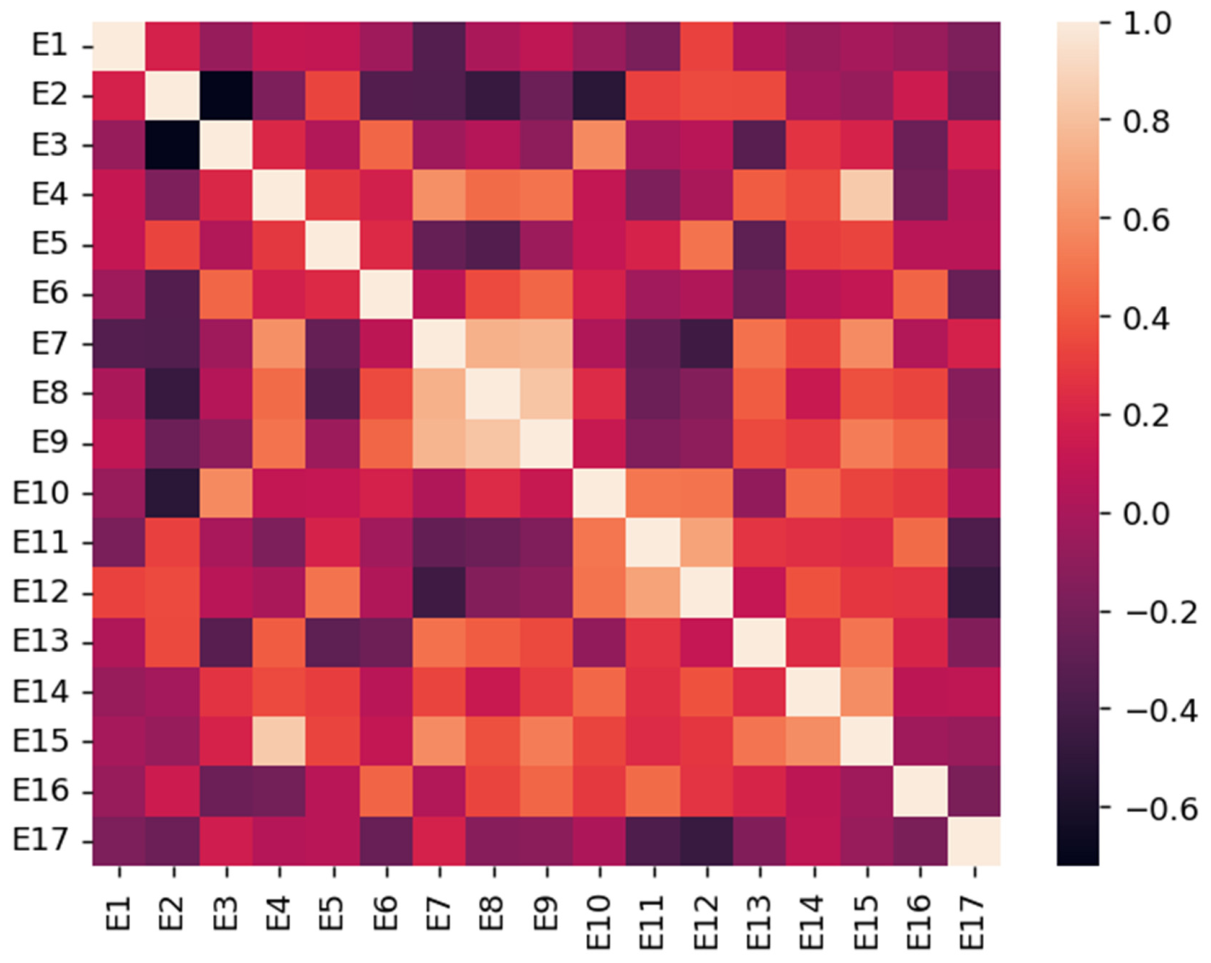
Figure 2.
Ranking genotypes relative to an ideal genotype (located at the center of the concentric circles).
Figure 2.
Ranking genotypes relative to an ideal genotype (located at the center of the concentric circles).
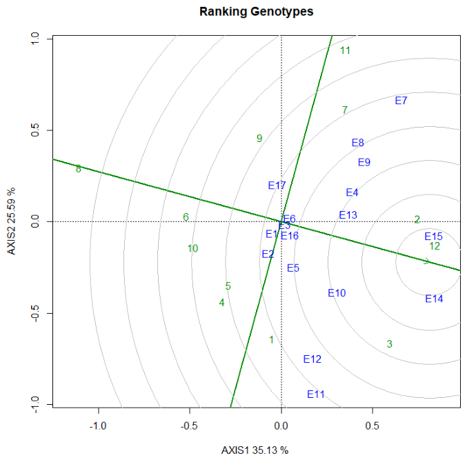
Table 1.
Description of the sunflower testing sites.
| Location | Coordinates | Altitude(masl) | Average Rain fall(mm) | Soil type | Temperature(oc) | |
|---|---|---|---|---|---|---|
| Max | Min | |||||
| Ambo | N8°58′05′′ E37.51′34′′ | 2175 | 1235 | Vertisol | 26 | 12 |
| A/Negele | - | 1496 | 94 | Nitosol | - | - |
| Dera | - | 1650 | 95 | Clay | 19 | 9 |
| Holeta | N09°03′25″ E38°30′26′′ | 2400 | 1044 | Nitosols | 22 | 6 |
| Kulumsa | N08°01′00″ E39°09′32′′ | 2200 | 840 | Clay | 23 | 12 |
| Werer | N9o16′8″ E40o9′41′′ | 740 | 590 | Vertisol | 40 | 19 |
| Worabe | N07°52’21’’ E038°08’42’’ | 2311 | 1312 | Loam | 28 | 14 |
-=not available.
Table 2.
Code, pedigree and sources of sunflower genotypes tested.
| Genotype code | Pedigree | Source |
|---|---|---|
| 1 | Adadi-II-2/1 | HARC |
| 2 | Adadi-II-1/3 | HARC |
| 3 | Adadi-III-1/1 | HARC |
| 4 | Adadi-III-1/4 | HARC |
| 5 | Adadi-III-2/2 | HARC |
| 6 | Adadi-III-2/4 | HARC |
| 7 | Adadi-IV-1/4 | HARC |
| 8 | H-45-1/2 | HARC |
| 9 | NK-Kondi-1/2 | HARC |
| 10 | Adadi-III-2/1 | HARC |
| 11 | Adadi-1 (Check) | HARC |
| 12 | Ayehu (Check) | AARC |
HARC=Holetta Agricultural Research Center, AARC= Adet Agricultural Research Center.
Table 3.
Selected variance-covariance structures for individual environments.
| Env | Best Model | -2LL | AIC | BIC | Residual | SE |
|---|---|---|---|---|---|---|
| E1 | Linear trend across rows | -4.520 | -2.520 | -0.960 | 0.168 | 0.040 |
| E2 | AR order 2 across rows and columns | -43.470 | -33.470 | -25.550 | 0.101 | 0.031 |
| E3 | Random row term | -166.120 | -162.120 | -158.950 | 0.002 | 0.000 |
| E4 | Linear trend across rows | -16.420 | -14.420 | -12.860 | 0.119 | 0.029 |
| E5 | Random row term | -15.380 | -11.380 | -8.210 | 0.131 | 0.037 |
| E6 | Identity across rows and columns | -64.030 | -62.030 | -60.450 | 0.039 | 0.009 |
| E7 | Random row term | -13.360 | -9.360 | -6.190 | 0.125 | 0.035 |
| E8 | Random row and column terms | -73.950 | -67.950 | -63.200 | 0.022 | 0.006 |
| E9 | Linear trend across rows | -9.110 | -7.110 | -5.550 | 0.147 | 0.035 |
| E10 | Identity across rows and columns | -33.090 | -31.090 | -29.500 | 0.092 | 0.022 |
| E11 | Random row term | -22.660 | -18.660 | -15.490 | 0.083 | 0.023 |
| E12 | Random row and column terms | -25.460 | -19.460 | -14.710 | 0.071 | 0.022 |
| E13 | Linear trend across rows and columns | -4.250 | -2.250 | -0.720 | 0.147 | 0.036 |
| E14 | Random row and column terms | -94.320 | -88.320 | -83.570 | 0.009 | 0.003 |
| E15 | Identity across rows and columns | -64.900 | -62.900 | -61.310 | 0.038 | 0.009 |
| E16 | Identity across rows and columns | -35.970 | -33.970 | -32.390 | 0.085 | 0.020 |
| E17 | Identity across rows and columns | -33.190 | -31.190 | -29.600 | 0.092 | 0.022 |
LL=loglikelihood, AIC= Akaike information coefficient, BIC= Schwarz Bayes information coefficient, SE= standard error,Env=environment,E1=Ambo_2023/24,E2=Ambo_2024/25,E3=ArsiNegele_2021/22, 4=ArsiNegele_2024/25, E5=Dera_2024/25,E6=DebreZeit_2021/22,E7=Holeta_2021/22,E8=Holeta_2023/24,E9=Holeta_2024/25,E10=Kulumsa_2021/22, E11=Kulumsa_2022/23, E12=Kulumsa_2023/24,E13=Kulumsa_2024/25, E14=Werer_2023/24, E15=Werer_2024/25, E16=Worabe_2023/24, E17=Worabe_2024/25. The number after underscore indicates the year the trial conducted.
Table 5.
Seed yield (t ha-1) best linear unbiased estimator (BLUE) and stability parameters estimates for test genotypes.
Table 5.
Seed yield (t ha-1) best linear unbiased estimator (BLUE) and stability parameters estimates for test genotypes.
| Genotype code | BLUE | bi | S2di |
|---|---|---|---|
| 1 | 1.265 | 1.063 | 0.033 |
| 2 | 1.394 | 1.210 | 0.012 |
| 3 | 1.358 | 1.262 | 0.014 |
| 4 | 1.159 | 1.048 | 0.012 |
| 5 | 1.161 | 1.120 | 0.007 |
| 6 | 1.122 | 0.952 | 0.016 |
| 7 | 1.237 | 0.899 | 0.045 |
| 8 | 1.057 | 0.695 | 0.034 |
| 9 | 1.177 | 0.850 | 0.023 |
| 10 | 1.135 | 0.897 | 0.020 |
| 11 | 1.229 | 0.884 | 0.066 |
| 12 | 1.347 | 1.122 | 0.029 |
bi = Ebehart & Rusell regression coefficient, S2di=deviation from regression; for designation of genotype’s pedigree name, see Table 2.
Disclaimer/Publisher’s Note: The statements, opinions and data contained in all publications are solely those of the individual author(s) and contributor(s) and not of MDPI and/or the editor(s). MDPI and/or the editor(s) disclaim responsibility for any injury to people or property resulting from any ideas, methods, instructions or products referred to in the content. |
© 2026 by the authors. Licensee MDPI, Basel, Switzerland. This article is an open access article distributed under the terms and conditions of the Creative Commons Attribution (CC BY) license (http://creativecommons.org/licenses/by/4.0/).
Copyright: This open access article is published under a Creative Commons CC BY 4.0 license, which permit the free download, distribution, and reuse, provided that the author and preprint are cited in any reuse.