

Submitted:
28 May 2026
Posted:
01 June 2026
You are already at the latest version
Abstract
Predicting canopy traits non-destructively is important for understanding crop growth and improving phenotyping efficiency. Hyperspectral reflectance provides detailed spectral information, but the role of band selection in regression-based trait prediction at the canopy scale remains unclear. In this study, we evaluated the effects of different band-selection algorithms on the prediction accuracy of aboveground biomass (AGB), leaf area index (LAI), and canopy cover (CC) in soybeans across multiple sites, years, cultivars, and irrigation treatments. We compared a full-band partial least squares regression (PLS) model with three band-selection methods (PLS-Variable Importance in Projection (VIP), Bootstrapped least absolute shrinkage and selection operator (LASSO) (BoLASSO), and an ensemble approach), and model performance was assessed using independent validation datasets. The results showed that the effectiveness of band selection depended on the target trait. Full-band PLS provided the highest accuracy for AGB, whereas BoLASSO achieved comparable accuracy to PLS for LAI and CC using a reduced number of selected bands. The selected wavelengths were located mainly in the visible, red-edge, and near-infrared regions. These results indicate that band-selection strategies should be tailored to the target trait and provide a basis for efficient band design in crop phenotyping.
Keywords:
aboveground biomass
; band selection
; canopy cover
; hyperspectral reflectance
; leaf area index
; soybean
1. Introduction
Soybeans (Glycine max (L.) Merr.) are a globally important crop and a major source of plant-based protein and vegetable oil. They are a staple crop in many countries, including Japan. Advances in breeding and cultivation techniques have led to increased seed yields in many regions [1,2,3]. From a physiological perspective, yield potential under optimal environmental conditions is determined by the radiation interception efficiency (RIE) of the crop canopy, the radiation use efficiency (RUE) that converts this into dry matter, and the harvest index, which indicates the proportion of dry matter allocated to seeds [4]. Recent increases of yield have been primarily associated with increased production of aboveground dry matter [5]. Leaf Area Index (LAI) is closely related to the light interception of the canopy and influences yield formation through RIE [4]. Therefore, monitoring traits such as aboveground biomass (AGB) and LAI over time provides foundational information for the development of high-yielding cultivars.
To elucidate yield formation mechanisms and establish technologies for stable and high yields, it is essential to quantify canopy-level traits. To do so, AGB, LAI, and RIE need to be estimated simultaneously, non-destructively, and rapidly [4,6]. Conventionally, direct measurement methods based on field surveys have been employed. With these methods, plants within a defined area are harvested. AGB is then determined through drying and weighing, and LAI is calculated based on leaf area measurements. RUE is estimated from the relationship between cumulative intercepted radiation and AGB [4,5]. These approaches are highly reliable and have been widely used as standard methods in eco-physiological research and breeding evaluation [5,7,8].
Direct measurement methods, however, are time-consuming and labor-intensive [4,6]. Time-series measurements of AGB require repeated harvesting, drying, and weighing, and the workload increases with the number of samples. Moreover, destructive sampling prevents repeated measurements on the same plants and may affect final yield evaluation. For LAI, both destructive methods [9] and non-destructive approaches such as plant canopy analyzers (e.g., LAI-2200) or aerial photography [10] have been developed, but limitations remain for large-scale, time-series measurements. In soybeans, rapid canopy development further complicates high-throughput evaluation across multiple sites and genotypes [11,12].
In recent years, high-throughput phenotyping technologies have been developed to acquire physiological and agronomic traits non-destructively and at high frequency [11,12,13,14]. Advances in proximal remote sensing, particularly the integration of sensor technologies with data science, have enabled cost-effective phenotyping. Among these, hyperspectral reflectance (HSR) can be used to quantify the vegetation reflectance across a wide spectrum range using hundreds of wavelength bands and to capture the biochemical and structural characteristics of the plant canopy [14,15,16,17,18,19,20].
HSR can be broadly used in two ways: (1) to construct regression models using the full reflectance spectrum as explanatory variables (e.g., partial least squares regression, PLS [21]) and (2) to select spectral regions (features) relevant to the target trait [22]. The former leverages the full spectral signal, whereas the latter includes approaches such as vegetation indices (VIs) based on specific band relationships. These approaches have been applied to estimate various traits, including AGB, LAI, canopy cover (CC), leaf photosynthetic capacity, yield, and nitrogen content [14,17,23,24].
Since HSR data consist of many bands, band selection is not only a means of dimensionality reduction and computational efficiency, but also a key factor influencing predictive performance, generalization, and interpretability [22]. The objectives of band selection can be summarized as: (1) improving the model fit and prediction accuracy [25,26]; (2) enhancing the sensitivity and robustness of vegetation indices for trait prediction [22,27,28]; and (3) improving interpretability by linking spectral features to underlying physiological and molecular processes [29]. Focusing on a subset of bands has been suggested to clarify the relationship between spectral information and traits and improve model applicability across datasets [23,30].
On the other hand, HSR data often exhibit strong correlations among adjacent bands and a limited number of samples relative to the number of variables, which can lead to overfitting and reduced generalization [23,31]. These issues are particularly important in regression tasks [31]. Furthermore, full-band models are sensitive to sensor characteristics and observation conditions, and they may be affected by inter-instrument variations and environmental fluctuations. Practical constraints also exist because hyperspectral sensors are costly and difficult to deploy.
Selecting a limited number of informative bands is considered an effective strategy to improve both the model generalization and practical applicability. However, band-selection results are often dependent on the dataset and analytical procedures, and the selected bands may be unstable [23]. Stepwise regression has been criticized for producing unstable and unreliable band selections [23,29]. Indeed, previous studies have reported a lack of consensus on optimal band sets for chlorophyll estimation [32,33].
Given that no single method has been found to be consistently superior to others [23,33], reliance on a single method is not justified, and frameworks that include inter-method comparisons and stability assessments are required. Ensemble approaches, which combine multiple methods, have been shown to improve prediction accuracy in remote sensing applications [34,35,36,37]. In HSR studies, integrating or stacking multiple machine learning models can enhance prediction accuracy [38]. However, whether such multi-method ensembles enable robust band selection remains unclear [23].
Existing band-selection studies have developed primarily around classification tasks [39], and few frameworks simultaneously evaluate stability, generalization performance, and the interpretability of selected bands in regression tasks involving continuous variables at the canopy scale. Previous reviews have pointed out that redundancy among adjacent bands, limited sample size, and differences in study design (e.g., band range and data composition) hinder the evaluation of generalizability [39].
This study aimed to clarify the effects of different band-selection algorithms on the prediction accuracy of AGB, LAI, and CC for multiple soybean cultivars across different sites, years, cultivars, and irrigation treatments. We specifically tested the hypothesis that models using selected bands can achieve prediction accuracy and generalization performance comparable to those of full-band models under varying observation conditions. In addition, we examined the characteristics of the selected bands to explore their implications for efficient band design and practical applications in remote sensing.
2. Materials and Methods
2.1. Study Sites and Experimental Design
Experiments were conducted over five years (2019, 2020, 2021, 2023, and 2024) at three research centers in Japan: the Tohoku Agricultural Research Center (TARC; 39.74° N, 141.13° E) in Morioka, Iwate; the Institute for Agro-Environmental Sciences (NIAES; 36.02° N, 140.11° E) in Tsukuba, Ibaraki; and the Kyushu-Okinawa Agricultural Research Center (KARC; 33.21° N, 130.49° E) in Chikugo, Fukuoka. Table S1 summarizes the year, site, cultivar, number of replicates, water management conditions, and the number of observations for day of year (DOY), AGB, LAI and CC for each experiment.
Meteorological stations were installed at each site to monitor air temperature, solar radiation, and precipitation. During the growing season (June–October), mean air temperature ranged from 19.5 to 26.6 °C, solar radiation from 14.4 to 17.7 MJ m⁻² d⁻¹, and precipitation from 601 to 1088 mm, with variation among sites and years (Table S2).
At TARC, the soil in the experimental plots was Andosol. In each year, 3 g m⁻² of nitrogen, 12.5 g m⁻² of phosphorus (as P₂O₅), and 5 g m⁻² of potassium (as K₂O) were applied prior to sowing and incorporated into the soil by rotary tillage. The number of cultivars tested was nine in 2019 (Exp. ID 1) and 2020 (Exp. ID 2), six in 2021 (Exp. ID 3), and two in 2023 (Exp. ID 4) and 2024 (Exp. ID 8). Sowing dates were June 5, 2019; June 4, 2020; June 8, 2021; May 30, 2023; and June 18, 2024. All sowing was performed by hand. Seeds were treated with a mixture of insecticide and fungicide (CruiserMaxx, Syngenta Co., Tokyo, Japan) prior to sowing. Immediately after sowing, the prescribed amount of herbicide (Ecotop, Maruwa Biochemical, Tokyo, Japan) was applied, and insecticides and fungicides were sprayed as needed. The planting pattern was 75 cm between rows and 15 cm between plants in all years. The experiment was conducted with three replicates in 2019 and 2020, and two replicates in 2021, 2023, and 2024. The experimental plots consisted of six rows, each 4.8 m long, in 2019 and 2020; nine rows, each 3.0 m long, in 2021; and seven rows, each 3.6 m long, in 2023 and 2024. In 2019, 2020, and 2021, the crops were grown under rain-fed conditions. In 2023, irrigation was applied using irrigation tubes, and three levels of soil moisture—high, medium, and low—were established based on the distance from the tubes. In 2024, irrigation was also performed using irrigation tubes, and two levels of soil moisture—high and low—were established.
At NIAES, the soil in the experimental plots was either Andosol (Exp. IDs 5, 6, and 10) or Typic Endoaquept (Exp. ID 9). In each year, 1.8 g m⁻² of nitrogen, 14 g m⁻² of phosphorus (as P₂O₅), and 6 g m⁻² of potassium (as K₂O) were applied before sowing and incorporated by rotary tillage. The number of test cultivars was two for Exp. ID 5 and four for Exp. ID 6 in 2023, and two for Exp. ID 9 and four for Exp. ID 10 in 2024. Sowing dates were June 13, 2023, and June 11, 2024, and all sowing was done by hand. Seeds were treated with a combined insecticide and fungicide ( ) prior to sowing. Immediately after sowing, the herbicide (Ecotop) was applied at the recommended rate, and insecticides and fungicides were sprayed as needed. The planting pattern was 70 cm between rows and 15 cm between plants in all years. The experiment was conducted with two replicates for Exp. ID 5 and three replicates for Exp. ID 6 in 2023, and two replicates for Exp. ID 9 and three replicates for Exp. ID 10 in 2024. The experimental plots consisted of six rows (7.2 m in length) for Exp. IDs 5 and 9, and six rows (2.5 m) for Exp. IDs 6 and 10. In Exp. ID 5 in 2023, treatments included a rain-fed control, an early-flooding treatment (July 11–13), a late-flooding treatment (July 22–28), and a rain-shielded treatment (July 24–August 6) with rain-fed conditions outside the treatment periods. In Exp. ID 9 (2024), five treatments were established: rain-fed control, early flooding (July 10–16), late flooding (July 26–August 1), combined early and late flooding, and the rain shelter treatment (July 25–August 14).
At KARC, the soil in the experimental plots was Typic Endoaquept. In 2023, no fertilizer was applied. In 2024, 2.4 g m⁻² of nitrogen, 0.9 g m⁻² of phosphorus (as P₂O₅), and 0.2 g m⁻² of potassium (as K₂O) were applied before sowing and incorporated into the soil by rotary tillage. Two cultivars were tested in both 2023 and 2024. Sowing dates were July 15, 2023, and July 17, 2024. Sowing was performed by hand. Seeds were treated with a mixed insecticide and fungicide (CruiserMaxx) prior to sowing. Immediately after sowing, herbicide (Creaturn, Kumiai Chemical Industry Co., Ltd., Tokyo, Japan) was applied at the recommended rate, and insecticides and fungicides were sprayed as needed. The planting pattern was 70 cm between rows and 20 cm between plants. The experiment was conducted with two replicates in both years. The experimental plots consisted of four rows (4.2 m in length) in 2023 and seven rows (1.0 m) in 2024. In 2023, rain-fed (control) and tube-irrigated plots were established. In 2024, a lysimeter equipped with a rain shelter was used, with four treatments: a control with a constant groundwater level of 35 cm, a dry treatment with the water table set at 90 cm (August 19–September 2), an early-stage waterlogged treatment (0 cm; August 2–9), and a late-stage waterlogged treatment (0 cm; August 19–26).
2.2. Ground Truth Data for AGB, LAI, and CC
At TARC, destructive surveys to measure AGB and LAI were conducted four times in 2019 (Exp. ID 1) and 2020 (Exp. ID 2), twice in 2021 (Exp. ID 3), three times in 2023 (Exp. ID 4), and twice in 2024 (Exp. ID 8) (Table S1). In Exp. IDs 1–3, 0.68 m² was harvested from three rows in each plot. In Exp. IDs 4 and 8, 0.45 m² was harvested from one row in each plot.
At NIAES, destructive surveys were conducted once for Exp. ID 5 and six times for Exp. ID 6 in 2023, and once for Exp. ID 9 and nine times for Exp. ID 10 in 2024. In Exp. IDs 5 and 9, 0.42 m² was harvested from one row in each plot, whereas in Exp. IDs 6 and 10, 0.84 m² was harvested from four rows in each plot.
At KARC, destructive surveys were conducted once in each of 2023 (Exp. ID 7) and 2024 (Exp. ID 11). In Exp. ID 7, 0.56 m² was harvested from one row in each plot, and in Exp. ID 11, 0.84 m² was harvested from two rows in each plot.
As described in Section 2.3, because the sensor footprint was approximately 0.35 m², all sampling areas sufficiently covered the measurement area.
Leaves were separated from the collected plant material, and leaf area was measured. At TARC, an automatic leaf area meter (AAM-8, Hayashidenko Co., Ltd., Tokyo, Japan) was used, whereas at NIAES and KARC, a leaf area meter (LI-3100C, LI-COR, Lincoln, NE, USA) was used. LAI was calculated by dividing leaf area by sampling area. After drying the plant samples at 80 °C for three days, total dry weight was measured and converted to AGB based on the sampling area.
Fractional canopy cover (CC) was estimated using digital image analysis at TARC and NIAES. Images were captured using a camera (GACS1; Kimura Ouyou-Kougei Co., Ltd., Osaka, Japan) mounted at a height of 1.5 m above ground level and pointing directly downward (nadir). CC was calculated according to the method of Kumagai and Takahashi [40]. Imaging was conducted at time points corresponding to the destructive surveys. Data for 2021 at TARC and some observations at other sites were missing (the “0” values in Table S1).
2.3. Measurement of Canopy HSR
In this study, to obtain canopy scale HSR at high frequency in experimental plots where multiple cultivars were grown, we developed a portable measurement system. Drawing on the method described by Kimm et al. [41], we adopted a single-fiber configuration to reduce weight and simplify the system. The configuration of the measurement system and the observation geometry are shown in Figure S1.
The Flame-S spectrometer (Ocean Insight Inc., Orlando, FL, USA) was used for the measurements. This instrument measures wavelengths in the 501–801 nm range and has a spectral resolution of 0.92 nm (FWHM). A fiber with a core diameter of 600 μm (Ocean Insight) was used. Incident light was measured using a standard reflector (Spectralon, Labsphere Inc., North Sutton, NH, USA), and upward radiation from the canopy was measured with at a field of view of 25°. Reflectance was calculated as the ratio of the two measurements.
The fiber tip was fixed approximately 1.5 m above the ground, and a level was used to confirm a zenith angle of 0° (nadir) during measurements. Three to five measurements were taken per plot, and the average value was used as the representative value. The measurement time per plot was less than one minute. Standard reflector measurements were performed before each plot measurement. Dark current was acquired by blocking the light path using an INLINE-TTL-S Electronic Shutter (Ocean Insight), and corrections were made with particular attention to fluctuations in solar irradiance and temperature. When solar irradiance changed, the integration time was adjusted using a standard reflector to avoid saturation of the DN values. Measurements were conducted between 10:00 and 15:00 on clear days, before and after the destructive surveys for AGB and LAI. The acquired data were recorded using OceanView software (Ocean Insight) and smoothed using a Savitzky–Golay filter (third-order polynomial, 9-band moving window) [42]. Subsequently, the spectral bands were rounded to the nearest integer at 1-nm intervals using custom R scripts, and the processed data were used for analysis.
2.4. Model Development and Validation
Machine learning regression models were applied to predict AGB, LAI, and CC using visible-near-infrared (VNIR) spectral reflectance data (301 bands, 501–801 nm) at the canopy scale. Prior to model development, outliers were removed as part of data quality control. Following Montes et al. [43], a two-step outlier detection procedure was applied based on the target variables and PLS residuals.
First, for each target variable (AGB, LAI, and CC), outliers were identified based on the interquartile range (IQR), and values below Q1 − 1.5 × IQR or above Q3 + 1.5 × IQR were removed. Next, a PLS model was constructed using the remaining data, and residuals between the observed and predicted values were calculated. PLS is effective for high-dimensional spectral data with strong multicollinearity because it extracts latent variables that maximize covariance between explanatory variables and target variables [21]. The optimal number of latent variables was determined using 5-fold cross-validation after standardization.
Outlier detection based on the IQR was then applied to the residuals, and identified samples were removed. These procedures reduced the influence of measurement errors and improved the model’s stability and generalization performance. A total of 472, 462, and 390 samples were collected for AGB, LAI, and CC, respectively (Table S1). After outlier removal, 464, 447, and 380 samples remained, respectively. The proportions of removed samples were 1.7%, 3.2%, and 2.6% for AGB, LAI, and CC, respectively.
The dataset was divided into training and validation sets in a 2:1 ratio using the Kennard–Stone algorithm [44], which selects representative samples to evenly cover the data space based on distances in multivariate space.
Taking practical applications into account, the number of selected bands used as explanatory variables in the final model was limited to 10. This was intended to enable implementation using 10-band multispectral cameras (e.g., the MicaSense dual camera system) mounted on commercially available UAVs. In this study, we compared PLS using all bands; variable importance in projection (VIP), which extracts bands with high contribution from the PLS model (PLS-VIP); bootstrapped least absolute shrinkage and selection operator (LASSO) (BoLASSO), which mitigates the selection instability of LASSO using bootstrapping; and an ensemble method that integrates band importance based on multiple regression models.
In PLS-VIP, we first standardized the explanatory and response variables and determined the optimal number of latent variables via cross-validation to construct a PLS model. Next, we calculated VIP scores for each band to evaluate their contribution to the model. The VIP score is an indicator calculated by integrating the score, weight, and relationship with the response variable for each latent variable; higher values indicate greater contributions to the prediction [21]. Subsequently, the top 10 bands were selected based on the VIP scores, and unnecessary variables were removed using stepwise backward selection based on the Akaike information criterion (AIC) to determine the final combination of explanatory variables.
The workflows for BoLASSO and the ensemble method are shown in Figure 1. BoLASSO was applied with some modifications to the method proposed by Bach [45]. First, the explanatory variables and response variable in the training data were standardized, and the LASSO regularization parameter was determined using 5-fold cross-validation. Subsequently, 1000 bootstrap samples were generated, and LASSO regression was applied to each sample. For each band, the number of times the regression coefficient was non-zero was counted as the selection frequency, and the top 10 bands with the highest selection frequencies were extracted. Using these 10 bands as candidate variables, unnecessary variables were removed using an AIC-based sequential variable reduction method to construct the final multiple regression model.
For the ensemble method, we referred to the approach by Feilhauer et al. [22]. Band importance was calculated using four methods: PLS, Ridge regression, LASSO, and linear support vector regression (LSVR). For each method, the absolute value of the standardized regression coefficient was used as the importance score. The importance scores from each method were weighted by the coefficient of determination (R²) from cross-validation and summed across methods to calculate the ensemble importance (IE). The top 10 bands were selected based on IE, and similar to BoLASSO, a final multiple regression model was constructed using an AIC-based sequential variable reduction method.
The prediction accuracy of the models was evaluated using the coefficient of determination (R²) and root mean square error (RMSE) for both the training and validation data. Furthermore, the normalized RMSE (nRMSE, %) was calculated by dividing the RMSE by the mean of the observed values and multiplying by 100.
The hyperparameters for each regression method were optimized using cross-validation. Specifically, for PLS, the number of latent variables was determined; for Ridge and LASSO, the regularization parameters were determined; and for LSVR, the regularization coefficient and ε were determined.
Data analysis and visualization were performed in Python using Jupyter Notebook and the Scikit-learn, Pandas, NumPy, Statsmodels, SciPy, and Matplotlib libraries.
3. Results
3.1. Data Characteristics
Figure 2 shows the average and range of spectral reflectance in the visible to near-infrared region (501–801 nm). Reflectance remained low in the visible region (500–700 nm), with strong absorption observed particularly in the red region. In contrast, reflectance increased sharply beyond approximately 700 nm, confirming the characteristic red edge feature. The mean reflectance varied systematically with wavelength, and the standard deviation (SD) tended to increase in the near-infrared region. Furthermore, the ranges of maximum and minimum values also expanded in the near-infrared region, indicating that data variability was wavelength-dependent.
Table 1 shows the descriptive statistics for AGB, LAI, and CC. AGB ranged widely from 8 to 1188 g m⁻², with a mean of 374 g m⁻² and a high coefficient of variation (CV) of 74%. LAI ranged from 0.26 to 8.65 m² m⁻², with a mean of 3.80 and a CV of 53%. CC ranged from 5 to 100%, with a mean of 82% and a relatively low CV of 28%. These results indicate that the dataset covered a wide variation in growth stages and canopy structures.
3.2. Effect of Different Band-Selection Algorithms on AGB Prediction Accuracy
We compared the prediction accuracy of AGB between PLS models using all bands and three types of band-selection models (PLS-VIP, BoLASSO, and the ensemble method) (Table 2, Figures S2 and S3). In the training data, all methods exhibited relatively high coefficients of determination; however, PLS-VIP showed large variability in predicted values, with both underestimation and overestimation (Figure S2). In contrast, BoLASSO and the ensemble method showed close relationships between observed and predicted values along the 1:1 line, confirming stable reproducibility. In the validation data, the full-band PLS model exhibited the highest coefficient of determination (R² = 0.786) and the lowest normalized RMSE (nRMSE = 28.8%) (Table 2, Figure S3). Although BoLASSO (R² = 0.697, nRMSE = 34.3%) and the ensemble method (R² = 0.604, nRMSE = 39.3%) showed slightly lower accuracy than the full-band PLS model, they maintained relatively high prediction accuracy. In contrast, PLS-VIP showed substantially lower accuracy (R² = 0.369 and nRMSE = 49.5%).
As a result of band selection, BoLASSO selected wavelengths of 520, 525, 607, 692, and 695 nm in the visible region and 716, 739, and 793 nm in the near-infrared region (Table 2). The ensemble method also selected wavelengths in the visible region (520, 594, 606–607, and 683 nm) and the near-infrared region (716 and 792–793 nm), showing a common tendency for important wavelengths to be concentrated in the green to red and red-edge to near-infrared regions. In contrast, PLS-VIP selected wavelengths of 677–683 nm and 762–797 nm; however, fewer bands were selected, and the prediction accuracy was lower than that of the other methods. The number of explanatory variables was 301 bands in the full-band PLS model, whereas it was reduced to 6–8 selected bands in the band-selection models (Table 2). These results indicate that BoLASSO and the ensemble method can maintain prediction accuracy with a reduced number of selected bands, whereas the PLS-VIP shows a marked decline in accuracy associated with band reduction.
Overall, differences in band-selection algorithms affected AGB prediction accuracy and the distribution of selected wavelengths, suggesting that efficient AGB prediction using a small number of selected bands is feasible when appropriate methods are used.
3.3. Effect of Different Band-Selection Algorithms on LAI Prediction Accuracy
We compared the accuracy of LAI prediction between the PLS model using all bands and the three band-selection models (Table 3, Figures S4 and S5). In the training data, all methods exhibited relatively high coefficients of determination, and the observed and predicted values were generally distributed along a 1:1 line (Figure S4). However, PLS-VIP showed slightly greater variability than the other methods. In the validation data, BoLASSO exhibited the highest coefficient of determination (R² = 0.828) and the lowest normalized RMSE (nRMSE = 21.4%), demonstrating accuracy comparable to that of the full-band PLS model (R² = 0.823, nRMSE = 21.8%) (Table 3, Figure S5). The ensemble method (R² = 0.795, nRMSE = 23.4%) exhibited slightly lower accuracy than these two methods but maintained relatively high prediction accuracy. In contrast, PLS-VIP showed lower accuracy than the other methods (R² = 0.736 and nRMSE = 26.5%).
As a result of band selection, BoLASSO selected wavelengths of 501, 504, 704, 732, 793, and 796 nm, distributed across the visible region (blue to green) and the red-edge to near-infrared regions (Table 3). The ensemble method also selected wavelengths of 501, 704, 727, 732, and 785, 786 nm, showing a tendency for important wavelengths to be concentrated particularly in the red-edge to near-infrared regions. In contrast, PLS-VIP selected wavelengths of 502 nm and 762–798 nm; however, the distribution was broader and less consistent than those of the other methods. The number of explanatory variables was reduced to 6–7 selected bands in the band-selection models (Table 3). These results indicate that BoLASSO and the ensemble method can maintain high prediction accuracy with a reduced number of selected bands, whereas the PLS-VIP showed a decline in accuracy with band reduction.
In summary, differences in band-selection algorithms affected LAI prediction accuracy and the distribution of selected wavelengths, indicating that efficient LAI prediction using a small number of selected bands is possible when appropriate methods are used.
3.4. Effect of Differences in Band-Selection Algorithms on the Accuracy of CC Prediction
We compared the accuracy of canopy cover (CC) estimation between the PLS model using all bands and the three types of band-selection models (Table 4, Figures S6 and S7). In the training data, all methods exhibited high coefficients of determination, and the observed and predicted values were generally distributed along a 1:1 line (Figure S6). However, PLS-VIP showed greater variability than the other methods, and a decrease in prediction accuracy was observed, particularly in the high CC range. In the validation data, BoLASSO exhibited the highest coefficient of determination (R² = 0.894) and demonstrated accuracy comparable to that of the full-band PLS model (R² = 0.893) (Table 4, Figure S7). Both methods showed the same normalized RMSE (nRMSE = 7.7%) and high prediction accuracy. The ensemble method (R² = 0.843, nRMSE = 9.35%) exhibited slightly lower accuracy than these two methods but maintained relatively high accuracy. In contrast, PLS-VIP showed lower accuracy than the other methods (R² = 0.630 and nRMSE = 14.4%).
As a result of band selection, BoLASSO selected wavelengths in the visible region at 549, 599, and 610 nm, the red region at 683 and 694 nm, and the red-edge to near-infrared regions at 720, 724, 762, and 793 nm (Table 4). In the ensemble method, wavelengths in the visible region (535, 599, and 683 nm) and the red-edge to near-infrared region (720, 762, and 797 nm) were selected, indicating a tendency for important wavelengths to be distributed across a wide range from the visible to near-infrared regions. In contrast, PLS-VIP selected wavelengths concentrated in the near-infrared region (763–798 nm), but its accuracy was lower than that of the other methods. The number of explanatory variables was reduced to 5–9 selected bands in the band-selection models (Table 4). These results indicate that while BoLASSO and the ensemble method can maintain high accuracy even with a reduced number of selected bands, PLS-VIP exhibited a decrease in accuracy with the reduction in bands.
Overall, these findings suggest that differences in band-selection algorithms affect the accuracy of CC prediction and the distribution of selected wavelengths, and that efficient CC prediction using a small number of selected bands is feasible when appropriate methods are employed.
4. Discussion
4.1. Trait-Dependent Effects of Band Selection on Model Performance
This study compared the effects of different band-selection algorithms on the prediction accuracy of AGB, LAI, and CC in soybean canopies. We specifically examined whether models using selected bands could achieve prediction accuracy comparable to that of full-band PLS models under varying conditions of sites, years, cultivars, and irrigation levels. HSR has been widely used to estimate crop canopy traits such as biomass, LAI-related variables, and nitrogen status, but prediction performance often varies depending on the target trait and spectral modeling approach [15,16,17,18,19,20]. The results showed that the effectiveness of band selection depends on the target trait. For AGB, the full-band PLS model achieved the highest accuracy, whereas band selection resulted in some loss of accuracy (Table 2). In contrast, for LAI and CC, BoLASSO achieved accuracy comparable to that of the full-band PLS model, maintaining high prediction accuracy with a reduced number of selected bands (Table 3 and Table 4). These results are consistent with previous studies showing that useful spectral information and model performance can vary among soybean crop variables and other canopy traits [17,19,20].
This trait-dependent response likely reflects the complexity of the canopy information represented by each trait. AGB is an integrated trait representing dry matter accumulation, including leaves, stems, and pods, and it is influenced by multiple factors such as organ allocation and growth stage [4,5,6]. In contrast, LAI and CC are more directly related to canopy leaf area and cover, which are more strongly reflected in canopy spectral signals [9,10,40]. Therefore, band selection should not be regarded simply as a method for reducing dimensionality but as a trait-specific modeling step that needs to balance prediction accuracy, model simplicity, and biological interpretability [23,25,39].
4.2. Physiological Interpretation of Selected Wavelengths
To further interpret the trait-dependent differences described above, we examined the physiological meaning of the selected wavelengths. In this study, the selected wavelengths were primarily concentrated in the visible, red-edge, and near-infrared regions. For AGB, wavelengths around 520 nm, 600–700 nm, and 716–793 nm were selected using BoLASSO and the ensemble method (Table 2). For LAI, wavelengths of 501–504 nm, 704 nm, 727–732 nm, and 785–796 nm were selected (Table 3), while for CC, wavelengths of 549–610 nm, 683–694 nm, 720–724 nm, and 762–797 nm were selected (Table 4). These wavelength ranges are associated with absorption by leaf pigments, shifts in the red-edge position, and changes in near-infrared reflectance related to leaf area and canopy structure. Wavelengths in the visible region are primarily influenced by the absorption of pigments such as chlorophyll. The red region, in particular, is strongly related to chlorophyll absorption and reflects changes in stand biomass and green leaf mass. The red-edge region around 700 nm represents the transition from strong absorption in the red region to high reflectance in the near-infrared region and is highly sensitive to LAI, chlorophyll content, and canopy condition [22,27,28]. Furthermore, reflectance in the near-infrared region is influenced by leaf internal structure and multiple scattering within the canopy, making it effective for estimating structural traits such as LAI and CC [14,15,16,17,18,19,20]. The high accuracy observed for LAI and CC with a small number of bands suggests that these traits are strongly governed by structural information in the red-edge to near-infrared region.
In contrast, for AGB, accuracy decreased when the number of selected bands was reduced. This likely reflects the fact that AGB represents total dry matter accumulation, including stems and pods, and thus includes components that are not fully captured by canopy surface reflectance in the visible and near-infrared regions alone. Therefore, although selected wavelengths can be physiologically interpreted, the broader spectral information retained in the full-band model likely contributed to the improved accuracy.
4.3. Differences Among Band-selection Algorithms
Differences in band-selection algorithms also had a marked impact on prediction accuracy and the stability of the selected bands. BoLASSO achieved accuracy comparable to that of the full-band PLS model for LAI and CC and maintained a relatively high level of accuracy for AGB (Table 2, Table 3 and Table 4). This likely reflects the fact that bootstrap-based variable selection extracts stable bands contributing to trait prediction while reducing redundancy among adjacent bands. Bootstrapping is widely used to improve the stability of variable selection [45] and has been shown to suppress overfitting and selection bias in high-dimensional data. In hyperspectral data, strong correlations among adjacent bands and a large number of explanatory variables relative to the number of samples often lead to overfitting and instability in band selection [23,31]. The present results indicate that appropriate band selection can maintain prediction accuracy and interpretability while reducing redundant information.
Although the ensemble method showed slightly lower accuracy than BoLASSO, it outperformed PLS-VIP, likely reflecting the fact that integrating multiple methods mitigates the instability associated with relying on a single approach. Ensemble strategies have been widely used in remote sensing to improve prediction accuracy and robustness [34,35,36,37,38]. The results of this study suggest that ensemble-based band selection is effective for constructing practical models using a limited number of selected bands.
In contrast, PLS-VIP showed lower accuracy than the other methods for all three traits. PLS-VIP evaluates band importance based on contributions to latent variables in a PLS model; however, this evaluation depends on the structure of the latent variables [21]. In hyperspectral data, where adjacent bands are highly correlated, the tendency of importance to be distributed across neighboring bands makes it difficult to stably select specific bands. Such multicollinearity has been reported to cause instability in variable selection and reduce estimation accuracy [46].
4.4. Implications for Remote Sensing Applications and Future Work
The results of this study indicate that, in predicting soybean canopy traits using HSR, band selection is not merely a matter of reducing dimensionality but a critical process that influences prediction accuracy, generalization performance, and interpretability. This conclusion is consistent with previous studies showing that hyperspectral reflectance can provide useful information for estimating crop canopy traits, including biomass, LAI-related variables, nitrogen status, and biochemical traits [15,16,17,18,19,20,22,24]. In particular, for LAI and CC, accuracy comparable to that of the full-band PLS model was maintained even with a small number (6–9) of selected bands. This provides useful insights for the design of simple multispectral sensors independent of hyperspectral systems, as well as for implementation in UAV- and ground-based phenotyping platforms [11,12,13,14].
Since the full-band PLS model showed the highest accuracy for AGB prediction, reducing the number of selected bands is not always effective for all traits. For traits influenced by multiple organs or growth stages, such as AGB, there may be a trade-off between model simplification and estimation accuracy. Previous studies have also shown that the performance of spectral models depends on the target trait and growth stage, and that full-spectrum or multivariate approaches can be advantageous when canopy traits are controlled by multiple structural and physiological factors [17,18,19,20]. Therefore, in practical applications, the choice between full-band and reduced-band models should depend on the target trait.
Our study has several limitations. First, the band range was limited to 501–801 nm and did not include regions such as the shortwave infrared region that are related to nitrogen content, moisture content, or dry matter composition [29]. Considering that full-band PLS was advantageous for AGB prediction, using a broader spectral range may further improve accuracy. Second, this study was based on ground-based, canopy-scale reflectance data; thus, direct application to UAV or satellite observations requires consideration of factors such as observation angle, spatial resolution, atmospheric correction, and background soil effects [11,12,13]. Third, although multiple sites, years, cultivars and irrigation treatments were included, representing a wide range of climatic conditions in Japan, further validation is needed for different climate zones, cropping systems, and cultivars. In addition, although the Kennard–Stone algorithm provided representative training and validation datasets, external validation across independent years, sites, or cultivars remains necessary to fully evaluate model transferability.
Overall, this study demonstrated that differences in band-selection algorithms affect both prediction accuracy and the interpretation of selected wavelengths for soybean canopy traits. In particular, the fact that BoLASSO maintained accuracy comparable to full-band PLS for LAI and CC using fewer bands highlighted its potential for efficient band design and practical applications. In contrast, for AGB, the fact that full-spectrum information remained advantageous indicated the need for trait-specific band-selection strategies.
Furthermore, the results indicate that both AGB and CC can be predicted simultaneously by HSR. Because CC is directly related to canopy light interception and AGB represents dry matter accumulation, their combined estimation provides a practical framework for non-destructive, high-throughput estimation of RUE. While conventional RUE estimation requires repeated destructive sampling and radiation measurements [4,5,6,7,40], this approach enables rapid, non-destructive evaluation of canopy productivity under field conditions.
5. Conclusions
This study evaluated the impact of different band-selection algorithms on the accuracy of predicting soybean canopy traits. The results showed that the effectiveness of band selection depends on the target trait. While the full-band model provided the highest accuracy for AGB, comparable accuracy was achieved for LAI and CC with a limited number of selected bands.
The concentration of selected wavelengths in the visible, red-edge, and near-infrared regions reflected the physiological and structural characteristics of the canopy. These findings highlight the importance of trait-specific band-selection strategies and demonstrate the potential for efficient band design in remote sensing applications.
Supplementary Materials
The following supporting information can be downloaded at the website of this paper posted on Preprints.org.
Author Contributions
Conceptualization, E.K.; methodology, E.K.; formal analysis, E.K.; investigation, E.K., T.Y., Y.M., K.K., E.F., and R.N; resources, E.K., T.Y., Y.M., K.K., E.F., and R.N.; data curation, E.K.; writing—original draft preparation, E.K.; writing—review and editing, T.Y., Y.M., K.K., E.F., and R.N.; visualization, E.K.; supervision, E.K.; project administration, E.K.; funding acquisition, E.K. All authors have read and agreed to the published version of the manuscript.
Funding
This research was supported by the Cross-ministerial Strategic Innovation Promotion Program (SIP), ”Building a sustainable food chain that provides abundant and nutritious food (tentative)” (funding agency: Bio-oriented Technology Research Advancement Institution) and by the Japan Society for the Promotion of Science (JSPS) KAKENHI (Grant Numbers JP18H02190 and JP23K26892).
Data Availability Statement
The data that supports the findings of this study are available from the corresponding author upon reasonable request.
Acknowledgments
We thank Toshihiro Hasegawa, Eri Ogiso-Tanaka, Kaori Hirata, Tetsuya Yamada, Kazumi Suenaga, Ayumi Hatakeyama, Toyoshi Omizu, Hirokazu Tomiyama, Takahiro Mikuni, Akihito Okubo, Kanae Saito, Yuki Muta, Rina Suzuki, Hiroyuki Kato, Yoshihiro Nakao, Tomoe Abe, Kohei Nishiya, Hiroko Yamaura, Miyuki Nakajima, Mari Namikawa, Kafumi Segawa, Yuko Suzuki, Erika Sasaki, Koya Yoshida, Hisashi Tamura, Eisaku Kumagai, Fumihiko Saito, Hisaya Tanaka, Hiroshi Kawamukai, Yuto Omori, Yasuaki Kamata, Koki Yamato, Haruko Shimoda, Yasutaka Kawaguchi, Masao Minamoto, Isao Aoki, Kazumi Tominaga, and Kanako Tanaka (NARO) for their technical assistance. We also thank the members of the SIP project for their valuable comments and constructive suggestions on the methodological aspects of this study. During the preparation of this manuscript, the authors used ChatGPT through Microsoft Copilot to support language editing, grammar checking, and readability improvement. The authors reviewed and edited all AI-assisted outputs and take full responsibility for the content of the manuscript.
Conflicts of Interest
The authors declare no conflicts of interest.
References
- Jin, J.; Liu, X.; Wang, G.; Mi, L.; Shen, Z.; Chen, X.; Herbert, S.J. Agronomic and physiological contributions to the yield improvement of soybean cultivars released from 1950 to 2006 in northeast China. Field Crop. Res. 2010, 115, 116–123. [Google Scholar] [CrossRef]
- Rincker, K.; Nelson, R.; Specht, J.; Sleper, D.; Cary, T.; Cianzio, S.R.; Casteel, S.; Conley, S.; Chen, P.; Davis, V.; et al. Genetic improvement of U.S. soybean in maturity groups ii, iii, and iv. Crop Sci. 2014, 54, 1419–1432. [Google Scholar] [CrossRef]
- Todeschini, M.H.; Milioli, A.S.; Rosa, A.C.; Dallacorte, L.V.; Panho, M.C.; Marchese, J.A.; Benin, G. Soybean genetic progress in south brazil: Physiological, phenological and agronomic traits. Euphytica 2019, 215. [Google Scholar] [CrossRef]
- Monteith, J.L. Climate and efficiency of crop production in britain. Philos. Trans. R. Soc. Lond. B Biol. Sci. 1977, 281, 277–294. [Google Scholar] [CrossRef]
- Koester, R.P.; Skoneczka, J.A.; Cary, T.R.; Diers, B.W.; Ainsworth, E.A. Historical gains in soybean (Glycine max Merr.) seed yield are driven by linear increases in light interception, energy conversion, and partitioning efficiencies. J. Exp. Bot. 2014, 65, 3311–3321. [Google Scholar] [CrossRef]
- Sinclair, T.R.; Muchow, R.C. Occam's Razor, Radiation-use efficiency, and vapor pressure deficit. Field Crop. Res. 1999, 62, 239–243. [Google Scholar] [CrossRef]
- Kumagai, E.; Yabiku, T.; Hasegawa, T. A strong negative trade-off between seed number and 100-seed weight stalls genetic yield gains in northern Japanese soybean cultivars in comparison with Midwestern US cultivars. Field Crop. Res. 2022, 283. [Google Scholar] [CrossRef]
- Murcia, M.A.L.; Moreira, F.F.; Hearst, A.; Cherkauer, K.; Rainey, K.M. Physiological breeding for yield improvement in soybean: solar radiation interception-conversion, and harvest index. Theor. Appl. Genet. 2022. [Google Scholar] [CrossRef]
- Watson, D.J. Comparative physiological studies on the growth of field crops: I. Variation in net assimilation rate and leaf area between species and varieties, and within and between years. Ann. Bot. 1947, 11, 41–76. [Google Scholar] [CrossRef]
- Welles, J.M.; Norman, J.M. Instrument for indirect measurement of canopy architecture. Agron. J. 1991, 83, 818–825. [Google Scholar] [CrossRef]
- Luis Araus, J.; Cairns, J.E. Field high-throughput phenotyping: The new crop breeding frontier. Trends Plant Sci. 2014, 19, 52–61. [Google Scholar] [CrossRef]
- Borra-Serrano, I.; De Swaef, T.; Quataert, P.; Aper, J.; Saleem, A.; Saeys, W.; Somers, B.; Roldán-Ruiz, I.; Lootens, P. Closing the phenotyping gap: High resolution UAV time series for soybean growth analysis provides objective data from field trials. Remote Sens. 2020, 12. [Google Scholar] [CrossRef]
- White, J.W.; Andrade-Sanchez, P.; Gore, M.A.; Bronson, K.F.; Coffelt, T.A.; Conley, M.M.; Feldmann, K.A.; French, A.N.; Heun, J.T.; Hunsaker, D.J.; et al. Field-based phenomics for plant genetics research. Field Crop. Res. 2012, 133, 101–112. [Google Scholar] [CrossRef]
- Fu, P.; Montes, C.M.; Siebers, M.H.; Gomez-Casanovas, N.; McGrath, J.M.; Ainsworth, E.A.; Bernacchi, C.J. Advances in field-based high-throughput photosynthetic phenotyping. J. Exp. Bot. 2022, 73, 3157–3172. [Google Scholar] [CrossRef]
- Flynn, K.C.; Baath, G.; Lee, T.O.; Gowda, P.; Northup, B. Hyperspectral reflectance and machine learning to monitor legume biomass and nitrogen accumulation. Comput. Electron. Agric. 2023, 211. [Google Scholar] [CrossRef]
- Vollmann, J.; Rischbeck, P.; Pachner, M.; Đorđević, V.; Manschadi, A.M. High-throughput screening of soybean di-nitrogen fixation and seed nitrogen content using spectral sensing. Comput. Electron. Agric. 2022, 199. [Google Scholar] [CrossRef]
- Chiozza, M.V.; Parmley, K.A.; Higgins, R.H.; Singh, A.K.; Miguez, F.E. Comparative prediction accuracy of hyperspectral bands for different soybean crop variables: From leaf area to seed composition. Field Crop. Res. 2021, 271. [Google Scholar] [CrossRef]
- Kawamura, K.; Ikeura, H.; Phongchanmaixay, S.; Khanthavong, P. Canopy hyperspectral sensing of paddy fields at the booting stage and pls regression can assess grain yield. Remote Sens. 2018, 10. [Google Scholar] [CrossRef]
- Gnyp, M.L.; Miao, Y.; Yuan, F.; Ustin, S.L.; Yu, K.; Yao, Y.; Huang, S.; Bareth, G. Hyperspectral canopy sensing of paddy rice aboveground biomass at different growth stages. Field Crop. Res. 2014, 155, 42–55. [Google Scholar] [CrossRef]
- Hansen, P.M.; Schjoerring, J.K. Reflectance measurement of canopy biomass and nitrogen status in wheat crops using normalized difference vegetation indices and partial least squares regression. Remote Sens. Environ. 2003, 86, 542–553. [Google Scholar] [CrossRef]
- Wold, S.; Sjöström, M.; Eriksson, L. PLS-regression: a basic tool of chemometrics. Chemom. Intell. Lab. Syst. 2001, 58, 109–130. [Google Scholar] [CrossRef]
- Feilhauer, H.; Asner, G.P.; Martin, R.E. Multi-method ensemble selection of spectral wavelengths related to leaf biochemistry. Remote Sens. Environ. 2015, 164, 57–65. [Google Scholar] [CrossRef]
- Inoue, Y.; Guerif, M.; Baret, F.; Skidmore, A.; Gitelson, A.; Schlerf, M.; Darvishzadeh, R.; Olioso, A. Simple and robust methods for remote sensing of canopy chlorophyll content: A comparative analysis of hyperspectral data for different types of vegetation. Plant Cell Environ. 2016, 39, 2609–2623. [Google Scholar] [CrossRef]
- Kumagai, E.; Burroughs, C.H.; Pederson, T.L.; Montes, C.M.; Peng, B.; Kimm, H.; Guan, K.; Ainsworth, E.A.; Bernacchi, C.J. Predicting biochemical acclimation of leaf photosynthesis in soybean under in-field canopy warming using hyperspectral reflectance. Plant Cell Environ. 2022, 45, 80–94. [Google Scholar] [CrossRef]
- Andersen, C.M.; Bro, R. Variable selection in regression—a tutorial. J. Chemom. 2010, 24, 728–737. [Google Scholar] [CrossRef]
- Genuer, R.; Poggi, J.-M.; Tuleau-Malot, C. Variable selection using random forests. Pattern Recognit. Lett. 2010, 31, 2225–2236. [Google Scholar] [CrossRef]
- Blackburn, G.A. Spectral indices for estimating photosynthetic pigment concentrations: A test using senescent tree leaves. Int. J. Remote Sens. 1998, 19, 657–675. [Google Scholar] [CrossRef]
- Sims, D.A.; Gamon, J.A. Relationships between leaf pigment content and spectral reflectance across a wide range of species, leaf structures and developmental stages. Remote Sens. Environ. 2002, 81, 337–354. [Google Scholar] [CrossRef]
- Curran, P.J. Remote sensing of foliar chemistry. Remote Sens. Environ. 1989, 30, 271–278. [Google Scholar] [CrossRef]
- Kokaly, R.F.; Clark, R.N. Spectroscopic determination of leaf biochemistry using band-depth analysis of absorption features and stepwise multiple linear regression. Remote Sens. Environ. 1999, 67, 267–287. [Google Scholar] [CrossRef]
- Fu, Y.; Yang, G.; Pu, R.; Li, Z.; Li, H.; Xu, X.; Song, X.; Yang, X.; Zhao, C. An overview of crop nitrogen status assessment using hyperspectral remote sensing: Current status and perspectives. Eur. J. Agron. 2021, 124. [Google Scholar] [CrossRef]
- Blackburn, G.A. Hyperspectral remote sensing of plant pigments. J. Exp. Bot. 2006, 58, 855–867. [Google Scholar] [CrossRef] [PubMed]
- Ustin, S.L.; Gitelson, A.A.; Jacquemoud, S.; Schaepman, M.; Asner, G.P.; Gamon, J.A.; Zarco-Tejada, P. Retrieval of foliar information about plant pigment systems from high resolution spectroscopy. Remote Sens. Environ. 2009, 113, S67–S77. [Google Scholar] [CrossRef]
- Bates, J.M.; Granger, C.W.J. The combination of forecasts. J. Oper. Res. Soc. 1969, 20, 451–468. [Google Scholar] [CrossRef]
- Waske, B.; Linden, S.V.D. Classifying multilevel imagery from SAR and optical sensors by decision fusion. IEEE Trans. Geosci. Remote Sens. 2008, 46, 1457–1466. [Google Scholar] [CrossRef]
- Engler, R.; Waser, L.T.; Zimmermann, N.E.; Schaub, M.; Berdos, S.; Ginzler, C.; Psomas, A. Combining ensemble modeling and remote sensing for mapping individual tree species at high spatial resolution. For. Ecol. Manag. 2013, 310, 64–73. [Google Scholar] [CrossRef]
- Du, P.; Xia, J.; Chanussot, J.; He, X. Hyperspectral remote sensing image classification based on the integration of support vector machine and random forest. In Proceedings of the 2012 IEEE International Geoscience and Remote Sensing Symposium, 22-27 July 2012, 2012; pp. 174–177. [Google Scholar]
- Fu, P.; Meacham-Hensold, K.; Guan, K.Y.; Bernacchi, C.J. Hyperspectral leaf reflectance as proxy for photosynthetic capacities: An ensemble approach based on multiple machine learning algorithms. Front. Plant Sci. 2019, 10, 13. [Google Scholar] [CrossRef]
- Rogers, M.; Blanc-Talon, J.; Urschler, M.; Delmas, P. Wavelength and texture feature selection for hyperspectral imaging: a systematic literature review. J. Food Meas. Charact. 2023, 17, 6039–6064. [Google Scholar] [CrossRef]
- Kumagai, E.; Takahashi, T. Soybean (Glycine max (L.) Merr.) yield reduction due to late sowing as a function of radiation interception and use in a cool region of northern Japan. Agronomy 2020, 10, 14. [Google Scholar] [CrossRef]
- Kimm, H.; Guan, K.; Burroughs, C.H.; Peng, B.; Ainsworth, E.A.; Bernacchi, C.J.; Moore, C.E.; Kumagai, E.; Yang, X.; Berry, J.A.; et al. Quantifying high-temperature stress on soybean canopy photosynthesis: The unique role of sun-induced chlorophyll fluorescence. Glob. Change Biol. 2021, 27, 2403–2415. [Google Scholar] [CrossRef] [PubMed]
- Savitzky, A.; Golay, M.J.E. Smoothing and differentiation of data by simplified least squares procedures. Anal. Chem. 1964, 36, 1627–1639. [Google Scholar] [CrossRef]
- Montes, C.M.; Fox, C.; Sanz-Saez, A.; Serbin, S.P.; Kumagai, E.; Krause, M.D.; Xavier, A.; Specht, J.E.; Beavis, W.D.; Bernacchi, C.J.; et al. High-throughput characterization, correlation, and mapping of leaf photosynthetic and functional traits in the soybean (Glycine Max) nested association mapping population. Genetics 2022. [Google Scholar] [CrossRef] [PubMed]
- Kennard, R.W.; Stone, L.A. Computer aided design of experiments. Technometrics 1969, 11, 137–148. [Google Scholar] [CrossRef]
- Bach, F. Bolasso: model consistent Lasso estimation through the bootstrap. arXiv 2008, arXiv:0804.1302. [Google Scholar] [CrossRef]
- Chong, I.-G.; Jun, C.-H. Performance of some variable selection methods when multicollinearity is present. Chemom. Intell. Lab. Syst. 2005, 78, 103–112. [Google Scholar] [CrossRef]
Figure 1.
Workflow of band-selection methods used in this study. (A) Bootstrapped LASSO (BoLASSO): bootstrap resampling was repeated 1000 times to evaluate the selection frequency of each band, and the top 10 bands were selected based on their selection frequency. (B) Ensemble learning approach: band importance was calculated from multiple regression models (PLS, Ridge, LASSO, and LSVR) and aggregated as an importance index (IE). The top 10 bands were selected based on IE. In both approaches, the selected bands were further refined using multiple regression with variable selection based on the Akaike information criterion (AIC).
Figure 1.
Workflow of band-selection methods used in this study. (A) Bootstrapped LASSO (BoLASSO): bootstrap resampling was repeated 1000 times to evaluate the selection frequency of each band, and the top 10 bands were selected based on their selection frequency. (B) Ensemble learning approach: band importance was calculated from multiple regression models (PLS, Ridge, LASSO, and LSVR) and aggregated as an importance index (IE). The top 10 bands were selected based on IE. In both approaches, the selected bands were further refined using multiple regression with variable selection based on the Akaike information criterion (AIC).
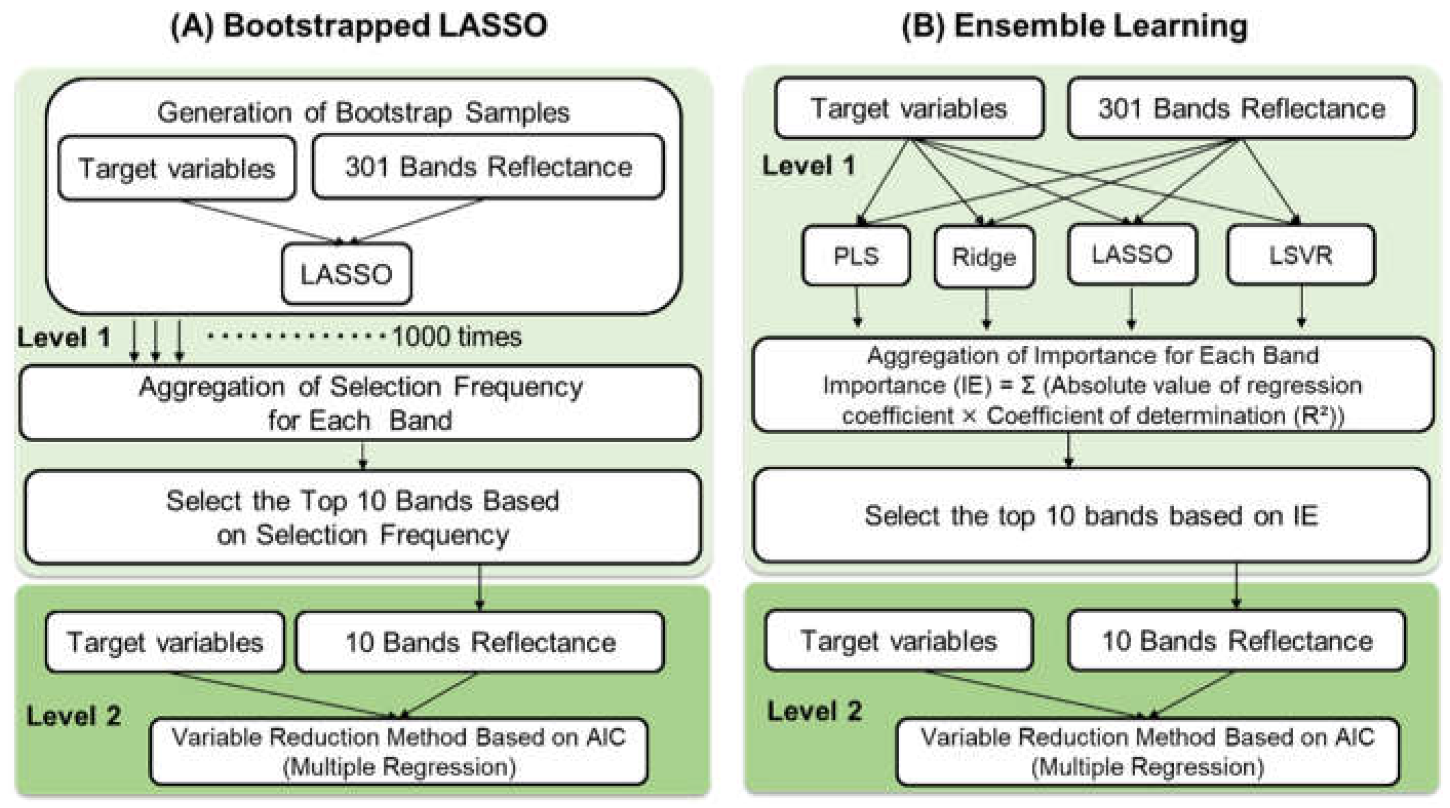
Figure 2.
Mean spectral reflectance associated with aboveground biomass (AGB) across the visible to near infrared range (501–801 nm).
Figure 2.
Mean spectral reflectance associated with aboveground biomass (AGB) across the visible to near infrared range (501–801 nm).
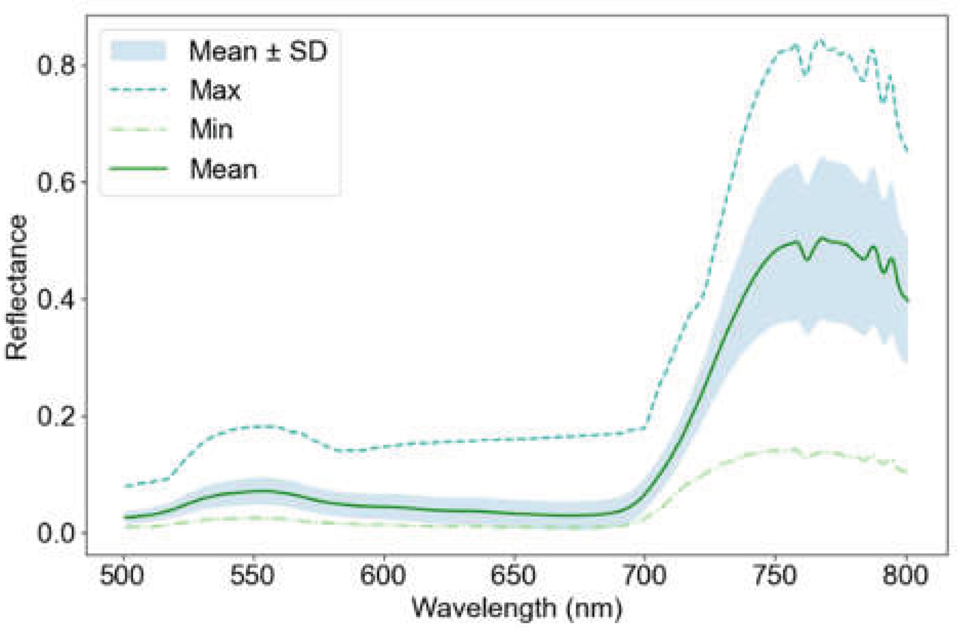

Table 1.
Descriptive statistics for soybean traits (aboveground biomass, AGB; leaf area index, LAI; and canopy cover, CC) obtained across multiple years, sites, growth stages, and cultivars.
Table 1.
Descriptive statistics for soybean traits (aboveground biomass, AGB; leaf area index, LAI; and canopy cover, CC) obtained across multiple years, sites, growth stages, and cultivars.
|
Target variables |
Mean | Max | Min | SD | CV |
| AGB (g m-2) | 374 | 1188 | 8 | 275 | 74 |
| LAI (m2 m-2) | 3.80 | 8.65 | 0.26 | 2.03 | 53 |
| CC (%) | 82 | 100 | 5 | 23 | 28 |
Table 2.
Performance of regression models for predicting aboveground biomass (AGB) using spectral reflectance data in the validation dataset, and the corresponding selected bands.
Table 2.
Performance of regression models for predicting aboveground biomass (AGB) using spectral reflectance data in the validation dataset, and the corresponding selected bands.
| Methods | PLS | PLS-VIP | BoLASSO | Ensemble |
| R2 | 0.786 | 0.369 | 0.697 | 0.604 |
| nRMSE (%) | 28.8 | 49.5 | 34.3 | 39.3 |
| Number of explanatory variables | 301 | 6 | 8 | 8 |
| Selected bands (nm) | All bands | 677, 680, 683, 762, 793, 797 |
520, 525, 607, 692, 695, 716, 739, 793 | 520, 594, 606, 607, 683, 716, 792, 793 |
Model performance was evaluated using the coefficient of determination (R²) and normalized root mean square error (nRMSE, %). The number of variables indicates the final number of explanatory variables retained after variable selection. For PLS, all available bands (301 variables) were used. For PLS-VIP, BoLASSO, and the ensemble method, a subset of bands was selected based on each method and further refined using stepwise regression based on the Akaike information criterion (AIC).
Table 3.
Performance of regression models for predicting leaf area index (LAI) using spectral reflectance data in the validation dataset, and the corresponding selected bands.
Table 3.
Performance of regression models for predicting leaf area index (LAI) using spectral reflectance data in the validation dataset, and the corresponding selected bands.
| Methods | PLS | PLS-VIP | BoLASSO | Ensemble |
| R2 | 0.823 | 0.736 | 0.828 | 0.795 |
| nRMSE (%) | 21.8 | 26.5 | 21.4 | 23.4 |
| Number of explanatory variables | 301 | 7 | 6 | 6 |
| Selected bands (nm) | All bands | 502, 762, 786, 793, 796, 797, 798 | 501, 504, 704, 732, 793, 796 |
501, 704, 727, 732, 785, 786 |
See Table 2 for definitions of R², nRMSE, and the number of variables, and for details of variable selection.
Table 4.
Performance of regression models for predicting canopy cover (CC) using spectral reflectance data in the validation dataset, and the corresponding selected bands.
Table 4.
Performance of regression models for predicting canopy cover (CC) using spectral reflectance data in the validation dataset, and the corresponding selected bands.
| Methods | PLS | PLS-VIP | BoLASSO | Ensemble |
| R2 | 0.893 | 0.630 | 0.894 | 0.843 |
| nRMSE (%) | 7.7 | 14.4 | 7.7 | 9.3 |
| Number of explanatory variables | 301 | 5 | 9 | 6 |
| Selected bands (nm) | All bands | 763, 764, 793, 797, 798 | 549, 599, 610, 683, 694, 720, 724, 762, 793 | 535, 599, 683, 720, 762, 797 |
See Table 2 for definitions of R², nRMSE, and the number of variables, and for details of variable selection.
Disclaimer/Publisher’s Note: The statements, opinions and data contained in all publications are solely those of the individual author(s) and contributor(s) and not of MDPI and/or the editor(s). MDPI and/or the editor(s) disclaim responsibility for any injury to people or property resulting from any ideas, methods, instructions or products referred to in the content. |
© 2026 by the authors. Licensee MDPI, Basel, Switzerland. This article is an open access article distributed under the terms and conditions of the Creative Commons Attribution (CC BY) license (http://creativecommons.org/licenses/by/4.0/).
Copyright: This open access article is published under a Creative Commons CC BY 4.0 license, which permit the free download, distribution, and reuse, provided that the author and preprint are cited in any reuse.