Submitted:
26 May 2026
Posted:
29 May 2026
You are already at the latest version
Abstract
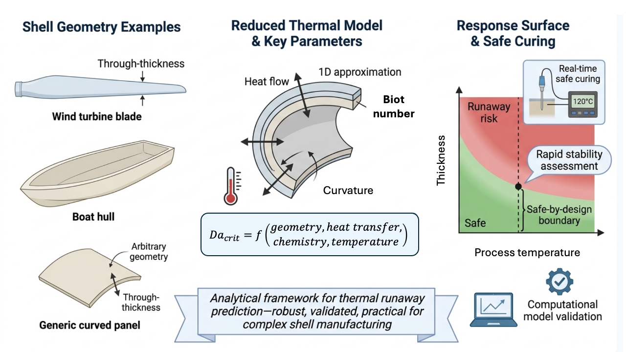
Predicting and preventing thermal runaway during cure remains a key barrier to robust process design of thick composite parts. We present an analytical framework for safe curing of thick composite shells with arbitrary geometry. By mapping the 3D thermal-kinetic problem to a locally one-dimensional through-thickness model evaluated point-wise over the shell surface, we derive a closed-form stability criterion expressed by a critical Damköhler number. The criterion reveals a clean separation between (i) a geometry/heat-transfer factor depending on local principal curvatures and Biot numbers, and (ii) a chemistry/temperature factor governed by Arrhenius sensitivity and processing temperature. The geometric stability limit is obtained from a nonlinear boundary-value problem and represented by compact response surfaces for symmetric and asymmetric boundary conditions. The model is validated against high-precision transient simulations and a quasi-three-dimensional flux assessment, confirming that transverse gradients dominate for industrially relevant curvatures. The resulting formulas provide rapid stability sweeps across complex 3D geometries, estimation of safe thickness, and provide a basis for process monitoring using temperature derivatives.
Keywords:
thermal runaway
; composite curing
; thick composite laminates
; shell structures
; composite pipes
; stability criterion
; perturbation analysis
; damköhler number
; biot number
; process design
1. Introduction
The curing of thick fibre-reinforced polymer laminates (FRP) is challenging due to the strong exothermic nature of thermoset cross-linking together with the low thermal conductivity of polymer composites. When the heat generated by the curing reaction cannot be dissipated efficiently, large temperature gradients can develop within the laminate. These gradients may lead to a heterogeneous degree of cure, accumulation of residual stresses, matrix degradation, or even delamination. During cure, chemical shrinkage and modulus development further induce residual stresses and warpage [1], which in turn can initiate transverse cracking and delamination [2]. Thermal control is therefore essential for both dimensional stability and structural integrity.
Industrial cure cycles are commonly developed on the basis of experience with thin laminates, where heat removal is relatively effective and strong temperature gradients do not arise. However, as laminate thickness increases or when rapid cure cycles are employed, the balance between heat generation and heat dissipation may be disrupted. Under such conditions, manufacturers rely on numerical simulations to predict thermal behaviour during curing. Fully coupled thermal-kinetic models, typically solved using finite-difference, finite-volume, or finite-element methods, can reproduce thermal gradients and overshoot for a wide range of composite systems [3,4,5,6]. Although these models are accurate and versatile, they can take a lot of time to apply in practice, be sensitive to the uncertainty of the kinetic parameters, and offer limited physical insight into the stability boundary that separates safe processing from thermal runaway.
Analytical approaches can provide additional insight by revealing the underlying physics and yielding explicit relations between overheating, material parameters, and geometry. However, analytical predictions of thermal runaway in composite curing remain limited. Previous work established a perturbation-based runaway criterion for flat laminates [7]. Farjas et al. [8] obtained analytical critical-thickness conditions for planar geometries with convective boundaries. In parallel, process-orientated studies [6,9] have used these flat-plate criteria to define safe operating windows in advanced manufacturing strategies. Yet, no analytical framework currently generalises these criteria to curved shells or expresses the critical condition in a form that separates geometric/boundary effects from chemistry/temperature sensitivity.
In this work, we derive a stability criterion for thermal runaway during the cure of thick composite shells by reducing the full 3D thermo-kinetic problem to a locally one-dimensional through-thickness model evaluated pointwise over the shell surface. This reduction yields a closed-form critical condition for the Damköhler number in which geometry and boundary heat transfer enter only through a single stability factor, while chemistry and processing temperature enter through an explicit Arrhenius scaling. We compute the geometric stability factor from a nonlinear boundary-value problem and represent it by compact response surfaces for symmetric and asymmetric Robin boundary conditions, allowing rapid stability mapping over arbitrary shell geometries and Biot numbers. We validate the resulting criterion against high-precision transient simulations and a quasi-three-dimensional flux assessment, which confirms that transverse gradients dominate for industrially relevant curvatures and that the locally 1D approximation is conservative. Finally, we introduce an objective numerical classification of runaway onset based on temperature derivatives, providing a consistent way to locate the critical threshold in transient simulations and suggesting a route to real-time process monitoring.
The paper is organised as follows. Section 2 formulates the locally 1D shell model, introduces the perturbation framework, and derives the stability condition and its parameter separation. Section 3 validates the criterion against fully coupled transient simulations and examines the transient behaviour near criticality. Section 4 discusses the implications for process design and the limits of the underlying assumptions. Appendices A and B provide the derivation details and numerical procedures, respectively.
2. Theory and Numerical Methods
We formulate the governing thermo-kinetic problem for a general thick-walled shell in body-fitted coordinates and derive a thermal-runaway stability criterion. The formulation starts from the full three-dimensional energy balance with standard cure kinetics, which makes the geometric scope explicit: locally, any smooth shell is characterised by its two principal curvatures. We then introduce a controlled reduction to a locally one-dimensional through-thickness model, yielding a conservative stability problem that can be evaluated pointwise over the surface. Details of the perturbation derivation are given in Appendix A; numerical procedures are summarised here and documented in Appendix B.
2.1. Problem Formulation
The theory was developed for a general curved shell of half-thickness w whose mid-surface is described by two principal curvatures and . A body-fitted coordinate system is defined with orthogonal principal-curvature coordinates on the mid-surface and a thickness coordinate z that measures the distance from the mid-surface along the surface normal (see Figure 1). Any point in the laminate can be expressed as
where .
Since the goal is to develop a theory that is valid for shells with arbitrary shape, the analysis will start from the most general formulation of the energy conservation equation combined with a standard autocatalytic cure kinetic model [10]:
where T is the temperature, is the degree of cure, is the anisotropic thermal conductivity tensor and all other parameters have their standard meaning (see e.g. [7]).
The general problem has no known analytical solution, but it can be reduced to a one-dimensional equation along the thickness direction if in-plane conduction is neglected. In-plane conduction mainly redistributes heat laterally and therefore acts as a stabilising mechanism with respect to the risk of thermal runaway. Neglecting in-plane conduction thus yields a conservative (worst-case) approximation in which each surface point behaves as an independent through-thickness "thermal pillar". Crucially, because these thermal pillars are decoupled from their surroundings and depend strictly on the local principal curvatures, this single 1D formulation remains valid for every point on any smooth geometric shape. This decoupling allows the critical limit for thermal runaway to be precomputed over a broad range of curvatures and represented by compact response surfaces for rapid stability mapping on complex geometries.
Under this assumption, and using standard differential-geometry identities for orthogonal surface coordinates with principal curvatures and , the energy equation (1) reduces to
where is the transverse (through-thickness) conductivity associated with . To accommodate heated tooling, convection heating, or insulating boundaries within a unified mathematical framework, a Robin (convective) boundary condition is applied on both surfaces:
where n is the outward unit normal, is the heat transfer coefficient, is the reference temperature in Newton’s law of cooling [11] and is the temperature at the surface of the part.
To reveal the governing non-dimensional groups and reduce the total number of independent process parameters, all variables are scaled using the same procedure as in [7]:
- through-thickness coordinate scaled with the laminate half-thickness ,
- time with the thermal-diffusion time from the boundary to the centreline ,
- temperature with the adiabatic temperature rise ,
- and curvature with the thickness .
With these scalings, the governing equations take the dimensionless form:
with dimensionless boundary conditions
where the Damköhler number , the Arrhenius number and the Biot numbers are defined as:
2.2. Perturbation Solution
From this point onwards, the tilde notation is dropped and all variables are dimensionless unless otherwise stated.
To make the coupled thermal–kinetic problem tractable, two simplifying steps are introduced (see Appendix A for details).
First, the kinetic term is frozen at its maximum value, replacing
with a constant, . This corresponds to the most heat-intensive stage of cure and therefore yields a conservative (worst-case) approximation of the runaway risk. With this approximation, the heat-generation term no longer depends on the evolving degree of cure, which decouples the energy equation from the cure kinetics.
Second, the analysis focuses on the steady-state temperature distribution that would arise if the laminate was exposed to its highest admissible background temperature . If the part can reject reaction heat under these conditions, it will remain stable through the transient leading up to the stationary state. The temperature is therefore written as a small correction to this reference state,
which leads to a static through-thickness problem for the perturbation temperature profile (see Appendix A):
Here the dimensionless parameter
measures the balance between heat generation and heat removal.
The corresponding boundary conditions involve only the Biot numbers and are independent of the reference temperature , a direct consequence of expanding the temperature field around this reference state:
The perturbation problem admits a steady solution only if is below a certain threshold. When exceeds this limit, the steady-state temperature profile can no longer exist and the temperature becomes self-accelerating. Because the parameters governing the perturbation equation are the curvatures and the Biot numbers , the critical value
is determined entirely by geometry and surface heat transfer.
Once is known, the corresponding critical Damköhler number follows directly from Equation (9):
This expression separates the effects of geometry and heat transfer (contained in ) from those of chemistry and processing temperature. The critical Damköhler number can be recast as a criterion for the maximum safe half-thickness of the laminate for given process conditions:
The perturbation BVP in Equation (8) is still too complicated to solve analytically. However, a semi-analytical solution can be developed by solving the BVP numerically for a range of curvatures and Biot numbers and fitting an analytical expression to the numerical results. The determination of for each parameter set is done by an iterative search for the upper limit for valid solutions to the stationary problem (see Appendix B for details). The resulting map of versus curvatures and Biot numbers is used to fit analytical expressions. The resulting semi-analytical result can then be used as the basis for the universal thermal runaway criterion.
The perturbation solution also predicts the peak temperature rise at the stability limit:
where is an shape factor that only depends on .
For a flat laminate with Dirichlet boundary conditions [7]. However, for other curvatures, it is difficult to determine accurately from the BVP because even a very small uncertainty in is strongly amplified in the peak-temperature estimate. This sensitivity makes the stepping method used to locate (see Appendix B) poorly suited for extracting directly from the perturbation equation.
Instead, the peak temperature at critical conditions is obtained from the full transient numerical model described in Appendix B, which exhibits much weaker sensitivity to small errors in the critical limit. The resulting values of are then fitted to the analytical scaling law above, ensuring consistency between the perturbation theory and the exact numerical solution.
In summary, the perturbation method offers an intuitive description of thermal-runaway onset: geometry and surface heat transfer determine the shape of the stability boundary, while chemistry influences the critical Damköhler number through a simple exponential dependence. The resulting stability criterion in Equation (10) is concise, physically transparent, and highly accurate, as confirmed by comparison with fully coupled numerical simulations in the Results section.
The discussion that follows examines the shape of the surface for two practically important heating configurations: (i) symmetric heating, where both surfaces have the same Biot number, and (ii) asymmetric heating, where one surface is strongly coupled to the surroundings and the other has a variable heat-transfer coefficient. These two cases cover the vast majority of industrial curing setups and illustrate the essential trends in how curvature and boundary conditions influence stability.
2.2.1. Symmetric Heating
Figure 2 shows the stability surface for the case of symmetric heating, here illustrated with . Changing the Biot number shifts the overall height of the surface but does not alter its geometric shape. What is immediately apparent is the symmetry about the diagonal . This reflects the exchange symmetry of the governing equations: interchanging the principal curvatures does not change the physical problem, and therefore .
A second symmetry appears along the opposite diagonal, where . Under symmetric heating, flipping both curvatures simultaneously and changing the direction of the thickness coordinate x corresponds to reversing the shell orientation while leaving the heat-transfer conditions unchanged. Because the perturbation equation depends on the curvatures only through the combination the stability limit is unaffected by this transformation. Together, these two symmetries explain the characteristic appearance of the stability surface in Figure 2.
These symmetries strongly constrain the functional form of any analytical expression for . By rewriting the surface in terms of the curvature invariants and , both symmetry conditions are satisfied automatically. This makes it possible to approximate the entire stability surface using a compact polynomial in S and P, which closely reproduces the numerical data:
The coefficients and are obtained from a least-squares fit to the numerical data. While these parameters exhibit a weak -dependency for low Biot numbers , they are treated here as constants to maintain the analytical simplicity of the universal criterion. For typical laminate curvatures , this approximation introduces an error of less than 1% for , and remains highly accurate even at with a maximum error of approximately 2.2%. Consequently, the curvature effects are decoupled from the surface heat transfer in the model, and only the offset term is required to vary with :
where is a fitting parameter. The reference value represents the analytical stability limit for a flat slab under Dirichlet boundary conditions [7]. Equation (13) captures the dominant -dependence with high fidelity, reflecting the rapid boundary-layer saturation observed as the process moves toward a diffusion-limited regime (see Figure 3).
Taken together, the symmetric-heating results provide a clear physical picture of how geometry and heat-transfer conditions influence the onset of thermal runaway. Increasing curvature consistently lowers the stability margin: as the shell becomes more curved, heat is removed less efficiently through the thickness, so runaway occurs under milder chemical conditions, embodied by the Arrhenius number and the processing temperature . In contrast, the Biot number affects the overall sensitivity more directly and independently of curvature; a larger Biot number simply means better heat transfer at the surfaces, raising the entire stability surface uniformly. The predicted peak temperature at the stability limit shows only a weak dependence on curvature but is strongly governed by the small parameter , and thus by the Arrhenius number and .
Beyond these points, several additional conclusions might be of practical interest to engineers. First, the symmetric case highlights that geometric effects act primarily as a penalty, not as a source of interaction: synclastic (dome-like) and anticlastic (saddle-like) curvatures follow the same general trends, meaning the stability limit can be characterised using only the scalar invariants S and P. Second, the rapid saturation of shows that improving surface heat transfer beyond a moderate Biot number yields diminishing returns, an important observation for tooling and process design where changes in convection or tool contact may be costly. Third, the smoothness and symmetry of the surface imply that manufacturing tolerances in curvature are unlikely to produce abrupt stability changes; instead, stability degrades gradually as curvature increases, which improves predictability in engineering assessments. Finally, the weak curvature dependence of means that temperature overshoot predictions can be made with reasonable confidence even before curvature-specific calibration, whereas safe-thickness predictions require using the full stability surface.
These conclusions together provide engineers with an intuitive and practically useful understanding of how geometry and heat-transfer efficiency shape the stability limits for thick composite shells under symmetric heating conditions.
2.2.2. Asymmetric Heating
For asymmetric heating conditions, where one surface is cooled more efficiently than the other , the coordinate-flip symmetry of the system is broken. In the symmetric case, the stability limit was invariant under the simultaneous transformation of reversing the thickness coordinate and flipping the signs of the principal curvatures . In the asymmetric case, however, this transformation is no longer a symmetry of the problem because it swaps the positions of the well-cooled and poorly-cooled surfaces relative to the direction of curvature.
Consequently, the stability limit becomes sensitive to whether the laminate is curving "towards" or "away from" the side with inferior heat extraction. This manifests as a distinct "tilt" and distortion of the stability surface (see Figure 4), particularly at low Biot numbers (Bi<10). In this regime, the onset of thermal runaway depends strongly on the orientation of the shell relative to the thermal bottleneck at the less-cooled surface. As the cooling efficiency increases toward , this sensitivity to orientation diminishes, and the stability surface eventually recovers the symmetric characteristics of the limit.
To capture this physical distortion mathematically, the semi-analytical fitting polynomial must be modified. Specifically, an additional linear term in the curvature sum S is required to account for the first-order sensitivity to curvature direction that appears when the cooling is unbalanced:
In this asymmetric regime, all four coefficients exhibit a dependency on the Biot number. The linear coefficient explicitly quantifies the "tilt" of the surface, while the remaining terms describe the evolution of the surface height and curvature sensitivity. These dependencies are accurately captured by the following fitting functions:
with the optimised coefficients listed in Table 1. These functions reproduce the surface for all fitted data with errors well below one percent (see Figure 5).
The asymmetric-heating results reveal several important differences compared to the symmetric case. The most prominent is that unequal boundary conditions introduce a directional bias into the heat-removal capability of the shell. This appears as a characteristic “tilt” of the stability surface, captured by the coefficient , which shifts the stability margin depending on whether the dominant curvature faces the hotter or the better-cooled surface. For engineers, this has a clear implication: orientation of the heating matters. A curved part with one side poorly cooled is inherently more vulnerable to runaway when its convex face is exposed to the weaker boundary condition.
Despite this asymmetry, many trends remain consistent. Mean curvature and Gaussian curvature still control the overall penalty through the coefficients and , and these vary smoothly with . Once the poorly cooled face reaches moderate heat-transfer efficiency, the influence of asymmetry decreases rapidly, mirroring the saturation behaviour discussed above. This means that in many practical setups, especially autoclave or oven curing where one surface is strongly coupled to the environment, only modest improvements to the weaker surface are needed to bring the system close to the more stable symmetric-heating case.
Another valuable insight is that the asymmetric case does not introduce any abrupt or unexpected behaviours: the stability surface remains smooth, monotonic, and predictable across the domain. Thus, while asymmetric heating reduces the overall stability margin, it does so in a way that is systematic and quantifiable, enabling engineers to evaluate the effect of tooling contact, insulation, layup orientation, and part placement without resorting to full numerical simulations. In all, the asymmetric-heating analysis completes the picture by showing how unequal boundary conditions shift, but do not fundamentally change, the underlying geometric structure of the thermal-runaway limit.
2.2.3. General Boundary Conditions
While the symmetric and strongly asymmetric configurations discussed above capture the essential physical phenomena, a general heating scenario may involve two arbitrary, unequal Biot numbers. Conceptually, the stability surface for such a general case can be understood through a superposition of the two established behaviors. If one initially assumes a symmetric state based on the higher of the two Biot numbers, the overall elevation of the surface is correspondingly reduced. Subsequently reducing the remaining surface’s Biot number to its true, lower value breaks the symmetry, introducing the characteristic "tilt" and, at sufficiently low values, the flattening observed in the asymmetric case.
Rather than developing an exhaustive semi-analytical formulation for all possible combinations, a computational approach is recommended for general conditions. The software provided in the supplementary material (detailed in Appendix B) allows the user to input any arbitrary pair of Biot numbers to automatically generate a custom polynomial fit for . Once this specific fit is generated, the thermal stability of the part can be straightforwardly evaluated using the theoretical framework established in the preceding sections.
2.3. Numerical Methods (Summary)
The perturbation boundary-value problem for is solved using MATLAB’s bvp4c with a continuation strategy in (details in Appendix B). The fully coupled transient 1D thermo-kinetic model used for validation of the perturbation model is discretized by a second-order cell-centered finite-volume method (method of lines) and integrated with MATLAB’s ode15s using a relative tolerance of (Appendix B). A grid-convergence study with Richardson extrapolation indicates that the production grid yields relative errors below for the peak temperature. Thermal runaway in the numerical solution is classified objectively using the sign of the peak second time derivative of a virtual sensor temperature at the hottest node, and is located using MATLAB’s fzero solver (Appendix B). The complete MATLAB (R2025a) source code used to generate the results is provided as supplementary material.
3. Results
This section validates the perturbation-based predictions against high-precision numerical solutions of the fully coupled thermal-kinetic problem (Eqs. 4 - 5). The standalone transient solver (Appendix B) resolves the through-thickness energy balance with Robin boundary conditions and autocatalytic kinetics without the simplifying assumptions used in the perturbation analysis. A grid-convergence study with Richardson extrapolation showed that, for control volumes, the relative error was below . The MATLAB source code used to generate all results is provided as supplementary material.
An objective classification scheme (Appendix B) was used to distinguish sub-critical from super-critical solutions based on the temperature-time history at an internal sensor point. Coupled with a bracketed search in the Damköhler number, this made it possible to determine the critical Damköhler number for any prescribed set of parameters. These “exact-solution” results are compared with the semi-analytical perturbation predictions, focusing on three aspects: (i) the geometric scaling through , (ii) the Arrhenius/temperature scaling in the prefactor, and (iii) the predicted peak temperature at criticality.
The remainder of the section is organised as follows:
(i) Characteristics of the transient temperature: Detailed study of the transient behaviour near critical conditions and how it depends on the Arrhenius number;
(ii) Geometrical validation: comparison of the numerically determined with the surface and its polynomial fit;
(iii) Chemical/temperature validation: calibration of the kinetic factor and assessment of the Arrhenius/processing-temperature scaling;
(iv) Generalisation across kinetics: extension to a wider range of kinetic exponents and evaluation of model robustness.
3.1. Characteristics of the Temperature History at Critical Conditions
When the Damköhler number exceeds its critical value, the reaction becomes self-accelerating. However, the qualitative nature of the resulting temperature rise is dependent on the Arrhenius number , which dictates whether the runaway is "mild" or "explosive."
- Mild (gradual) runaway - low: For Arrhenius numbers below a practical threshold, defined here bythe peak temperature increases gradually with , exhibiting a nearly linear dependence on up to and beyond the stability limit (see in Figure 6). In this regime, crossing does not trigger a catastrophic jump but rather a manageable increase in the exotherm.
- Ignition-like (explosive) runaway - high : For Arrhenius numbers exceeding the threshold in Equation (16), the system behaviour changes character. Sub-critical cases remain stable, but once is reached the system exhibits a long induction period followed by a rapid temperature rise toward the adiabatic limit (see in Figure 7), a behaviour closely resembling ignition in combustible mixtures [12].
At the critical limit (), the numerical peak temperature rise follows the scaling predicted by the perturbation analysis. For the cases illustrated in Figure 6 (), the numerical peak values at critical condition are approximately and , respectively. These values are slightly lower than the absolute peaks predicted by the perturbation analysis, but the ratios of the magnitudes are consistent with the theory.
The higher peak temperatures in the perturbation model compared to the numerical simulations stem from the simplified kinetics used in the perturbation model, specifically the replacement of the kinetic function by a constant, which overestimates the reaction rate throughout the cure. By neglecting reactant consumption and the specific -order kinetics, perturbation theory provides a conservative upper bound for the temperature rise. In contrast, the numerical model captures the reduction in reaction rate as conversion increases, leading to the slightly lower peak temperatures observed here.
The threshold in Eq. (16) represents a Semenov-type criterion [12] adapted to the current shell geometry and boundary conditions. Its approximate numerical value was determined by identifying the lowest at which the vs. response transitions from a continuous curve to a nearly discontinuous jump when exceeding . Although classical Semenov theory is derived for lumped systems, this empirically calibrated form successfully captures the observed bifurcation in behaviour, explaining why minor process variations in can be benign at low but catastrophic at high .
3.2. Validation of the Curvature-Chemistry Separation
The validation of the separation of curvature effects from the chemistry was done with a fixed chemistry, , taken from a reported epoxy system [4]. Anchoring the study to a documented material avoids unphysical parameter combinations. This choice does not bias the geometric results because is independent of chemistry; chemical effects enter only when converting to .
In what follows, the geometry-Biot dependence of the stability limit is taken directly from the polynomial fits in Eqs. (12) and (14) from Section 2. The resulting global stability limit defined by Equation (10) was fitted to the numerical results for the different heating options using the kinetic scaling factor as the only fitting parameter.
We first consider symmetric heating at a high Biot number (). Figure 8 shows the numerically computed stability surface . The surface exhibits the same symmetries as the surface from the perturbation analysis, namely invariance under exchange and, under symmetric boundary conditions, invariance under the combined transformation . The one-parameter fit yields , about 50% of for the chosen kinetics, indicating that the conservative choice in the Theory section is unnecessarily strict. The RMS relative error for the fit is 1.8% with a maximum deviation of 4.6% over the whole -plane.
For the moderate-convection case , the same one-parameter fitting procedure yields an almost identical coefficient, , with an RMS relative error of 2.4% and a maximum deviation of 6.4%. The closeness of to the high-Bi fit () confirms that the chemistry/process scaling is effectively independent of surface heat-transfer strength, while the Biot number acts primarily through the geometry–boundary factor (i.e., a uniform vertical shift of the surface without altering its shape). In other words, even away from the near-Dirichlet limit, the predicted separation of from holds: the semi-analytical surface from the perturbation solution can be used as is, and a single brings the model into close agreement with the full numerical results.
For asymmetric heating, the outer surface is taken nearly isothermal while the inner surface has finite thermal resistance . The computed stability surfaces again exhibit the symmetries predicted by the perturbation analysis, including the expected tilt along the mean-curvature direction for small . The semi-analytical surface from the perturbation analysis is kept unchanged and only the single kinetic factor is fitted for each . The fitted values lie in a narrow band over , while the errors decrease rapidly as increases (Table 2). The nominally “worst” case is the perfectly insulated side , where the RMS relative error is 11.6% and the maximum deviation 55.9%. However, this seemingly large error is misleading as a diagnostic: for the span of over the curvature grid exceeds one decade, so uniform absolute errors translate into larger percent errors at the low end. Consistent with this, the parity plot for is among the tightest, points cluster closely around the line across the full range (see Figure 9). Overall, the results confirm that the geometry–boundary contribution can be taken directly from the perturbation BVP, while the chemistry–temperature influence is captured by a single scalar (here ) without re-tuning the geometric fit.
Across all symmetric and asymmetric cases, the best-fit remains nearly constant () over the entire grid and Biot-number range, reinforcing that geometry/boundary effects are captured by while chemistry is well represented by a single scalar .
3.3. Chemical/Temperature Calibration
Having confirmed that the surface curvature and boundary heating dependence of the stability limit is fully captured by the perturbation theory parameter , we now turn to the calibration of the chemical prefactor . This factor represents the effective exothermic strength of the reaction and appears multiplicatively in the closed form criterion for the critical Damköhler number. The objective of this section is to determine whether a single constant value of is sufficient to represent the chemical contribution across a broad range of Arrhenius numbers and surface temperatures.
3.3.1. Calibration over and
To isolate chemical effects from geometry and boundary conditions, all calibration simulations were performed for a fixed configuration: vanishing curvature , symmetric heating with , and fixed kinetic exponents , identical to those used in the geometrical validation. The validated separation between geometry–heating intensity and chemistry–temperature ensures that this restriction does not bias the calibration.
The calibration spanned a rectangular domain in the plane, , subject to two constraints: (i) , ensuring the perturbation solution remains accurate, and (ii) exclusion of the region , where the system is prone to a sudden, catastrophic jump in temperature and severe overheating for even small excursions above . The resulting admissible domain is shown in Figure 10.
Within the calibration domain, the critical Damköhler number was extracted from fully coupled transient simulations using the objective classification scheme of Appendix B. These numerical “truth” values were then compared with the perturbation-theory prediction. A least-squares fit over the entire region gives , slightly larger than the value obtained in the geometrical study (). The fitted constant represents approximately 59% of for these kinetics and yields an average relative error of 20.5% in . Figure 11 shows that, despite the moderate absolute error, the shape of the isolines and the combined Arrhenius–temperature scaling are reproduced extremely well. A similar fitting procedure was applied to the predicted peak temperature at criticality, yielding an optimal temperature-scaling factor , with an average relative error of approximately 9.5%. As illustrated in Figure 12, the critical-temperature isolines align closely with those of constant in Figure 10, consistent with the theoretical structure of the perturbation solution.
Overall, the comparison demonstrates that the semi-analytical perturbation framework captures the dominant chemical and thermal scaling across a broad parameter space. The fitted constants and are effectively uniform over the calibration domain, and the remaining discrepancies are of the magnitude anticipated for a first-order perturbation approximation. Most importantly, the isoline alignment confirms that the perturbation solution retains the correct topology of the stability boundary, validating its use as a reduced-order predictive model for thermal runaway.
3.4. Generalisation Across Kinetics
Autocatalytic reaction models of the form are widely used to describe thermoset curing [10]. However, only a restricted subset of exponent pairs produces conversion-rate profiles that resemble experimentally observed behaviour. In particular, very small values of m or unusually large values of n cause the reaction rate to become highly skewed: the peak of shifts unrealistically close to either or , the maximum value becomes excessively sharp, and the overall curve loses the broad, single-hump shape characteristic of epoxy and polyester systems. Such behaviours are inconsistent with DSC measurements reported in the literature and lead to runaway thresholds that do not represent industrial thermosets.
To ensure physically meaningful kinetics while still covering a broad range of autocatalytic behaviours, we therefore restrict attention to
a domain consistent with reported kinetic fits for common resin families and free from pathological rate-curve shapes. Within this region, remains single-peaked, moderately skewed, and shows the characteristic early-stage acceleration followed by depletion-driven decay. Most commercial resin systems fall well within this window, and the associated rate curves differ primarily in width and skewness rather than in qualitative shape. Should values outside this region be required, a new calibration can easily be performed using the software provided in the supplementary material.
Dense Sweep and Global Response-Surface Fit
A full systematic sweep across the domain was carried out to obtain a smooth functional form for . Each pair was calibrated against a dense grid in , yielding a corresponding value of that was used to define a damping factor that relates to the maximum of the kinetic function:
where . The sweep used a grid in and, for each point, a grid in , with the fitting procedure for identical to that used for the chemical calibration.
The resulting optimised parameters and , their associated relative errors for and , and the normalised damping factor
are summarised in Table 3. The consistency of and across these widely separated kinetic exponents confirms that the calibration procedure is consistent across the parameter range.
The resulting data were fitted to a low-dimensional polynomial response surface:
with coefficients
yielding .
A similar fit was obtained for the temperature-scaling factor:
with
and .
Final Predictive Forms
For operational use, the effective rate constant is taken as
with
Within the calibration region
subject to the constraint and excluding the folded S-curve regime, the damping factor remains bounded between and . Outside this region, K should be taken as capped at , corresponding to the limiting case , which is guaranteed to yield a critical limit on the safe side of the value obtained from the exact solution.
Temperature-Rise Generalisation
An analogous generalisation applies to the maximum temperature rise at . As shown in Table 3, the factor varies systematically with , ranging from approximately to . These variations are consistent with perturbation-theory expectations: changes in the skewness of alter the heat-release rate, but remains across all practical cases. The relative error in remained between and across all tested exponent pairs.
Fitting the numerical data to provides a smooth functional dependence that reproduces numerical calibrations with high fidelity. Although the model could theoretically be refined by incorporating explicit semi-analytical corrections for local curvatures and Biot numbers , the current formulation already demonstrates excellent accuracy. Therefore, this simpler approach was retained to prioritize ease of practical implementation without compromising predictive reliability. The resulting expression for the peak temperature rise is
using the fit for from Equation 18.
3.4.1. Verification of Global Accuracy
To rigorously verify the global accuracy of the fully assembled model, a final validation series was conducted using a fractional factorial experimental design [13]. The parameter space was bounded by the limits of extreme industrial part geometries , spanning flat, strongly synclastic, and strongly anticlastic shells. Boundary conditions were restricted to either fully symmetric cooling or heavily asymmetric cooling . The kinetic exponents were tested at the boundaries of the admissible domain .
An 8-run orthogonal test matrix was constructed to sample the corners of this multidimensional space without redundant geometric configurations. For each of the 8 cases, a direct numerical calibration sweep over the plane was performed to extract the true values of and . These were then compared against the closed-form predictions of the global model. Because and , the relative errors in these prefactors directly represent the model’s predictive error for the runaway threshold and exotherm severity. The results, summarized in Table 4, demonstrate that the global equations successfully capture the compounding effects of asymmetric curvature, heat transfer, and complex kinetics.
3.5. Assessment of In-Plane Thermal Fluxes and Model Assumptions
The theoretical framework presented in Section 2 assumes that through-thickness (transverse) heat conduction is the dominant mode, allowing in-plane conduction along the shell surface to be neglected. To validate this assumption, a quasi-three-dimensional (Quasi-3D) numerical analysis was performed on a representative saddle geometry. The computational domain is discretized via a 3D finite volume mesh, constructed by extruding a body-fitted orthogonal mid-plane mesh toward the inner and outer surfaces. Temperature profiles for the resulting through-thickness "thermal pillars" are initially computed using the 1D solver established in this study. Finally, the potential in-plane fluxes are integrated over the lateral faces of each thermal pillar and compared against the total transverse flux through the pillar’s end faces. This ratio provides a quantitative measure of the 1D assumption’s validity. Detailed algorithmic implementation and the discretization scheme are provided in Appendix B, with the corresponding MATLAB source code available as supplementary material.
A critical observation in the design of shell structures is that geometries that appear highly curved may still correspond to small dimensionless curvatures because of the small thickness-to-radius ratio typical of composite laminates. While the perturbation theory in Section 2 remains mathematically valid for dimensionless curvatures up to , most practical engineering applications, including the saddle geometry in Figure 13 for which , fall well within this range.
The results of the Quasi-3D analysis, summarized in Figure 13, demonstrate that even at the onset of thermal runaway, the "worst-case" scenario for thermal gradients, the net in-plane heat flux remains orders of magnitude smaller than the transverse flux. For the saddle geometry, the maximum flux ratio was found to be , corresponding to an in-plane flux of about of the transverse flux. This negligible ratio confirms that the high aspect ratio of the laminate and the magnitude of the transverse cooling effectively decouple the thermal behavior of adjacent surface elements. Consequently, the locally 1-D universal model can be used to predict safe process parameters for complex shell geometries with high confidence, as the error introduced by neglecting in-plane conduction is significantly smaller than typical uncertainties in material properties and kinetic parameters.
To further assess the robustness of this approximation, a sensitivity analysis was performed by varying the inner-wall cooling conditions while maintaining high outer cooling . In the extreme case of a perfectly insulated inner boundary , the maximum in-plane flux ratio was . As the inner cooling is increased, the ratio exhibits a non-monotonic trend: it increases to a peak of at , then decreases and stabilizes at for . This convergence toward the symmetric cooling value is consistent with the finding in Section 2 that thermal asymmetry becomes negligible when exceeds 100. Because the omission of in-plane conduction effectively removes a potential cooling pathway, the 1-D model serves as a conservative "worst-case" predictor; it will exhibit thermal runaway slightly earlier than a full 3-D system, therefore providing an inherent safety margin for industrial process design.
4. Discussion
The Power of Dimensional Reduction and Universal Scaling. Although modern computational power enables direct numerical simulation (DNS) of thermal runaway in specific geometries, such point solutions provide limited insight into the governing physics. By reducing the problem dimensionally, the high-dimensional space of physical variables (thermal properties, kinetics, geometry, and process conditions) collapses into a small set of governing parameters . This reveals scaling laws that are otherwise obscured. In particular, stability does not depend on curvature or thickness alone, but on their dimensionless product . The resulting framework defines a universal “safe-by-design” envelope through , independent of discretisation details or solver settings.
Validity of the Locally 1-D Approximation. A central question is whether neglecting in-plane conduction introduces a significant error. Quasi-3D analysis (Section 3.5) shows that for dimensionless curvatures and aspect ratios typical of composite laminates, transverse gradients dominate the thermal response. Even under strong curvature and asymmetric boundary conditions (e.g., ), the in-plane flux remains on the order of a few percent of the total heat dissipation. This confirms that the locally 1-D formulation captures the dominant heat-transfer pathways and is not merely a mathematical simplification.
Generality across arbitrarily shaped geometries. The applicability to arbitrary shell geometries follows from the fact that any smooth surface is locally defined by its dimensionless principal curvatures, and . By expressing the problem in terms of these local invariants, the model decouples the stability criterion from global geometry. Therefore, complex structures can be analysed as collections of independent “thermal pillars”, each governed by local curvature. In practice, even visually pronounced curvature often corresponds to moderate dimensionless values , where the analytical model is most accurate.
Robustness under Asymmetric Boundary Conditions. Perfectly symmetric cooling is rare in practice, which makes asymmetric boundary conditions essential to consider. The results show that stability is strongly influenced by the better-cooled surface: even modest increases in the corresponding Biot number significantly raise the runaway threshold. This insight has direct practical implications. For example, improved convection on the accessible surface can compensate for limited tool-side heat extraction, an effect that can be quantified directly using the analytical model without resorting to full 3D simulations.
Practical Implementation for Process Design. The framework is readily applicable in engineering practice. Local principal curvatures can be extracted from standard CAD tools, after which the semi-analytical expressions are evaluated pointwise over the surface. This identifies the least stable location through the minimum , automatically capturing the reduced stability of anticlastic regions relative to synclastic ones. Combined with estimates of Biot numbers and processing temperature, the model enables rapid assessment of safe operating conditions. If excessive peak temperature is predicted, mitigation can be achieved by increasing surface heat transfer or introducing intermediate dwell steps to reduce the accumulated reaction heat.
Consistency Between Dynamic Detection and Perturbation Theory. The second-derivative criterion aligns closely with the perturbation-based stability limit. In the perturbation framework, runaway occurs when no steady temperature profile can balance heat generation and conduction. Dynamically, this same transition is detected when , marking the onset of self-acceleration. The agreement between these independent approaches demonstrates that the transient acceleration signal reflects the same underlying stability limit as the analytical theory. This provides strong support for using the second derivative as an early-warning indicator in practical applications.
Real-Time Monitoring and Active Process Control. The second-derivative criterion used to classify the numerical solutions also provides a practical basis for real-time process monitoring. During stable curing, heat removal dominates and the temperature response is decelerating . If starts increasing and approaches zero from the negative side, the system reaches a critical balance where heat generation begins to exceed cooling capacity. This transition is detectable before large temperature rises occur. Monitoring the curvature of the temperature signal therefore provides an early-warning indicator and enables timely intervention, for example by reducing the tool temperature or introducing a temporary dwell. In this way, the tooling can act as an active control element rather than a passive thermal boundary.
5. Conclusions
In this work, a universal stability framework for thermal runaway during the cure of composite shells has been developed and validated. The main conclusions are:
- A unified analytical criterion. A general analytical stability criterion has been derived for arbitrary shell geometries and convective (Robin) boundary conditions. The resulting closed-form expression for the critical Damköhler number, , separates the influence of geometry and heat transfer from that of chemistry and processing temperature. This reduces the full 3D stability problem to a single non-dimensional margin , providing a universal “safe-by-design” framework.
- Validation of the locally 1-D approximation. The central modelling assumption, that through-thickness conduction dominates over in-plane transport, was validated using a quasi-3D flux analysis. Even for curved shells and asymmetric boundary conditions, in-plane heat fluxes remain small (typically of the transverse flux). This confirms that the locally 1-D formulation accurately captures the dominant heat-transfer mechanisms and provides a conservative estimate of stability.
- Geometric scaling of stability. The analysis shows that geometric effects enter the stability problem through the dimensionless curvature , rather than curvature or thickness separately. This scaling enables direct transfer of results across different materials and part sizes, and allows complex shells to be treated as collections of independent local “thermal pillars” governed by principal curvatures.
- Arrhenius-dependent runaway behaviour. The nature of thermal runaway is governed by the Arrhenius number . Low leads to gradual, mild transitions, while high produces ignition-like behaviour with long induction periods followed by rapid temperature rise. The analytical framework captures the stability limit in both regimes, providing guidance on whether process deviations are likely to be manageable or catastrophic.
- Role of boundary conditions and tooling. Boundary heat transfer has a dominant influence on stability, particularly under asymmetric conditions. The results show that the better-cooled surface controls the stability margin, implying that improvements in accessible surfaces (e.g. enhanced convection) can compensate for poor cooling elsewhere. This highlights the dual role of tooling as both a heat source and a heat sink.
- Practical applicability and implementation. The semi-analytical model is computationally inexpensive and can be applied directly using curvature data from CAD models and standard heat-transfer estimates. It enables rapid identification of critical locations, prediction of safe thickness, and evaluation of process modifications such as dwell steps or improved cooling strategies.
Together, these results provide a physically transparent and practically applicable framework for predicting and preventing thermal runaway in the manufacture of thick composite structures.
Supplementary Materials
The following supporting information can be downloaded at the website of this paper posted on Preprints.org.
Funding
This research received no external funding
Data Availability Statement
The MATLAB source code to all programs that were used to generate the results and figures in the paper are provided in the supplementary material file and are free to use under the GNU General Public License.
Acknowledgments
During the preparation of this manuscript, the author used Microsoft Copilot and Google Gemini for the purposes of improving language and as support in Matlab programming. The author has reviewed and edited the output and take full responsibility for the content of this publication.
Conflicts of Interest
The author declare no conflicts of interest.
Abbreviations
| Abbreviation | Meaning |
| BVP | Boundary Value Problem |
| DNS | Direct Numerical Simulation |
| FRP | Fibre-Reinforced Polymer |
| FVM | Finite Volume Method |
| ODE | Ordinary Differential Equation |
| PDE | Partial Differential Equation |
| 3D | Three-Dimensional |
| 2D | Two-Dimensional |
| Damköhler number | |
| Arrhenius number | |
| Reference temperature in the Robin boundary condition | |
| Biot number used in the Robin boundary condition. | |
| Model parameter approximating the kinetic function | |
| Adiabatic temperature rise |
Appendix A. Derivation of the Perturbation Stability Criterion
This appendix provides a concise derivation of the perturbation-based stability criterion, starting from the dimensionless energy and kinetic equations (Eqs. 4–).
Appendix A.1. Controlled Approximations
To transform the transient coupled system into a tractable stability problem, three approximations are introduced:
- 1.
-
Decoupling of kineticsThe autocatalytic factor is replaced by its maximum value , where . This produces a conservative, worst-case estimate of heat generation.
- 2.
-
Small temperature-rise expansionThe temperature field is expanded as a perturbation series about the zeroth-order solution :where is the first-order perturbation function. The dimensionless small parameter will be selected later to simplify the resulting perturbation equation.
- 3.
-
Steady-state limitAlthough the perturbation approach allows the analysis of the fully transient problem, the stability of the problem is determined by the behaviour of the solution after the initial heating phase. In the absence of internal heating, the boundary-driven temperature reaches the limit after approximately one dimensionless time unit since the scaling of time is done with the characteristic heat conduction time. If a balance between heat release and cooling by the boundaries can be maintained at this thermal maximum, it must also be valid during the preceding transient heating. The perturbation problem is therefore formulated at the steady-state limit where . The resulting perturbation ansatz therefore becomes:where the zeroth order solution has been replaced by its constant stationary solution .
Appendix A.2. The First-Order Perturbation Equation
The Arrhenius exponential in the energy equation creates a difficulty, but it can be eliminated by chosing the small parameter , which after Taylor expansion of the argument yields:
Substituting the perturbation series into the decoupled energy equation and collecting all terms yields the first-order ODE:
where the dimensionless stability parameter is:
Appendix A.3. Boundary Conditions
The dimensionless Robin conditions applied in the main text lead, at first order, to:
Equations (A2)–(A5) form a nonlinear boundary-value problem for with as a parameter.
Appendix A.4. Definition of the Critical Stability Limit
A stationary solution exists only if the heat-generation term can be balanced by conduction in the curved shell. The critical stability limit is therefore defined as the value where the solution to Equations (A2) - (A5) disappears. Because geometry and boundary conditions appear only in the differential operator and BCs, .
Appendix A.5. Peak Temperature Rise at Criticality
The first-order perturbation solution predicts a peak temperature rise at criticality of
where .
Appendix B. Detailed Numerical Procedures
This appendix outlines the numerical methods used to solve the governing equations and classify the stability of the cure cycle. To ensure full transparency and reproducibility, the complete MATLAB source code used to generate all results in this manuscript is provided in the supplementary material under the GNU General Public License (GPL).
Appendix B.1. The Perturbation Boundary-Value Problem
The geometric stability limit, , is determined by identifying the threshold value of beyond which the nonlinear boundary-value problem (Equation A2) ceases to possess a stationary solution. This is implemented using MATLAB’s bvp4c solver, which utilizes a fourth-order collocation method based on Lobatto quadrature with adaptive mesh refinement.
To ensure robust convergence, a sequential continuation strategy is employed. For every new geometric configuration, the search initializes with a “cold start” at using an analytical parabolic profile. The parameter is then incrementally increased (), utilizing the converged solution from the previous step as the initial guess for the next. The critical limit is defined as the last value of for which the solver successfully converges, guaranteeing an accuracy of .
Appendix B.2. The Fully Coupled Transient Model
The fully coupled 1D transient model is solved using the Method of Lines [14]. The spatial derivatives are discretized using a second-order, cell-centered Finite Volume Method (FVM) [15]. To maintain global second-order accuracy and prevent order reduction at the boundaries, the Robin boundary fluxes are evaluated using temperatures extrapolated to the physical walls ( and ) via a second-order one-sided stencil. The resulting system of stiff ordinary differential equations is integrated in time using MATLAB’s ode15s solver with a relative tolerance of .
A grid convergence study using Richardson extrapolation [15] on three nested grids () confirmed that the spatial discretization achieves a super-convergent order of to for the peak temperature. The estimated spatial discretization error for the production grid of nodes is verified to be below .
Appendix B.3. Quasi-3D Validation Framework
To validate the locally 1D assumption, a Quasi-3D analysis was performed by mapping the shell surface onto an orthogonal grid of local principal curvatures. The 1D transient solver is executed independently for each resulting volumetric "thermal pillar” (frustum) to generate a 3D transient temperature field, .
At the moment of maximum exotherm (), the lateral heat leakage through the East, West, North, and South faces of every layer i is calculated using a central finite difference between neighboring thermal pillars. For example, the flux through the East face of a thermal pillar at layer i is determined by the temperature gradient between the current pillar and its neighbor in the u-direction. The total lateral flux magnitude for a given thermal pillar is summed over all N layers:
The validity of the 1D approximation is quantified by the ratio of this lateral leakage to the primary transverse heat exchange at the boundaries:
A ratio confirms that transverse conduction strictly dominates the local energy balance. Detailed implementation of the geometric mapping and the face-flux calculations can be found in the computeLateralFlux.m function within the provided supplementary software.
Appendix B.4. Thermal Runaway Detection and Critical Limit Search
The transition to thermal runaway is identified by evaluating the temperature history, , at a fixed virtual sensor located at the spatial node reaching the highest absolute temperature. The stability is classified by analyzing the second derivative with respect to time ().
To isolate the chemical exotherm from the initial boundary heating, the signal is truncated for . Furthermore, the analysis window is strictly bounded at to prevent the algorithm from locking onto the asymptotic cooling phase. Within this window, a sub-critical cure is characterized by a strictly negative acceleration peak (), indicating sufficient cooling. A super-critical runaway is identified by a positive acceleration peak (), marking the onset of self-acceleration.
The critical Damköhler number, , is identified as the root of this classification function (). This is located using a robust search algorithm that first expands to establish a strict bracket spanning the sign change, followed by execution of MATLAB’s fzero routine within this bracket to resolve to a relative tolerance of .
References
- Bogetti, T.A.; Gillespie, J.W. Process-Induced Stress and Deformation in Thick-Section Thermoset Composite Laminates. Journal of Composite Materials 1992, 26, 626–660. [CrossRef]
- Rabearison, N.; Jochum, C.; Grandidier, J.C. A cure kinetics, diffusion controlled and temperature dependent, identification of the Araldite LY556 epoxy. Journal of Materials Science 2011, 46, 787–796. [CrossRef]
- Secord, T.W.; Mantell, S.C.; Stelson, K.A. Scaling analysis and a critical thickness criterion for thermosetting composites. Journal of Manufacturing Science and Engineering, Transactions of the ASME 2011, 133, 1–6. [CrossRef]
- Li, M.; Zhu, Q.; Geubelle, P.H.; Tucker, C.L. Optimal curing for thermoset matrix composites: Thermochemical considerations. Polymer Composites 2001, 22, 118–131. [CrossRef]
- Twardowski, T.; Lin, S.; Geil, P. Curing in Thick Composite Laminates: Experiment and Simulation. Journal of Composite Materials 1993, 27, 216–250. [CrossRef]
- Taddei, F.; Struzziero, G.; Michaud, V. Mitigation of infusion and cure-induced defects for thick thermosetting composites: Current challenges and future trends. Polymer Composites 2025, 46, S9–S25. [CrossRef]
- Gebart, R. Thermal runaway criterion for thick polymer composites. Composites Part A: Applied Science and Manufacturing 2024, 182. [CrossRef]
- Farjas, J.; Sanchez-Rodriguez, D.; Zaidi, S.; Cârstea, D.R.C.; Elfatah, A.M.S.A.; Rotaru, A.; Costa, J. Analytical prediction of the thermal overheating in curing thick layers of fibre-reinforced thermosets. Composites Part A: Applied Science and Manufacturing 2025, 193, 108815. [CrossRef]
- Taddei, F.; Struzziero, G.; Michaud, V. A numerical study of a tow-by-tow curing approach for residual stress mitigation in thick composites. Composites Part A: Applied Science and Manufacturing 2026, 200, 109283. [CrossRef]
- Halley, P.J.; Mackay, M.E. Chemorheology of thermosets—an overview. Polymer Engineering & Science 1996, 36, 593–609. [CrossRef]
- Incropera, F.P.; Dewitt, D.P.; Bergman, T.L.; Lavine, A.S. Principles of Heat and Mass Transfer, global ed.; John Wiley & Sons, 2017; pp. 1–978.
- Law, C.K. Combustion Physics; Cambridge University Press, 2006; pp. 1–722. [CrossRef]
- Box, G.; Hunter, J.; Hunter, W. Statistics for Experimenters, 2nd ed.; John Wiley & Sons Inc., 2005.
- Hirsch, C. Numerical Computation of Internal and External Flows; Elsevier, 2007. [CrossRef]
- Ferziger, J.; Peric, M. Computational Methods for Fluid Dynamics, 3rd editio ed.; Springer Verlag, 2013.
Figure 1.
Generic double-curved geometry with a body-fitted coordinate system with in-plane coordinates and transverse coordinate z.
Figure 1.
Generic double-curved geometry with a body-fitted coordinate system with in-plane coordinates and transverse coordinate z.

Figure 2.
Critical stability limit as a function of principal curvatures and for symmetric heating/cooling . The surface is generated over a grid in the -plane using the numerical BVP solver described in Appendix A.
Figure 2.
Critical stability limit as a function of principal curvatures and for symmetric heating/cooling . The surface is generated over a grid in the -plane using the numerical BVP solver described in Appendix A.

Figure 3.
Dependence of the offset coefficient on the Biot number for symmetric boundary conditions. The symbols are obtained from high-precision numerical solutions of the perturbation BVP, while the solid line shows a fit to the data using , where is the analytical solution for fixed temperature and is a fitting parameter.

Figure 4.
Critical stability limit as a function of principal curvatures and for asymmetric heating/cooling . The broken symmetry manifests as a tilt in the surface, which depresses the corner and lifts the corner. The surface is generated over an 11×11 grid in the -plane using the numerical BVP solver described in Appendix A.

Figure 5.
Coefficients in the polynomial for the asymmetric heating case with and variable. A complete sweep over was used to fit the coefficients for each value.
Figure 5.
Coefficients in the polynomial for the asymmetric heating case with and variable. A complete sweep over was used to fit the coefficients for each value.

Figure 6.
S-curve behavior of the peak temperature rise in a flat laminate () for , , and . The Damköhler numbers are normalized by the critical value () identified via the second derivative classification method described in the appendix. The vertical dashed line at indicates the transition beyond the stability limit into the runaway regime.

Figure 7.
Dimensionless centerline temperature evolution at high Arrhenius number . The comparison between a sub-critical () and super-critical () state demonstrates the sensitivity to small changes in the Damköhler number near the critical value and the long induction period (quiescent phase) characteristic of high thermal sensitivity.

Figure 8.
Numerically computed stability limit over the curvature plane for fixed chemical parameters , , and . Symmetric high-Biot boundary conditions () and a reference surface temperature are applied. The surface exhibits the same symmetries and geometric structure as the perturbation-theory prediction, and the theoretical model with reproduces the numerical results with an RMS relative error of 1.8% and a maximum deviation of 4.6%.

Figure 9.
Parity plot comparing numerically extracted values of from the full conduction–reaction model with the theoretical prediction obtained from the perturbation-theory stability surface. Results correspond to the asymmetric case with one side perfectly insulated (). All points from the curvature grid fall close to the ideal line, confirming excellent agreement between the full model and the analytical criterion.

Figure 10.
Calibration domain in the plane. The black curves represent iso-lines, while the red line indicates the boundary above which the system exhibits a sudden, catastrophic temperature jump for small excursions above . This highly sensitive region is excluded because it represents unsafe processing conditions that are avoided in practice. Restricting the domain below this boundary maximizes the model’s accuracy within the industrially relevant parameter space and avoids numerical ill-conditioning in the runaway detection algorithm. Finally, the region is excluded to ensure the perturbation solution remains accurate.

Figure 11.
Comparison between the numerically computed critical Damköhler number and the prediction by the perturbation theory with . The value of the model parameter was determined by a least square fit to the numerical data, which gives an average error of 20.4%. Notice that the isolines in the logarithmic plot align closely between the exact solution (represented by the numerical solution) and the perturbation theory.

Figure 12.
Comparison of the peak temperature at critical conditions between the exact solution (represented by the numerical solution to the coupled problem) and the perturbation result. Notice that the temperature isolines are aligned with the isolines. The optimum value of the model constant is , which yields an average error of 9.6% over the calibration range in the plane.

Figure 13.
Validation of the locally 1-D approximation for a curved shell geometry. (a) Generic saddle-shaped 3D shell with the upper surface coloured by the instantaneous temperature at the midplane for . (b) Distribution of the flux ratio ; the negligible magnitude across the surface confirms that in-plane conduction is secondary to transverse heat loss to the boundaries. (c) Through-thickness temperature profile at the hot spot at the moment of ignition , illustrating the steep thermal gradients that drive the dominant transverse flux. (Symmetric heating at critical condition with parameter values: )


Table 1.
Optimised coefficients for the asymmetric heating case with and variable.
| Parameter name | Coeff 1 | Coeff 2 | Coeff 3 |
| Global stability | |||
| Thermal tilt L | - | ||
| Mean curvature a | |||
| Gaussian curvature b |
Table 2.
Asymmetric heating with a nearly isothermal outer surface (): single-parameter calibration results over the curvature grid . Errors are relative to numerical .
Table 2.
Asymmetric heating with a nearly isothermal outer surface (): single-parameter calibration results over the curvature grid . Errors are relative to numerical .
| RMS error (%) | Max error (%) | ||
| 0 | 0.213 | 11.56 | 55.86 |
| 1 | 0.220 | 3.30 | 6.45 |
| 3 | 0.212 | 2.34 | 6.48 |
| 10 | 0.213 | 1.90 | 4.69 |
| 100 | 0.215 | 1.76 | 4.65 |
Table 3.
Calibration sweep over the kinetic exponents . For each pair, a full chemical calibration over was performed. The table reports the fitted chemical prefactor , the relative error of , the normalised damping factor , the fitted temperature scaling , and the relative error of .
Table 3.
Calibration sweep over the kinetic exponents . For each pair, a full chemical calibration over was performed. The table reports the fitted chemical prefactor , the relative error of , the normalised damping factor , the fitted temperature scaling , and the relative error of .
| m | n | Error() [%] | Error() [%] | K | ||
| 0.30 | 1.00 | 0.345 | 15.1 | 1.351 | 4.6 | 0.6968 |
| 0.30 | 1.18 | 0.315 | 16.8 | 1.355 | 5.7 | 0.6629 |
| 0.30 | 1.35 | 0.289 | 18.4 | 1.352 | 7.3 | 0.6315 |
| 0.30 | 1.52 | 0.266 | 20.0 | 1.343 | 9.1 | 0.6022 |
| 0.30 | 1.70 | 0.247 | 21.6 | 1.331 | 10.8 | 0.5747 |
| 0.35 | 1.00 | 0.345 | 13.1 | 1.238 | 4.6 | 0.7475 |
| 0.35 | 1.18 | 0.315 | 14.7 | 1.251 | 4.7 | 0.7154 |
| 0.35 | 1.35 | 0.289 | 16.2 | 1.256 | 5.3 | 0.6852 |
| 0.35 | 1.52 | 0.266 | 17.6 | 1.254 | 6.3 | 0.6565 |
| 0.35 | 1.70 | 0.247 | 19.0 | 1.249 | 7.7 | 0.6294 |
| 0.40 | 1.00 | 0.348 | 11.1 | 1.112 | 6.5 | 0.8049 |
| 0.40 | 1.18 | 0.317 | 12.7 | 1.133 | 5.5 | 0.7740 |
| 0.40 | 1.35 | 0.291 | 14.2 | 1.146 | 5.2 | 0.7447 |
| 0.40 | 1.52 | 0.268 | 15.5 | 1.153 | 5.3 | 0.7169 |
| 0.40 | 1.70 | 0.248 | 16.9 | 1.155 | 5.8 | 0.6906 |
| 0.45 | 1.00 | 0.358 | 9.6 | 0.967 | 11.2 | 0.8797 |
| 0.45 | 1.18 | 0.324 | 11.0 | 1.000 | 9.2 | 0.8465 |
| 0.45 | 1.35 | 0.296 | 12.3 | 1.023 | 7.5 | 0.8148 |
| 0.45 | 1.52 | 0.272 | 13.5 | 1.038 | 6.4 | 0.7861 |
| 0.45 | 1.70 | 0.252 | 14.7 | 1.048 | 5.8 | 0.7591 |
| 0.50 | 1.00 | 0.374 | 9.3 | 0.809 | 14.0 | 0.9723 |
| 0.50 | 1.18 | 0.338 | 10.2 | 0.849 | 13.0 | 0.9395 |
| 0.50 | 1.35 | 0.308 | 11.0 | 0.880 | 11.7 | 0.9075 |
| 0.50 | 1.52 | 0.283 | 12.1 | 0.905 | 10.3 | 0.8772 |
| 0.50 | 1.70 | 0.261 | 13.3 | 0.924 | 9.2 | 0.8482 |
Table 4.
Global model validation using an 8-run fractional factorial design. Each case represents a full grid calibration. The global model predictions for and are compared against the direct numerical calibration to determine the relative error in and . Symmetric cooling implies , while Asymmetric implies .
| Parameter Set | (for ) | (for ) | |||||||||||
|---|---|---|---|---|---|---|---|---|---|---|---|---|---|
| Case | Geometry | Heating | Model | Num. | Error [%] | Model | Num. | Error [%] | |||||
| 1 | Flat Plate | Sym. | 0.3 | 1.0 | 0.3440 | 0.3452 | 0.35 | 1.3507 | 1.3508 | 0.00 | |||
| 2 | Sphere (+) | Sym. | 0.5 | 1.7 | 0.2605 | 0.2616 | 0.42 | 0.9237 | 0.9304 | 0.72 | |||
| 3 | Sphere (-) | Sym. | 0.3 | 1.7 | 0.2473 | 0.2481 | 0.34 | 1.3281 | 1.3423 | 1.06 | |||
| 4 | Saddle | Sym. | 0.5 | 1.0 | 0.3726 | 0.3666 | 1.64 | 0.8104 | 0.8047 | 0.71 | |||
| 5 | Flat Plate | Asym. | 0.5 | 1.7 | 0.2605 | 0.2589 | 0.60 | 0.9237 | 0.9229 | 0.09 | |||
| 6 | Sphere (+) | Asym. | 0.3 | 1.0 | 0.3440 | 0.3396 | 1.28 | 1.3507 | 1.3775 | 1.95 | |||
| 7 | Sphere (-) | Asym. | 0.5 | 1.0 | 0.3726 | 0.3704 | 0.61 | 0.8104 | 0.8188 | 1.03 | |||
| 8 | Saddle | Asym. | 0.3 | 1.7 | 0.2473 | 0.2418 | 2.25 | 1.3281 | 1.3152 | 0.98 | |||
Disclaimer/Publisher’s Note: The statements, opinions and data contained in all publications are solely those of the individual author(s) and contributor(s) and not of MDPI and/or the editor(s). MDPI and/or the editor(s) disclaim responsibility for any injury to people or property resulting from any ideas, methods, instructions or products referred to in the content. |
© 2026 by the authors. Licensee MDPI, Basel, Switzerland. This article is an open access article distributed under the terms and conditions of the Creative Commons Attribution (CC BY) license (http://creativecommons.org/licenses/by/4.0/).
Copyright: This open access article is published under a Creative Commons CC BY 4.0 license, which permit the free download, distribution, and reuse, provided that the author and preprint are cited in any reuse.


