

Submitted:
27 May 2026
Posted:
28 May 2026
You are already at the latest version
Abstract
Fiber-reinforced polymers such as basalt fiber-reinforced polymers (BFRP) can be used in structural parts, which often require assembly operations. Thus, the surface quality after drilling operations is especially important. BFRP laminates have been drilled with three different tools, and their profile roughness and surface roughness have been evaluated by analyzing the following variables: average roughness (Ra), maximum height of profile (Rz), arithmetic mean height (Sa) and maximum height (Sz), by means of an optical system. The optical measurement of surface roughness has been hampered by fiber breakage. A statistical analysis has allowed developing a general linear model that predicts the values of variables. The fitted model for Ra and Rz has a variation coefficient of 97.00% and 95.58% respectively, while that 91.74% and 68.02% for Sa at the inlet hole and outlet hole respectively; and 86.08% and 82.22% for Sz at the inlet hole and outlet hole respectively. Additionally, different Machine Learner for regression algorithms have been applied using different configurations to establish prediction models of the main rugosity parameters. In this way, Linear methods, Gaussian Regression methods, Support Vector Machines, and Fine Trees, have been applied using as features the rotation speed, feed rates, and tool. Also, a Neural Network has been optimized and applied for the same goal. The methods have yielded satisfactory prediction results for some roughness parameters. Although the type of drill bit, but the behavior of all variables is similar for all the drill bits, those with point angle 120° provide better results.
Keywords:
drilling
; basalt-fiber
; composite
; profile roughness
; surface roughness
1. Introduction
Fiber-reinforced polymers have long been widely used in the field of manufacturing engineering, often in structural components. The study of fiber-reinforced polymers of mineral origin receives even more attention due to their potential use in industry [1]. In this context, the machining of basalt fiber reinforced polymers (BFRP) is an option to assess that in the last years is receiving particular attention [2]. BFRP has mechanical proprieties in a similar range to other more traditional reinforced composites [3]. Basalt fibers also have been studied as part of composites formed with different fibers such as carbon, kevlar and innegra to determine their mechanical properties and to determine some potential applications [4] or as part of laminates of different carbon fiber reinforced polymers (CFRP) and BFRP configurations, observing their influence on thrust force, thermal load, and hole quality [5].
In general, typical problems in the machining of fiber-reinforced polymers are regarding with delamination, fiber breakage, fiber deformation, or matrix plastering [6], and more specifically in the drilled parts for assembly, a high percentage of the rejected parts is due to poor surface quality [7]. In this context, cutting conditions and drills have been identified in different composites that give acceptable results. The feed rate has been identified as a dominant factor influencing the drilled composite damage and drill with helical flutes as a recommended tool in carbon fiber reinforced polymer laminates [8]; in this same composite, the effect of temperature during drilling is observed [9]. Factors such as spindle rotation speed, and feed rate of tools and drill bits affect the surface quality obtained on the walls of drilled holes of polyether-ether-ketone reinforced with glass fibers [10]. As can be seen, despite the efforts made, and due to the different objectives of the investigations, there is no unanimity in the results concerning the quality of the machined surface, even in materials with very similar mechanical characteristics. Therefore, specific studies are necessary.
Regarding BFRP, Navarro-Mas et al. [11] find three types of delamination after an edge trimming, being the most usual the fiber protrusion that can be higher than the depth of cut. In this same process, that type of delamination is corroborated when unidimensional parameters are used [12]. Already in the drilling processes, BFRP composites are analyzed. Although Magyar and Geier [13] find similar behavior in CFRP and BFRP with respect to thrust forces, this composite presents greater difficulties than CFRP, at least regarding geometrical damages and surface roughness [14]. However, the type of drill bit is decisive in the final results, in particular in the outlet diameters [15] and also in the delamination factor [16,17]. To achieve the objectives, the methods used have focused exclusively on experimentality, on the statistical treatment of experimental data [13,14,15] and more recently on the use of machine learning (ML) algorithms [17].
As is appreciated the surface quality is an aspect analyzed recurrently; this can be considered as normal because fiber-reinforced polymers suffer from several problems after machining as delamination. These problems affect the surface quality. Moreover, in operations as drilling the roughness is a determining variable because low values can allow performing operations such as riveting to be carried out during the assembly of parts without additional finishing operations, and also high roughness can increase stress and wear on the part.
In consequence, the main objective of this work is to identify a type of drill that, under certain cutting conditions, achieves an adequate surface quality according to values from profile roughness and surface roughness using statistical and ML methods applied to experimental data. The roughness of both the profile and the surface is determined; the former as a classic measure of surface quality that allows for identifying the quality along the hole’s generatrix, and the latter considering the surface topography. This is important when evaluating drilling quality because this operation can cause identifiable defects, and even more so in composites like BFRP, as it facilitates the identification of damage such as fiber breakage, delamination, and others.
2. Materials and Methods
This section is structured into the subsections Experimental Setup and Data Processing. The first explains the equipment and methods used in the laboratory, and the second focuses on conventional statistical methods and ML methods.
2.1. Experimental Setup
3.1 mm thick BFRP plates were drilled under different cutting conditions, in particular with spindle rotation speeds (N) between 1000 and 5000 rpm, and feed rates (f) between 0.05 and 0.15 mm/rev. The tests were performed in a Manga Tongtai TMV-510 CNC machining center.
The polymer used was epoxy that was reinforced with 20 layers of bidirectional woven fabric, oriented at 0‒90º, by means of a lay-up process; the final laminate had a fiber percentage of 53% and according to ISO 527‒4 [18] an average elastic modulus of 20 GPa and an average tensile strength of 253 MPa.
Three types of drill bits, with a diameter of 6 mm, were used in the tests. The material of all of them was solid carbide and the coating was polycrystalline diamond. In Figure 1 and in Table 1 the type of bit (Dt) and the main characteristics can be seen.
The surface quality was determined through the optical system in a bidimensional mode. The equipment used was Alicona Infinite Focus SL device (Bruker Alicona GmbH, Graz, Austria). This equipment allows for obtaining adequate results in small measuring areas [19].
The surface quality was measured considering the profile roughness and surface roughness through the following variables: average roughness (Ra), maximum height of profile (Rz), arithmetic mean height (Sa), and maximum height (Sz). According to ISO 21920‒2 standard [20], Ra is the mean of the absolute values of the ordinate in the roughness profile, Rz is the highest height of the roughness profile so the mean value of the sum, per section, of the largest peak height and largest pit depth. While that according to ISO 25178‒2 standard [21], Sa is the mean of the absolute of the ordinate values of the scale limited, and Sz is the maximum height of the surface in a particular area, so the sum of the maximum peak height value and the maximum pit depth value of the scale-limited surface.
The roughness was measured along the generatrix by Alicona Infinite Focus SL device with an optical measurement system, using a high pass filter along a value of cutoff wavelength, Lc, of 250.000 μm. These measurements were taken along the generatrix surface of the hole traced at three different points. This process was repeated for each hole. Moreover, to perform measurements in a small area, Ra and Rz were calculated by taking hole lengths from the entry point of the drill bit to the middle of the hole length and from the exit point of the drill bit to the middle of the hole. Note that the laminate thickness is 3.1 mm. Sa and Sz were determined with a measurement area of 1.00 × 1.00 mm and a magnification of 10×, considering the cross-section along each hole.
2.2. Data Processing
2.2.1. Statistical Procedure
A General Linear Model (GLM) was selected to analyze the response of each variable [22]. This model type was chosen because it allows assessing the influence of quantitative and qualitative factors. In this case, the quantitative factors were the spindle rotation speed and the feed rate, while the qualitative factor was identified with the type of drill bit.
An analysis of variance (ANOVA) was carried out to identify significant factors and their contribution to variability, at a 95% confidence level. Moreover, a fitted model was found, identifying the coefficient of determination, RSquare, to know the explained variability, and the coefficient RSquare-adj to know if it is possible to compare models with different independent variables.
2.2.2. Machine Learning Approach
Regression learning was used to evaluate the applicability of ML-based methods in predicting the main roughness parameters from the process parameters. Using Matlab V.2023 (The MathWorks, Inc., Natick, MA, USA), different regression learning algorithms were used and tested using different statistics as it is usual when regression learners are applied [23]. These algorithms were fed with the experimental results.
Four different typologies of regression models were tested to this aim: linear regression, regression trees, Gaussian regression, and Support Vector Machine (SVM) and Neural Networks. These models were configured with different hyperparameters and characteristics to obtain a better prediction performance. Three different linear regression modalities could be applied: linear regression using a constant term (linear), linear regression considering intercept, linear and interaction terms applying the interaction between predictors (linear interaction), and, finally, stepwise linear regression, which weights the importance of each variable.
Support Vector Machine (SVM) are flexible and versatile models. These can be applied using different kernel functions (Radial Base Function (RBF), Quadratic, Cubic or Linear). However, the SVM sometimes are affected by outliers in higher order than other regression methods [24]. Specifically, for the RBF kernel, three different kernel scales were included: fine, medium, and coarse. Those prediction errors that were less than the threshold (ε) were ignored and treated as equal to zero.
Gaussian Processes Regression (GPR) methods are based on the application of non-parametric kernel functions since Bayesian inference [25]. They, as well as SVM, are non-parametric methods but in this case, GPR is more suitable for complex problem-solving than the previous standard regression methods, especially for complex and noisy functions [26] and for their cross-validation. GPR model can be configured in different manners. So different kernel functions can be chosen to determine the form of the prior mean function and different basic functions can be chosen to determine the correlation in the response as a function of the distance between the predictor values.
Regression trees are easy to interpret models. They are usually fast and do not need high memory reservation. The models are obtained by systematically partitioning the data space and, subsequently, fitting a simple prediction model within each partition [27].
In function of the size of the leaves, three types of trees will be used: fine (minimum leaf size=4, medium, minimum leave size=12 and Coarse tree modality (minimum leave size=36). However, the regression trees to categorize data instead of generating a continuous and homogeneous prediction function.
Finally, neural networks will be also applied. They are typically good predictive models. However, the interpretation of the models is more complex than the previous models. the functioning of this type of artificial intelligence algorithm is well known: each model is constructed as a regression neural network. The first layer is fully connected to the neural network. It has a connection from the input of the network (which corresponds to the predictor data), and each subsequent layer is connected to the previous layer. Each fully connected layer multiplies the input by a matrix of weights and adds a bias vector. Each layer is followed by an activation function, except for the last one. The last layer produces the network output, i.e., the predicted response values to be returned by the model. The neural network was optimized based on the hyperparameters: the number of fully connected layers, the configuration of First layer size, second layer size, and third layer size, activation function, iteration limit, Lambda (regularization strength), and standardized data.
In order to evaluate the performance of the models, it has been usually computed the difference between the observed values and the predicted values. Classical statistical performance results [23,25,28] can be used to evaluate the goodness of the fit from the observed and predicted values. In this research, two error types were calculated for each model: Mean Absolute Error (MAE) and Root Mean Square Error (RMSE). Additionally, determination coefficients (RSquare) were also calculated since it does not depend on the dimensions.
The optimization of the models was implemented for these models to obtain the maximum performance for the neural network models, since for the rest of the algorithms used, the small number of observations makes optimization not a feasible process with significant results. A based-on Mean Square Error (MSE) optimization was applied to find the optimum hyperparameters. The optimization was applied for each studied model to obtain the hyperparameters and configuration of the optimal model.
3. Results
This section presents the experimental data obtained from Ra, Rz, Sa_i, Sa_o, Sz_i and Sz_o, and their treatment using GLM and ML.
3.1. Experimental Outcomes
Data obtained from laboratory measurements, regarding Ra, Rz, Sa, and Sz are shown in Table 2. In Sa and Sz have been, the values at the input of the drill bit (Sa_i and Sa_o) and at the output of the drill bit (Sa_o and Sz_o) have been differentiated. Much higher values of Ra, Rz, Sa, and Sz for the Dt1 type drill, can be observed in it. This drill bit, Dt1, provides also worse results than other tools with helical flutes in carbon fiber-reinforced polymer laminates [8].
3.1.1. Profile Roughness
Initially, a large dispersion exists in the results of roughness measurements. Ra values range from 1.797 to 15.986 μm and Rz values range from 11.051 to 81.637 μm. However, the highest values are all due to Dt1 while the results for Dt2 and Dt3 are much lower and more homogeneous. As this material is difficult to machine, the results obtained with Dt2 and Dt3 can be considered very favorable and better than those achieved with other types of drill bits. The values found by Magyar et al. [14]. for Ra and Rz are much higher than those obtained for Dt2 and Dt3 but are lower than those achieved with Dt1 also in BFRP; however, the type of drill bit and the cutting conditions are different, so they are not strictly comparable.
3.1.2. Surface Roughness
As can be seen in Table 2, the values of Sa and Sz are much higher for Dt1, both at the entry and exit of the drill bit. The maximum value of Sa_i is 36.946 μm for N = 1000 rpm and f = 0.15 mm/rev (test 3), and that of Sa_o is 105.269 μm for N = 5000 and f = 0.05 mm /rev (test 7). Regarding Sz_i, the highest value is 465.946 for N = 3000 rpm and f = 0.15 mm/rev and for Sz_o is 594.483 μm for N = 3000 rpm and f = 0.1 mm/rev. Dt1 clearly provides much worse results than the other two tools, always for Dt1.
While the minimum values can be found for Sa_i (1.512 μm), in Dt2 with the cutting conditions of N = 5000 rpm and f = 0.05 mm/rev and for Sa_0 (1.314 μm), in Dt3 for N = 1000 rpm and f = 0.05 mm/rev. With respect to Sz_i, the minimum value is 13.679 (N = 1000 rpm and f = 0.05 mm/rev) for Dt3, and with respect to Sz_o is 13.267 (N = 3000 rpm and f = 0.05 mm/rev) for Dt3. The behavior of the Dt2 and Dt3 drill bits is similar.
Figure 2 shows the surface of the holes with lowest and highest surface roughness at the entrance of each drill bit. Figure 2.a shows possible matrix deformation while Figure 2.b and Figure 2.c show no defects or damage; this matrix deformation is also observed in Figure 2.d in a more pronounced way. Finally, Figure 2.e and Figure 2.f displays a light fiber pull out.
Figure 3 shows the lowest and highest surface roughness values of the holes at the exit of each drill bit. Figure 3.a shows detachment of the epoxy resin, Figure 3.b displays fiber pull out, and no relevant damage is identified in Figure 3.c. Clearly, Figure 3.d shows the same type of damage as Figure 3.a. Figure 3.e and Figure 3.f show an alignment of the fibers similar to that found in Figure 2.e and Figure 2.f.
3.2. Statistical Outcomes
The application of a GLM model has allowed obtaining an adjustment for each variable. In Table 3 can be seen data from ANOVA realized for each variable, indicating the results of the p-value and the contribution, in percentage, of each factor to the variability. As is seen in Table 3, the model is significant at a 95% confidence level (p-value < 0.05); in other words, there are significant factors that influence the results. This is corroborated by identifying the only significant factor for all of the effects, also at a 95% confidence level, the drill bit. This is to be expected when analyzing the data in Table 2 and observing the large differences between the outputs for Dt1 compared to Dt2 and Dt3.
The contribution of residual variability or unexplained variability is low for profile roughness but increases for surface roughness, in particular for Sa_o. This may be because the measurements affect broken fibers, among other aspects.
Despite the differences between the results of the drill bits, all of them have been considered to obtain a predictive regression model, with the aim that this model is suitable for all types of tools.
For Ra, the fitted model, RSquare reaches a value of 97.01% and RSquare-adj of 96.46% (see Table 4). Regarding Rz, the fitted model provides values RSquare and RSquare-adj of 95.58% and 94.77% respectively. A similar behavior of Ra and Rz for all drill bits can be observed in Figure 4 describing the predictive model. In all of them, the roughness increases with increasing spindle rotation speed and feed rate. See Figure 4.a and Figure 4.b for Dt1, Figure 4.c and Figure 4.d for Dt2, and Figure 4.e and Figure 4.f for Dt3.
At the hole entrance, the value of Sa can be adjusted with a RSquare equal to 91.74% and a RSquare-adj equal to 90.24%. At the exit of the hole, the predictions for Sa_o are generated with a value of RSquare of 68.02% and a value de RSquare-aj of 62.20%.
The fitted model for Sz_i, RSquare equal to 86.09% and RSquare-adj equal to 83.55% are found for Sz_i. Finally, a fitted model for Sz_o shows values of RSquare equal to 82.22% and RSquare-adj equal to 79.00%.
The behavior of the predictive models of Sa and Sz, at the entrance and exit of the hole, are described in Figure 5. In Figure 5.a and Figure 5.b it can be seen that for the drill bit Dt1, the values of Sa_i increase as N and f increase, while Sa_o increases with N but reduces as the values of f are higher. This same effect can be seen in Figure 5.c and Figure 5.d for Dt2 and in Figure 5.e and Figure 5.f for Dt3.
Regarding Sz, at the entry hole, Sz_i remains relatively constant in the results of the three drill bits. However, in Sz_o it increases as N increases and decreases as f increases, after drilling with Dt1, Dt2, and Dt3. This could be due to the fact that raising the feed speed facilitates the exit of the drill in case of possible fiber breakage. Therefore, a similar behavior exists with respect to Sa and Sz, as is appreciated in Figure 5.g and Figure 5.h for Dt1, in Figure 5.i and Figure 5.j for Dt2 and in Figure 5.k and Figure 5.l for Dt3.
3.3. ML Results
The algorithms indicated in the Section 2.3 was applied with the configuration established in Table 5 and Figure 6. Please note that in the case of the Neural Network, an MSE optimization process was implemented in order to find the main hyperparameters of the model for each response.
All these algorithms were tested for each one of the variables, taking into account the scheme shown in Table 6 and Figure 6. In this way, each response was calculated from a predictive regression learner model in function of the three features considered (N, f, Dt).
For the first time, data exploring was implemented using a dispersion plot matrix (Figure 7). As the reader can see, only a correlation between Ra and Rz was found. The rest of the responses are independent.
The algorithms described in Table 5 were applied. The quantitative predictive performance results of the different learner algorithms are shown in Table 7 while qualitative analysis based on response plots are shown in Figure 8, Figure 9 and Figure 10. Based on RSquare, the two top 2 more predictive performance methods were reported for each response (Table 7).
Average roughness (Ra) and a maximum high of profile (Rz) were successfully predicted with a RSquare of 0.96 and 0.90 respectively. As a general rule for Ra, the higher values of response have a higher error. The same is not valid for Rz (where there is not a clear difference) (Figure 8). However, there is a central area of the response range in which there is a lack of values. This could make the result of the correlation between actual and predicted values overrated. The more adequate learner algorithms were different for Ra and Rz. For Ra, Fine Tree (FT) was the more performance algorithm since for Rz, was the Stepwise linear regression. The second most effective prediction method was the Gaussian Regression (GPRs) for the two cases.
Arithmetic mean height (input of the drill bit) (Sa_i) was successfully predicted (RSquare = 0.88). The error was higher for the higher values of Sa_i (Figure 9). The more accurate regression learner was the fine tree. Arithmetic mean height (output of the drill bit) (Sa_o) shows less favorable prediction results in comparison to Sa_i (RSquare = 0.57) for the more accurate regression learner (Optimizable Neural Network) (Table 7). This result does not allow us to accomplish the prediction goal.
This low performance can be due to the outliers as can be observed from the significative differences between MAE and RMSE (Table 7). In this case, the error also was higher for the higher values of Sa_i.
Maximum height (input of the drill bit) (Sz_i) was predicted with an acceptable performance (RSquare = 0.85) when a fine tree regression learner was used. In this case, the data cover a large part of the data (unlike in the previous cases) (Figure 10). Therefore, the performance results are expected to be more reliable. For Maximum height (output of the drill bit), the performance results are less favorable (RSquare = 0.76) for the more accurate regression learner.
In general, for the mean height and for the maximum height the prediction models are more suitable for the case of input of the drill bit.
4. Discussion of Results
Despite the fact that in some studies, where drilling with very dissimilar drill bits have been analyzed, in which both the tool and the feed rate are significant in the results of surface quality, in this particular work only the tools are significant. As can be seen in Table 2 and Figure 4, the adequate fitting for experimental and predicted data of Ra and Rz shows the great differences between the two groups of drills, Dt1 and Dt2-Dt3. A more detailed analysis through Table 4 and Table 7 allows observing a better fitting for Sa respect to Sz. This can be expected because the values of Sa, being an average, are smoothed, while the values of Rz can reach greater deviations due to specific causes of the behavior of the fiber (breaks, deformations) or of the epoxy during drilling.
On the other hand, the higher values of Sz at the exit of the hole with respect to the entrance may be due to an increase in temperature during the process, as suggested Xu et al. [9], and that can also be a consequence of the increase in rotation speed and feed rate. In Figure 2 and Figure 3, the texture for the drill bit in the first hole can be seen; in it, a similar texture in inlet and outlet holes drilled with Dt2 and Dt3 is observed, but a slightly damaged surface in the outlet hole is appreciated. This fact is accentuated by increasing the rotation speed and the advance of the bit.
Both methods, GLM and ML, have provided well-fitting predictions, with similar results. In composites with CFRP it has been found that ML models, specifically Random Forest (RF), provide better predictions of Ra than ANN (Artificial Neural Network) and the RMS (Response Surface Methodology) statistical method [29].
5. Conclusions
BFRP laminates have been machined with three different drill bits, and their profile roughness and surface roughness have been evaluated by analyzing Ra, Rz, Sa and Sz, by means of an optical system. The drill bit Dt1 is not a recommended tool for drilling in basalt fiber reinforced composites, at least at least in the cutting conditions used, because lower values in profile roughness and surface roughness are found for Dt2 and Dt3.
A predictive model has been developed, in particular, a general linear model at a 95% confidence level. Although the only significant factor for all effects is the type of drill bit, the behavior de all variables is similar for all the drill bits. The optical measurement of surface roughness has been hampered by fiber breakages.
Different ML methods for regression have been applied: Linear methods, Gaussian Regression methods, Support Vector Machines, Fine Trees, and Neural Networks. These methods used for features only three parameters: rotation speed, feed rates, and tool (this last categorical). The performance has been quantitatively evaluated using RMSE, MSE, and RSquare; and also, qualitatively using the response plots with error bars. An optimization process based on statistical Bayesian has been applied to the Neural Network in order to find the more optimal hyperparameters.
Through this analysis, it has been demonstrated that it is possible to establish regression learning models to provide the main roughness parameters as feedback with the smallest possible number of characteristics (N, Dt, and f), and taking into account that some of them are coded (Dt) or stratified for this experimental design (N and f). The more accurate prediction methods were those established for Ra, Rs, and Sa_i. In general, the parameters for the drill bill input have a more successful prediction than those for the drill bill output.
The experiment implemented is a first step to generating intelligent predictive methods for the estimation of roughness in holes drilled in basalt fiber-reinforced polymer. Although the number of data to train the algorithms was small and some data were stratified and codified, the applied methods converge, and it is hypothetically expected that the prediction results improve with a larger and with more variability number of experimental data.
As future developments, cryogenic machining can be an option to assess to improve the results of surface quality, to avoid the effect of increased temperature during machining. Its use, analysis of the influence of different parameters, and application of intelligent predictive methods based on long series of experimental data are areas of research to be carried out.
Author Contributions
Conceptualization, J.A., M.R.-M. and R.D.; methodology, J.A., M.R.-M. and R.D.; validation, J.A., M.R.-M. and R.D.; formal analysis, J.A., M.R.-M. and R.D.; investigation, J.A., M.R.-M. and R.D.; resources, J.A., M.R.-M. and R.D.; data curation, J.A., M.R.-M. and R.D.; writing—original draft preparation, J.A., M.R.-M. and R.D.; writing—review and editing, J.A., M.R.-M. and R.D.; supervision, M.R.-M. and R.D.; project administration, R.D.; funding acquisition, R.D. All authors have read and agreed to the published version of the manuscript.
Funding
This research was funded by the Spanish Ministry of Science, Innovation and Universities, grant number RTI2018-102215-B-I00.
Data Availability Statement
Data are contained within the article.
Conflicts of Interest
The authors declare no conflicts of interest. The funders had no role in the design of the study; in the collection, analyses, or interpretation of data; in the writing of the manuscript; or in the decision to publish the results.
References
- Liu, H.; Yu, Y.; Liu, Y.; Zhang, M.; Li, L.; Ma, L.; Sun, Y.; Wang, W. A Review on Basalt Fiber Composites and Their Applications in Clean Energy Sector and Power Grids. Polymers 2022, 14, 2376. [Google Scholar] [CrossRef]
- Domingo, R.; de Agustina, B.; Marín, M.M.; Calvo, R. Latest trends in basalt fibre applications and implications of machining processes. IOP Conf. Ser. Mater. Sci. Eng. 2021, 1193, 012009. [Google Scholar] [CrossRef]
- Dhand, V.; Mittal, G.; Rhee, K.Y.; Park, S.J.; Hui, D. A short review on basalt fiber reinforced polymer composites. Compos. B Eng. 2015, 73, 166‒180. [Google Scholar] [CrossRef]
- Mohit, H.; Rangappa, S.M.; Gapsari, F.; Siengchin, S.; Marwani, H.M.; Khan, A.; Asiri, A.M. Effect of bio-fibers and inorganic fillers reinforcement on mechanical and thermal characteristics on carbon-kevlar-basalt-innegra fiber bio/ synthetic epoxy hybrid composites. J. Mater. Sci. Technol. 2023, 23, 5440–5458. [Google Scholar] [CrossRef]
- Yarar, E.; Özsoy, M.İ.; Fidan, S.; Ürgün, S.; Bora, M.Ö. Drilling Machinability of Glass, Basalt, and Hybrid Epoxy Composites: Thrust Force, Thermal Load, and Hole Quality. Polymers 2025, 17, 1643. [Google Scholar] [CrossRef]
- Franz, G.; Vantomme, P.; Hassan, M.H. A Review on Drilling of Multilayer Fiber-Reinforced Polymer Composites and Aluminum Stacks: Optimization of Strategies for Improving the Drilling Performance of Aerospace Assemblies. Fibers 2022, 10, 78. [Google Scholar] [CrossRef]
- Jagadeesh, P.; Mavinkere Rangappa, S.; Suyambulingam, I.; Siengchin, S.; Puttegowda, M.; Binoj, J.S.; Gorbatyuk, S.; Khan, A.; Doddamani, M.; Fiore, V.; Moure Cuadrado, M.M. Drilling characteristics and properties analysis of fiber reinforced polymer composites: A comprehensive review. Heliyon 2023, 9(3), e14428. [Google Scholar] [CrossRef] [PubMed]
- Xu, J.; Li, C.; Mi, S.; An, Q.; Chen, M. Study of drilling-induced defects for CFRP composites using new criteria. Compos. Struct. 2018, 201, 1076–1087. [Google Scholar] [CrossRef]
- Xu, J.; Lin, T.; Davim, J.P. On the Machining Temperature and Hole Quality of CFRP Laminates when Using Diamond-Coated Special Drills. J. Compos. Sci. 2022, 6, 45. [Google Scholar] [CrossRef]
- Domingo, R.; García, M.; Sánchez, A.; Gómez, R. A sustainable evaluation of drilling parameters for PEEK-GF30. Materials 2013, 6(12), 5907‒5922. [Google Scholar] [CrossRef]
- Navarro-Mas, M.D.; García-Manrique, J.A.; Meseguer, M.D.; Ordeig, I.; Sánchez, A.I. Delamination study in edge trimming of basalt fiber reinforced plastics (BFRP). Materials 2018, 11(8), 1418. [Google Scholar] [CrossRef] [PubMed]
- Navarro-Mas, M.D.; Meseguer, M.D.; Lluch-Cerezo, J.; García-Manrique, J.A. Comparison of different parameters to evaluate delamination in edge trimming of basalt fiber reinforced plastics (BFRP). Materials 2020, 13(23), 5326. [Google Scholar] [CrossRef]
- Magyar, G.; Geier, N. Analysis and modelling of thrust force in drilling of basalt and carbon fibre-reinforced polymer (BFRP and CFRP) composites. J. Braz. Soc. Mech. Sci. Eng. 2023, 45, 323. [Google Scholar] [CrossRef]
- Magyar, G.; Károly, D.; Xu, J.; Geier, N. Analysis of drilling-induced geometrical damages in basalt and carbon fibre-reinforced polymer (BFRP and CFRP) composites. Int. J. Adv. Manuf. Technol. 2022, 123, 357–372. [Google Scholar] [CrossRef]
- Ayllón, J.; Claver, J.; de Agustina, B.; Domingo, R. An Analysis of the Circularity of the Holes in the Drilling of Basalt Fiber Reinforced Laminates. In Proceedings of the Manufacturing Engineering Society International Conference (MESIC), Seville, Spain, 28-30 June 2023. [Google Scholar]
- Amuthakkannan, P.; Manikandan, V.; Uthayakumar, M. Analysis of delamination in drilling of basalt fiber reinforced polymer composites. Mater. Phys. Mech. 2015, 24, 1–8. [Google Scholar]
- Arunachalam, S.J.; Saravanan, R.; Thanikodi, S.; Vinuja, G.; Johnson Santhosh, A. Hybrid ANN-Based Modeling and Optimization of Drilling Performance in Basalt Fiber Composites. Eng. Rep. 2026, 8, e70651. [Google Scholar] [CrossRef]
- ISO 527-4; Plastics—Determination of tensile properties—Part 4: Test conditions for isotropic and orthotropic fibre-reinforced plastic composites. International Organization for Standardization: Geneva, Switzerland, 2021.
- Leksycki, K.; Królczyk, J.B. Comparative assessment of the surface topography for different optical profilometry techniques after dry turning of Ti6Al4V titanium alloy. Measurement 2021, 169, 108378. [Google Scholar] [CrossRef]
- ISO 21920-2; Geometrical product specifications (GPS)—Surface texture: Profile—Part 2: Terms. definitions and surface texture parameters. International Organization for Standardization: Geneva, Switzerland, 2021.
- ISO 25178-2; Geometrical product specifications (GPS) — Surface texture: Areal — Part 2: Terms. definitions and surface texture parameters. International Organization for Standardization: Geneva, Switzerland, 2021.
- Kutner, M.H.; Natchtsheim, C.J.; Neter, J.; Li, W. Applied Linear Statistical Models, 5th ed.; McGraw-Hill Irwin: New York, 2005. [Google Scholar]
- Rodríguez-Martín, M.; Fueyo, J.G.; Gonzalez-Aguilera, D.; Madruga, F.J.; García-Martín, R.; Muñóz, Á.L.; Pisonero, J. Predictive Models for the Characterization of Internal Defects in Additive Materials from Active Thermography Sequences Supported by Machine Learning Methods. Sensors 2020, 20, 3982. [Google Scholar] [CrossRef]
- Dhhan, W.; Midi, H.; Alameer, T. Robust Support Vector Regression Model in the Presence of Outliers and Leverage Points. Mod. Appl. Sci. 2017, 11(8), 92–97. [Google Scholar] [CrossRef]
- Duan, Y.; Cooling, C.; Ahn, J.S.; Jackson, C.; Flint, A.; Eaton, M.D.; Bluck, M.J. Using a Gaussian process regression inspired method to measure agreement between the experiment and CFD simulations. Int. J. Heat. Fluid Flow 2019, 80, 108497. [Google Scholar] [CrossRef]
- Chilenski, M.A.; Greenwald, M.; Marzouk, Y.; Howard, N.T.; White, A.E.; Rice, J.E.; Walk, J.R. Improved profile fitting and quantification of uncertainty in experimental measurements of impurity transport coefficients using Gaussian process regression. Nucl. Fusion 2015, 55, 023012. [Google Scholar] [CrossRef]
- Loh, W.-Y. Classification and regression trees. WIREs Data Min. Knowl. Discov. 2011, 1, 14–23. [Google Scholar] [CrossRef]
- Achieng, K.O. Modelling of soil moisture retention curve using machine learning techniques: Artificial and deep neural networks vs support vector regression models. Comput. Geosci. 2019, 133, 104320. [Google Scholar] [CrossRef]
- Nargis, T.; Shahabaz, S.M.; Acharya, S.; Shetty, N.; Malghan, R.L.; Shetty, S.D. A Comprehensive Study on the Optimization of Drilling Performance in Hybrid Nano-Composites and Neat CFRP Composites Using Statistical and Machine Learning Approaches. J. Manuf. Mater. Process. 2024, 8, 67. [Google Scholar] [CrossRef]
Figure 1.
Type of drill bits: (a) Dt1; (b) Dt2; (c) Dt3.
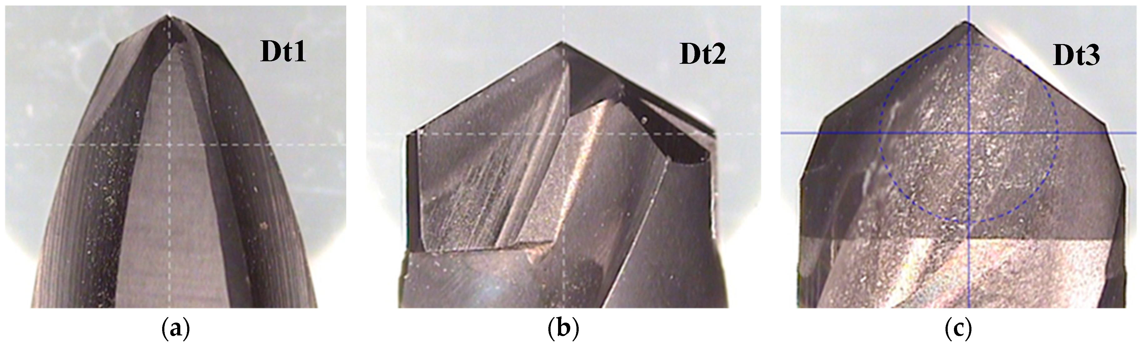
Figure 2.
Holes with lowest and highest surface roughness at the entrance of each drill bit: (a) Low Sa_i, Test 1—Dt1; (b) Low Sa_i, Test 18—Dt2; (c) Low Sa_i, Test 26—Dt3; (d) High Sa_i, Test 3—Dt1; (e) High Sa_i, Test 14—Dt2; (f) High Sa_i, Test 22—Dt3.
Figure 2.
Holes with lowest and highest surface roughness at the entrance of each drill bit: (a) Low Sa_i, Test 1—Dt1; (b) Low Sa_i, Test 18—Dt2; (c) Low Sa_i, Test 26—Dt3; (d) High Sa_i, Test 3—Dt1; (e) High Sa_i, Test 14—Dt2; (f) High Sa_i, Test 22—Dt3.
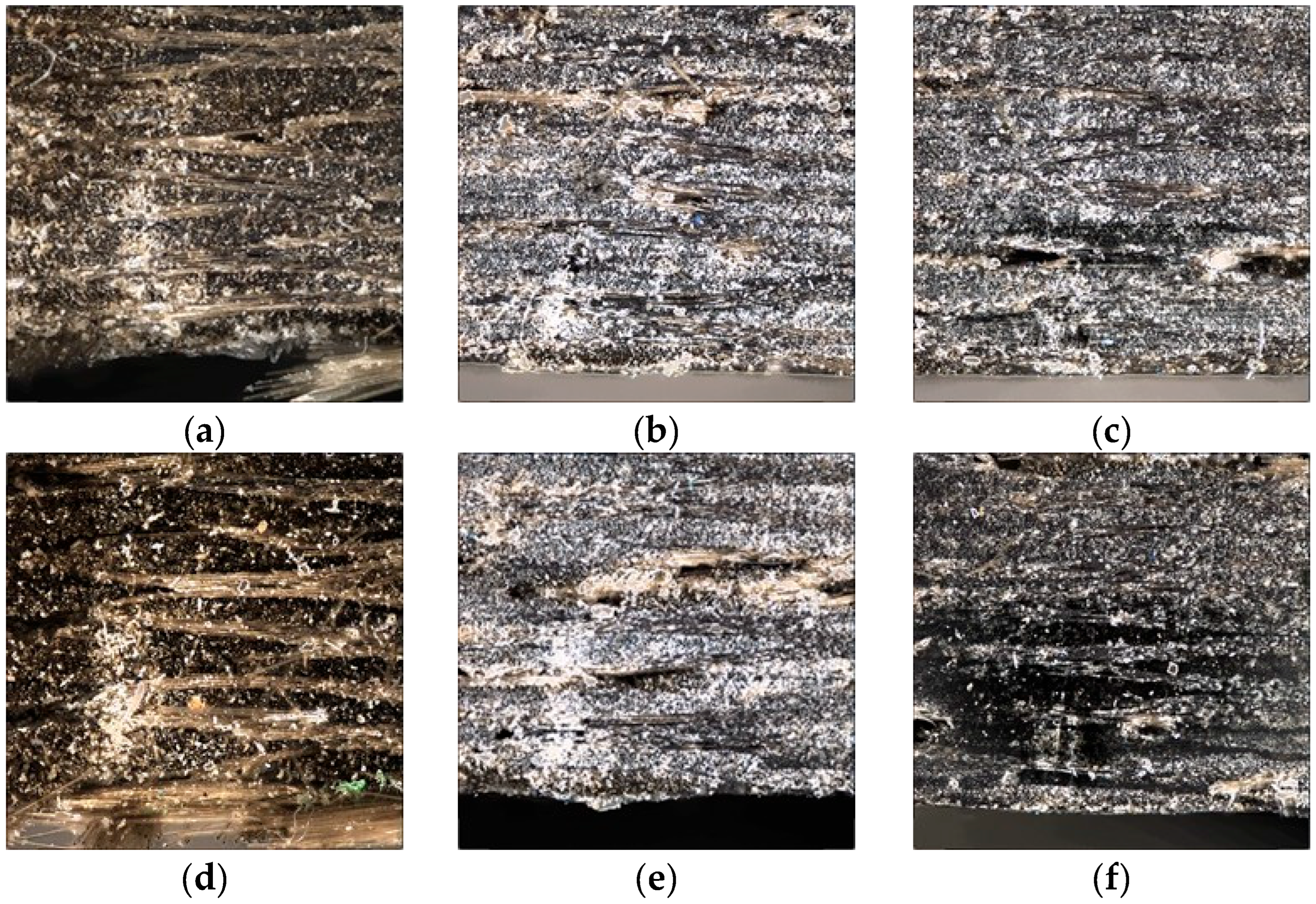
Figure 3.
Holes with lowest and highest surface roughness at the exit of each drill bit: (a) Low Sa_o, Test 9—Dt1; (b) Low Sa_o, Test 11—Dt2; (c) Low Sa_o, Test 19—Dt3; (d) High Sa_o, Test 7—Dt1; (e) High Sa_o, Test 13—Dt2; (f) High Sa_o, Test 25—Dt3.
Figure 3.
Holes with lowest and highest surface roughness at the exit of each drill bit: (a) Low Sa_o, Test 9—Dt1; (b) Low Sa_o, Test 11—Dt2; (c) Low Sa_o, Test 19—Dt3; (d) High Sa_o, Test 7—Dt1; (e) High Sa_o, Test 13—Dt2; (f) High Sa_o, Test 25—Dt3.
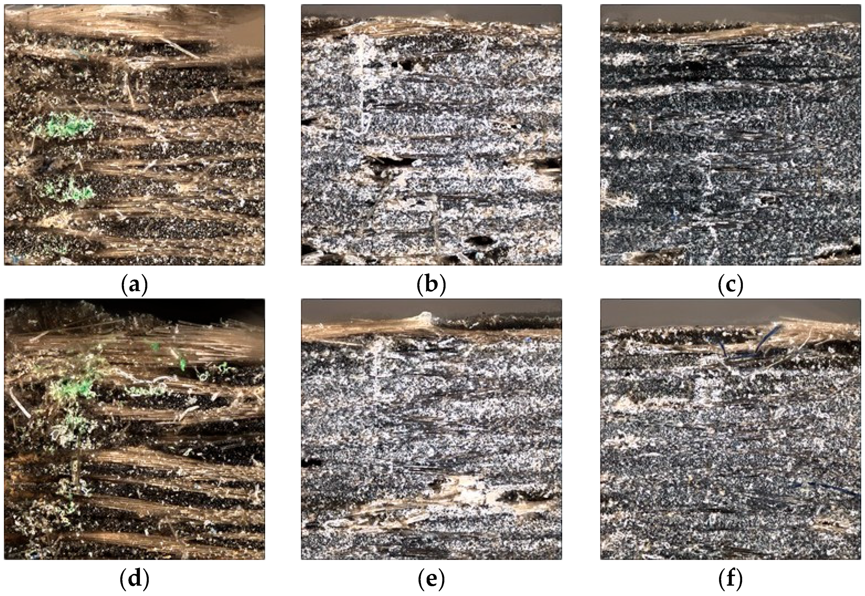
Figure 4.
Estimated response surface of profile roughness: (a) Ra for Dt1; (b) Rz for Dt1; (c) Ra for Dt2; (d) Rz for Dt2; (e) Ra for Dt3; (f) Rz for Dt3.
Figure 4.
Estimated response surface of profile roughness: (a) Ra for Dt1; (b) Rz for Dt1; (c) Ra for Dt2; (d) Rz for Dt2; (e) Ra for Dt3; (f) Rz for Dt3.
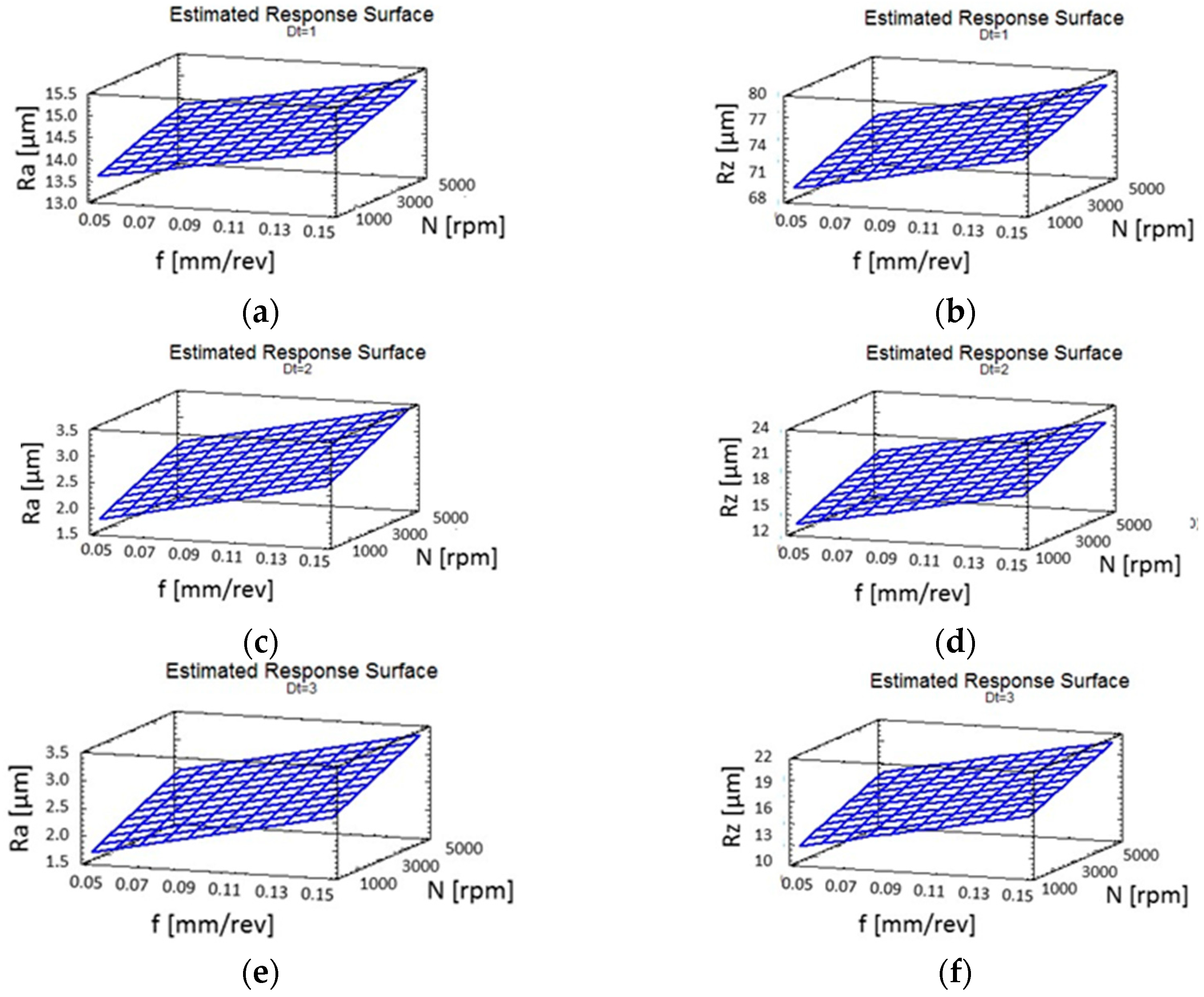
Figure 5.
Estimates response surface of surface roughness: (a) Sa_i for Dt1; (b) Sa_o for Dt1; (c) Sa_i for Dt2; (d) Sa_o for Dt2; (e) Sa_i for Dt3; (f) Sa_o for Dt3; (g) Sz_i for Dt1; (h) Sz_o for Dt1; (i) Sz_i for Dt2; (j) Sz_o for Dt2; (k) Sz_i for Dt3; (l) Sz_o for Dt3.
Figure 5.
Estimates response surface of surface roughness: (a) Sa_i for Dt1; (b) Sa_o for Dt1; (c) Sa_i for Dt2; (d) Sa_o for Dt2; (e) Sa_i for Dt3; (f) Sa_o for Dt3; (g) Sz_i for Dt1; (h) Sz_o for Dt1; (i) Sz_i for Dt2; (j) Sz_o for Dt2; (k) Sz_i for Dt3; (l) Sz_o for Dt3.
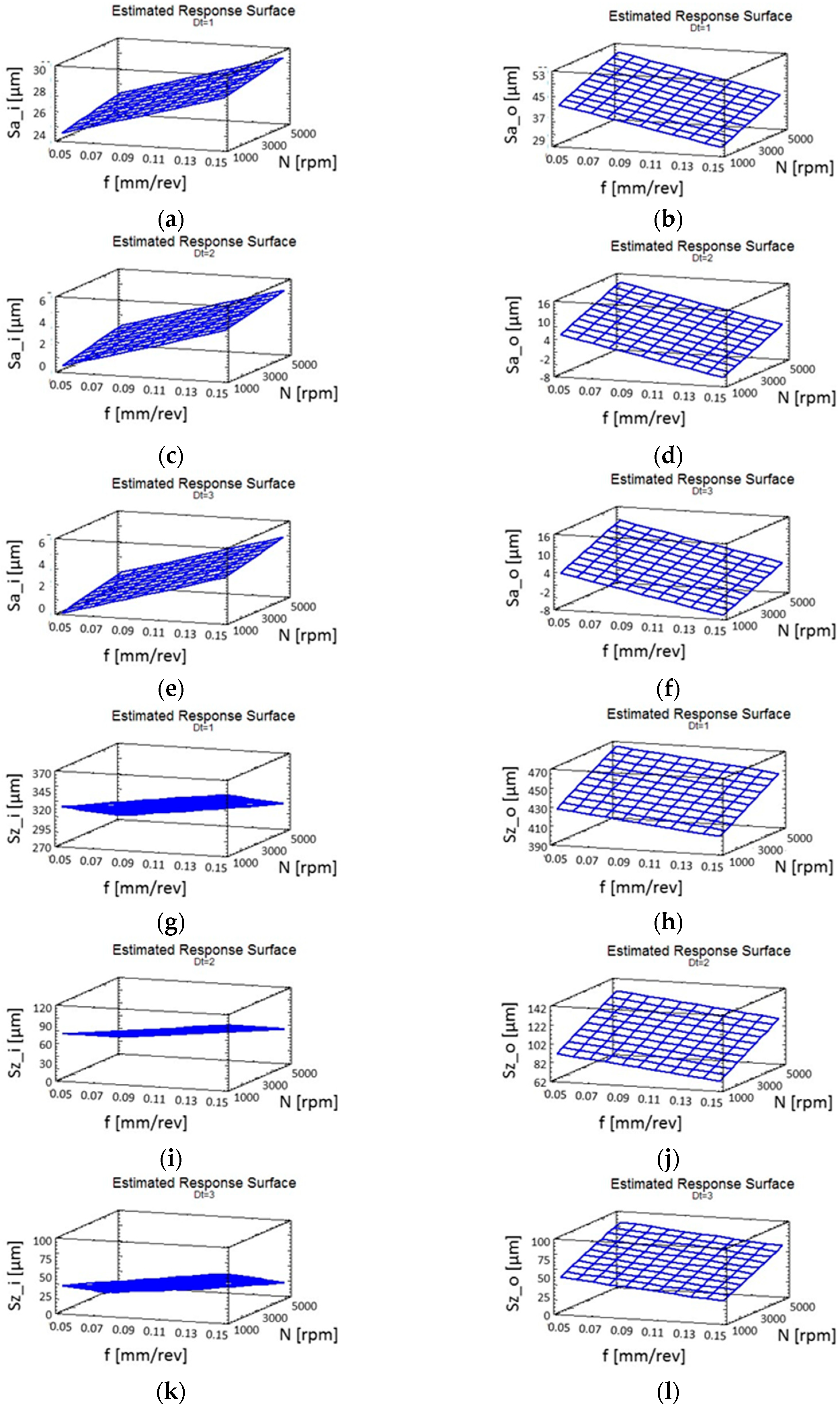
Figure 6.
Workflow followed to train the ML algorithms.
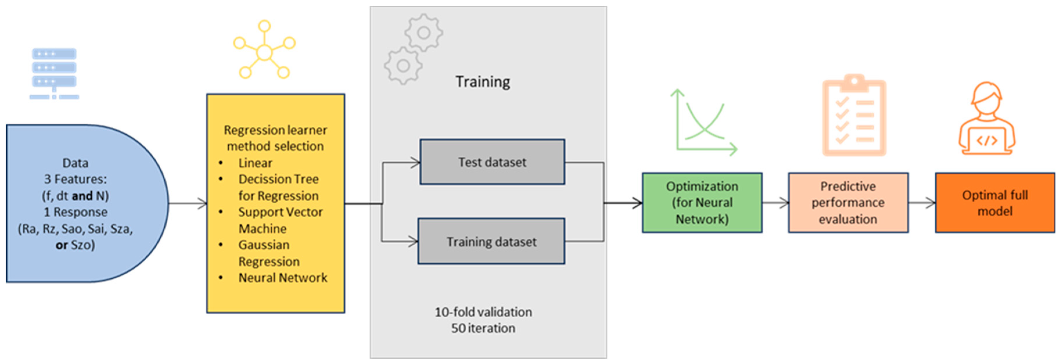
Figure 7.
Correlation matrix plot for the responses.
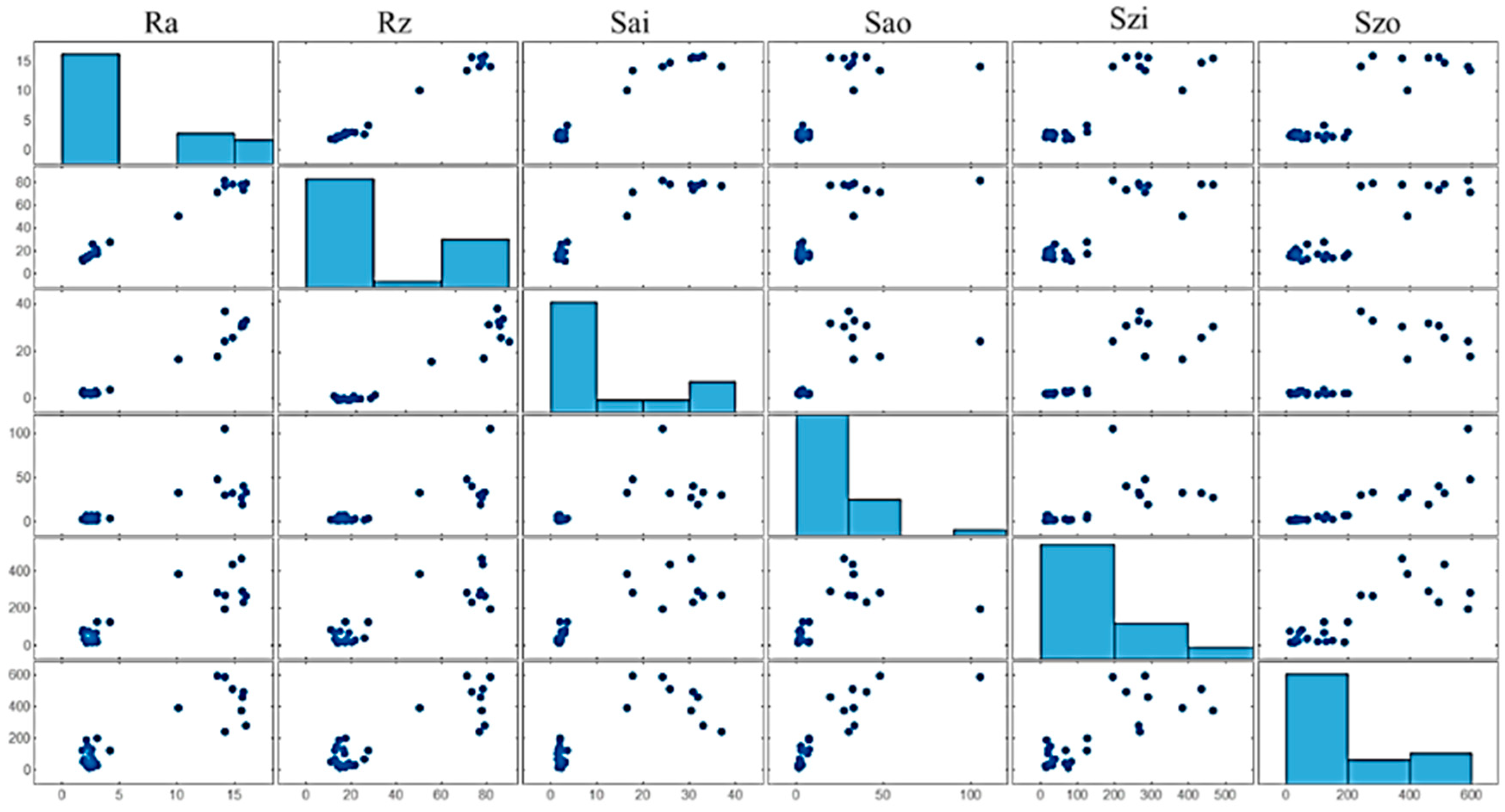
Figure 8.
Features plot with error bar for the more accurate model trained for Ra and Rz (left). Features plot with error bar for the second more accurate model trained for Ra and Rz (right).
Figure 8.
Features plot with error bar for the more accurate model trained for Ra and Rz (left). Features plot with error bar for the second more accurate model trained for Ra and Rz (right).
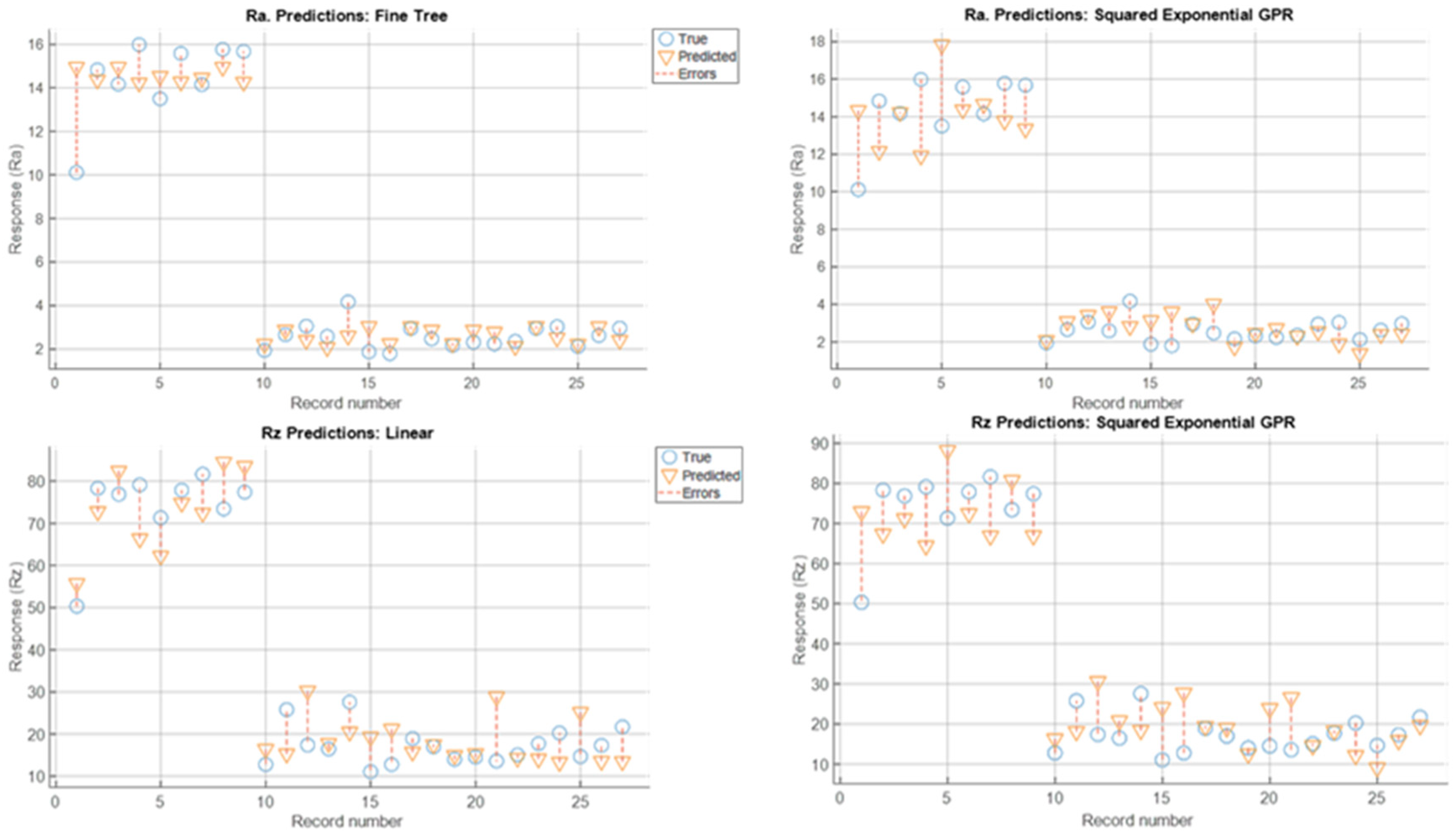
Figure 9.
Features plot with error bar for the more accurate model trained for Sa_i and Sa_o (left). Features plot with error bar for the second more accurate model trained for Sa_i and Sa_o (right).
Figure 9.
Features plot with error bar for the more accurate model trained for Sa_i and Sa_o (left). Features plot with error bar for the second more accurate model trained for Sa_i and Sa_o (right).
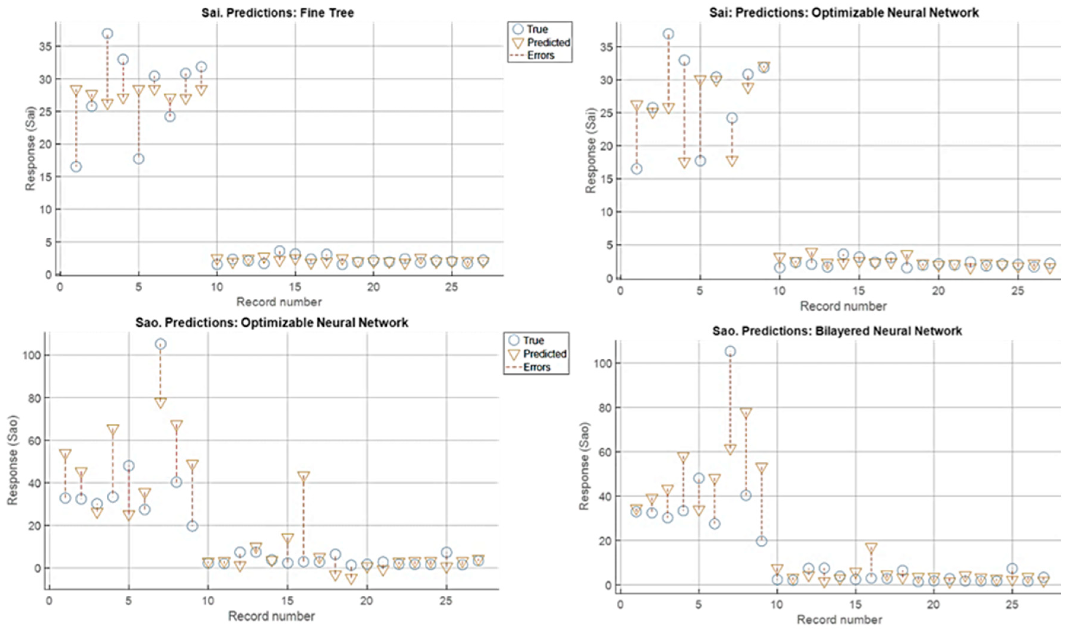
Figure 10.
Features plot with error bar for the more accurate model trained for Sz_i and Sz_o (left). Features plot with error bar for the second more accurate model trained for Sz_i and Sz_o (right).
Figure 10.
Features plot with error bar for the more accurate model trained for Sz_i and Sz_o (left). Features plot with error bar for the second more accurate model trained for Sz_i and Sz_o (right).
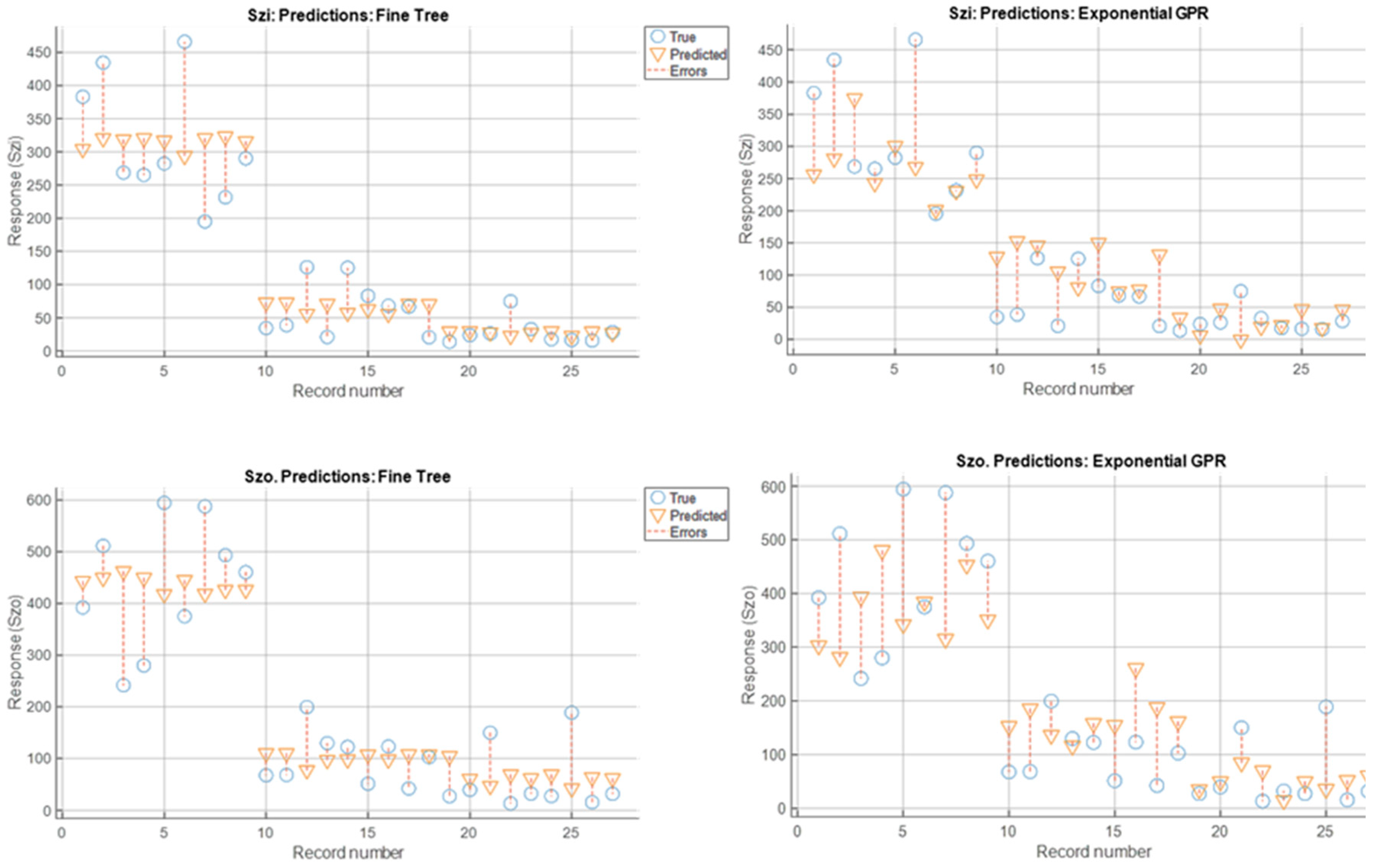

Table 1.
Main characteristics of drill bits.
| Drill bit type | Dt1 | Dt2 | Dt3 |
|---|---|---|---|
| Material | Solid carbide | Solid carbide | Solid carbide |
| Coating type | Polycrystalline diamond (point angle) | Polycrystalline diamond (point angle) | Polycrystalline diamond sintering (point angle and surface cutting surface) |
| Cutting edge length [mm] | 50 | 57 | 28 |
| Cutting edges | 3 | 2 | 2 |
| Cutting edges type | Straight flutes | Helical flutes | Helical flutes |
| Point angle [°] | 83 | 120 | 120 |
| Helix angle [°] | 0 | 30 | 30 |
| Drill bit tolerance | H7 | m7 | h7 |
Table 2.
Experimental data.
| Test number | N [rpm] | f [mm/rev] | Dt [code] | Ra [μm] | Rz [μm] | Sa_i [μm] | Sz_i [μm] | Sa_o [μm] | Sz_o [μm] |
|---|---|---|---|---|---|---|---|---|---|
| 1 | 1000 | 0.05 | 1 | 10.119 | 50.345 | 16.511 | 383.096 | 32.896 | 392.203 |
| 2 | 1000 | 0.10 | 1 | 14.834 | 78.298 | 25.772 | 434.508 | 32.416 | 511.331 |
| 3 | 1000 | 0.15 | 1 | 14.173 | 76.863 | 36.946 | 268.618 | 30.193 | 241.758 |
| 4 | 3000 | 0.05 | 1 | 15.986 | 79.125 | 32.974 | 265.204 | 33.351 | 280.127 |
| 5 | 3000 | 0.10 | 1 | 13.505 | 71.316 | 17.726 | 282.398 | 48.042 | 594.483 |
| 6 | 3000 | 0.15 | 1 | 15.583 | 77.870 | 30.403 | 465.946 | 27.481 | 374.971 |
| 7 | 5000 | 0.05 | 1 | 14.151 | 81.637 | 24.208 | 195.184 | 105.269 | 587.836 |
| 8 | 5000 | 0.10 | 1 | 15.773 | 73.420 | 30.820 | 231.519 | 40.340 | 493.150 |
| 9 | 5000 | 0.15 | 1 | 15.678 | 77.405 | 31.837 | 290.223 | 19.649 | 460.289 |
| 10 | 1000 | 0.05 | 2 | 1.945 | 12.781 | 1.521 | 34.446 | 2.317 | 67.552 |
| 11 | 1000 | 0.10 | 2 | 2.664 | 25.801 | 2.322 | 38.586 | 2.064 | 68.329 |
| 12 | 1000 | 0.15 | 2 | 3.056 | 17.387 | 2.065 | 126.174 | 7.397 | 199.549 |
| 13 | 3000 | 0.05 | 2 | 2.588 | 16.474 | 1.653 | 21.031 | 7.478 | 129.861 |
| 14 | 3000 | 0.10 | 2 | 4.172 | 27.587 | 3.574 | 125.344 | 3.818 | 122.585 |
| 15 | 3000 | 0.15 | 2 | 1.879 | 11.051 | 3.122 | 83.015 | 2.366 | 51.312 |
| 16 | 5000 | 0.05 | 2 | 1.797 | 12.778 | 2.357 | 68.052 | 2.947 | 123.341 |
| 17 | 5000 | 0.10 | 2 | 2.952 | 18.933 | 3.058 | 66.530 | 2.859 | 42.324 |
| 18 | 5000 | 0.15 | 2 | 2.471 | 16.984 | 1.512 | 20.634 | 6.427 | 102.831 |
| 19 | 1000 | 0.05 | 3 | 2.168 | 14.004 | 1.890 | 13.679 | 1.314 | 27.198 |
| 20 | 1000 | 0.10 | 3 | 2.320 | 14.526 | 2.132 | 23.675 | 1.737 | 39.597 |
| 21 | 1000 | 0.15 | 3 | 2.243 | 13.589 | 1.934 | 26.260 | 2.799 | 150.085 |
| 22 | 3000 | 0.05 | 3 | 2.362 | 15.065 | 2.403 | 74.714 | 1.718 | 13.267 |
| 23 | 3000 | 0.10 | 3 | 2.954 | 17.742 | 1.786 | 32.852 | 1.706 | 32.349 |
| 24 | 3000 | 0.15 | 3 | 3.034 | 20.252 | 2.080 | 17.473 | 1.662 | 27.372 |
| 25 | 5000 | 0.05 | 3 | 2.128 | 14.668 | 2.026 | 16.466 | 7.337 | 188.813 |
| 26 | 5000 | 0.10 | 3 | 2.630 | 17.297 | 1.664 | 15.671 | 1.528 | 15.616 |
| 27 | 5000 | 0.15 | 3 | 2.972 | 21.696 | 2.177 | 28.278 | 3.369 | 31.781 |
Table 3.
ANOVA results for measured outputs.
| Model | Dt | f | N | Residual | ||
|---|---|---|---|---|---|---|
| Ra | P-value | 0.0000 | 0.0000 | 0.1043 | 0.1431 | − |
| Contribution | 97.00% | 96.30% | 0.39% | 0.31% | 2.99% | |
| Rz | P-value | 0.0000 | 0.0000 | 0.1967 | 0.2635 | − |
| Contribution | 95.58% | 94.96% | 0.36% | 0.26% | 4.42% | |
| Sa_i | P-value | 0.0000 | 0.0000 | 0.1308 | 0.6174 | − |
| Contribution | 91.74% | 90.72% | 0.92% | 0.096% | 8.26% | |
| Sa_o | P-value | 0.0000 | 0.0000 | 0.1340 | 0.2148 | − |
| Contribution | 68.02% | 62.12% | 3.52% | 2.37% | 31.98% | |
| Sz_i | P-value | 0.0000 | 0.0000 | 0.3057 | 0.1005 | − |
| Contribution | 86.08% | 83.53% | 0.69% | 1.86% | 13.92% | |
| Sz_o | P-value | 0.0000 | 0.0000 | 0.6521 | 0.3598 | − |
| Contribution | 82.22% | 81.34% | 0.17% | 0.71% | 17.78% |
Table 4.
Parameter estimated for independent variables.
| Dependent Variable | Parameters | RSquare | RSquare adj. | ||||
|---|---|---|---|---|---|---|---|
| I1 | I2 | f | N | Intercept | |||
| Ra | 7.9 | 3.91 | 8.72 | 0.0002 | 5.07 | 97.01% | 96.46% |
| Rz | 37.92 | 18.35 | 40.24 | 0.00087 | 29.48 | 95.58% | 94.77% |
| Sa_i | 16.86 | 8.26 | 29.48 | 0.00024 | 6.95 | 91.74% | 90.24% |
| Sa_o | 25.13 | 11.76 | 103.65 | 0.0021 | 19.93 | 68.02% | 62.20% |
| Sz_i | 177.8 | 70.3 | 283.05 | 0.012 | 141.57 | 86.09% | 83.55% |
| Sz_o | 238.46 | 98.03 | 189.17 | 0.0097 | 188.77 | 82.22% | 79.00% |
* I1 = 1 if Dt = 1, −1 if Dt = 3, 0 otherwise; I2= 1 if Dt = 2, −1 if Dt = 3, 0 otherwise.
Table 5.
Regression learner algorithms trained using the experimental data.
| Regression learner | Type | Description |
|---|---|---|
| LR | Linear | Classic linear regression |
| LRi | Linear interaction regression (considering intercept, linear and interaction terms) that applies the interaction between predictions | |
| LRsw | Stepwise linear regression | |
| TF | Decision Tree for Regression | Fine Tree. Minimum leaf size=4 |
| TM | Medium Tree. Minimum leaf size=12 | |
| SVMc | Support Vector Machine | Support Vector Machine configured with Cubic kernel |
| GPRs | Gaussian Regression | Gaussian process regression configured with a Square Exponential Kernel Function |
| GPRr | Gaussian process regression configured with a Rational Kernel Function | |
| GPRm | Gaussian process regression configured with a Mattern 5/2 Kernel Function | |
| NNOpt | Neural Network | Neural Network optimized with the following hyperparameters: |
| Connected Layers: 3 | ||
| First layer sixe: 10 | ||
| Second sixe: 10 | ||
| Third layer sixe: 10 | ||
| Activation function: Rectified Linear Unit (ReLU) | ||
| Iteration limit | ||
| Regularization Strenght (Lambda): 0 | ||
| Standarize data: on |
Table 6.
Features used to train the prediction models and responses obtained for each one of the models. Each model is trained to give a unique response using the three features.
Table 6.
Features used to train the prediction models and responses obtained for each one of the models. Each model is trained to give a unique response using the three features.
| Parameter | Symbol | Feature/Response |
|---|---|---|
| Rotation speed | N | Feature (numerical) |
| Feed rates | f | Feature (numerical) |
| Tool | Dt | Feature (categorical codified) |
| Average roughness | Ra | Response |
| Maximum height of profile | Rz | Response |
| Arithmetic mean height (input of the drill bit) | Sa_i | Response |
| Arithmetic mean height (output of the drill bit) | Sa_o | Response |
| Maximum height (input of the drill bit) | Sz_i | Response |
| Maximum height (output of the drill bit) | Sz_o | Response |
Table 7.
Quantitative predictive performance results for the trained models.
| Response | Learning method | RMSE | MAE | RSquare* |
|---|---|---|---|---|
| Ra | TF | 1.237 | 0.768 | 0.96 |
| GPRr | 1.830 | 1.308 | 0.90 | |
| Rz | LRsw | 5.244 | 4.429 | 0.97 |
| GPRr | 9.817 | 7.905 | 0.88 | |
| Sa_i | TF | 4.103 | 2.3351 | 0.90 |
| NNOpt | 4.969 | 2.615 | 0.86 | |
| Sa_o | NNOpt | 15.657 | 10.504 | 0.57 |
| TF | 15.910 | 7.460 | 0.53 | |
| Sz_i | TF | 58.727 | 42.320 | 0.85 |
| GPRs | 74.360 | 51.861 | 0.75 | |
| Sz_o | TF | 94.107 | 71.993 | 0.76 |
| TF | 120.05 | 93.109 | 0.63 |
* Correlation: predicted VS real value.
Disclaimer/Publisher’s Note: The statements, opinions and data contained in all publications are solely those of the individual author(s) and contributor(s) and not of MDPI and/or the editor(s). MDPI and/or the editor(s) disclaim responsibility for any injury to people or property resulting from any ideas, methods, instructions or products referred to in the content. |
© 2026 by the authors. Licensee MDPI, Basel, Switzerland. This article is an open access article distributed under the terms and conditions of the Creative Commons Attribution (CC BY) license (http://creativecommons.org/licenses/by/4.0/).
Copyright: This open access article is published under a Creative Commons CC BY 4.0 license, which permit the free download, distribution, and reuse, provided that the author and preprint are cited in any reuse.


